Article

Monitoring and Modelling Coastal Vulnerability and Mitigation Proposal for an Archaeological Site (Kaulonia, Southern Italy)

by
Diana Di Luccio
1,*,
Guido Benassai
2,*,
Gianluigi Di Paola
3,
Carmen Maria Rosskopf
3,
Luigi Mucerino
4,
Raffaele Montella
1 and
Pasquale Contestabile
5
1
Department of Science and Technologies, University of Naples “Parthenope”, 80133 Napoli, Italy
2
Department of Engineering, University of Naples “Parthenope”, 80133 Napoli, Italy
3
Department of Biosciences and Territory, University of Molise, 86090 Pesche, Italy
4
Department of Earth, Environment and Life Sciences, University of Genova, 16126 Genova, Italy
5
Department of Engineering, University of Campania “Luigi Vanvitelli”, 81031 Aversa (Caserta), Italy
*
Authors to whom correspondence should be addressed.
Sustainability 2018, 10(6), 2017; https://0-doi-org.brum.beds.ac.uk/10.3390/su10062017
Submission received: 19 May 2018 / Revised: 5 June 2018 / Accepted: 7 June 2018 / Published: 14 June 2018

Abstract

:
This paper presents a Coastal Vulnerability Assessment (CVA) of a microtidal beach located on the Ionian Sea in Calabria region (southern Italy) in order to examine the influence of the different run-up equations on CVA score and propose mitigation measures for the most vulnerable parts of the beach. The coastal area has been severely eroded by extreme wave storms, which have also damaged important archaeological structures located on a nearby cliff. A typical 1 year return period (Tr) storm, associated with the recent criticalities, was chosen to test the different run-up formulas (Holman (1986), Mase (1989) Stockdon et al. (2006) and Poate et al. (2016)) on a number of beach profiles in order to check the sensitivity of the CVA calculation with regard to the different run-up equations. The obtained results provide evidence that different run-up levels often give rise to different CVA scores. Based on vulnerability results, some mitigation measures have been proposed for the beach in front of the archaeological area, based on submerged detached breakwater and an adherent gabion wall for the cliff defence.

1. Introduction

The complex multi-dimensional behaviour of coastal systems to a wide range of stresses and perturbations requires a strategic approach for the management of the coastal environment. Continual flooding, coastal erosion and loss of livelihood of coastal communities appear in fact to be increasing in intensity given accelerated global climate change [1].
The Coastal Vulnerability Index (CVI), introduced by Gornitz [1], was based on seven physical variables, associated with inundation and erosion hazard related in a quantitative manner. This index, suitable for regional studies, was used by a number of researcher both in Mediterranean context, as De Leo et al. [2] and Besio et al. [3] and in ocean coastal sites as in Di Paola et al. [4]. Moreover, with the addition of demographic variables, the CVI was transformed in the Social Vulnerability Index (SVI) [5,6].
A more specific coastal hazard index, which needs local information in the Coastal Vulnerability Assessment (CVA) [4], was used in this paper. We applied this index for examining strategies that can reduce the vulnerability, particularly in severely damaged coastal areas. The mechanism of wave attack on the beach is schematized with two contributions, the first linked with coastal inundation (and relative wave run-up evaluation) and the second associated with the short-term beach erosion. These contributions have already been used to evaluate the coastal vulnerability and risk [7], due to wave storms, sea level rise [8] and subsidence [9].
In CVA, the wave run-up, defined as the time-varying location of the shoreward edge of water on the beach face, is statistically processed, associated with its maximum length Xmax, and normalized through the beach width L to give a beach inundation index IRu. The sensitivity of the CVA index with respect to the different run-up equations on several profiles of a micro-tidal beach located on the Ionian Sea in the Calabria region (southern Italy), was examined. Moreover, based on vulnerability results, a mitigation strategy for the archaeological area above a nearby cliff, subjected to severe wave attack during several storm events occurring in 2013 and 2014, was conceived calculating the lowering of the CVA with a proper index recently introduced [10].
In the following, we examine the main equations for run-up evaluation, which is a major parameter for assessing coastal vulnerability. In most equations, the run-up is statistically parametrized in terms of exeedance percentage Ru2% normalized by H0 deep water significant wave height, and linked with Iribarren number [11]
ξ 0 = tan β H 0 L 0 ,
where β is the beach slope and L0 is the deep water wave length. Low Iribarren numbers ( ξ 0 < 1) indicate dissipative and intermediate conditions, while higher values ( ξ 0 > 1) indicate reflective conditions.
Holman [12] proposed an empirical formula to obtain Ru2%, based on Iribarren number ξ f constrained with the foreshore slope β f.
R u 2 % H 0 = 0.83 ξ f + 0.2 ,
in which the first term is related to the infra-gravity component while the second one is linked to the swell component.
Similarly, Stockdon et al. [13] expressed Ru2% as a function of wave setup and swash, as given in Equation (3):
R u 2 % = 1.1 0.35 tan β f H 0 L 0 0.5 + H 0 L 0 0.563 tan β f 2 + 0.004 0.5 2 ,
where β f is the foreshore slope.
Another empirical formula was proposed by Mase [14] who obtained the run-up level Ru2% as a function of the empirical coefficients a and b, set as a = 1.89 and b = 0.71:
R u x % H 0 = a ξ b .
More recently, Poate et al. [15] introduced a new simplified formula that depends on both local significant wave height Hs, the total beach slope β and mean wave period Tm
R u 2 % = C tan β 0.5 T m H s ,
where C is a constant fixed to 0.49 by Poate et al. [15].
In order to investigate the CVA sensitivity to these wave run-up formulas, Equations (2)–(5) are examined and discussed with regard to their influence on the whole CVA calculation. Then, a mitigation strategy that could reduce the high vulnerability in the area occupied by the archaeological site was proposed, taking into account the structure typology and position.
The analysis started with the wave simulations based on the WaveWatch III (WWIII) wave model, implemented by Campania Center for Marine and Atmospheric Monitoring and Modelling (CCMMMA)—University of Naples “Parthenope” [16]. This model, in use in southern Italy since 2006 [17,18,19], was first verified in offshore conditions by in situ measurements provided by the Italian Sea Wave Measurement Network buoy of Crotone [20] and then implemented for the tested micro-tidal beach. The run-up levels associated with a typical one-year return period storm were used in the standard CVA evaluation, as conceived by Di Paola et al. [21] and Benassai et al. [22]. To this aim, the offshore wave simulations were first validated with field measurements [23,24] and then used as initial conditions for run-up calculations.
The paper is organized as follows: the study area is presented in Section 2, the methodology is reported in Section 3, results are given in Section 4, and the adaptation strategy is reported in Section 5. Finally, the discussion and conclusions are given in Section 6 and Section 7, respectively.

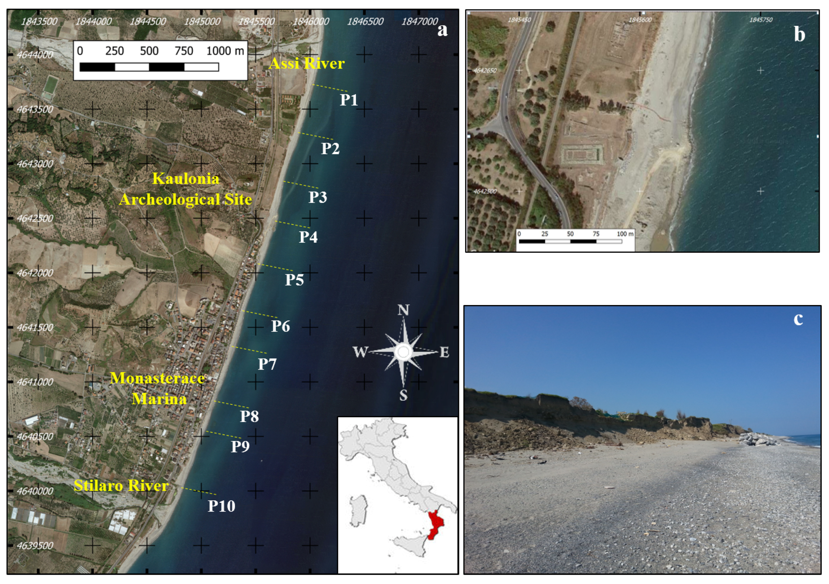
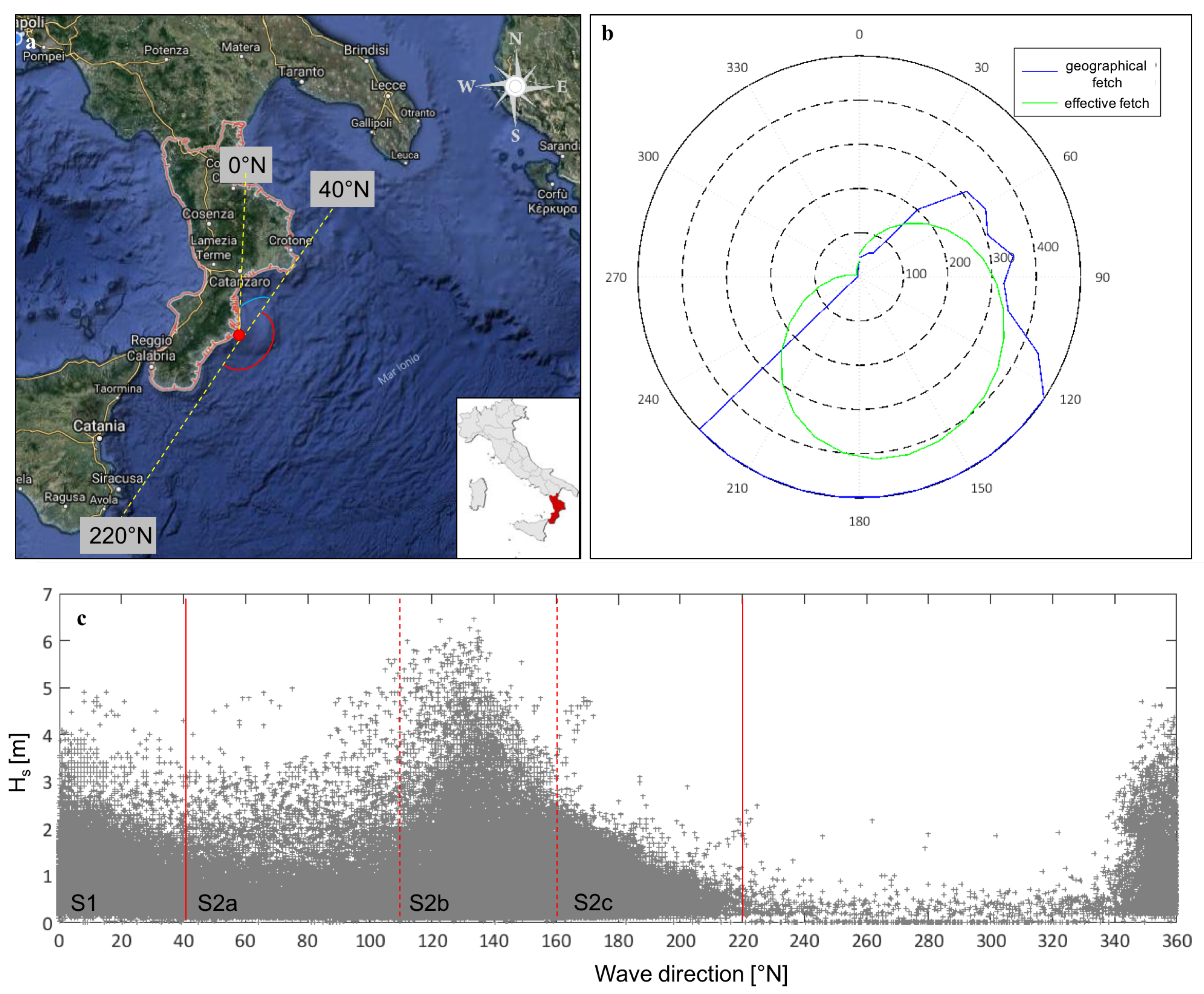
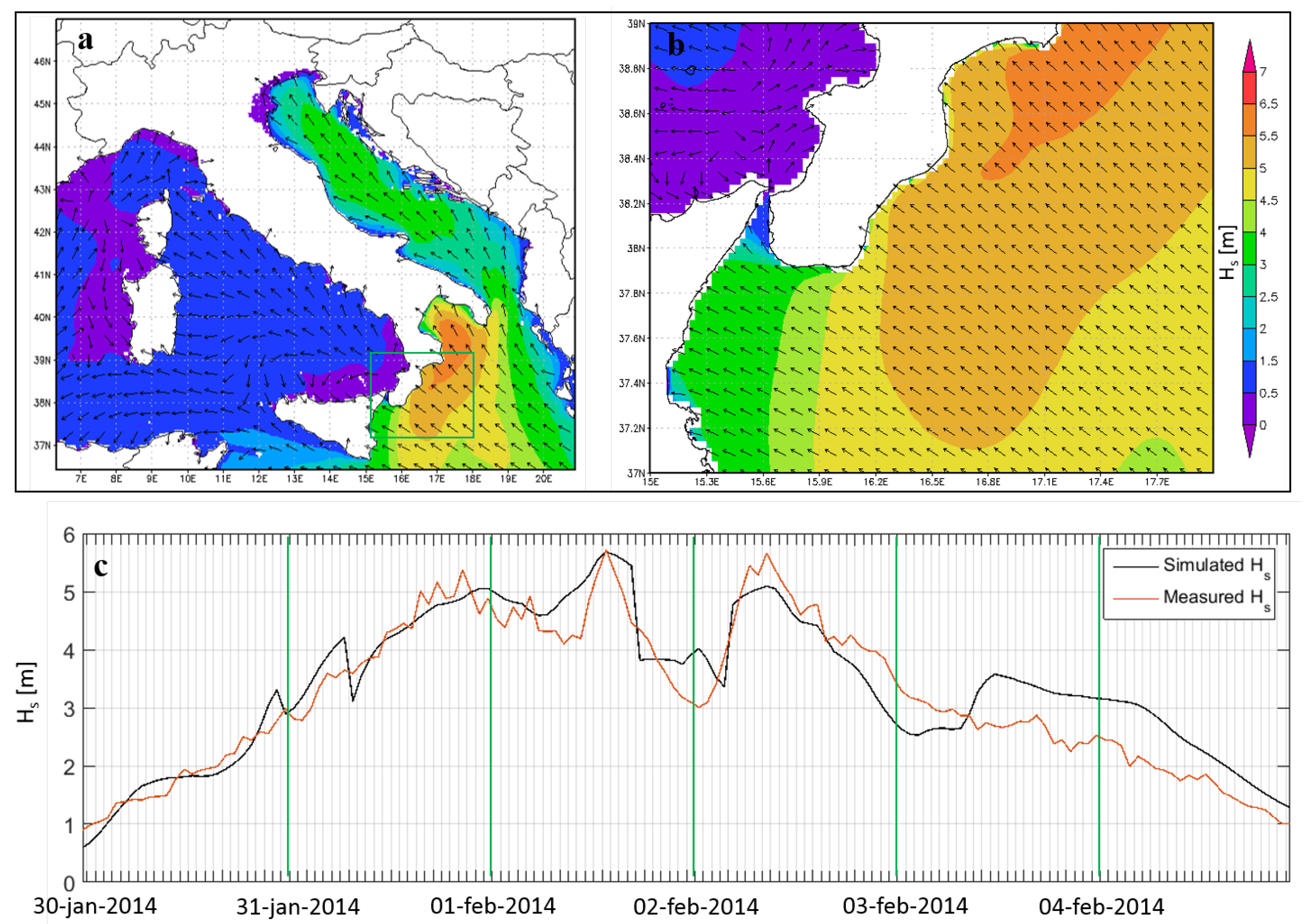
2. Study Area and Wave Climate

The study area coincides with a ca. 3.5 km long beach stretch, located along the southern Ionian coast of Calabria in the municipality of Monasterace Marina (province of Reggio Calabria, Italy), bordered by the Assi and Stilaro torrents (Figure 1a).
This coastal area is part of the sector Punta Stilo—Capo Spartivento [25], which forms a slightly curved, low-gradient, wave-dominated coast associated with micro-tidal ranges. The sandy to mixed sand-gravel beaches are fed by numerous so-called Calabrian fiumare such as the Assi and Stilaro torrents, i.e., ephemeral streams with typical braided riverbeds that drain steep and rather short hilly slopes, with a hydrological regime closely dependent on rainfall distribution [26].
The longitudinal sediment transport is very variable and constrained by the prevailing winds. In more detail, drift is from north to south during the storms coming from the east and southeast, while it changes direction when storms come from the south. However, the prevailing drift is from north to south, with a quantity of mobilized material equal to 70.000 m3/yr [27].
The well-known archaeological area of Kaulonia, a Magna Graecia colony founded in the 8th century BC and inhabited up until the 2nd century BC, lies just landward of the beach. The remnants of Kaulonia are located on a terraced coastal plain (Figure 1b), overhanging the beach and separated from it by a steep ~5 m high sea-cliff (Figure 1b,c).
The coast is open to waves coming from east and south-east (40° N–220° N), while it is protected from the northeastern waves. The main fetches are found between the directions 40° N and 220° N (in the following S2), while the secondary fetches are found between the directions 0° N and 40° N (in the following S1) (Figure 2a,b).
The offshore wave climate was determined through a statistical analysis of the wave parameters recorded by the Crotone buoy (39°01′06″ N; 17°13′18″ E—Italian Sea Measurement Network—http://dati.isprambiente.it) [20]. Wave data refer to the period January 1990–December 2013 and comprise a total of 115.651 wave records, each characterized by Hs, Tm and Dm. Figure 2c provides the entire data set of pairs of Hs, Dm, divided into secondary fetch S1 and main fetch S2, subsequently subdivided into three sub-sectors: 40–110° N (S2a), 110–160° N (S2b) and 160–220° N (S2c). Each sub-sector is characterized by different wave conditions: Hs lower than 5.5 m for S2a and S2c and Hs higher than 5.5 m for S2b (Figure 2). The historical series of Hs was elaborated to obtain a representative sample of extreme wave events, based on of the Peak Over Threshold method [28], as prescribed by Mathiesen et al. [29]. Table 1 provides the offshore wave heights obtained for each part of the main sector, according to the relative return period Tr, which are maximum for the external directions (sector S2b), with Hs > 5.5 m.
In order to evaluate wave run-up levels associated with frequent wave conditions, a recent storm was selected (February 2014) from eastern directions with significant wave heights occurring at least once a year (i.e., a return period of one year).
For this storm, the numerical wave simulations have been performed using a WWIII model; the wave condition has been a starter point to model run-up calculations using the empirical Formulas (2)–(5).

Archaeological Aspects

The study area, owing to the presence of the Archaeological Park of the Magna Grecia colony of Kaulonia, has a strong historical and cultural identity. The ancient city of Kaulonia was founded ca. 700 years B.C. and frequented until the 2nd century B.C.. Its ruins are located on a soil covered, terraced alluvial plain that is separated from the beach by a cliff, up to 5 m high. Kaulonia became a subject of great interest and systematic archaeological activities starting with the excavation campaigns from 1911 to 1916 and the discovery of the basement of the Doric temple, which represents the major archaeological structure of Kaulonia.
One of the most important subsequent archaeological discoveries dates to the end of the 1960s and consists of a mosaic of remarkable beauty representing the famous Dragon of Kaulonia. Since the 1980s until today, numerous excavations and surveys proceeded successfully [32]. In particular, the very recent excavation campaigns in 2012–2014 added very important archaeological findings. Among them, the largest and most articulated Hellenistic mosaic ever found in southern Italy, and the bronze tablet reporting the longest Achaean inscription ever discovered in Magna Graecia.

3. Methodology

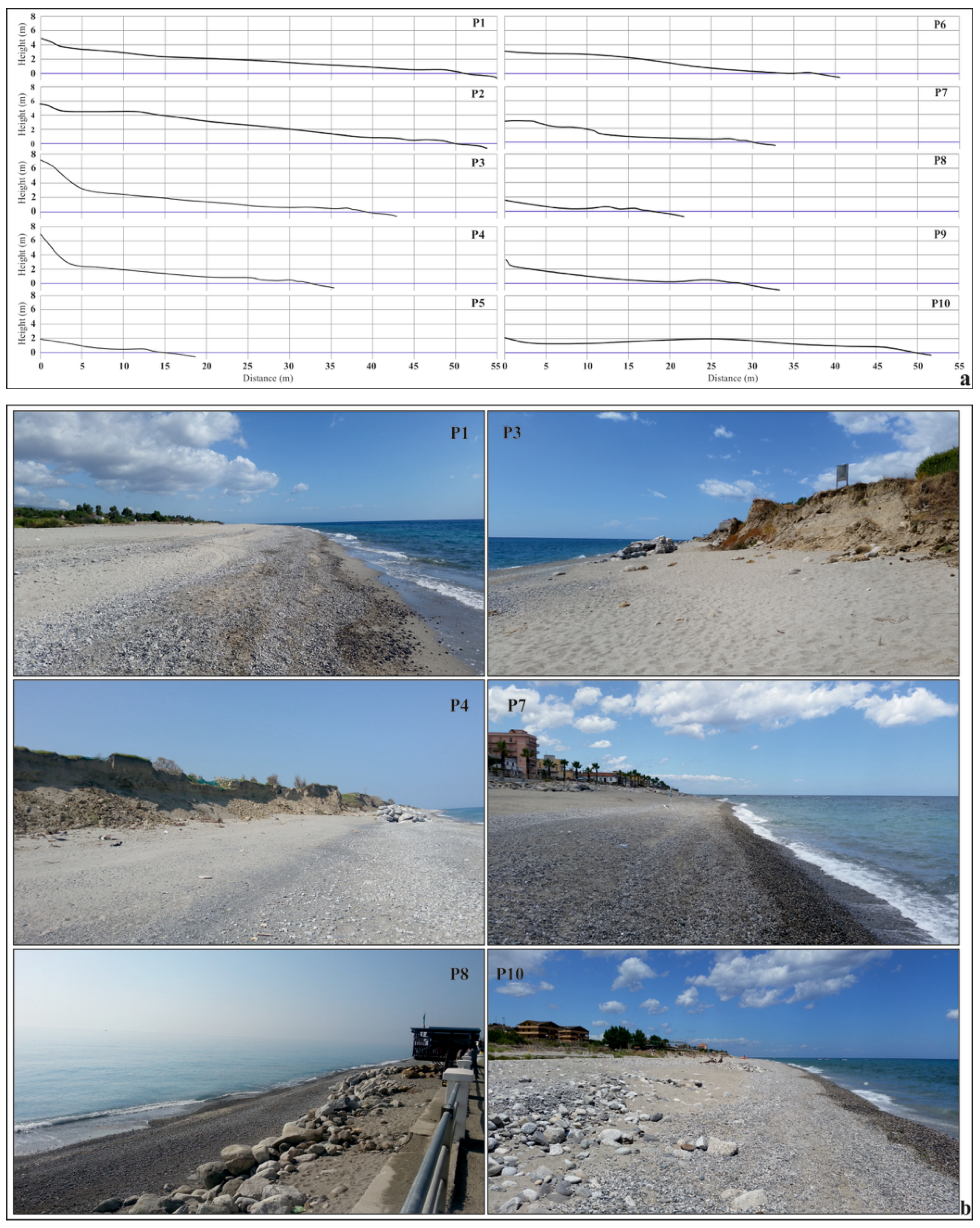
3.1. Topo-Bathymetric and Sediment Survey

In order to characterize the beach morphology, topographic measurements were carried out in July 2014 with a DGPS (Differential Global Positioning Systems) system (Trimble R6), characterized by very high accuracy (Root Mean Square Error − RMSE = ∓0.3 m), which consisted of: (i) shore-normal beach profile surveys, extending from the dune crest/retaining wall down to 1 m water depth, i.e., approximately 4 m distance offshore; and (ii) shoreline delineation. Obtained topographic data refer to 10 beach profiles, from north to south P1–P10 (for location, see Figure 1a and Figure 3a). The shoreline position was calibrated taking into account the micro-tidal excursion determined by ISPRA [33]. A bathymetric survey was performed after the February 2014 wave storm, in order to obtain data also on the submerged beach. A digital single beam gauge coupled with a GPS receiver was used (differential mode DGPS post processing) with an acquisition frequency of 0.5 Hz, obtaining 15 shore-normal transects in calm sea conditions reaching a maximum depth of 12 m.
Grain size analysis was carried out on samples collected in July 2014 by applying the ASTM international standard D421 and D422 [34,35] and the Wentworth scale. The medium to long-term shoreline evolution was investigated considering two periods: 1958–2014 and 1996–2014 in order to provide a view of the overall shoreline evolution since the 1950s as well as of the more recent shoreline changes that have occurred during approximately the last 20 years.

3.2. Numerical Wave Model

The simulation of the offshore wave characteristics has been done with the working scheme [36] implemented by the Campania Center for Marine and Atmospheric Monitoring and Modelling (CCMMMA, [37]) of the University of Naples “Parthenope” [38,39]. The operational configuration is based on the Weather Research and Forecasting (WRF) numerical model [40,41], which gives the atmospheric forcing (10 m wind field) needed to estimate the offshore waves. The wave simulations were carried out using the National Oceanic and Atmospheric Administration (NOAA)/National Centers for Environmental Prediction (NCEP) third-generation wave model WaveWatch III (WWIII) [42,43].
The configured model spatial domain has an extension in latitude from 6.33° N to 20.88° N, and in longitude from 36.42° E to 46.98° E. The model outputs include, among others, gridded fields of significant wave height (Hs), wave direction (Dm), and mean wave period (Tm). The grid points of the WWIII model near the coastline were used as "virtual buoy" (VB) to calculate the wave coastal transformation, with the ultimate goal of simulating the run-up on the beach.

3.3. CVA Method

The coastal vulnerability assessment (CVA) is based on the methodology firstly proposed by Di Paola et al. [4], who calculated this index according to the following equation:
C V A = I R u + I R + I D + E + T ,
where IRu is an index associated with the wave run-up distance, IR is the maximum beach erosion potential index for the shoreline, ID is the backshore coastal protection structures stability index, E is the multi-year beach erosion rate index and T is the tidal range that is negligible in a micro-tidal environment.
The wave run-up height index IRu evaluates the beach potential inundation during wave storms through the run-up distance Xmax, calculated as the horizontal distance that the wave travels during the run-up process, given by the run-up level divided by the foreshore slope ( β f):
X m a x = R u 2 % tan β f .
IRu is obtained from Xmax, normalized to the beach width (L). The index of potential erosion IR provides a measure of the potential retreat of the beach. The IR values depend on the percentage associated with the maximum potential retreat (Rmax) normalized to the width of the beach L. Rmax is evaluated as the maximum value of the general solution associated with the convolution method of Kriebel and Dean [44]:
R ( t ) ) R = 1 2 1 γ 2 1 + γ 2 exp 2 σ t γ 1 1 + γ 2 cos 2 σ t + γ sin 2 σ t ,
R = S W b d b m 0 B + d b S 2 ,
where γ = 2 π T S / T D , i.e., the ratio between the time scale of beach erosion TS and the storm duration TD. In Equations (8) and (9), S is the sea level increase due to wave storm; B is the berm height; β f is the foreshore slope; db is the breaking depth and Wb is the offshore breaking depth distance.
The backshore coastal protection structure index (ID) takes into account the coastal structures, whose efficiency is linked to their transmission coefficient Kt, according to Table 2. Kt was calculated through the following equation [45]:
K t = 0.031 H s D n 50 0.24 R c D n 50 + b ,
where Dn50 is the median nominal diameter of rocks for design conditions, Rc is the freeboard, negative for submerged breakwater. The parameter b is given by:
b = 5.42 s o p + 0.0323 H s D n 50 0.0017 W t D n 50 1.84 + 0.51 ,
where Wt is the width of the top of structure and Sop is the deep-water wave steepness corresponding to peak period Tp:
S o p = 2 π H s g T p 2 .
The ID ranking is reported in Table 2, in which ID assumes negative values, according to Martinelli et al. [10], reducing the overall vulnerability.
Finally, the multi-year beach erosion rate index E, which takes into account the medium-term (20 years) coastline erosion, was derived from the shoreline variations calculated for period 1996–2015.
The resulting CVA index, evaluated according to Equation (6), was divided into four categories, according to the classification defined by Di Paola et al. [4], coming up to the final ranking: very low (CVA = 3), low (3 < CVA ≤ 6), moderate (6 < CVA ≤ 9) and high (9 < CVA ≤ 12) coastal vulnerability (Table 2).

4. Results

4.1. Beach Characterization

The study beach is characterized by a relatively smooth and regular morphology (Figure 3). The landward limit of the backshore is alternatively represented by a few meters high embryonal dune (P1, P2 and P10, Figure 3), an erosion scarp/seacliff increasing in height from north to south up to max 5–6 m (P3–P4, Figure 3), and a seawall of variable height, up to 5 m (P5–P9), limited seawards by boulder barriers in order to improve its resistance to wave-attack (see for instance P7 and P8 in Figure 3). Both the backshore and foreshore zones are composed of mixed-textured, coarse-grained materials. Internal and external areas of the backshore are composed of coarse/very coarse sands and gravels, (see P1 and P3, Figure 3), highlighting a trend to the coarsening of beach sediments from the landward limit of the backshore towards the summer berm. The foreshore is made of sandy gravels with the exception of the areas around the mouths of the Assi and Stilaro streams that are characterized by gravels and gravelly sands, respectively. Median sediment diameters of foreshore sediments (Table 3) range between 2.55 mm and 6.12 mm (P2 and P5 in Table 3). Slope gradients of the backshore β b and foreshore β f range between 2.6–10.5%, and 14.2–20.0%, respectively.
Based on differences in morphology, grain size and anthropic features, the study beach was sub-divided into the following three stretches.
A northern, 0.6 km beach stretch including profiles P1 and P2, which is 25 to 40 m wide and characterized by a low anthropic impact due to the presence of some tourism structures.
A central 0.75 km beach stretch, with an approximate width of 30–35 m. It includes profiles P3, P4 and the archaeological area and is made up of coarse to very coarse sands in the backshore zone, and of sands and gravels in the foreshore zone. Active dunes are completely lacking and the backshore is limited landwards by the erosion scarp/seacliff with the archaeological area. The cliff is made of sandy-gravelly to silty sediments, rich in archaeological material both sparse and organized in several levels. The beach portion in front of the archaeological area was nearly entirely eroded during the storm event on 2 February 2014 and storm waves attacked the cliff directly, causing its local collapse together with some archaeological structures. Because of the extensive damage, a first gabion wall was built in autumn 2014 immediately south to P4 in order to prevent future cliff collapse and avoid further damage to the archaeological site.
Finally, a southern 2 km long beach stretch that extends approximately between P5 and the Stilaro stream mouth (P10) and is characterized by a a high anthropic load mostly due to dense urbanization. The beach, composed of mixed sand and gravel, is 10 to 40 m wide, therefore locally rather narrow (see especially P8, Figure 3 and Table 3). In the past, some coastal defences were realized along this coastal stretch (P7–P8), whose influence has been taken into account through the ID parameter (see Section 4.3.2).

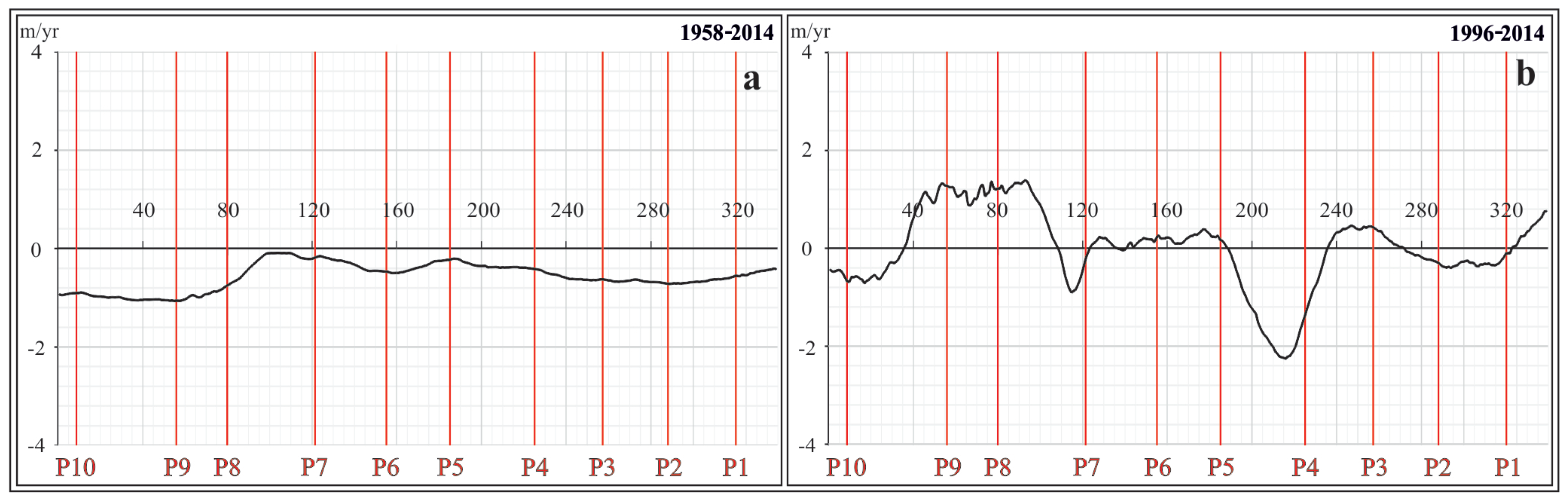
4.2. Medium and Long-Term Shoreline Evolution

In order to evaluate the E parameter in Equation (6), we analyzed the long-term (1958–2014) and the medium-term (1996–2014) shoreline evolution using aerial photographs in scale 1:39.000 (IGMI, 1958), with an accuracy of RMSE = ∓3 m, the regional technical map in scale 1:10.000 (CTR, 1996—RMSE = ∓2 m) and the topographic data provided by DGPS (RMSE = ∓0.3 m) and aerial drone surveys carried out in 2014 (RMSE = ∓1 m). The shoreline position was assumed coincident with the high-water line position that represents the landward limit of wave and water level influences in micro-tidal conditions [46]. Given that the tidal elevation at surveying time was unknown, we assumed an uncertainty between 2 m and 2.8 m for the daily water line position, considering both the minimum (P2) and maximum (P6) beach foreshore slope (Table 3) together with the local daily tidal excursion of about ±20 cm [33]. Moreover, the 2014 shoreline was delineated by interpolating the points obtained with the DGPS surveys with a spatial resolution of 2 m.
Shoreline changes were determined by the overlay of digitized shorelines. Rates of shoreline change were calculated using an extension of ArcGis release 10 (ESRI©), the Digital Shoreline Analysis System (DSAS version 4.0, [47]). This software allowed the creation of 339 transects, spaced 10 m apart, along which the positions of the three shorelines dating to 1958, 1996 and 2014, respectively, were delineated.
With regard to the long-term shoreline evolution, most of the shoreline has experienced a more or less marked erosion (Figure 4a), except for the central portion, around transects P6 and P7 (respectively −6.61 and −5.97 m, Table 4). Severe erosion, instead, occurred within the southern portion (P8–P10, 40 to 60 m retreat) and within the central-northern portion with values up to nearly 40 m in front of the archaeological site of Kaulonia (P3–P4).
In the medium-term (period 1996–2014, Figure 4b and Table 4), the shoreline underwent prevailing progradation (up to 20 m and more, see P8 and P9), whereas some parts of the beach registered again a more or less strong retreat, especially those located in the central-northern part (up to ~33 m, see P4). These results show that the beach in front of the archaeological site has undergone a strong destabilization just over the last 20 years that is still ongoing, as demonstrated by the storm events of 2013 and 2014.
The positive result in terms of shoreline stability of the southern coastal portion, made evident by profiles P6–P9, is most likely related to the realization in 2008 of some coastal protection structures, which have been taken into account in the ID index (see Section 4.3.2).

4.3. CVA Evaluation Based on the February 2014 Storm

The WWIII model was run to simulate the wave conditions during the sea storm of February 2014, validated with Crotone buoy wave measurements. Results are reported in Figure 5a,b (simulations) and Figure 5c (validation). The agreement between the two time series is fairly good; however, non-negligible differences can be noted, as reported in Table 5, which lists the statistical indices introduced by Mentaschi et al. [48] and Melby et al. [49]. It can be noted that the simulated Hs (black line in Figure 5c) is much smoother the one measured by the buoy due to the WWIII incapability to resolve the small scales seen in the buoy records. The correlation coefficient R [48] is 0.933 for Hs, followed by R = 0.826 for Dm and R = 0.672 for Tm, while the Summary Performance Score SPS [49] gives the best agreement for Dm parameter (SPS = 0.914), followed by Hs (SPS = 0.889) and Tm (SPS = 0.771). These results support the reliability of the WWIII simulations, which allow us to use them as a starting point in the run-up model calculation.

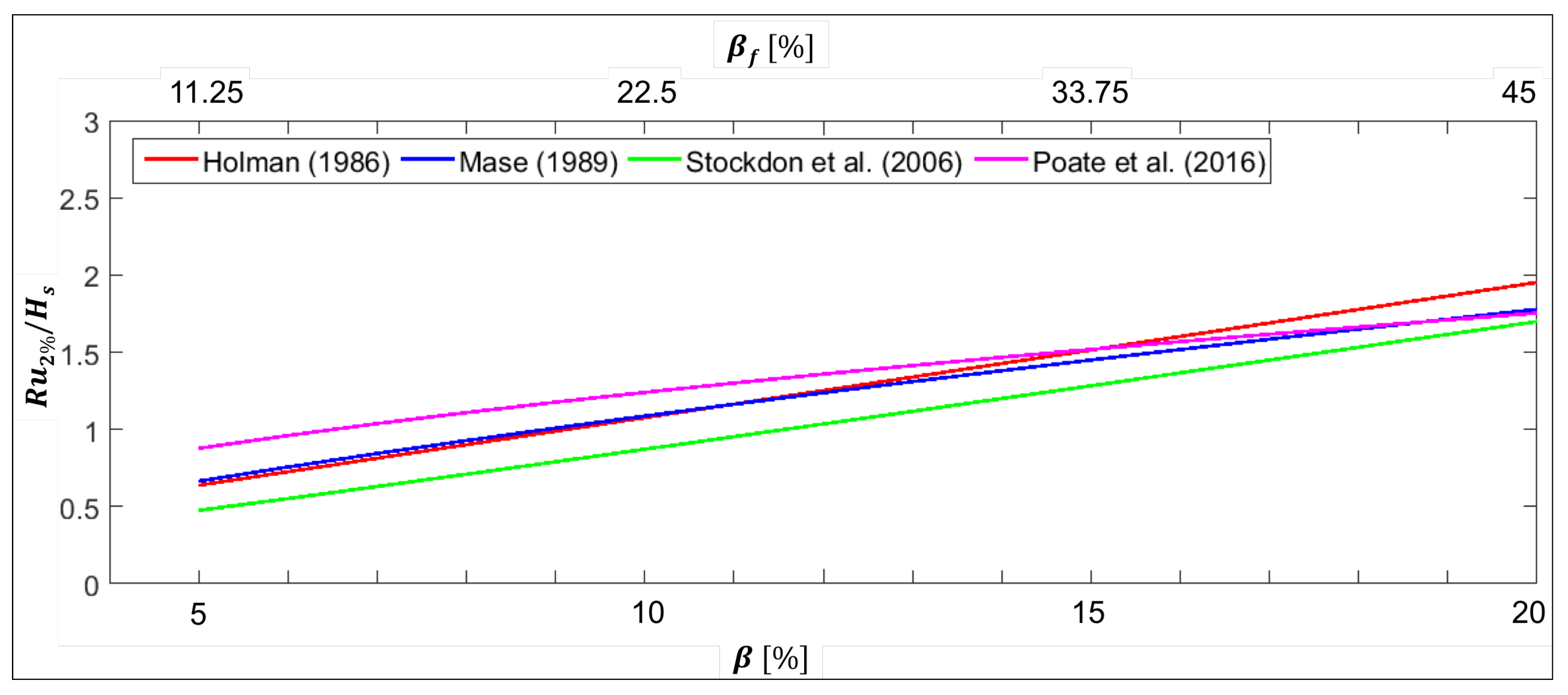
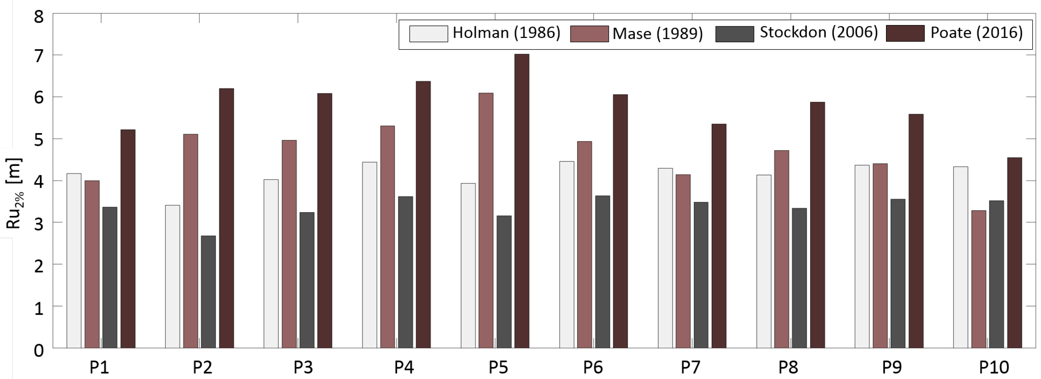
4.3.1. Wave Run-Up Levels and Inundation Distances Obtained by Different Equations.

The different behaviour of the run-up Ru2% formulas, with reference to the case study (February 2014 storm), is reported in Figure 6 as a function of the total beach slope β (used in Mase [14] and Poate et al. [15] equations) and the foreshore slope β f (in Holman [12] and Stockdon et al. [13] equations), in which the β f parameter has been given as a multiple of β .
The examination of Figure 6 shows that, for examined wave conditions, the Poate et al. [15] equation is an upper limit for Ru2% for beaches with a maximum slope of 15%. In this range, the Holman [12] and Mase [14] equations give intermediate and similar results, while the Stockdon et al. [13] equation represents the lower limit. For slopes higher than 15%, Holman [12] and Stockdon et al. [13] represent the higher and lower limit, respectively.
In order to provide evidence of the sensitivity of the run-up level Ru2% to the different equations, this parameter has been reported in Figure 7 for the different transects on the beach. According to the results of Figure 6, the Poate et al. [15] values are the highest in all transects, followed by the Mase [14] and Holman [12] results for transects P2, P3, P4, P5, P6, P8 and P9, and by the Holman [12] and Mase [14] results for transects P1, P7 and P10. The Stockdon et al. [13] results are the lowest, except in profile P10, where they are higher than Mase [14].
The general trend of similarity between the Holman [12] and Mase [14] results is interrupted in transects P2, P3, P4, P5 and P10 in which the ratio β f/ β is different from the one in Figure 7.
The results in terms of floading distance Xmax, normalized with the width of the emerged beach, reported in Figure 8, closely follow those of Ru2%. In particular, for transects P5, P7, P8 and P9, the beach is completely flooded regardless of which formula is considered, while in transects P1, P6 and P10, the maximum Xmax is obtained with the Poate et al. [15] equation and the minimum one with the Stockdon et al. [13] equation. In terms of IRu, the use of Stockdon et al. [13] or Poate et al. [15] equation increases the classification by one score in transects P1 and P6 (from 2 to 3), and in transects P2, P4 and P10 (from 3 to 4).

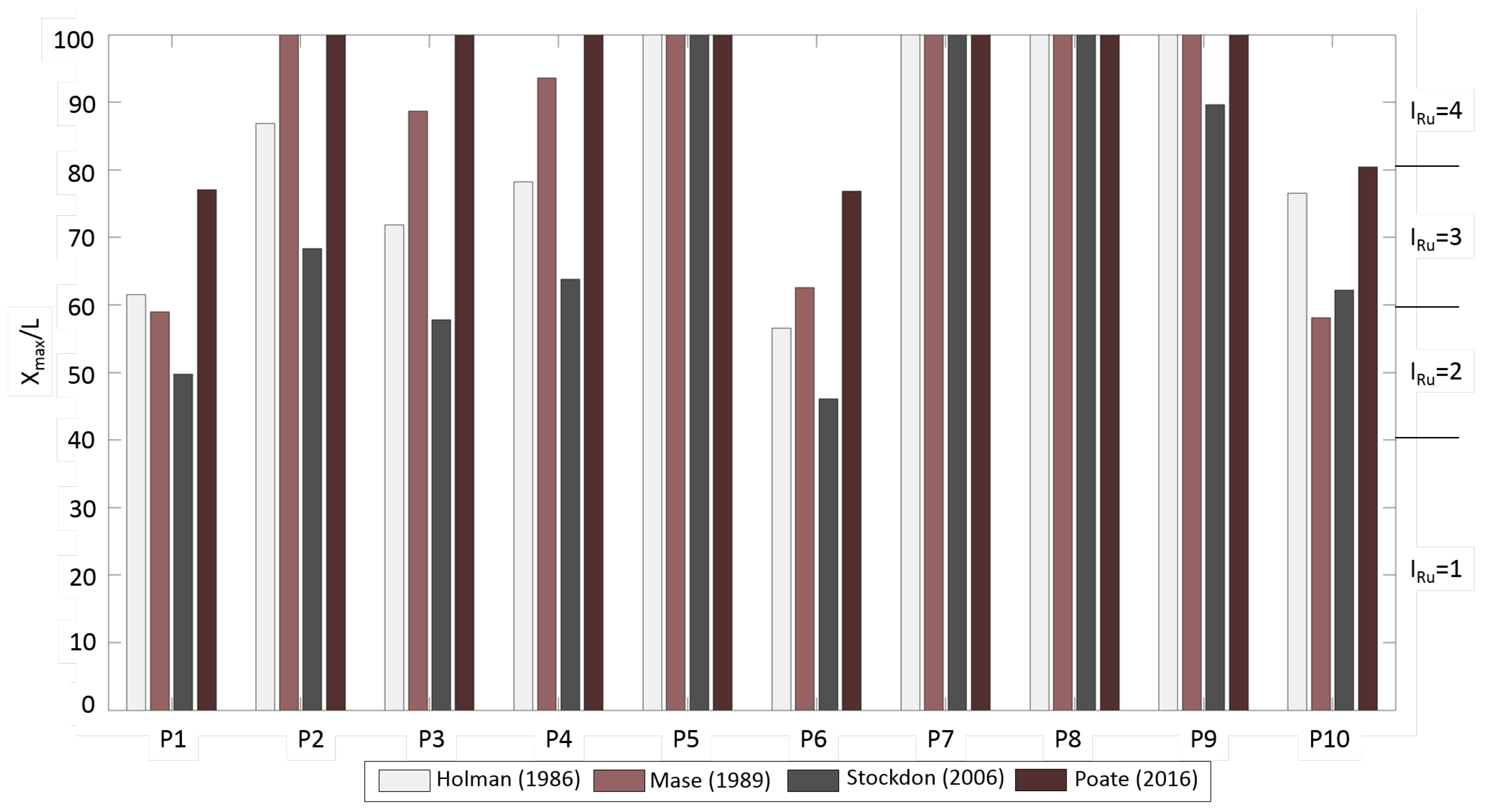
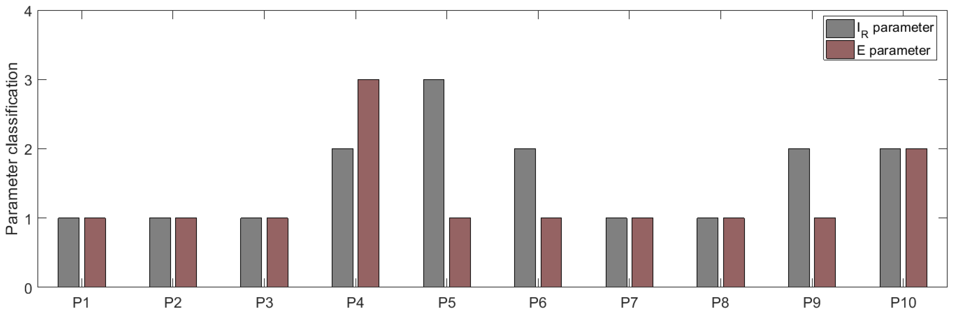
4.3.2. Evaluation of IR, E and ID

According to Equations (8) and (9), the short-term erosion index IR shows a maximum in P5, followed by P6, P9 and P10, due to the limited beach width and smaller grain sizes (Figure 9). Finally, according to the results presented in Table 4, maximum values of E are found in P4, corresponding to the archaeological site.
The ID parameter, linked to the presence and efficiency of coastal defences, assumes −2 score in transects P4, P7 and P8, according to the Kt values calculated considering Equation (10). The coastal structures in P7 and P8, constructed in 2008, demonstrated their efficiency in favoring the beach stability, while the submerged structure in P4 has only recently been realized (see Section 5).

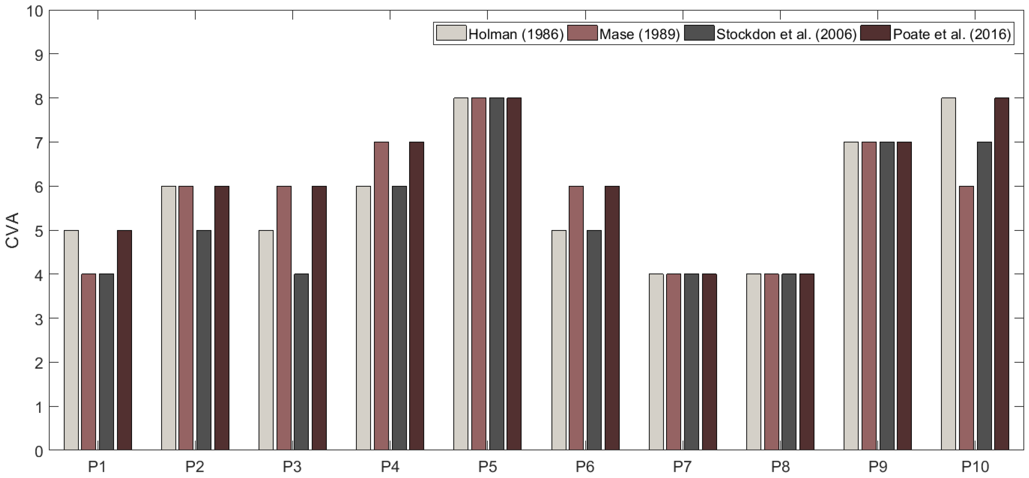
4.4. CVA Sensitivity to the Different Wave Run-Up Formulas

The calculation of CVA on the examined transects was performed following the classification given in Table 2 and was reported in Figure 10. In agreement with IRu results shown in Figure 8, the same value of CVA regardless of the different run-up formulas is reached for the transects P5, P7, P8 and P9. For transects P1, P2, P4, P6 and P10, the use of the Poate et al. [15] equation instead of Stockdon et al. [13] for Ru2% raises the CVA score by one class, while, for transect P3, the difference is sufficient to change the CVA score by two classes.

5. Adaptation Strategy

Starting from the obtained results on coastal inundation and erosion, we propose an adaptation strategy in order to decrease the vulnerability in front of the archaeological area. The protection is obtained through a longitudinal submerged breakwater (Figure 11), located offshore of transect P4. The breakwater has a submerged berm width of approx. 12 m, a crest height of −0.50 m a.s.l. and an overall longitudinal extension of 460 m.
Moreover, a beach nourishment is proposed between transects P3 and P5 for a total extension of approx. 800 m, with an additional beach width of 15 m and a grain size of 5 mm. In order to promote the stabilization of the beach nourishment and obtain a natural beach recovery, a beach drainage system could be also taken into account [50,51]. The residual energy calculation for the breakwater provides a value of 0.47 for the transmission coefficient Kt, with a consequent ID index of −2, like the previous submerged structures realized in front of the transects P7 and P8. These structures lower by two units the CVA score in P4, P7 and P8 profiles, based on the cited Kt value (see Table 2). The defense of the cliff on which the archaeological site is located is obtained by means of an adherent structure.

6. Discussion

The behaviour of the different run-up equations show that the Poate et al. [15] and Stockdon et al. [13] equations give the highest and lowest run-up values, respectively, in all transects, while the Mase [14] and Holman [12] run-up values are intermediate.
The sensitivity of CVA to the different run-up equations cannot be noted for the transects characterized by a lower values of beach width and slope (e.g., P5, P7, P8 and P9 in Figure 10) that are always completely inundated. This is the reason why the different performance of the run-up equations can be made most evident for profiles P2, P3 and P4, where the IRu trend closely follows the Ru2% results. The results show that the run-up obtained by Poate et al. [15] and Mase [14] equations are the highest, giving rise to high inundation percentage, followed by the values obtained by Holman [12] and Stockdon et al. [13]. Similar results are found for P1, P6 and P10, with lower IRu values due to a greater beach width, while, in the remaining profiles P5, P7, P8 and P9, the influence of the different Ru2% formulas is masked by lower values of beach width and slope, which lead to inundation of the whole beach regardless of the used formula.
The mitigation proposal for the most vulnerable transect in front of the archaeological area, consisting of submerged breakwater, decreases the CVA score in P4 transect through a negative value of the index ID, in agreement with Martinelli et al. [10]. The additional defence of the adherent gabion wall facing the cliff, as well as the increase in beach width provided by the beach nourishment in front of transects P3, P4 and P5 (which decrease both indexes IRu and IR) was not taken into account for precautionary reasons.

7. Conclusions

In this paper, the sensitivity of the coastal vulnerability assessment to different wave run-up formulas was examined with reference to a micro-tidal beach in front of an archaeological site. First, we implemented offshore wave simulations based on a WWIII model and validated them by in situ measurements. Then, we configured the run-up calculations with different well known formulas to obtain different run-up levels and examine their influence on CVA calculations. Finally, we proposed a mitigation strategy for the most vulnerable areas, consisting in submerged breakwater for the area facing the archaeological ruins, coupled with an adherent structure for the cliff defence. The following results were obtained:
  • The Poate et al. [15] and the Stockdon et al. [13] equations provide a higher and lower limit, respectively, for run-up levels.
  • The run-up differences are less evident in CVA evaluation, nevertheless they can lead to different CVA scores, except in the case of limited beach width where the transects are completely inundated, regardless of the used run-up empirical formula.
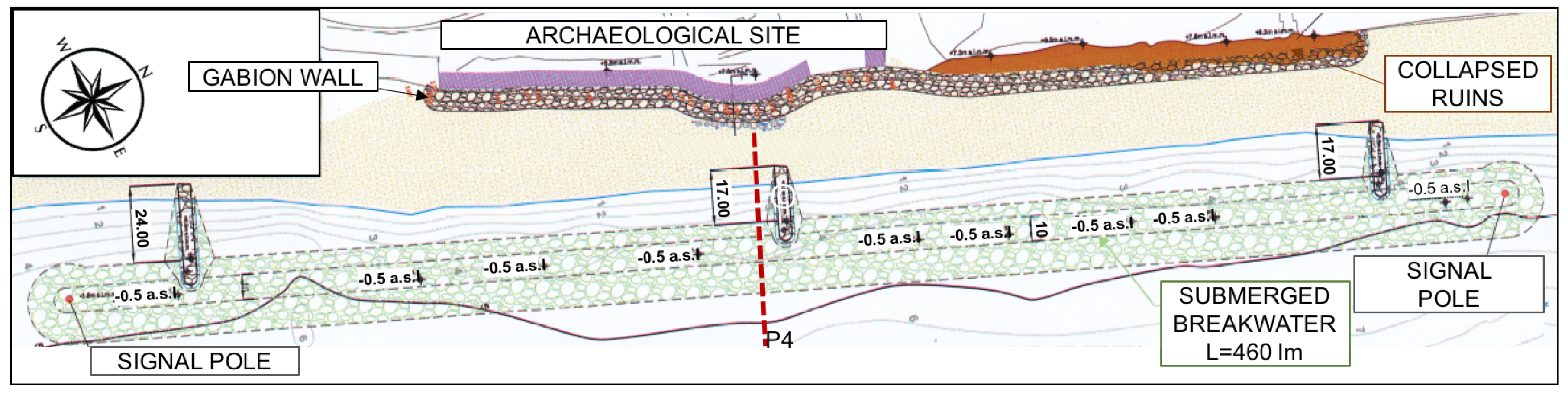
  • The vulnerability mitigation proposal, consisting of a submerged breakwater for the beach protection, decreased the CVA score based on the Kt value.
  • The CVA additional decrease due to an adherent gabion wall for the cliff defense and the artificial nourishment placed in front of the Kaulonia site for a longitudinal extension of 800 m was not taken into account for precautionary reasons.

Author Contributions

Conceptualization, C.M.R. and G.B.; Data Curation, D.D.L., P.C. and G.D.P.; Methodology, G.B., G.D.P. and C.M.R.; Software, R.M., D.D.L. and G.D.P.; Validation, D.D.L. and L.M.; Writing–Original Draft Preparation, C.M.R., G.D.P., D.D.L. and G.B.; Writing–Review & Editing, D.D.L., L.M., G.B., C.M.R., P.C. and G.D.P.

Acknowledgments

The authors are grateful to the CCMMMA (Campania Center for Marine and Atmospheric Monitoring and Modelling, http://meteo.uniparthenope.it), the forecast service of the University of Napoli “Parthenope” for the real-time monitoring and forecast of marine, weather and air quality conditions in the Mediterranean area. The CCMMMA provided the hardware and software resources for the offshore numerical simulations.

Conflicts of Interest

The authors declare no conflict of interest.

References

  1. Gornitz, V. Global coastal hazards from future sea level rise. Palaeogeogr. Palaeoclimatol. Palaeoecol. 1991, 89, 379–398. [Google Scholar] [CrossRef]
  2. De Leo, F.; Besio, G.; Zolezzi, G.; Bezzi, M. Coastal vulnerability assessment: through regional to local downscaling of wave characteristics along the Bay of Lalzit (Albania). Nat. Hazards Earth Syst. Sci. Discuss. 2018, 2018, 1–19. [Google Scholar] [CrossRef] [Green Version]
  3. Besio, G.; Donini, L.; Gallini, S.; Onorato, L. A prompt index for sea storm hazard. In Proceedings of the 7th Short Course and Conference on Applied Coastal Research (SCACR), Florence, Italy, 28 September–1 October 2015; pp. 553–560. [Google Scholar]
  4. Di Paola, G.; Aucelli, P.P.C.; Benassai, G.; Rodríguez, G. Coastal vulnerability to wave storms of Sele littoral plain (southern Italy). Nat. Hazards 2014, 71, 1795–1819. [Google Scholar] [CrossRef]
  5. Tragaki, A.; Gallousi, C.; Karymbalis, E. Coastal Hazard Vulnerability Assessment Based on Geomorphic, Oceanographic and Demographic Parameters: The Case of the Peloponnese (Southern Greece). Land 2018, 7, 56. [Google Scholar] [CrossRef]
  6. Mavromatidi, A.; Briche, E.; Claeys, C. Mapping and analyzing socio-environmental vulnerability to coastal hazards induced by climate change: An application to coastal Mediterranean cities in France. Cities 2018, 72, 189–200. [Google Scholar] [CrossRef]
  7. Di Paola, G.; Aucelli, P.P.C.; Benassai, G.; Iglesias, J.; Rodríguez, G.; Rosskopf, C.M. The assessment of the coastal vulnerability and exposure degree of Gran Canaria Island (Spain) with a focus on the coastal risk of Las Canteras Beach in Las Palmas de Gran Canaria. J. Coast. Conserv. 2017, 1–15. [Google Scholar] [CrossRef]
  8. Benassai, G.; Di Paola, G.; Aucelli, P.P.C. Coastal risk assessment of a micro-tidal littoral plain in response to sea level rise. Ocean Coast. Manag. 2015, 104, 22–35. [Google Scholar] [CrossRef]
  9. Aucelli, P.P.C.; Di Paola, G.; Incontri, P.; Rizzo, A.; Vilardo, G.; Benassai, G.; Buonocore, B.; Pappone, G. Coastal inundation risk assessment due to subsidence and sea level rise in a Mediterranean alluvial plain (Volturno coastal plain—southern Italy). Estuar. Coast. Shelf Sci. 2017, 198, 597–609. [Google Scholar] [CrossRef]
  10. Martinelli, L.; Zanuttigh, B.; Corbau, C. Assessment of coastal flooding hazard along the Emilia Romagna littoral, IT. Coast. Eng. 2010, 57, 1042–1058. [Google Scholar] [CrossRef]
  11. Battjes, J.A. Surf similarity. In Coastal Engineering 1974; American Society of Civil Engineers: Reston, VA, USA, 1975; pp. 466–480. [Google Scholar]
  12. Holman, R. Extreme value statistics for wave run-up on a natural beach. Coast. Eng. 1986, 9, 527–544. [Google Scholar] [CrossRef]
  13. Stockdon, H.F.; Holman, R.A.; Howd, P.A.; Sallenger, A.H. Empirical parameterization of setup, swash, and runup. Coast. Eng. 2006, 53, 573–588. [Google Scholar] [CrossRef]
  14. Mase, H. Random wave runup height on gentle slope. J. Waterw. Port Coast. Ocean Eng. 1989, 115, 649–661. [Google Scholar] [CrossRef]
  15. Poate, T.G.; McCall, R.T.; Masselink, G. A new parameterisation for runup on gravel beaches. Coast. Eng. 2016, 117, 176–190. [Google Scholar] [CrossRef]
  16. Montella, R.; Giunta, G.; Riccio, A. Using grid computing based components in on demand environmental data delivery. In Proceedings of the Second Workshop on Use of P2P, GRID and Agents for the Development of Content Networks, Monterey, CA, USA, 25 June 2007; ACM: New York, NY, USA, 2007; pp. 81–86. [Google Scholar]
  17. Benassai, G.; Ascione, I. Implementation and validation of wave watch III model offshore the coastlines of southern Italy. In Proceedings of the 25th International Conference on Offshore Mechanics and Arctic Engineering, Hamburg, Germany, 4–9 June 2006; pp. 553–560. [Google Scholar] [CrossRef]
  18. Benassai, G.; Ascione, I. Implementation of WWIII wave model for the study of risk inundation on the coastlines of Campania, Italy. WIT Trans. Ecol. Environ. 2006, 88. [Google Scholar] [CrossRef] [Green Version]
  19. Benassai, G.; Aucelli, P.; Budillon, G.; De Stefano, M.; Di Luccio, D.; Di Paola, G.; Montella, R.; Mucerino, L.; Sica, M.; Pennetta, M. Rip current evidence by hydrodynamic simulations, bathymetric surveys and UAV observation. Nat. Hazards Earth Syst. Sci. 2017, 17, 1493–1503. [Google Scholar] [CrossRef] [Green Version]
  20. Arena, G.; Briganti, R.; Corsini, S.; Franco, L. The Italian wave measurement buoy network: 12 years management experience. In Ocean Wave Measurement and Analysis (2001); American Society of Civil Engineers: Reston, VA, USA, 2002; pp. 86–95. [Google Scholar] [CrossRef]
  21. Di Paola, G.; Iglesias, J.; Rodríguez, G.; Benassai, G.; Aucelli, P.; Pappone, G. Estimating coastal vulnerability in a meso-tidal beach by means of quantitative and semi-quantitative methodologies. J. Coast. Res. 2011, 303–308. [Google Scholar] [CrossRef]
  22. Benassai, G.; Di Paola, G.; Aucelli, P.; Passarella, M.; Mucerino, L. An inter-comparison of coastal vulnerability assessment methods. In Engineering Geology for Society and Territory-Volume 4; Springer: Berlin, Germany, 2014; pp. 45–49. [Google Scholar] [CrossRef]
  23. Benassai, G.; Migliaccio, M.; Montuori, A.; Ricchi, A. Wave Simulations Through Sar Cosmo-Skymed Wind Retrieval and Verification with Buoy Data. In Proceedings of the Twenty-Second International Offshore and Polar Engineering Conference, Rhodes, Greece, 17–22 June 2012. ISOPE-I-12-426. [Google Scholar]
  24. Benassai, G.; Montuori, A.; Migliaccio, M.; Nunziata, F. Sea wave modeling with X-band COSMO-SkyMed? SAR-derived wind field forcing and applications in coastal vulnerability assessment. Ocean Sci. 2013, 9, 325. [Google Scholar] [CrossRef]
  25. D’Alessandro, L.; Davoli, L.; Lupia Palmieri, E.; Raffi, R. Natural and anthropogenic factors affecting the recent evolution of beaches in Calabria (Italy). In Applied Geomorphology: Theory and Practice; John Wiley & Sons Ltd.: Chichester, UK, 2002; pp. 397–427. [Google Scholar]
  26. Terranova, O.; Gariano, S. Rainstorms able to induce flash floods in a Mediterranean-climate region (Calabria, southern Italy). Nat. Hazards Earth Syst. Sci. 2014, 14, 2423. [Google Scholar] [CrossRef]
  27. Calabria, R. Master Plan Erosione Costiera—Autorità di Bacino Regionale—Area 9. 2013. Available online: http://old.regione.calabria.it/abr/index.php?option=com_content&task=view&id=428&Itemid=282 (accessed on 1 June 2018).
  28. Goda, Y. On the methodology of selecting design wave height. In Coastal Engineering 1988; American Society of Civil Engineers: Reston, VA, USA, 1989; pp. 899–913. [Google Scholar] [CrossRef]
  29. Mathiesen, M.; Goda, Y.; Hawkes, P.J.; Mansard, E.; Martín, M.J.; Peltier, E.; Thompson, E.F.; Van Vledder, G. Recommended practice for extreme wave analysis. J. Hydraul. Res. 1994, 32, 803–814. [Google Scholar] [CrossRef]
  30. Hershfield, D.; Kohler, M. An empirical appraisal of the Gumbel extreme-value procedure. J. Geophys. Res. 1960, 65, 1737–1746. [Google Scholar] [CrossRef]
  31. Carter, D.; Challenor, P. Methods of fitting the Fisher–Tippett Type 1 extreme value distribution. Ocean Eng. 1983, 10, 191–199. [Google Scholar] [CrossRef]
  32. Stanley, J.D.; Bernasconi, M.P. Buried and submerged Greek archaeological coastal structures and artifacts as gauges to measure late Holocene seafloor subsidence off Calabria, Italy. Geoarchaeology 2012, 27, 189–205. [Google Scholar] [CrossRef]
  33. ISPRA. Data Analysis. 2014. Available online: http://www.idromare.it/analisi_dati.php (accessed on 10 October 2014).
  34. ASTM D421-85(2007). Standard Practice for Dry Preparation of Soil Samples for Particle-Size Analysis and Determination of Soil Constants. Available online: http://www.astm.org/Standards/D421.htm (accessed on 17 November 2014).
  35. ASTM D422 (Hydrometer). Standard test method for particle-size analysis of soils. In Annual Book of ASTM Standards; ASTM International: West Conshohocken, PA, USA, 2007; Available online: http://www.astm.org/Standards/D421.htm (accessed on 17 November 2014).
  36. Giunta, G.; Montella, R.; Mariani, P.; Riccio, A. Modeling and computational issues for air/water quality problems: A grid computing approach. Nuovo Cimento C Geophys. Space Phys. C 2005, 28, 215. [Google Scholar] [CrossRef]
  37. CCMMMA, Campania Center for Marine and Atmospheric Monitoring and Modelling. Available online: meteo.uniparthenope.it (accessed on 1 April 2009).
  38. Di Lauro, R.; Giannone, F.; Ambrosio, L.; Montella, R. Virtualizing general purpose GPUs for high performance cloud computing: An application to a fluid simulator. In Proceedings of the 2012 IEEE 10th International Symposium on Parallel and Distributed Processing with Applications (ISPA), Leganes, Spain, 10–13 July 2012; pp. 863–864. [Google Scholar] [CrossRef]
  39. Montella, R.; Coviello, G.; Giunta, G.; Laccetti, G.; Isaila, F.; Blas, J.G. A general-purpose virtualization service for HPC on cloud computing: An application to GPUs. In Parallel Processing and Applied Mathematics; Springer: Berlin, Germany, 2011; pp. 740–749. [Google Scholar] [CrossRef]
  40. Skamarock, W.C.; Klemp, J.B. A time-split nonhydrostatic atmospheric model for weather research and forecasting applications. J. Comput. Phys. 2008, 227, 3465–3485. [Google Scholar] [CrossRef]
  41. Michalakes, J.; Dudhia, J.; Gill, D.; Henderson, T.; Klemp, J.; Skamarock, W.; Wang, W. The weather research and forecast model: software architecture and performance. In Use of High Performance Computing in Meteorology; World Scientific: Singapore, 2005; pp. 156–168. [Google Scholar] [CrossRef]
  42. Tolman, H.L.; Chalikov, D. Source terms in a third-generation wind wave model. J. Phys. Oceanogr. 1996, 26, 2497–2518. [Google Scholar] [CrossRef]
  43. Tolman, H.L. User manual and system documentation of WAVEWATCH III TM version 3.14. Tech. Note MMAB Contrib. 2009, 276, 220. [Google Scholar]
  44. Kriebel, D.L.; Dean, R.G. Convolution method for time-dependent beach-profile response. J. Waterw. Port Coast. Ocean Eng. 1993, 119, 204–226. [Google Scholar] [CrossRef]
  45. D’Angremond, K.; Van Der Meer, J.W.; De Jong, R.J. Wave transmission at low-crested structures. In Coastal Engineering 1996; American Society of Civil Engineers: Reston, VA, USA, 1997; pp. 2418–2427. [Google Scholar] [CrossRef]
  46. Martínez del Pozo, J.; Anfuso, G. Spatial approach to medium-term coastal evolution in south Sicily (Italy): Implications for coastal erosion management. J. Coast. Res. 2008, 33–42. [Google Scholar] [CrossRef]
  47. Thieler, E.R.; Himmelstoss, E.A.; Zichichi, J.L.; Ergul, A. The Digital Shoreline Analysis System (DSAS) Version 4.0—An ArcGIS Extension for Calculating Shoreline Change; Technical Report; US Geological Survey: Reston, VA, USA, 2009.
  48. Mentaschi, L.; Besio, G.; Cassola, F.; Mazzino, A. Developing and validating a forecast/hindcast system for the Mediterranean Sea. J. Coast. Res. 2013, 65, 1551–1556. [Google Scholar] [CrossRef]
  49. Melby, J.; Caraballo-Nadal, N.; Kobayashi, N. Wave runup prediction for flood mapping. Coast. Eng. Proc. 2012, 1, 79. [Google Scholar] [CrossRef]
  50. Ciavola, P.; Vicinanza, D.; Aristodemo, F.; Contestabile, P. Large-scale morphodynamic experiments on a beach drainage system. J. Hydraul. Res. 2011, 49, 523–528. [Google Scholar] [CrossRef]
  51. Contestabile, P.; Aristodemo, F.; Vicinanza, D.; Ciavola, P. Laboratory study on a beach drainage system. Coast. Eng. 2012, 66, 50–64. [Google Scholar] [CrossRef]
Figure 1. Google EarthTM images (Image©2016 Digital Globe) of the study area (a); and a view from above of part of the archeological area of Kaulonia (b); view of a small strip of the beach in front of the archeological area (c).
Sustainability 10 02017 g001
Figure 2. Main and secondary fetches (Google EarthTM product) (a) geographical fetches (limited to 500 km) and effective fetch (b); directional distribution of Hs and main fetch subdivision (c).
Sustainability 10 02017 g002
Figure 3. Beach profiles P1–P10 (a) and views of the beach in correspondence of transects P1, P3, P4, P7, P8 and P10 (b).
Sustainability 10 02017 g003
Figure 4. Annual shoreline change rates (m/yr) of the study beach for periods 1958–2014 (a) and 1996–2014 (b). The x-axis shows the analyzed coastal stretch together with DSAS (Digital Shoreline Analysis System) transects.
Sustainability 10 02017 g004
Figure 5. Simulated Hs distribution on d02 (Italy) computational domain (a) and a zoomed-in version on the Ionian sea (b); comparison of simulated (black line) and recorded (red line) waves during the February 2014 sea storm (c).
Sustainability 10 02017 g005
Figure 6. Ru2%/Hs as a function of β for the different equations with reference to the February 2014 storm.
Sustainability 10 02017 g006
Figure 7. Run-up levels obtained by the different equations with reference to the February 2014 storm.
Sustainability 10 02017 g007
Figure 8. Maximum normalized inundation distance and relative run-up index obtained by the different run-up equations.
Sustainability 10 02017 g008
Figure 9. IR and E classification obtained for the transects P1–P10.
Sustainability 10 02017 g009
Figure 10. Coastal Vulnerability Assessment (CVA) obtained by the different run-up equations.
Sustainability 10 02017 g010
Figure 11. Coastal vulnerability mitigation proposal in front of the archaeological site. The dotted red line is the beach transect P4 located in front of the archaeological site.
Sustainability 10 02017 g011
Table 1. Extreme wave heights corresponding to different return periods for each homogeneous sector calculated using the Gumbel (Fisher–Tippett I) cumulative probability distribution function [30,31]. HTr is the wave height for different return period Tr and yr is the relative reduced variable.
Tr (yr)SectoryrHTr (m)Tr (yr)SectoryrHTr (m)
1S2a3.325.0020S2a6.337.50
S2b3.775.95S2b6.788.74
S2c3.973.37S2c6.984.58
5S2a4.946.3550S2a7.258.26
S2b5.397.45S2b7.699.59
S2c5.594.02S2c7.894.95
10S2a5.646.93100S2a7.948.84
S2b6.098.10S2b8.3910.23
S2c6.294.30S2c8.595.23
Table 2. Scores associated with each variable for CVA (Coastal Vulnerability Assessment) evaluation.
ParameterClassification
1234
IR(%)<1515–3030–50>50
IRu(%)<4040–6060–80>80
E (m/yr)<−0.5−0.5–−1.0−1.0–−2.0>−2.0
ID−1−2−3−4
Kt>0.580.41–0.580.24–0.41<0.24
Table 3. Grain size and morphological features of the backshore and foreshore zones along profiles P1–P10.
ProfileBackshore Width
L (m)
Backshore Slope
βb (%)
Foreshore Slope
βf (%)
Total Slope
β (%)
Foreshore Median
Sediment Diameter
μ (mm)
P136.86.118.47.55.18
P227.69.614.210.66.12
P331.88.617.610.25.96
P428.59.719.911.23.45
P513.310.517.113.62.55
P639.48.920.010.14.66
P717.65.719.17.95.93
P810.02.618.29.54.70
P920.36.119.58.62.80
P1029.33.119.35.72.62
Table 4. Total and mean annual shoreline variations along profiles P1–P10 during the periods 1958–2014 and 1996–2014.
PeriodShoreline VariationP1P2P3P4P5P6P7P8P9P10
1958–2014Total (m)−25.43−8.49−38.46−38.17−24.04−6.61−5.97−43.25−60.67−54.86
Annual mean (m/yr)−0.43−0.65−0.65−0.65−0.41−0.28−0.10−0.73−1.03−0.93
1996–2014Total (m)6.90−0.897.74−33.26−9.3616.4612.1223.3227.19−9.96
Annual mean (m/yr)0.37−0.05−0.42−1.80−0.510.890.651.261.47−0.53
Table 5. Statistical indices, obtained according with Mentaschi et al. [48] and Melby et al. [49], for comparison between simulated and recorded wave of the February 2014 storm (Figure 5c). R = correlation index; BI = normalized bias; SI = normalized scatter index; RMSE = root mean square error; NRMSE = normalized root mean square error; BIP = BI performance; SIP = SI performance; NRMSEP = NRMSE Performance; SPS = Summary Performance Score.
RBISIRMSENRMSEBIPSIPNRMSEPSPS
Hs0.9330.0530.1350.4960.1440.9470.8650.8560.889
Tm0.6720.2200.1861.7060.2830.7790.8150.7170.771
Dm0.826−0.0420.10515.9650.1130.9580.8960.8880.914

