Post-Earthquake Restoration Simulation Model for Water Supply Networks

1
Department of Civil Engineering, Kyung Hee University, Yongin-si, Gyeonggi-do 17104, Korea
2
Department of Civil Engineering, The University of Suwon, Hwaseong-si, Gyeonggi-do 18323, Korea
3
Department of Civil Engineering, Kyung Hee University, 1732 Deogyeong-daero, Giheung-gu, Yongin-si, Gyeonggi-do 17104, Korea
*
Author to whom correspondence should be addressed.
Sustainability 2018, 10(10), 3618; https://0-doi-org.brum.beds.ac.uk/10.3390/su10103618
Submission received: 7 September 2018
/
Revised: 27 September 2018
/
Accepted: 8 October 2018
/
Published: 10 October 2018
(This article belongs to the Special Issue Resilience and Sustainability of Civil Infrastructures under Extreme Loads)
Abstract
:A computer-based simulation model was developed to quantify the seismic damage that may occur in water supply networks and to suggest restoration strategies after such events. The model was designed to produce probabilistic seismic events and determine the structural damage of facilities. Then, the model numerically quantifies the system restoration rate over time by connecting it with a hydraulic analysis solver. The model intends to propose superb restoration plans by performing sensitivity analyses using several restoration scenarios. The developed model was applied to an actual metropolitan waterworks system currently operating in South Korea and successfully suggested the most efficient restoration approaches (given seismic damage) to minimize the complete recovery time and suspension of water service. It is expected that the proposed model can be utilized as a decision-making tool to determine prompt system recovery plans and restoration priorities in the case of an actual seismic hazard that may occur in water supply networks.
1. Introduction
A water supply network is a human-made infrastructure supplying drinking water. If it partially or completely loses water supply function because of an unforeseen disaster, massive social and economic damage may result. Therefore, consistent maintenance to prevent such a setback in water service is critical. In general, there are several factors that inhibit such function, including the physical deterioration of network facilities (pipelines in particular), human-made hazards resulting in pipeline damage during ground construction, and natural disasters such as earthquakes and floods. Among them, natural disasters are beyond human control, and the extent of damage can be catastrophic. Thus, natural disasters require preemptive maintenance compared to other factors. Among other types of natural disasters, earthquakes have the most significant and direct impact on the water supply network because most components are buried underground.
In general, the approaches used to reduce seismic damage can be largely divided into two branches. The first one is reinforcing system durability to prevent damage or to minimize the immediate deterioration of a system. Because it is difficult to predict the exact timing of an earthquake event, it would be beneficial to develop an earthquake-resistant system through advanced reinforcement or system design [1,2]. The second approach is to enhance the resiliency of the system by post-earthquake restoration. Because the natural disasters are not entirely preventable, improving system resiliency in terms of post-event restoration is essential to avoid long-term losses.
Several representative seismic damage quantification models of water supply systems include (1) HAZUS developed by the Federal Emergency Management Agency [3]; (2) MAEviz [4] developed at the Mid-America Earthquake Center; (3) GIRAFFE (Graphical Iterative Response Analysis of Flow Following Earthquakes) introduced by Shi et al. [5]; and (4) REVAS.NET (Reliability EVAluation model for seismic hazard for water supply NETwork) created by Yoo [6]. HAZUS and MAEviz are computer models that quantify the damage occurred in social infrastructures in terms of societal and economic value and do not include restoration measures nor simulation of system performance. GIRAFFE and REVAS.NET present the extent of earthquake damage on water supply networks by quantifying the water supply capacity or system serviceability. These two models are capable of hydraulic analysis via linkage to a hydraulic solver; however, GIRAFFE lacks of hydraulic module to depict a detailed hydraulic behavior of the damaged water networks and REVAS. NET is mainly intended to estimate system reliability against seismic damage. They are not equipped to simulate the detailed post-earthquake restoration process.
Other studies that quantified the earthquake damage to water supply networks include Adachi and Ellingwood [7], and Yoo et al. [8]. Adachi and Ellingwood [7] claimed that water pipe networks and power systems should be evaluated jointly for more accurate assessment of system serviceability when seismic damage occurred to water pipe networks. Yoo et al. [8] quantified the serviceability of water supply system during an earthquake and proposed optimal design measures to reinforce the system. Those studies quantified the serviceability of water supply systems under seismic damage, but no applications for the post-event restoration simulation were provided.
In addition, Davenport et al. [9], Tabucchi et al. [10], and Luna et al. [11] published studies related to the reinforcement of post-earthquake system stability. These studies suggested various methods of restoring water pipe networks to a normal (or close to normal) state after an earthquake, but did not include any hydraulic analysis modules to simulate water supplies within an actual water pipe network in the event of a disaster. Recently, Tabucchi et al. [12] modeled a series of processes where various types of recovery support staffs were assigned to repair the system, and evaluated hydraulic performance of a system using a GIRAFFE model. The developed model was verified by simulating the 1994 Northridge earthquake that occurred in Los Angeles, California. The study demonstrated that the sequence and phases of a restoration process can be estimated accurately through modeling but did not attempt to propose and evaluate diverse recovery measures.
Lately, Davis et al. [13], Davis [14], and Davis and Giovinazzi [15] subdivided the serviceability of a water pipe network into several factors, such as “water delivery,” “quality,” “quantity,” “fire protection,” and “functionality.” They showed the quantified recovery phases of each item and analyzed the phases by comparing them with the case of the Northridge earthquake recovery.
Most recently, Klise et al. [16,17] introduced the Water Network Tool for Resilience (WNTR), a new open source Python package designed to help water utilities investigating water service availability (WSA) and recovery time based on earthquake magnitude, location, and repair strategy. Their study mainly focused on introducing the developed model, yet not conducted simulations to compare and analyze diverse restoration strategies suitable to a damaged network.
In summary, the previous studies have limitations in that they lack hydraulic simulations required to describe the hydraulic behavior of damaged water networks and post-event restoration simulations for prompt system recovery. This study focuses on efforts to recover water system service after seismic damage in an efficient way and attempts to simulate the real-life restoration process. To that end, a computer simulation model was developed to simulate diverse damage recovery approaches in a virtual and risk-free environment. The developed model was applied to an actual metropolitan water supply network operating in South Korea and was used to evaluate various recovery strategies and suggest the most efficient scheme for the application network. This paper consists of four sections. Section 2 covers methodologies such as the earthquake and recovery simulations of the model, Section 3 introduces the applied network and the scenario-setting for a sensitivity analysis and compares and analyzes the results of each scenario. Lastly, Section 4 contains the conclusions of the study and provides future research directions.
2. Methodology
2.1. Model Overview
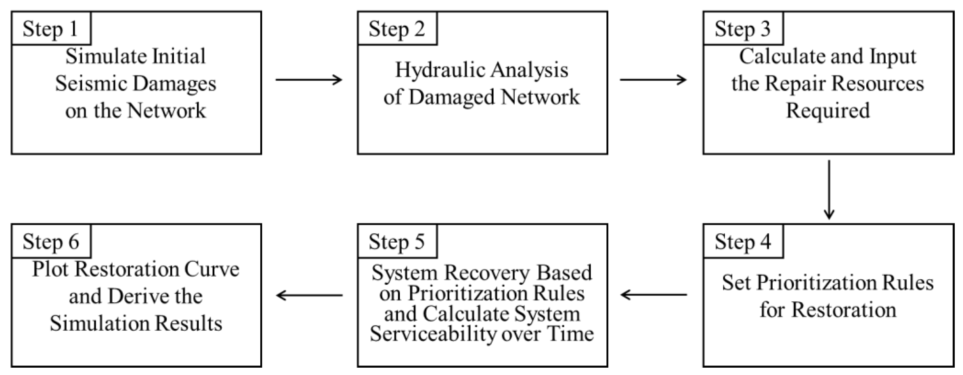
The proposed model was developed using MATLAB [18] in conjunction with a hydraulic solver, EPANET2 [19]. EPANET2 was used to perform hydraulic analyses of water pipe networks, and MATLAB was used to simulate seismic damage of the network and the post-event system restoration processes. The water network components simulated in the model include the pipelines, water storage tanks, and pump facilities. Note that the seismic damages to valves and other facilities were excluded from our simulation. The developed model has six simulation steps as shown in Figure 1, and a brief explanation of each step is provided below.
Step 1. Simulate the initial seismic damage of the network immediately after the earthquake. The damage state of each component (pipelines, pumps, and tanks) is determined based on the seismic location and magnitude.
Step 2. The damage state of the components from Step 1 is provided as the input data of the hydraulic solver (EPANET2), and the hydraulic analysis is conducted to estimate the water supplying condition prior to a system restoration.
Step 3. After the water supply condition is estimated from Step 2, the required recovery resources are calculated and input. Recovery resources include repair crews, equipment, and restoration materials. In this study, only repair personnel were simulated.
Step 4. After entering the available recovery resources, the user sets the recovery priority rules. For example, a pipe carrying higher flow gets priority, or a pipe near a water source (water treatment plant, reservoir, or tank) would be fixed first.
Step 5. The system restoration simulation starts according to the pre-determined recovery plans from Step 4. The system restoration process is monitored over time, and the results are saved in the database. The restoration process is continued until the urgent recovery is completed. Here, the urgent recovery means the repair of the broken pipes. The detection and repair of the leaking pipes occurs subsequently and is not simulated in this study.
Step 6. Once urgent recovery is completed, the recovery strategies are quantitatively evaluated based on various simulation results, such as system restoration curves and recovery crew activity statistics.
2.2. Model Simulation Process
2.2.1. Earthquake Simulation and Damage Determination
(1) Determining Damage to Tanks and Pumps
The model determines the seismic damage to each component by considering the attenuation of the seismic waves, which is estimated based on the distance from the earthquake epicenter and magnitude of the earthquake. The earthquake occurrence time and the location/magnitude are randomly generated and applied. Damage to facilities is caused by the seismic waves after an earthquake occurs, and such waves imply the movement of vibrations from the earthquake, which generally decrease as the distance from the epicenter increases. Such seismic waves affect the estimation of peak ground acceleration (PGA). PGA is an index of how strongly the ground shakes, which directly influences the seismic damage condition. To estimate the PGA, a formula suggested by Baag et al. [20] was implemented as seen in Equation (1).
Here, PGA = peak ground acceleration (), M = magnitude of earthquake, and R = distance (km) from the epicenter assuming a focal depth of 10 km.
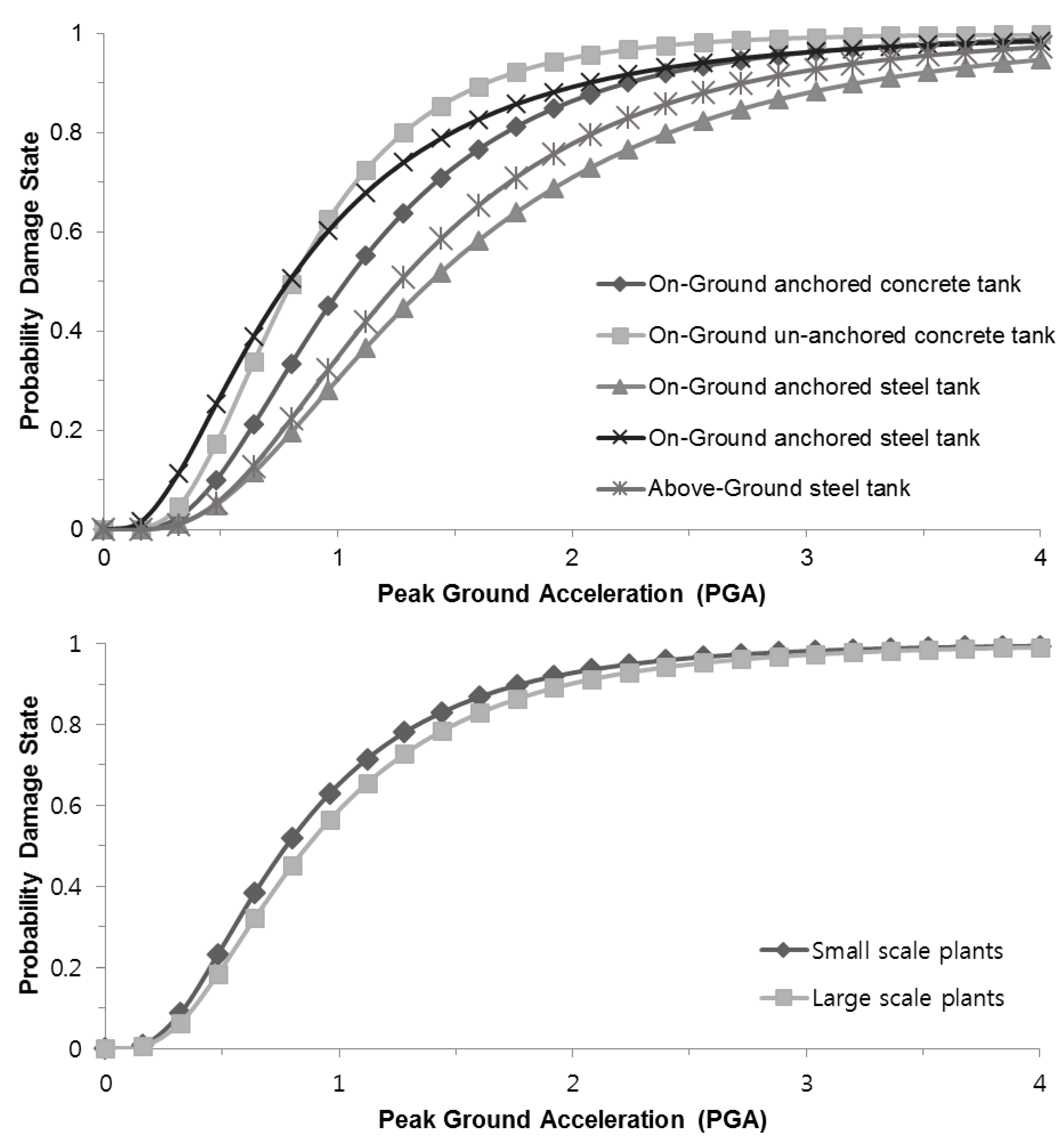
The facility damage caused by an earthquake can be estimated using the fragility curve. The fragility curve shows the probability that the extent of a facility’s damage is beyond a certain level depending on the PGA. The fragility curves presented in the Seismic Fragility Formulations for Water Systems Part 1 Guidelines [21] were applied to determine the damage status of tanks and pumps, as shown in Figure 2. The y-axis indicates the probability that the facility incurs damage when the PGA value of the seismic wave corresponds to the x-axis. The “on-ground anchored concrete tank” and a “small-scale plant” were assumed for the tank and pump types in our model, respectively.
The model classifies the damage of the tank and pump into two states: damaged (function stopped) or normal. The facility damage estimation steps are as follows.
- (1)
- Calculate the PGA of seismic waves that reached each facility using the seismic wave attenuation equation (Equation (1)).
- (2)
- Calculate the damage probability of each facility using the obtained PGA value and the fragility curves (Figure 2).
- (3)
- Generate a random number between 0 and 1 for each facility.
- (4)
- If the random number is smaller than the damage probability derived in step 2, the facility is defined as “damaged”, otherwise, it is “normal”.
The repair time for the damaged facilities was estimated by a random number following a uniform distribution. Note the repair time of a tank is uniformly selected from 24 to 36 h, and that of a pump takes from 8 to 12 h.
(2) Determining Damage to Pipes
In general, damage to a pipeline can be determined based on the concept of repair rate (RR). The repair rate is defined as the number of repairs per unit length of a pipeline and is generally calculated by peak ground velocity (PGV) under seismic event. The American Lifelines Alliance (ALA) [21] suggested the repair rate of a pipe as expressed in Equation (2). The equation was derived based on 81 pipe failure data.
Here, RR = repair rate (no. of repairs/1000ft), K = modification factor
Isoyama [22] has provided various correction factors (C) representing the network information. The correction factors were estimated using the historical seismic data and represent four characteristics, such as pipe diameter, pipe material, topography and soil liquefaction. In this study, Equation (2) was adapted by implementing the correction factors (C) suggested by Isoyama [22] and finally expressed in Equation (3).
Here, , , and represent the correction factors for the pipe diameter, pipe material, topography, and liquefaction, respectively.
To determine the pipe damage status, the Poisson distribution is widely utilized as noted by ALA [21]. To determine the probability of failure of an individual pipeline with a length of L, the Poisson distribution is expressed as:
Here, x is a random variable denotes the number of events (i.e., pipe breaks) and is an average rate of breaks (or repairs) per unit length of pipe (i.e., RR of a pipe).
Since a single break in a pipe takes the entire pipeline out of service, the probability of break of an individual pipeline can be easily calculated by setting k = 0 in Equation (4) and subtracting it from 1. Thus, the probability of pipe failure can be calculated as expressed in Equation (5).
Here, = probability of pipe breakage and = pipe length.
In the model, the seismic damage to pipelines is divided into breakage and leakage. If a pipe is broken, the water flow through the pipe is completely suspended, while a pipe with leaks still conveys water with potential loss of flow and pressure. Here, the pipe damage condition was simulated through the following procedure:
- (1)
- Calculate the PGV value of the seismic wave arriving at each pipe.
- (2)
- Calculate the repair rate of the pipes using Equation (3).
- (3)
- Estimate the distance between repair points of each pipe (L1 = 1/RR) and compare it with the actual pipe length (L2) to determine whether earthquake damage has occurred in the pipe. That is, if L1 is larger than L2, no damage occurs in the pipe.
- (4)
- For the damaged pipe with L1 < L2, a random number between 0 and 1 is generated and compared with the pipe failure probability (Equation (5)). If the random number is smaller than the breakage probability, the pipe is considered to be broken, otherwise it is leaking.
- (5)
- Using this procedure, all the pipes in the network are classified into either ‘no damage’, ‘leakage’ or ‘breakage’.
The repair time of a broken pipe was estimated using the empirical formula suggested by Chang et al. [23] as expressed in Equation (6). The equation was derived by the Korea Water Resources Corporation (K-water) based on a number of field data. Although the repair time may be affected by the accessibility to the repair site, it was found that the repair time is generally proportional to the pipe diameter with a preparation time (2 h) as shown in Equation (6).
Here, = repair time for a broken pipe (h) and D = pipe diameter (mm).
2.2.2. Hydraulic Analysis and Recovery Simulation
After determining the seismic damage of each component, hydraulic analysis was conducted to quantitatively estimate the water supply ability of the network as the restoration progresses. The hydraulic simulation of each system component is described as follows.
(1) Hydraulic Simulation of Damaged Tanks and Pumps
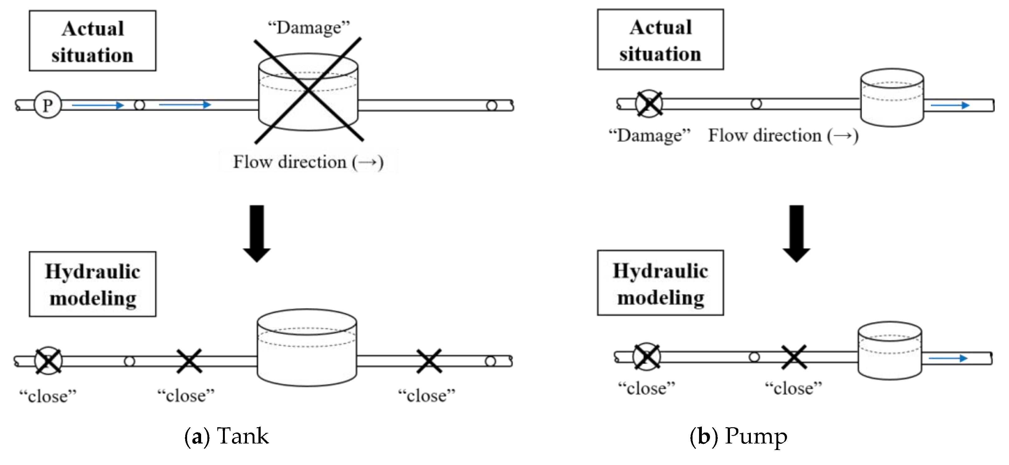
As shown in Figure 3, the model controls the front and rear pipelines directly connected to the damaged components to deactivate the water inflow and outflow to simulate the damaged tanks and pumps in EPANET. If a tank is damaged, the model closes the front and rear pipelines of the tank as described in Figure 3a. If a pump is connected to the failed tank, the pump operation is also suspended in the hydraulic simulation. If a pump failed, the status of the pump and discharge pipeline is set to “closed” so that there would be no active inflow to the downstream tank as illustrated in Figure 3b. Once the repair of the damaged tank or pump is completed, the closed pipelines and pumps would be set to “open” to simulate recovery of the facility.
(2) Hydraulic Simulation of Damaged Pipes
Water loss through a damaged pipe (broken or leaking) is a pressure-dependent flow expressed as Equation (7), which was proposed by Puchovsky [24]. In the model, the EPANET emitter option was utilized to calculate the water loss from the damaged pipes. Note the emitter option is assigned at a node in the EPANET simulation.
Here, Q = water loss through leaks/breaks; = discharge coefficient or emitter coefficient in EPANET (=, in which = gravitational acceleration, = specific weight of water, = opening area of the damaged pipe), and = operational pressure. Note the total opening area () of the leaks is assumed to be equivalent to 10% of the entire cross-sectional pipe area.
For the damaged pipelines, the discharge coefficient () is calculated first. If a pipe is considered to be broken, is assigned to the upper node of the flow direction. Then, the pipe status is set to “closed” and it does not function. Meanwhile, a pipe tagged as a leak may partially lose its function but still conveys water, and is assigned to the downstream node of the flow direction.
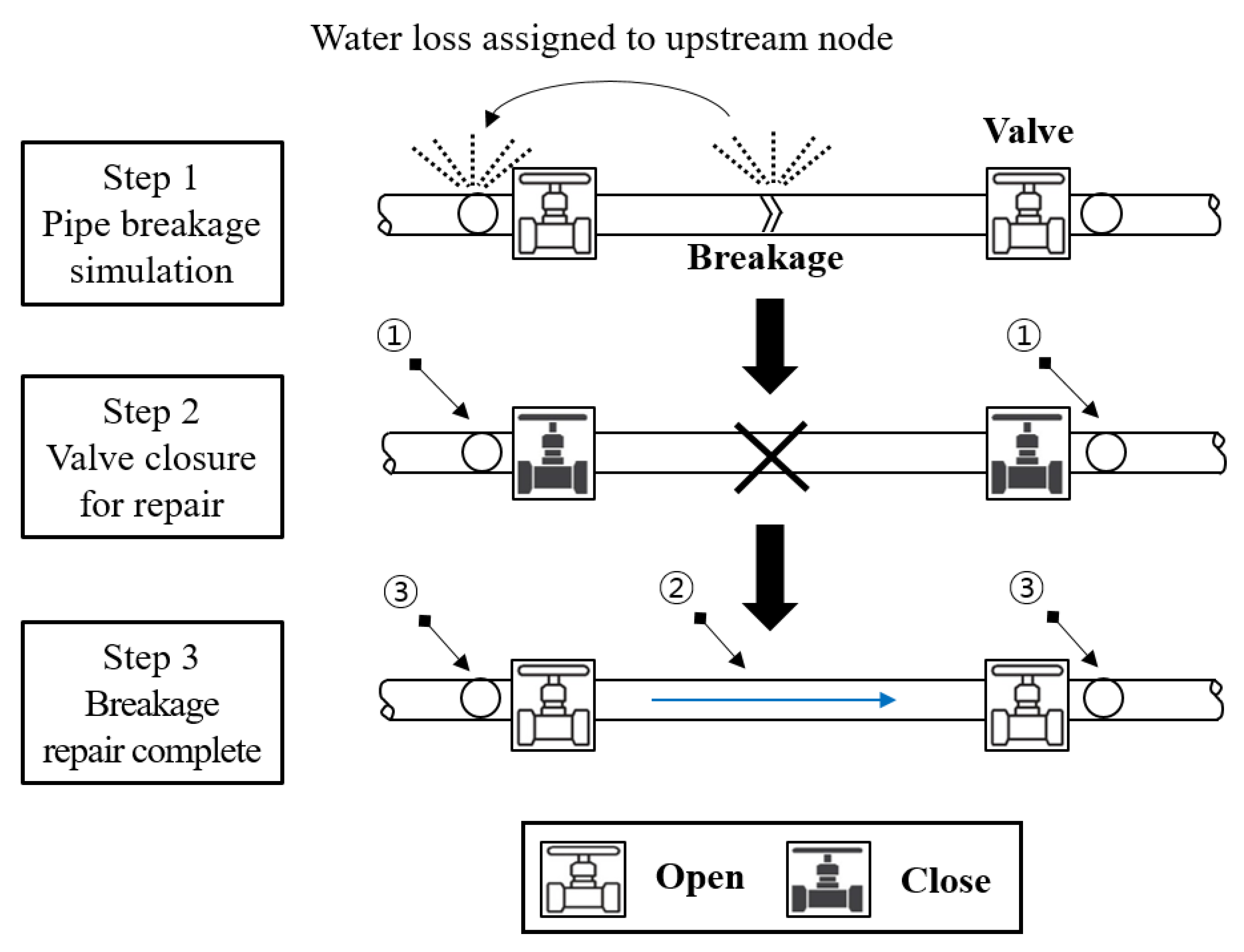
The repair of broken pipes begins after all the information related to damaged pipes is provided in the hydraulic analysis model (EPANET). Figure 4 illustrates the recovery steps of a broken pipe. Note that we assumed that shut-off valves exist at both ends of the damaged pipeline. Step 1 indicates that the water loss through the break is allocated to the upstream node for the hydraulic simulation. In step 2, the water loss through the broken pipe is stopped by closing the valves, and pipe repair begins. In the hydraulic simulation, the discharge coefficient () assigned at the upper node is set to zero to stop the water loss, and the pipe status is set to closed. After the pipe is isolated, the demand of nodes connected to the isolated pipe is modified to reflect water supply suspension during the pipe repair. In the model, the demands of both end nodes of the isolated pipe are reduced by the degrees of node (DoN), which is defined as the number of links that a node contains. As an example, the water supply to the upstream and downstream nodes are reduced by 50% respectively, since 1/DoN = 1/2 (①) as shown in Figure 4. In step 3, the pipe repair is completed, and the pipe status is set to “open” to enable water flow through the pipeline (②). Finally, the reduced water supply at the connected nodes recovers to the initial value (③).
2.2.3. Quantification of System Recovery
(1) Hydraulic Analysis under Pressure-Deficient Condition
The developed model used a quasi-PDA (quasi-pressure driven analysis) for hydraulic simulation of the seismic-damaged network in which a pressure-deficient condition may occur. The quasi-PDA treats the negative pressure by repeatedly performing DDA (demand driven analysis) and the procedure is briefly described as follows. First, given seismic-damaged condition, initial EPANET analysis (i.e., DDA) is performed. If negative pressures occur in the network, the base demands of the negative pressure nodes are set to zero (meaning that no water can be supplied to the nodes). DDA is then repeated. This process is repeated until no negative pressure appears in the network. A detail procedure of the quasi-PDA for the treatment of pressure-deficient condition is described in Yoo et al. [1].
(2) Calculation of System Serviceability
Once seismic damage occurs in a water network, the overall water supply capacity is degraded due to water losses through damaged pipes resulting in insufficient water pressure at demand nodes. To quantify system performance and recovery over time, an indicator called “system serviceability” was utilized. The system serviceability () represents the ability of a network to supply water and is calculated as the ratio of the actual supply to the required demand of the entire network. The system serviceability () can be used as an index to evaluate the water supply capacity of the system under a seismic damage and is calculated as shown in Equation (8) (Shi [25]; Wang [26]).
Here, = system serviceability index, = available (or serviceable) demand at node i, = required demand at node i, and N = total number of nodes.
The available nodal demand () is estimated based on the nodal pressure as expressed in Equation (9). If the water pressure at a node satisfies the minimum required pressure head (), then the required demand is fully supplied. If the water pressure at a node does not reach the minimum required pressure head (), the required demand is partially supplied depending on the nodal pressure. Lastly, no water can be supplied for a node with zero pressure.
Here, = nodal pressure at node i and = minimum required pressure head for full water supply.
(3) System Restoration Curve
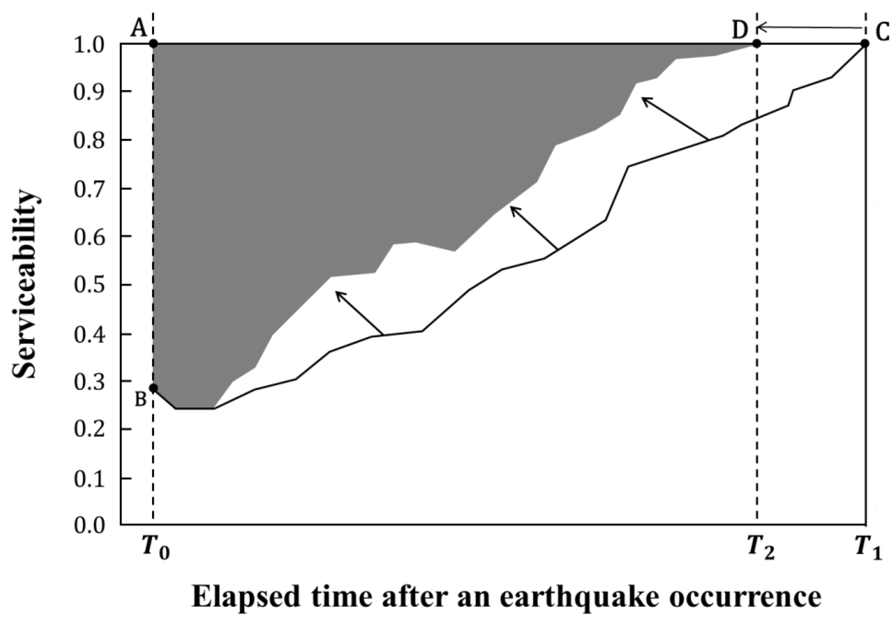
A system restoration curve is generated by estimating and plotting the system serviceability index over time as facility restoration proceeds as shown in Figure 5. Before an earthquake occurs, it is assumed that the system serviceability equals 1.0 (Point A) and the required water demand is fully supplied. An earthquake occurs at time , and the water serviceability drops to Point B. Subsequently, the water supply improves through restoration work, and the system state returns to normal at time (Point C). Let us call the restoration process following an [A → B → C] curve a basic strategy. If a more effective recovery approach is applied to the damaged network, the whole restoration curve might move from [A → B → C] to [A → B → D]. This implies that establishing an effective recovery strategy may help to reduce the restoration complete time ( → ) and also improve system serviceability during the restoration phase. The shaded area above the restoration curve in Figure 5 reflects both the depth and duration of the water supply shortage and is quantified in time (hours). Smaller curve areas indicate more effective restorations. Therefore, the serviceability index () and the area of the restoration curve can be utilized as indicators for quantitative comparison of different recovery strategies.
2.3. Summary of Assumptions and Simplifications
The assumptions used and simplifications made in the development and application of the model are summarized as follows. (1) All recovery personnel are available immediately after an earthquake and no shifts are considered. (2) The recovery equipment (crane, truck, etc.) and material usage (mechanical couplings, pipe sections, repair champs, etc.) were not considered in the simulation, only recovery personnel activity was simulated. (3) The application of the model is limited to the water pipe network; thus, interconnections with other lifeline networks (electric power, transportation, telecommunication, etc.) were not considered. (4) The transportation speed limit of the recovery personnel is set to 10 km/h by assuming that road conditions are not normal due to seismic damage. (5) The recovery simulation only considered the repairs of broken pipes. Locating and repairing the leaks will be more challenging and time-consuming compared to breaks and were excluded from the simulation. As a result, the system serviceability may not reach 100% even after the emergency repairs are completed due to water loss through unrepaired leaks. (6) Each pipeline has two shutoff valves at each end; thus, the pipe isolation for repair work only affects the customers connected to the isolated pipe.
3. Applications and Results
3.1. Application Network
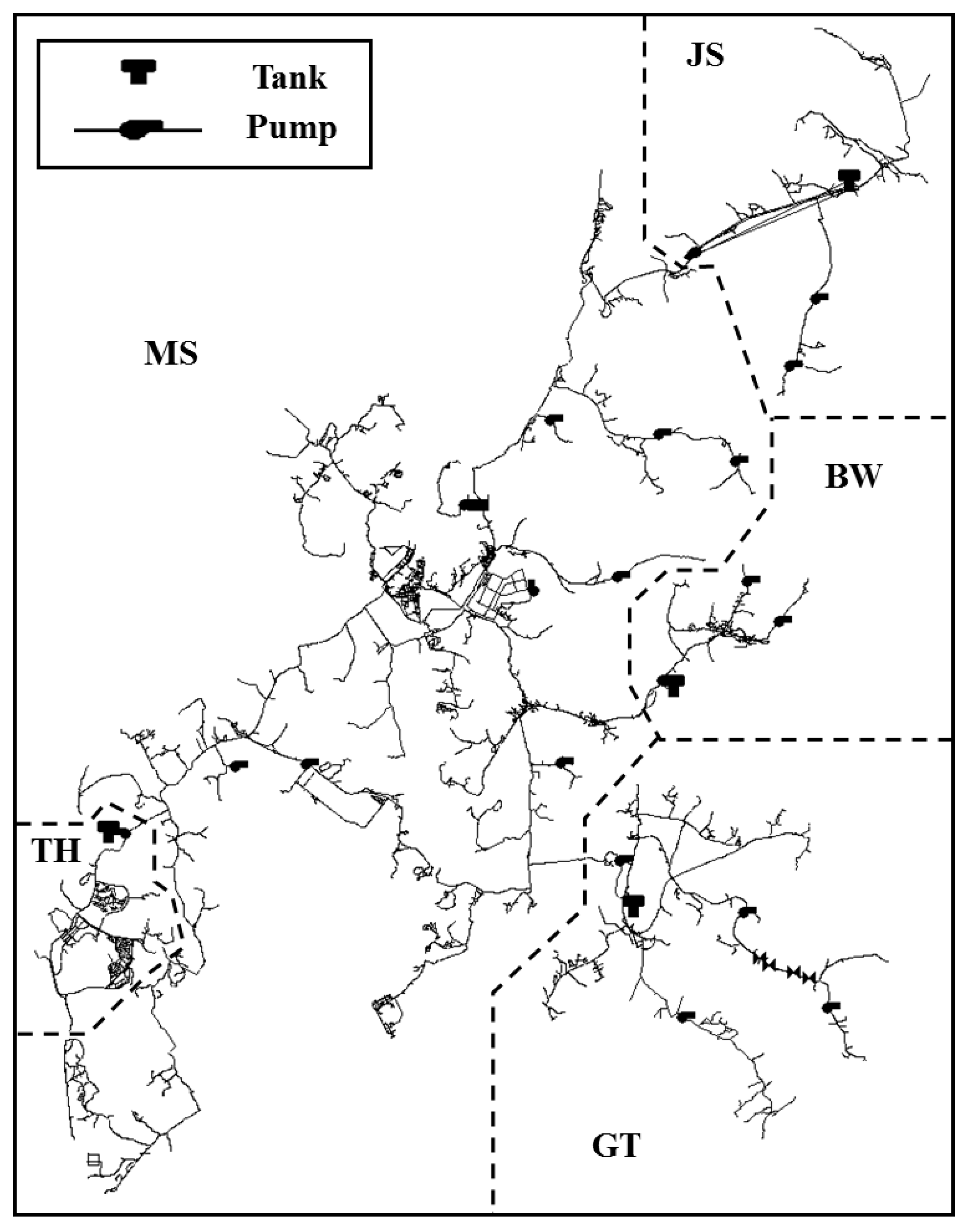
As a real-life demonstration, the developed model was applied to a P-city water supply network that is currently operating in South Korea (Figure 6). The study network consists of one water treatment plant (WTP), four ground tanks, four pumping stations, 8949 pipelines, 8381 nodes, and 18 in-line pumps. The diameter of the pipelines ranges from a minimum of 25 mm to a maximum of 1100 mm, and pipes with diameters of less than 100 mm account for 51.4% of the total system. The four large pumping stations lift water to the four high-elevation ground tanks, from which water is fed by gravity. The service area is primary residential and spans approximately 32 km by 34 km in west/east and north/south directions, respectively. It is composed of five administrative districts as seen in Figure 6. The MS area receives water directly from the WTP, while four other areas (JS, BW, GT and TH) are served from the ground storage tanks. Note that the total water demand is about 77,910 .
3.2. Recovery Scenarios
First, a virtual earthquake was simulated near the study area. The epicenter was located 16 km east of the network center with a depth of 10 km and an assumed magnitude of 5.0 (M5.0). The system restoration performance can vary greatly depending on the repair strategies. Here, diverse recovery rules were applied and evaluated using the model to deduce the most efficient recovery strategy applicable for the study network. The applied six recovery strategies (recovery priorities) are summarized in Table 1. First, the cases were mainly categorized depending on whether a network is divided into repair zones. The network zoning was applied to possibly shorten the repair team’s travel distance (the cases with the letter ‘B’). That is, the study network was grouped into five zones that correspond to the five administrative districts shown in Figure 6, and repair teams were deployed based on the repair zones. If the repair work is completed in a designated area, the repair team can travel to support other areas where the repair is still in progress. For cases without zoning (the cases with the letter ‘A’), all the repair teams would travel the entire network based on the repair priority without being allocated to a specific zone. Next, three specific recovery rules were suggested. Rule 1 states that the pipes delivering higher flows (generally those with a larger diameter) get the higher priority for repair. That is, the main transmission pipelines delivering higher flows, if damaged, will cause water suspension to a wide range of demand areas and need to be repaired first. Rule 2 indicates that the pipelines near water sources (WTP, ground tanks) should get priority. If the pipes near the water sources are damaged, there will be significant water loss in downstream areas, thus should be repaired first. Rule 3 suggests that the repair crews should move to the nearest repair location from the current repair-completed position, regardless of the flow rate or the distance from the sources. Rule 3 is likely to shorten the travel distance of the repair crews and consequently reduce the system recovery completion time. The recovery simulation was carried out hourly, the system restoration status was quantified, and the repair crew activity was recorded over time. For the study network, 50 repair personnel were available, and they were grouped into 10 teams (i.e., five personnel for each team). Note that for the cases with zoning (Cases B1~B3), two repair teams were allocated to each repair zone.
3.3. Simulation Results
3.3.1. Comparison of Restoration Strategies
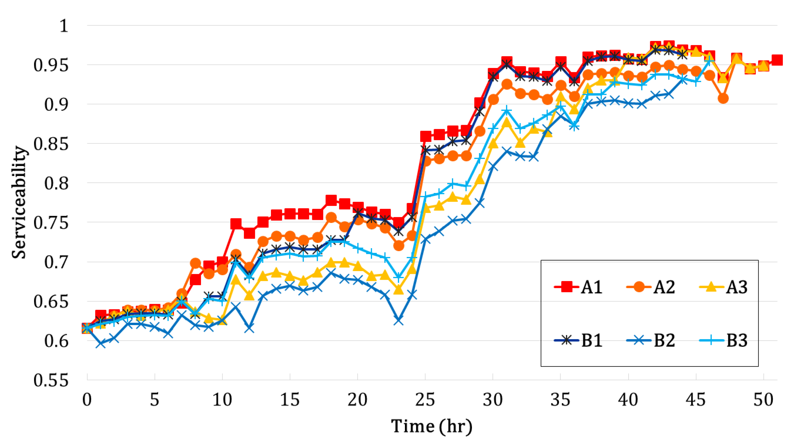
First, the restoration curves for each strategy were compared, as shown in Figure 7. Note the curves in general increase as the recovery progresses. However, at some time interval, the serviceability may decrease due to pipe isolation required for repair work. A sharp increase in serviceability was observed for all cases around 24–32 h of repair because the damaged tanks in BW, GT, TH areas were completely repaired around that time span. By resuming the water supply from the repaired ground tanks, the system serviceability increased significantly, indicating that the ground storage tanks play a significant role in the water supply of the studied network. We also observed that the system serviceability never reaches 100% since pipe leaks were not repaired. Note that the repair completion times are different for individual strategies. Comparing the six recovery scenarios, Case A1 seems the most efficient with the highest serviceability over time, while it takes the longest time to complete the repairs. Case A1 suggests that high flow pipes be repaired first regardless of the travel distance. Usually, when a main transmission line is damaged, the water supply is greatly affected. Thus, it is beneficial to repair such a pipeline first. The simulation results also reveal that network zoning is beneficial to reduce the repair completion time; that is, the repair completion times of B1~B3 are commonly shorter than those of A1~A3 as seen in Figure 7.
The system recovery curve allows intuitive and visual comparisons of the cases, but is not appropriate for quantitative comparisons. The curve area of each case was calculated for numerical comparisons. The curve area indicates the upper part of the restoration curve, and a smaller value denotes higher serviceability and shorter restoration times. The curve areas of each case are summarized in Table 2. Among the six applied cases, Case A1 showed the lowest curve area followed by Case B1. The results confirm that repairing the main pipelines first is advantageous in terms of restoration efficiency. Another important factor in evaluating the restoration strategy is to compare the recovery completion time, since delayed repairs may result in large socioeconomic losses. The total recovery time was measured as the time when the repairs of the broken pipes, damaged tanks and pumps were completed. Note the repair of pipe leaks was excluded in this study. As listed in Table 2, Case B1 was the quickest for completing the recovery. Overall, the cases with zoning (B1~B3) outperform the cases without zoning (A1~A3), showing a 15% reduction in total repair time.
Finally, it would be better to determine the most efficient restoration strategy by considering both the curve area and total repair time. A rank was assigned to each recovery strategy using the two evaluation criteria separately, and the results are summarized in Table 3. Case B1 was selected as the most efficient recovery strategy for the studied network (second best for curve area and the best for repair time). Therefore, in case of the study network, the most efficient restoration strategy was to dispatch the repair teams for each zone and primarily repair the main transmission lines.
3.3.2. Spatiotemporal Restoration Pattern
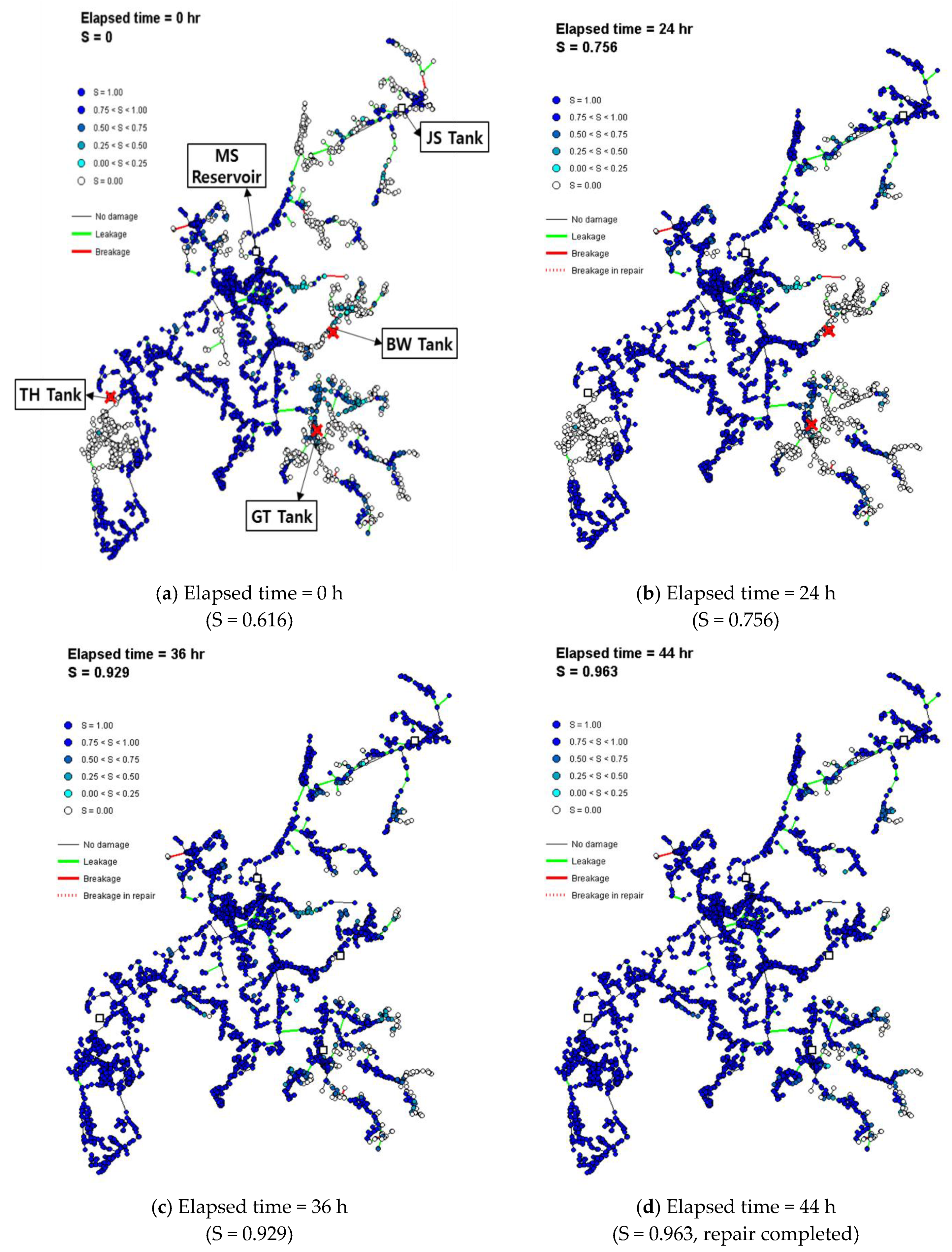
The restoration curve was used to understand the system-wide average recovery progress over time. In addition, it is required to monitor the spatial recovery conditions over the network as the restoration work progresses over time. Figure 8 shows the spatiotemporal distribution of system-wide serviceability illustrating the evolution of system restoration. Note that the system recovery simulation was performed by applying Case B1, which was determined to be the best recovery strategy in the previous analysis. Analyzing the snapshots, users can identify the locations of facility damage, the repairs in progress, and current conditions of water supply in an intuitive way. Figure 8a shows an initial damage state immediately after the earthquake. Among the four ground tanks, three (BW, GT, TH with ‘X’ mark) were damaged; thus, the downstream areas being supplied by the damaged tanks have significant effects of almost zero serviceability indicating no water to be supplied. Although the JS tank still operates without damage, the JS area is significantly damaged since the area is relatively close to the epicenter. After 24 h, TH tank was repaired, and the serviceability increased to 0.756, but two other tanks were still in repair (Figure 8b). After 36 h, all the damaged tanks were completely repaired, and the system recovered a function higher than 90% (Figure 8c). Finally, urgent repairs were completed after 44 h, and the serviceability reached 0.963 (Figure 8d). Note the system serviceability did not reach 100% because of unrepaired leaks throughout the network.
3.3.3. Repair Crew Activity
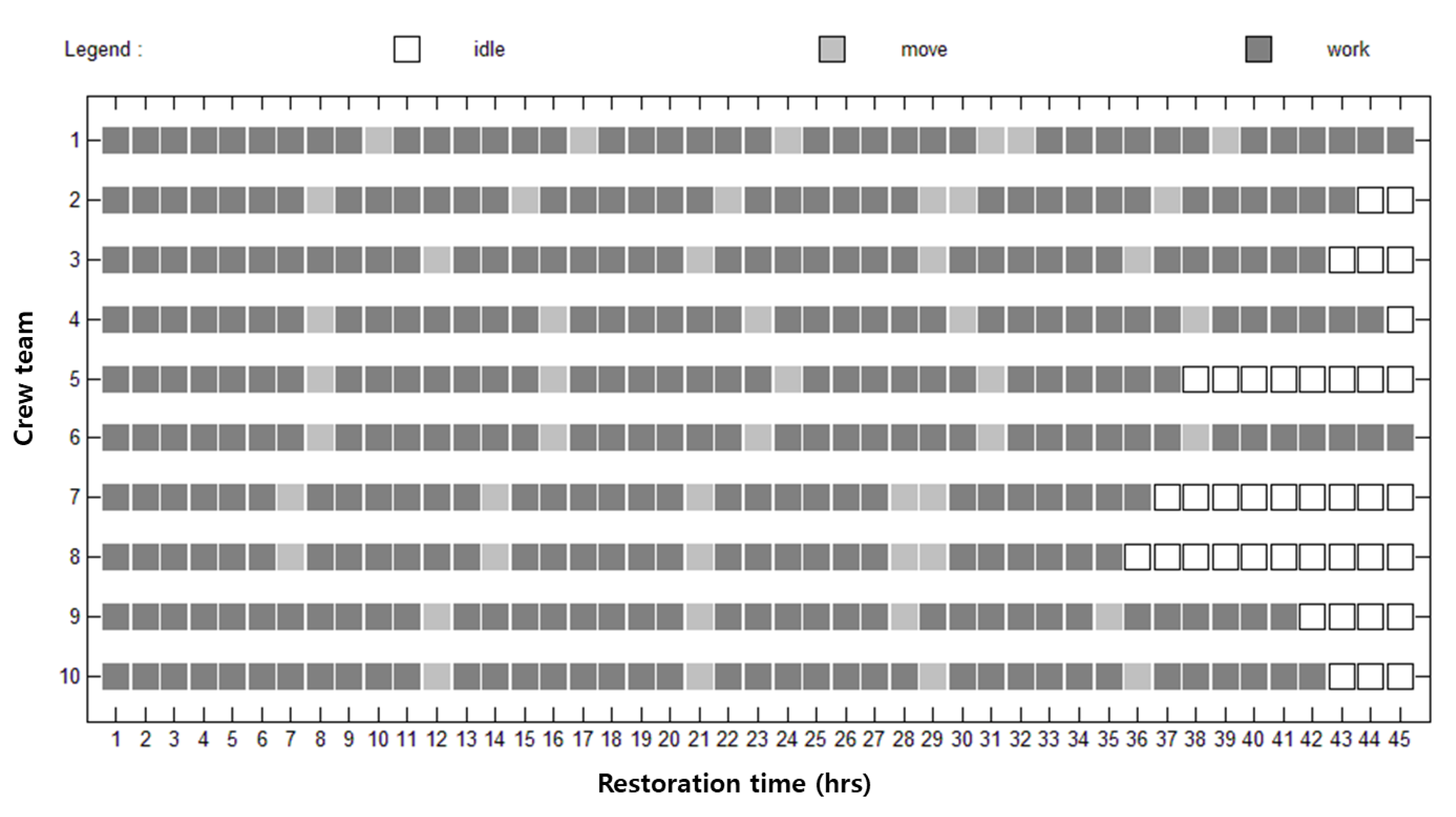
Estimating the repair team activity (including total number of repaired pipes, hourly work status, accumulated travel distance, and total working hours) would be helpful for both comparing recovery strategies and for estimating the required task force given seismic damage. Figure 9 illustrates the repair activities of individual teams over time when the restoration scenario of Case B1 was applied. Here, the “work” status means crew under repair, “move” indicates crew in travel, and “idle” implies the “on call” status because there is no remaining part to be repaired. The graph reveals that each team repaired approximately five to six pipes, and repairing a single damaged pipe took about six hours on average. We can also compare restoration strategies using the durations required for “work”, “move”, and “idle” status. Table 4 compares the average working, moving, and waiting hours of ten repair teams for the applied six restoration cases. Overall, we found that the restoration cases with zoning (B1~B3) required fewer hours for repair and travel compared to the cases without zoning (A1~A3). That is, on average 7 h (5 h for repair and 2 h for travel) were saved by district-based repairs. Note that the waiting hours were similar for both case groups. Using this statistical analysis of the repair crew activities, the work intensity of each team can be estimated, the restoration strategies can be assessed, and finally repair crews can be assigned in a more efficient way.
3.3.4. Impact on Tank Water Level
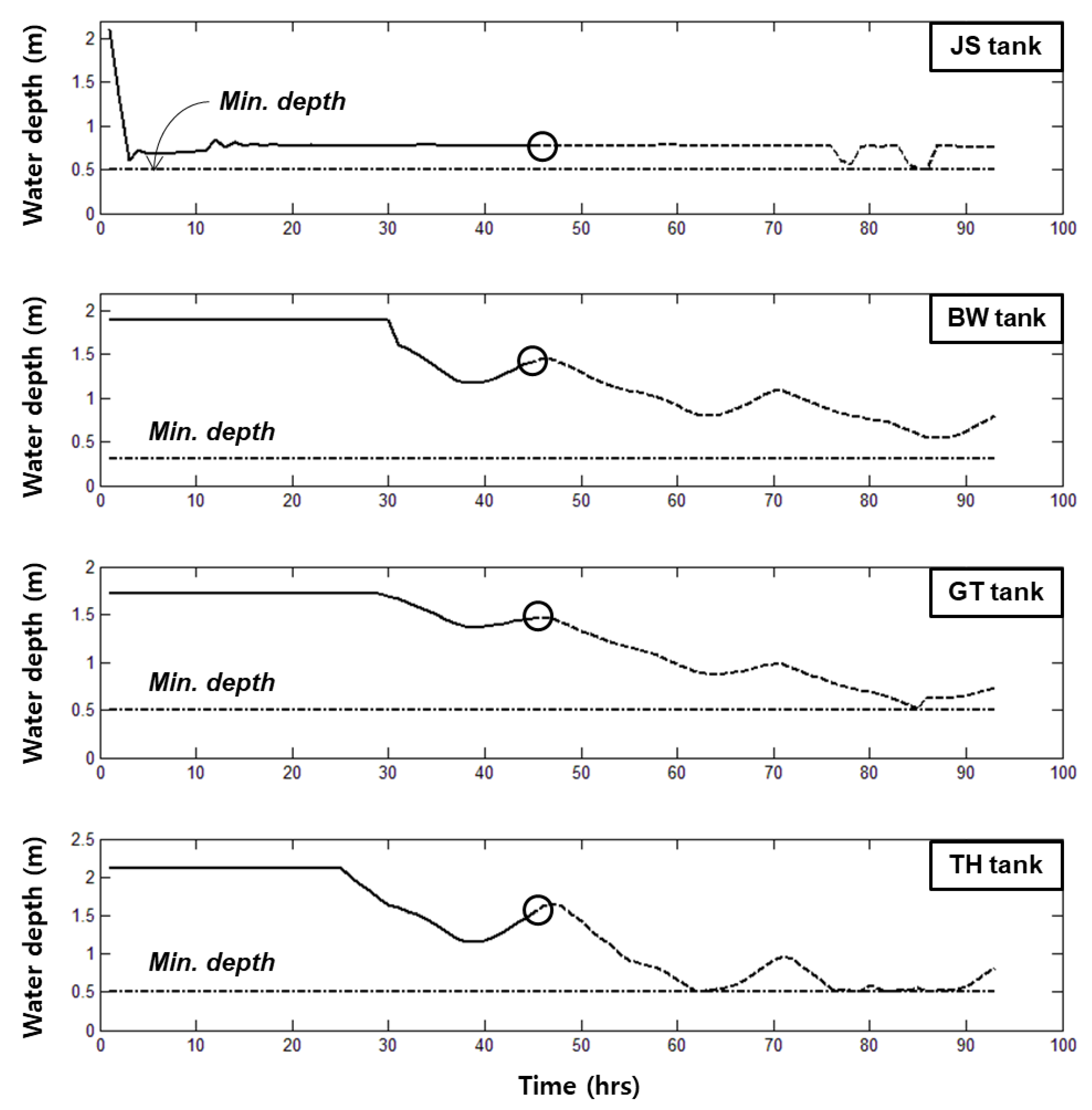
A ground storage tank stores and distributes a large amount of water. Thus, it plays a significant role in a water distribution system. When a WTP cannot supply water temporarily due to an emergency (e.g., power outage, pump failure, etc.), the storage tank can supply downstream service area for a certain period to mitigate the damage. Figure 10 illustrates the fluctuations of tank water level after an earthquake. Here, the solid line indicates the water level while the repair was in progress and the dotted line implies the tank water level after the emergency repair was completed (48 h later, approximately). Note the JS tank continued the service without the seismic damage, while other three tanks were damaged (operation ceased for repair) and recovered. The water level of the damaged tank is set to its initial value assuming no inflow and outflow from the tank until the repair is completed. It is observed that the tank water level declines and reaches a minimum operational depth even after the emergency repair has been completed. This is because of additional water loss through the unrepaired pipe leaks over the network. Therefore, to return to its normal operating condition, prompt leakage detection and repair would be required throughout the network.
4. Conclusions
A computer-based simulation model was developed for the post-earthquake restoration simulation of water supply networks. The main purpose of the model was to derive a system-specific recovery strategy to enhance the resilience of the damaged network in terms of post-earthquake restoration. The model can reflect various seismic damage scenarios (epicenter location and seismic magnitude) to determine the potential damage to facilities. Given damage conditions (either from the simulation or collected information from the field), the model determines the appropriate recovery schemes, including the repair sequence rule and crew allocation decisions. Once the system recovery starts based on the user defined rules, the model provides the recovery progress information, such as the required repair completion time, required recovery resources, spatiotemporal restoration progress, and repair crew activity information for analysis. Using the information, the model can serve as a decision support tool for rapid and efficient system remedy.
The proposed model was applied to a P-city water supply network currently operating in South Korea as a real-life demonstration. It was possible to obtain the most effective scheme to recover the damaged network by applying six potential restoration strategies. We utilized the system serviceability index and the restoration curve to quantitatively evaluate the applied restoration strategy and intuitively assess the recovery process. The application results revealed that the most effective restoration strategy for the study network was ‘Case B1’, which separately dispatch the repair teams based on the pre-assigned repair zones and primarily repair the main transmission lines that deliver higher flows. The post-simulation analyses included further analysis of the spatiotemporal distribution of serviceability in graphical form, in which users can identify the locations of facility damage, repairs in progress, and current conditions of water supply. In addition, the statistical analysis of the repair crew activities revealed the work intensity of each repair team, from which system managers can determine alternative resources dispatch plans. The proposed model depicts a real-life process, thus can be used by system operators, engineers, and decision makers to better serve their community in an urgent situation.
Since the seismic damage is unpredictable and hard to simulate, the model results may have limited accuracy. To advance the developed model, we are planning to resolve the assumptions and simplifications embedded in the current model. First, the actual travel route of repair crews should be estimated based on the road network in conjunction with the water network for more accurate estimates of the required travel distance. For an interconnected simulation, it would be better to utilize a geographic information system (GIS) for both water-pipe and road networks. Second, the shut-off valve locations should be considered to identify the actual suspended area (depicted by a segment) while the pipe repairs are undertaken. Third, a full-PDA solver should be coupled with the model for accurate hydraulic analysis of pressure-deficient conditions. These are fruitful and encouraging topics to pursue in the future to advance the current model.
Author Contributions
J.C. carried out the analysis of proposed method, model simulations and drafted the manuscript. D.G.Y. surveyed the previous studies and provided conceptual ideas of the proposed model. D.K. conceived the original idea of the study and finalized the manuscript.
Funding
This research was supported by (1) Basic Science Research Program through the National Research Foundation of Korea (NRF) funded by the Ministry of Education, Science and Technology (NRF-2016R1A2B4014273) and (2) Korea Agency for Infrastructure Technology Advancement (KAIA) grant funded by the Ministry of Land, Infrastructure and Transport (Grant 18AWMP-B083066-05).
Conflicts of Interest
The authors declare no conflicts of interest.
References
- Yoo, D.G.; Jung, D.; Kang, D.; Kim, J.H.; Lansey, K. Seismic hazard assessment model for urban water supply networks. J. Water Resour. Plan. Manag. 2015, 142, 04015055. [Google Scholar] [CrossRef]
- Yoo, D.G.; Kang, D.; Kim, J.H. Optimal design of water supply networks for enhancing seismic reliability. Reliab. Eng. Syst. Saf. 2016, 146, 79–88. [Google Scholar] [CrossRef]
- Federal Emergency Management Agency (FEMA). HAZUS97 Technical Manual; FEMA: Washington, DC, USA, 1997. [Google Scholar]
- Mid America Earthquake (MAE) Center. MAEviz Software. Available online: http://mae.cee.illinois.edu/software/software_maeviz.html (accessed on 10 October 2018).
- Shi, P.; O’Rourke, T.D.; Wang, Y. Simulation of earthquake water supply performance. In Proceedings of the 8th National Conf. on Earthquake Engineering, San Francisco, CA, USA, 18–22 April 2006. [Google Scholar]
- Yoo, D. Seismic Reliability Assessment for Water Supply Networks. Ph.D. Thesis, Korea University, Seoul, Korea, 2018. [Google Scholar]
- Adachi, T.; Ellingwood, B.R. Serviceability of earthquake-damaged water systems: Effects of electrical power availability and power backup systems on system vulnerability. Reliab. Eng. Syst. Saf. 2008, 93, 78–88. [Google Scholar] [CrossRef]
- Yoo, D.G.; Jung, D.; Kang, D.; Kim, J.H.; Lansey, K. Seismic Reliability–Based Multiobjective Design of Water Distribution System: Sensitivity Analysis. J. Water Resour. Plan. Manag. 2016, 143, 06016005. [Google Scholar] [CrossRef]
- Davenport, P.N.; Lukovic, B.; Cousins, W.J. Restoration of earthquake damaged water distribution systems, in “Remembering Napier 1931”. Paper No. 44. In Proceedings of the 2006 Conference of the New Zealand Society for Earthquake Engineering, Napier, New Zealand, 10–12 March 2006. [Google Scholar]
- Tabucchi, T.; Davidson, R.; Brink, S. Restoring the Los Angeles water supply system following an earthquake. In Proceedings of the 14th World Conference on Earthquake Engineering, Beijing, China, 12–17 October 2008. [Google Scholar]
- Luna, R.; Balakrishnan, N.; Dagli, C.H. Poste-arthquake recovery of a water distribution system: Discrete event simulation using colored petri nets. J. Infrastr. Syst. 2011, 17, 25–34. [Google Scholar] [CrossRef]
- Tabucchi, T.; Davidson, R.; Brink, S. Simulation of post-earthquake water supply system restoration. Civ. Eng. Environ. Syst. 2010, 27, 263–279. [Google Scholar] [CrossRef]
- Davis, C.A.; O’Rourke, T.D.; Adams, M.L.; Rho, M.A. Case study: Los Angeles water services restoration following the 1994 Northridge earthquake. In Proceedings of the 15th World Conference on Earthquake Engineering, Lisbon, Portugal, 24–28 September 2012. [Google Scholar]
- Davis, C.A. Water system service categories, post-earthquake interaction, and restoration strategies. Earthq. Spectra 2014, 30, 1487–1509. [Google Scholar] [CrossRef]
- Davis, C.A.; Giovinazzi, S. Toward Seismic Resilient Horizontal Infrastructure Networks. In Proceedings of the 6th International Conference on Earthquake Geotechnical Engineering, Christchurch, New Zealand, 2–4 November 2015. [Google Scholar]
- Klise, K.A.; Hart, D.; Moriarty, D.; Bynum, M.L.; Murray, R.; Burkhardt, J.; Haxton, T. Water Network Tool for Resilience (WNTR) User Manual; EPA/600/R-17/264; U.S. Environmental Protection Agency: Washington, DC, USA, 2017. Available online: https://cfpub.epa.gov/si/si_public_record_report.cfm?dirEntryId=337793 (accessed on 6 June 2017).
- Klise, K.A.; Bynum, M.; Moriarty, D.; Murray, R. A software framework for assessing the resilience of drinking water systems to disasters with an example earthquake case study. Environ. Modell. Softw. 2017, 95, 420–431. [Google Scholar] [CrossRef]
- MATLAB User’s Manual; The MathWorks, Inc.: Natick, MA, USA, 2000.
- Rossman, L.A. EPANET 2: Users Manual; U.S. Environmental Protection Agency (EPA): Cincinnati, OH, USA, 2000.
- Baag, C.E.; Chang, S.J.; Jo, N.D.; Shin, J.S. Evaluation of seismic hazard in the southern part of Korea. In Proceedings of the 2nd International Symposium on Seismic Hazards and Ground Motion in the Region of Moderate Seismicity, Seoul, Korea, 1 November 1998; pp. 31–50. [Google Scholar]
- Eidinger, J. Seismic Fragility Formulations for Water Systems; American Lifelines Alliance, G&E Engineering Systems Inc.: Olympic Valley, CA, USA, 2001. [Google Scholar]
- Isoyama, R.; Ishida, E.; Yune, K.; Shirozu, T. Seismic damage estimation procedure for water supply pipelines. Water Supply 2000, 18, 63–68. [Google Scholar]
- Chang, Y.-H.; Kim, J.-H.; Jung, K.-S. A Study on the design and evaluation of connection pipes for stable water supply. J. Korean Soc. Water Wastewater 2012, 26, 249–256. [Google Scholar] [CrossRef] [Green Version]
- Puchovsky, M.T. (Ed.) Automatic Sprinkler Systems handbook; National Fire Protection Association (NFPA): Quincy, MA, USA, 1999. [Google Scholar]
- Shi, P.; O’Rourke, T.D. Seismic Response Modeling of Water Supply Systems; MCEER: Buffalo, NY, USA, 2006. [Google Scholar]
- Wang, Y.; O’Rourke, T.D. Seismic Performance Evaluation of Water Supply Systems; MCEER: Buffalo, NY, USA, 2006. [Google Scholar]
Figure 1.
Model simulation flow chart.

Figure 2.
Fragility curves for tank (top) and pump (bottom) (data from ALA, 2001 [21]).
Figure 2.
Fragility curves for tank (top) and pump (bottom) (data from ALA, 2001 [21]).

Figure 3.
Hydraulic modeling of damaged tanks and pumps.

Figure 4.
Pipe breakage repair simulation steps.

Figure 5.
System restoration curve.

Figure 6.
P-city water supply network layout.

Figure 7.
System restoration curves of six recovery strategies.

Figure 8.
Spatiotemporal distribution of system serviceability over time.

Figure 9.
Repair crew activity chart.

Figure 10.
Tank water level fluctuation.


Table 1.
System restoration strategies.
| Case | Zoning | Rule | Description |
|---|---|---|---|
| A1 | No | 1 | Pipes carrying higher water flow get higher repair priority |
| A2 | No | 2 | Pipes closer to water sources get higher repair priority |
| A3 | No | 3 | Pipes nearest to a current repair point get priority |
| B1 | Yes | 1 | Pipes carrying higher water flow get higher priority within a zone |
| B2 | Yes | 2 | Pipes closer to water sources get higher priority within a zone |
| B3 | Yes | 3 | Pipes nearest to a current repair point get priority within a zone |
Table 2.
Restoration curve area and repair completion time.
| Case | Curve Area (h) | Completion Time (h) |
|---|---|---|
| A1 | 8.9 | 53 |
| A2 | 9.8 | 52 |
| A3 | 11.1 | 53 |
| B1 | 9.3 | 45 |
| B2 | 12.0 | 46 |
| B3 | 10.7 | 48 |
Table 3.
Restoration total rank.
| Case | Rank for Curve Area | Rank for Repair Time | Total Rank Sum |
|---|---|---|---|
| A1 | 1 | 5 | 6 |
| A2 | 3 | 4 | 7 |
| A3 | 5 | 5 | 10 |
| B1 | 2 | 1 | 3 |
| B2 | 6 | 2 | 8 |
| B3 | 4 | 3 | 7 |
| Best case/Total rank sum | Case B1/3 | ||
Table 4.
Average repair crew activity information for different recovery strategies.
| Case | Average Time for Repair (h) | Average Time for Travel (h) | Average Time for Wait (h) |
|---|---|---|---|
| A1 | 41.3 | 7.7 | 4.0 |
| A2 | 41.3 | 6.5 | 5.1 |
| A3 | 41.4 | 7.1 | 4.5 |
| B1 | 36.2 | 4.8 | 4.0 |
| B2 | 36.2 | 5.2 | 4.6 |
| B3 | 37.0 | 5.3 | 5.7 |
© 2018 by the authors. Licensee MDPI, Basel, Switzerland. This article is an open access article distributed under the terms and conditions of the Creative Commons Attribution (CC BY) license (http://creativecommons.org/licenses/by/4.0/).
Share and Cite
MDPI and ACS Style
Choi, J.; Yoo, D.G.; Kang, D. Post-Earthquake Restoration Simulation Model for Water Supply Networks. Sustainability 2018, 10, 3618. https://0-doi-org.brum.beds.ac.uk/10.3390/su10103618
AMA Style
Choi J, Yoo DG, Kang D. Post-Earthquake Restoration Simulation Model for Water Supply Networks. Sustainability. 2018; 10(10):3618. https://0-doi-org.brum.beds.ac.uk/10.3390/su10103618
Chicago/Turabian StyleChoi, Jeongwook, Do Guen Yoo, and Doosun Kang. 2018. "Post-Earthquake Restoration Simulation Model for Water Supply Networks" Sustainability 10, no. 10: 3618. https://0-doi-org.brum.beds.ac.uk/10.3390/su10103618
Note that from the first issue of 2016, this journal uses article numbers instead of page numbers. See further details here.