A Hybrid Wind Speed Forecasting Method and Wind Energy Resource Analysis Based on a Swarm Intelligence Optimization Algorithm and an Artificial Intelligence Model

Abstract

Wind power has the most potential for clean and renewable energy development. Wind power not only effectively solves the problem of energy shortages, but also reduces air pollution. In recent years, wind speed time series analyses have increasingly become a concern of administrators and power grid dispatchers searching for a reasonable way to reduce the operating cost of wind farms. However, analyzing wind speed in detail has become a difficult task, because the traditional models sometimes fail to capture data features due to the randomness and intermittency of wind speed. In order to analyze wind speed series in detail, in this paper, an effective and practical analysis system is studied and developed, which includes a data analysis module, a data preprocessing module, a parameter optimization module, and a wind speed forecasting module. Numerical results show that the wind time series analysis system can not only assess wind energy resources of a wind farm, but also master future changes of wind speed, and can be an effective tool for wind farm management and decision-making.

1. Introduction

Wind power makes use of air flow through wind turbines to mechanically power generators for electric power. The total global installed capacity reached 487 GW by the end of 2016, and new installed capacity was more than 54.6 GW in 2016, of which 23.4 GW of new installations in China powered this growth in large part [1]. The rapid increase of global installation capacity means that one of the largest onshore wind farms, Gansu Wind Farm [2], which has installed capacity of over 6000 MW, has already started operation. In order to ensure reliability and safe operation, detailed analysis of the situation of large wind farms is an important task for wind farm management and decision-making.

Assessing wind energy resources involves analyzing and evaluating the long-term wind energy reserves of wind farms [3]. Through detailed assessment of the time series of a wind farm, some characteristics of wind energy are calculated, such as average wind speed, average wind power density, effective wind power density, and available hours. The probability statistics method uses a variety of distribution functions (such as Rayleigh distribution, gamma distribution, logistic distribution, and Weibull distribution [4]) to fit the probability distribution of wind speed and find the optimal probability distribution function. When the optimal probability distribution function is found, its parameters need to be estimated by a numerical method or optimization algorithm. For example, Mohammadi et al. [5] used multinumerical methods to evaluate the parameters of the Weibull distribution. Wu et al. [6] compared three probably density functions and selected the best one to apply the wind energy assessment. For the optimization parameters, three particle swarm optimization algorithms and 18 differential evolution algorithms were used to estimate the parameters of the Weibull distribution.

However, numerical estimation methods such as moments estimate [7], maximum likelihood estimate [8], and least squares estimate [9], have some disadvantages and restricted conditions. For example, the method of moment can only be used in the distribution when the population origin moment exists and the moment only has some of the information, and this method only has good performance when the sample size is large. The maximum likelihood estimation must incorporate the sample distribution. It is more complicated to incorporate the likelihood equations, which often obtain the approximate solution by computer iterative computation. However, the least squares method has two kinds of defects. If the noise of the model is colored noise, the estimation result of the least squares is a biased estimation; with increasing data size, “data saturation” will appear.

Due to the defects of the above methods, in this paper, four optimization algorithms (firefly algorithm [10], genetic algorithm [11], ant colony algorithm [12], and cuckoo search algorithm [13]) are used to optimize and determine the shape (k) and scale (c) parameters of the Weibull distribution function for calculating wind power density.

The wind energy assessment is used to analyze long-term wind energy reserves and calculate long-term electricity production. However, the wind energy assessment is not comprehensive in the detailed analysis of wind farms. At same time, it is important to master future changes of wind speed. Over the past few decades, many researchers have proposed methods of wind speed forecasting. For example, Cassola et al. [14] improved the forecasting performance of wind speed by using a Kalman filtering technique to correct the numerical weather prediction model output. Liu et al. [15] proposed two hybrid models based on Auto-Regressive and Moving Average Model (ARMA) and nonparametric models, and showed that nonparametric-based hybrid models generally outperformed the other models. Tascikaraoglu et al. [16] proposed a novel wind speed prediction model using wavelet transform and spatiotemporal methods, which improved the short-term wind speed forecasting relative to other benchmark models. Xiao et al. [17] developed a hybrid wavelet neural network (WNN) model with an improved cuckoo search algorithm. The above studies used four classes to forecast wind speed: physical model, conventional statistical model, spatial correlation model, and artificial intelligence model.

However, traditional forecasting methods have some defects. For example, the physical methods require considerable observed data with limited simulation scale and consume a lot of computing resources, which are expensive to obtain [18]. On the other hand, these methods are more suitable for weather forecasting instead of wind speed forecasting [19]. Statistical models cannot address forecasting with high noise and fluctuation, irregular nonlinear trends, or features of wind speed series data, which is mainly limited by the prior assumption of linear form among time series. The spatial correlation model [20] makes it quite difficult to implement perfect wind speed forecasting due to the vast quantities of information that need to be considered and collected, such as wind speed values of many spatially correlated sites. There are still many disadvantages and defects with artificial intelligence methods, for example, easily getting into local optimum, overfitting, and exhibiting a relatively low convergence rate [21].

In view of the disadvantages of wind energy resource assessment and traditional forecasting models, in this paper, a wind energy analysis system that includes an assessment module and a forecasting module is developed. The system can be an effective estimation and forecasting tool for large wind farms.

The major contributions of this paper are as follows:

(1)

A wind energy analysis system including an assessment of wind energy resources and forecasting of wind speed time series, is developed and applied. The purpose of the wind energy assessment is to analyze the wind energy reserves of the wind farm, and the purpose of wind speed forecasting is to master the future changes of wind speed.

(2)

To effectively assess wind energy, the performance of different probability density functions (PDFs) is compared so as to select the best one. As one of the most suitable probability distributions, the probability density function is the most applicable approach to describe the distribution of wind speed in this case.

(3)

When the parameters of the probability density function are determined, in place of the numerical estimation method, which has some defects for estimation parameters, the optimization algorithm can effectively obtain optimal parameters.

(4)

Because actual wind speed has chaotic noise, which will decrease the accuracy of the forecasting, data preprocessing technology is employed to reduce noise and uncertainty of wind speed series.

(5)

A wind speed forecasting module, which includes a data preprocessing module, parameter optimization module, and forecasting module, is developed. In order to determine the parameters of the least squares support vector machine (LSSVM), a hybrid optimization algorithm is proposed. The new optimization algorithm uses the steepest descent to improve the convergence rate of the cuckoo search algorithm, which can effectively improve the forecasting accuracy of the LSSVM.

2. Model Construction

This part mainly introduces the composition of the hybrid algorithm and the detailed steps. Step one: introduce correlation algorithm for wind speed data analysis. Step two: actual wind speed data is processed by wavelet packet transform, which is used to establish the LSSVM. Then the modified cuckoo search algorithm is used to optimize the parameters of the LSSVM.

2.1. The Correlation Algorithm for Wind Speed Data Analysis

At a wind farm, the air density and natural terrain environment are constant, which has less influence on wind energy resources. Only the wind speed will change with the movement of the atmosphere. Thus, the frequency distribution of wind speed can measure the distribution of wind energy resources at the wind farm. In this paper, four kinds of probability distribution are used to fit the wind density [22].

Table 1. The different kinds of probability density function.

Probability Distribution	Probability Density Function
Gamma distribution	y = f$(x|a,b)=\frac{1}{b^a\mathrm{\Gamma }(a)}{x}^{a-1}{e}^{\frac{-x}{b}}$ where $\mathrm{\Gamma }(\cdot )$ is Gamma function
Normal distribution	y = f(x|μ, σ) = $\frac{1}{\sigma \sqrt{2\pi }}\exp (\frac{{-(x-\mu )}^2}{{2\sigma }^2})$
Rayleigh distribution	y = f(x|b) = $\frac{x}{b^2}\exp (\frac{{-x}^2}{{2b}^2})$
Weibull distribution	y = f(x|a, b) = $\frac{b}{a}{(\frac{x}{a})}^{b-1}\exp (-{\left(\frac{x}{a}\right)}^b)$

shows the different probability density functions.

In order to determine the parameters of the probability density functions, in this paper, four kinds of optimization algorithm are employed: differential evolution algorithm [23], particle swarm optimization algorithm [24], cuckoo search algorithm [23], and genetic algorithm [22].

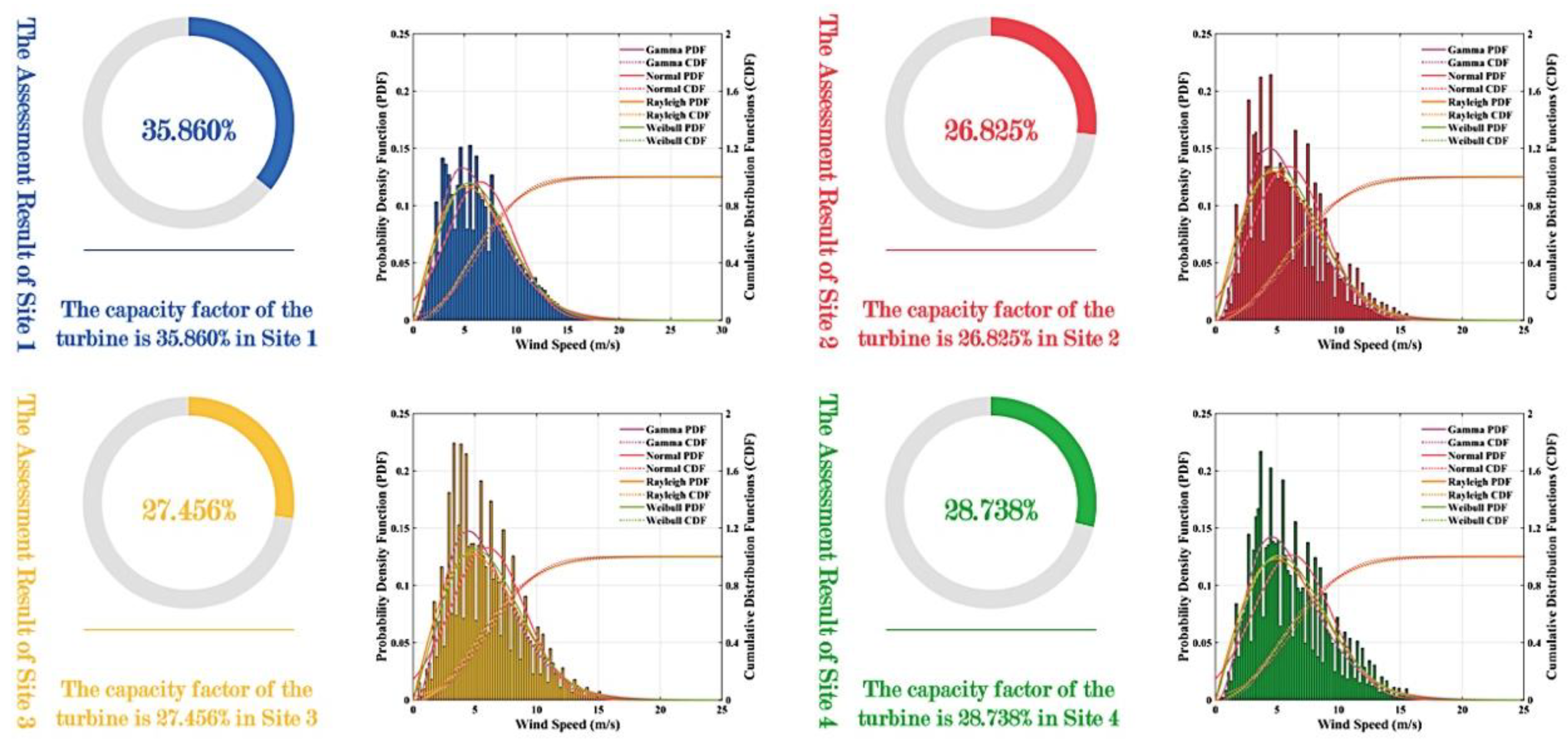
The performance of a wind turbine installed at a given site can be examined by the amount of mean power output over a period of time (Pout) and the conversion efficiency or capacity factor [23] of the turbine. The mean power output Pout can be calculated using the following expression based on the Weibull distribution function:

$$C_f=\frac{e^{-(\frac{V_c}{c}{)}^k}{-e}^{-(\frac{V_r}{c}{)}^k}}{{(\frac{V_r}{c})}^k-(\frac{V_c}{c}{)}^k}{-e}^{-(\frac{V_f}{c}{)}^k}$$

(1)

where v_c, v_r, v_f are the cut-in wind speed, rated wind speed, and cut-off wind speed, respectively. It should be mentioned that the above expressions are only valid for the assessment of wind turbines.

2.2. The Method of Data Pre-Processing: Wavelet Packet Transform

In the wavelet packet framework, compression and denoising ideas are exactly the same as those developed in the wavelet framework. The only difference is that wavelet packets [24] offer a more complex and flexible analysis, because in wavelet packet analysis, the details as well as the approximations are split.

A single wavelet packet decomposition gives a lot of bases from which to look for the best representation with respect to a design objective. This can be done by finding the “best tree” based on an entropy criterion.

Denoising and compression are interesting applications of wavelet packet analysis. The wavelet packet denoising or compression procedure involves four steps:

Step 1:

Decomposition. For a given wavelet, compute the wavelet packet decomposition of signal x at level N.

Step 2:

Computation of the best tree. For a given entropy, compute the optimal wavelet packet tree. Of course, this step is optional. The graphical tools provide a “Best Tree” button to make this computation quick and easy.

Step 3:

Thresholding of wavelet packet coefficients. For each packet (except for the approximation), select a threshold and apply thresholding to coefficients.

The graphical tools automatically provide an initial threshold based on balancing the amount of compression and retained energy. This threshold is a reasonable first approximation for most cases. However, in general, you will have to refine your threshold by trial and error so as to optimize the results to fit your particular analysis and design criteria.

The tools facilitate experimentation with different thresholds and make it easy to alter the trade-off between the amount of compression and retained signal energy.

Step 4:

Reconstruction. Compute wavelet packet reconstruction based on the original approximation coefficients at level N and the modified coefficients.

2.3. L.SSVM (Least Square Support Vector Machine)

Least squares support vector machine, proposed by Suyken et al. [25], is an improved support vector machine, and is one of the important results of statistical learning theory in recent years. Compared with the traditional method of SVM, LSSVM has the following advantages: (1) equality constraints replace the inequality constraints in the traditional SVM algorithm; and (2) solving the quadratic program is changed into solving the linear equations directly.

The least squares support vector machine algorithm is described as follows:

For a given training set (p_i, q_i), where i = 1,2,3,⋯,n, $p_i\in R^n$, $q_i\in R$, LSSVM uses a nonlinear mapping ϕ(p) to map samples from the original space Rⁿ to the feature space, and ϕ(p_i) to construct the optimal decision function in high-dimensional feature space:

p(q) = ω·ϕ(p) + b

(2)

Therefore, the nonlinear estimation function is transformed into a linear high-dimensional feature space estimation function, and looking for ω, b is minimized through the structural risk minimization principle:

$$R=\frac{1}{2}\Vert \omega {\Vert }^2+C\cdot R_{emp}$$

(3)

In Equation (3), $\Vert \omega {\Vert }^2$ controls the complexity of the model; C is the regularization parameter that controls the severity of the error samples; and R_emp is the error control function that is an insensitive loss function of ε. The frequently used loss functions are linear ε loss function, quadratic ε loss function, and Huberg loss function. Different forms of support vector machine can be constructed by selecting different loss functions. According to the structural risk minimization principle, a regression problem is expressed as a constrained optimization problem:

$$\min J(\omega ,\zeta )=\frac{1}{2}\omega \cdot \omega +C{{\displaystyle \sum }}_{i=1}^n{\zeta }_i^2(\mathrm{s}.\mathrm{t}.q_i=\varphi (p_i)\cdot \omega +b+{\zeta }_i,i=1,2,\cdots ,n)$$

(4)

where C is constant and b deviates. If we use the Lagrange method to solve this optimization problem, it will become:

$$L(\omega ,\zeta ,a,b)=\frac{1}{2}\omega \cdot \omega +C{{\displaystyle \sum }}_{i=1}^n{\zeta }_i^2-{{\displaystyle \sum }}_{i=1}^n{\alpha }_i(\varphi {(p}_i)\cdot \omega +b+{\zeta }_i{-q}_i)$$

(5)

2.4. Modified Cuckoo Search Algorithm

Cuckoo search [11] is a random global search algorithm and an optimization algorithm, just like genetic algorithm (GA) and particle swarm optimization (PSO), based on groups. In nature, cuckoos search randomly for nests in which to lay eggs. Yang and Suash assume the following idealized rules:

(1)

Every cuckoo lays one egg at every turn, and dumps its egg in a randomly chosen nest.

(2)

The best nest with high-quality eggs will be preserved by the next generation.

(3)

The number of available nests is fixed (we assume that the number is n), and the egg laid by a cuckoo is discovered by the host bird with a probability P_a ∈ [0, 1]. In this case, the host bird can discard the egg or simply abandon the nest and build a new nest.

For the sake of simplicity, we can use the following simple statement that each egg in the nest represents a solution, and a cuckoo egg represents a new solution. The purpose is to use new and potentially better solutions to replace a bad solution in the nest. Certainly, this algorithm can be extended to more complex cases in which each nest with a plurality of eggs represents a set of solutions. At present, we adopt the simplest approach that there is only one egg in each nest.

Based on these three ideal conditions, the formula of the cuckoo search path and update position is shown as the following:

$$x_i^{(t+1)}{=x}_i^{(t)}+\alpha \oplus Levy(\lambda )$$

(6)

In this formula, $x_i^{\left(t\right)}$ shows the nest location of the tth generation where the ith bird’s nest lies and $\alpha$($\alpha$ > 0) is step length, and in most cases,$\alpha$ = 1.

The formula makes up a random walk equation in essence; a random walk is a Markov chain, and its future position depends on the current position (the first item of the last equation) and the transition probability (the second item). $\oplus$ is point-to-point multiplication; $Levy\left(\lambda \right)$ is a random search path, and random step is Levy distribution:

$${Levy~\mu =t}^{-\lambda },1<\lambda \le 3$$

(7)

Therefore, the main steps of the cuckoo search algorithm can be described as follows:

Step 1:

f(x) is an objective function, X = (x₁, ⋯, x_d)^T. Population is initialized and the initial position X_i(i = 1,2, ⋯, n) of n nests is randomly generated. The algorithm parameters are set.

Step 2:

Calculate the objective function value for each bird’s nest and record the current optimal solution.

Step 3:

Hold back the last generation’s optimal nest location and update Equation (7) according to the position, then update the remaining nest locations.

Step 4:

The current nest position is compared with the previous generation; if the current nest position is better, it will be the best position.

Step 5:

A random number R is the possibility that the nest’s host finds the extrinsic eggs and is compared with P_a; if R > P_a, the position of the nest is changed and a new position is determined.

Step 6:

Return to step 2 if the end conditions are not met.

Step 7:

The global optimal position is output.

The steepest descent algorithm [26] is one of the oldest optimization algorithms, and is simple and intuitive. At present, more effective hybrid optimization algorithms are based on the steepest descent algorithm.

To overcome the defects of the cuckoo search algorithm, by using the steepest descent method, the iteration process can be expressed in the following steps:

Step 1:

Select the initial point $x^0$ and preset stop error $\epsilon >0$ and k: = ().

Step 2:

Calculate $\nabla {f(x}^k)$. If $\Vert \nabla {f(x}^k)\Vert \le \epsilon$ jumps out of iteration, output $x^k$, otherwise take step 3.

Step 3:

Take $p^k=\nabla {f(x}^k)$.

Step 4:

Perform one-dimensional search to obtain $t_k$ and make f$(x^k+t_k)\underset{t\ge 0}{=\min }f(x^k+t_k)$. Turn $x^{k+1}=t_k{p}^k$, k: = k + 1 to step 2.

The cuckoo search algorithm is used to preserve the optimal solution of the hatched birds, and the steepest descent method is used to iterate and modify the location of the nest to obtain the optimal solution matrix.

2.5. Structure of the Proposed Integrated Forecasting Framework

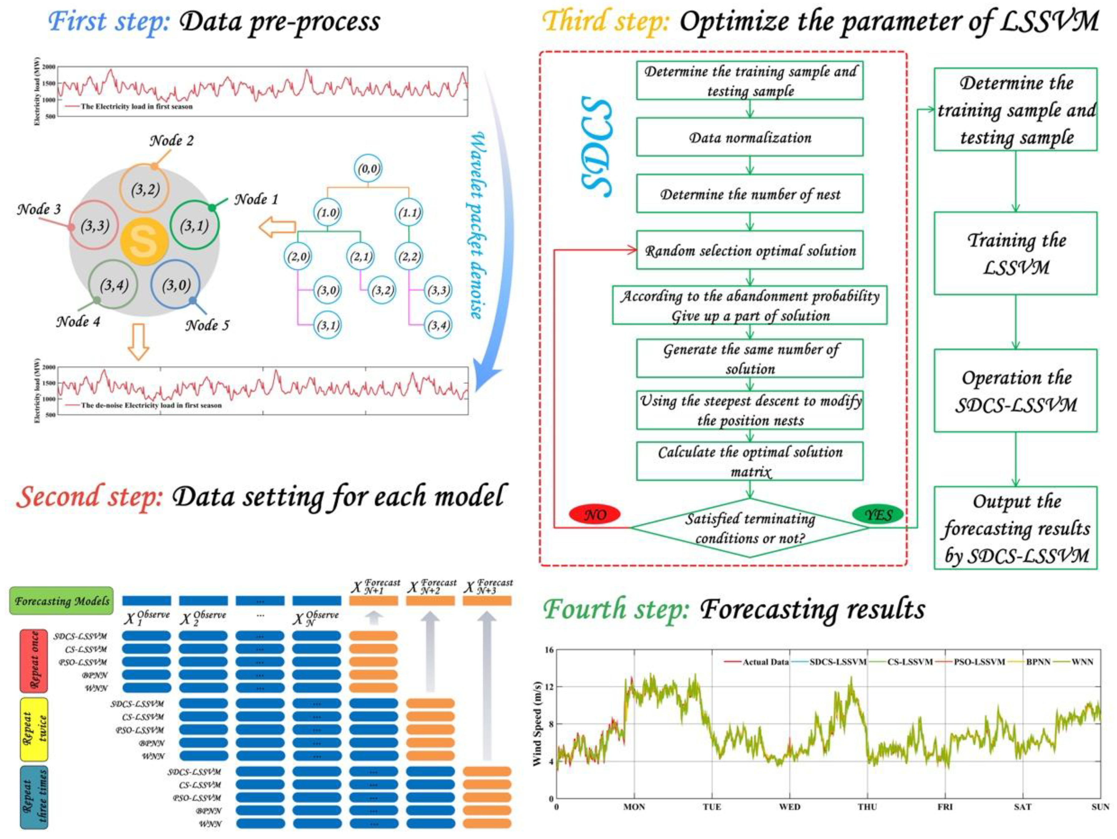
The wavelet packet transform extracts the multiscale spatial energy feature of the original wind speed. It is noteworthy that the applications of the wavelet packet transform need to select two hyperparameters: wavelet function and decomposition level. At present, no study discusses how to select the value of these two hyperparameters; their values can depend on the type of original wind speed time series to be analyzed. The procedure of the wavelet packet transform is displayed in Figure 1 (first step).

From Figure 1 (second step), the data setting for each model with length N (the number of the training sample) is fixed according to the original time series. For example, suppose the last 144 points of the wind speed time series with length of 1152 (N = 1008) will be forecasted, and the data structure is shown in Figure 1 (second step).

It must be noted that there is one step ahead of forecasting h = 1 of different wind farm sites in this paper.

After the wavelet packet transform, the filtered wind speed time series is input to the optimized least squares support vector machine. The overall flowchart of the proposed hybrid forecasting model is shown in Figure 1 (third step).

It is remarkable that the original wind speed time series divides into a training sample and a testing sample. Moreover, in the process of training the least squares support vector machine, the input data is filtered time series and the output data is original wind speed time series of the training sample, and in the testing process, the input data is also filtered time series and the output is test sample.

3. Numerical Experimentation

The wind farm is located between 120°43′6″ and 120°47′17″ north latitude and between 37°32′50″ and 37°37′6″ west longitude; the ground elevation is 140–420 m; and the annual average wind speed is higher than the surrounding region but also reserves the larger number of wind energy resources. In this region, the installed wind power capacity is approximately 67 million KW. The data collected in this paper are from 1 January 2015 to 31 March 2017. The data collected from 1 January 2015 to 31 March 2017 are used to analyzed wind energy resource and 1–12 March 2017 are used for wind speed forecasting. NRG # 40 and NRG # 200P wind speed sensors are installed at 70 m heights in the wind tower of the four different sites.

3.1. Analysis of Wind Speed

The probability distribution of wind speed can be used to measure the distribution of wind energy resources in a place. The common probability distributions are normal, Reyleigh, gamma, and Weibull, which use the distribution function to fit the probability distribution of wind speed. In this paper, four kinds of probability distribution are used to assess wind speed density. Figure 2 and the Appendix A (

Table A1. The assessment result by each hybrid Weibull distribution

Site 1					Site 2
Index	DE-Weibul	PSO-Weibul	CS-Weibul	GA-Weibul	DE-Weibul	PSO-Weibul	CS-Weibul	GA-Weibul
c	7.24378	7.26016	7.13038	7.13488	6.19191	6.26273	6.23039	6.09700
k	2.02080	1.98773	2.06653	2.07307	2.18602	2.14876	2.14211	2.20157
SSE	0.01632	0.01626	0.01506	0.01536	0.05491	0.05252	0.05284	0.05723
RMSE	0.01354	0.01352	0.01301	0.01314	0.02392	0.02339	0.02346	0.02442
R-square	0.97738	0.98256	0.98266	0.98005	0.95280	0.95711	0.96391	0.95490
Index	DE-Gamma	PSO-Gamma	CS-Gamma	GA-Gamma	DE-Gamma	PSO-Gamma	CS-Gamma	GA-Gamma
a	3.56657	3.57455	3.60064	3.60301	3.77476	3.79123	3.79374	3.77880
b	1.87786	1.87901	1.84529	1.84399	1.54797	1.54352	1.54849	1.53806
SSE	0.01532	0.01531	0.01572	0.01574	0.04669	0.04672	0.04641	0.04725
RMSE	0.01312	0.01311	0.01329	0.01330	0.02205	0.02206	0.02199	0.02219
R-square	0.91282	0.91261	0.91225	0.91221	0.92084	0.92384	0.94539	0.92447
Index	DE-Rayleigh	PSO-Rayleigh	CS-Rayleigh	GA-Rayleigh	DE-Rayleigh	PSO-Rayleigh	CS-Rayleigh	GA-Rayleigh
c	5.12560	5.12564	5.12573	5.12512	4.56307	4.56658	4.56838	4.57726
k	2	2	2	2	2.00000	2.00000	2.00000	2.00000
SSE	0.01518	0.01518	0.01518	0.01518	0.04597	0.04590	0.04586	0.04569
RMSE	0.01306	0.01306	0.01306	0.01306	0.02188	0.02187	0.02186	0.02182
R-square	0.92958	0.93269	0.94991	0.92141	0.91272	0.88876	0.90813	0.90626
Index	DE-Normal	PSO-Normal	CS-Normal	GA-Normal	DE-Normal	PSO-Normal	CS-Normal	GA-Normal
Sigma	6.60682	6.65526	6.59154	6.65188	5.79198	5.79547	5.79547	5.79826
mu	6.56244	6.53053	6.54393	6.56223	5.98361	5.99629	5.95254	5.96912
SSE	0.01334	0.01331	0.01335	0.01331	0.01958	0.01955	0.01955	0.01953
RMSE	0.01224	0.01223	0.01225	0.01223	0.01428	0.01427	0.01427	0.01426
R-square	0.74592	0.74801	0.77220	0.76017	0.76980	0.77130	0.76817	0.77435
Site 3					Site 4
Index	DE-Weibul	PSO-Weibul	CS-Weibul	GA-Weibul	DE-Weibul	PSO-Weibul	CS-Weibul	GA-Weibul
c	6.37829	6.33251	6.27264	6.33395	6.46472	6.49129	6.39166	6.42345
k	2.22638	2.15944	2.20120	2.15483	2.17758	2.14127	2.22021	2.14161
SSE	0.06692	0.06403	0.06584	0.06421	0.05832	0.05668	0.06110	0.05785
RMSE	0.02525	0.02469	0.02504	0.02473	0.02346	0.02312	0.02401	0.02336
R-square	0.97257	0.93699	0.94528	0.94239	0.94954	0.93142	0.92395	0.91892
Index	DE-Gamma	PSO-Gamma	CS-Gamma	GA-Gamma	DE-Gamma	PSO-Gamma	CS-Gamma	GA-Gamma
a	3.80404	3.79334	3.81104	3.82185	3.73173	3.72363	3.75314	3.73567
b	1.58183	1.58095	1.57419	1.57621	1.63625	1.63778	1.62564	1.63107
SSE	0.05680	0.05705	0.05720	0.05688	0.04873	0.04877	0.04900	0.04896
RMSE	0.02326	0.02331	0.02334	0.02327	0.02144	0.02145	0.02150	0.02149
R-square	0.84404	0.85837	0.87237	0.84624	0.86150	0.88755	0.88417	0.86390
Index	DE-Rayleigh	PSO-Rayleigh	CS-Rayleigh	GA-Rayleigh	DE-Rayleigh	PSO-Rayleigh	CS-Rayleigh	GA-Rayleigh
c	4.65629	4.65657	4.65687	4.65498	4.79502	4.80241	4.80554	4.81040
k	2	2	2	2	2.00000	2.00000	2.00000	2.00000
SSE	0.05539	0.05538	0.05538	0.05542	0.04887	0.04874	0.04869	0.04860
RMSE	0.02297	0.02297	0.02297	0.02297	0.02147	0.02144	0.02143	0.02141
R-square	0.86660	0.87685	0.90521	0.89792	0.84262	0.86562	0.84090	0.83779
Index	DE-Normal	PSO-Normal	CS-Normal	GA-Normal	DE-Normal	PSO-Normal	CS-Normal	GA-Normal
Sigma	5.88713	5.90077	5.90206	5.90469	6.06350	6.08123	6.08189	6.08744
mu	6.09282	6.09702	6.07053	6.08674	6.15987	6.15519	6.14823	6.13623
SSE	0.02427	0.02415	0.02414	0.02412	0.02199	0.02185	0.02185	0.02181
RMSE	0.01520	0.01517	0.01516	0.01516	0.01440	0.01436	0.01436	0.01434
R-square	0.75443	0.71644	0.73388	0.73280	0.69514	0.70012	0.70575	0.69116

) show that the Weibull distribution well fits the distribution of wind speed. For example, the R-square of four probability distributions at Site 1 are 0.918, 0.768, 0.831, and 0.765. In the assessment of Site 2 processing, the Weibull distribution also well fits the wind speed distribution, which the sum square error (SSE) of Weibull distribution is 0.876 lower than the other distributions. The doughnut in Figure 2 shows the capacity factor of each site, with values of 35.860%, 27.456%, 26.825%, and 28.738%. In order to accurately assess wind speed, four different optimization algorithms are used to optimize the parameters of the Weibull distribution. From Appendix A (Table A1) we can clearly see that the optimal Weibull distributions are obtained by different optimizations; the optimal Weibull distribution for Site 1 is CS-Weibull and the other optimal Weibull distributions are shown in the Appendix A (Table A1), marked in bold.

In this paper, four data sites have been selected as our case studies. The sites’ wind characteristics and Weibull parameters are estimated using the above expressions for all locations considered in the present study and are presented in

Table 2. The different sites wind speed characteristics and Weibull parameters.

Index	CS-Weibull	CS-Weibull	DE-Weibull	DE-Weibull
vm (m/s)	6.5214	5.8752	5.9730	6.1713
c	7.13038	6.23039	6.37829	6.46472
k	2.06653	2.14211	2.22638	2.17758
SSE	0.01506	0.05284	0.06692	0.05832
RMSE	0.01301	0.02346	0.02525	0.02346
R-square	0.98266	0.96391	0.97257	0.94954
vf(m/s)	5.17729	4.64524	4.87960	4.87466
ve(m/s)	9.89400	8.47629	8.50622	8.71942
Capacity factor	35.860%	26.825%	27.456%	28.738%
p(v)(KW/m2)	904.4035	661.3063	694.8981	766.4413

. The table shows that the annual mean wind speeds are 6.5214 m/s, 5.8752 m/s, 5.9730 m/s, and 6.1713 m/s for the four sites. Also displayed in Table 2 is the shape parameter of Weibull for the four sites. It can be seen that the shape parameter varies between 2.07 and 2.23 for these sites. It can further be noted that the annual wind speed carrying maximum energy speeds are 9.89400 m/s, 8.47629 m/s, 8.50622 m/s, and 8.71942 m/s. Furthermore, the annual mean power densities are 904.4035 KW/m², 661.3063 KW/m², 694.8981 KW/m², and 766.4413 KW/m² for the four sites.

The analysis of the wind energy resources and power generation of a wind turbine at four wind-speed sites shows that the capacity factor of wind turbine generation is 35.860%, 26.825%, 27.456%, and 28.738%. To reduce the operational cost of a wind farm, it is very important to improve the short-term wind speed forecasting accuracy. This section focuses on establishing the accuracy of the short-term wind-speed forecasting model and analyzing the forecasting results.

3.2. Definition of the Performance Metrics

To demonstrate the validity of the proposed hybrid model, three error measurements [27], mean absolute percentage error (MAPE), mean relative error (MRE), mean absolute error (MAE), and root mean squared error (RMSE), are used to evaluate the accuracy and stability of forecasting results. MAPE, MRE, and MAE are used to evaluate accuracy. RMSE is used to measure the stability of the model, and a positive value of P_bias [28] denotes underestimation of bias, while a negative value denotes overestimation of bias. P_bias = 0 indicates no bias. They are calculated in

Table 3. The model evaluation metric.

Metric	Description	Equation
MAE	Mean Absolute Error	MAE =$\frac{1}{N}{{\displaystyle \sum }}_{i=1}^n|y_i-{\widehat{y}}_i|$
MRE	Mean Relative Error	MRE =$\frac{NMAE}{{{\displaystyle \sum }}_{i=1}^N\left|y_i\right|}\times 100\%$
RMSE	Root Mean Squared Error	RMSE =$\sqrt{\frac{1}{N}{{\displaystyle \sum }}_{i=1}^n{\left|y_i-{\widehat{y}}_i\right|}^2}$
MAPE	Mean Absolute Percentage Error	MAPE =$\frac{1}{N}{{\displaystyle \sum }}_{i=1}^n\left|\frac{y_i-{\widehat{y}}_i}{y_i}\right|\times 100\%$
IA	Index Agreement [29]	IA =$1-\frac{{{\displaystyle \sum }}_{i=1}^N(y_i-{\widehat{y}}_i{)}^2}{{{\displaystyle \sum }}_{i=1}^N\left(\right|y_i-{\widehat{y}}_i|+|y_i-\stackrel{-}{y}|{)}^2}$
Pbias	Percent bias	Pbias=$\frac{{{\displaystyle \sum }}_{i=1}^N(y_i-{\widehat{y}}_i)}{{{\displaystyle \sum }}_{i=1}^N-{\widehat{y}}_i}$

as follows.

3.3. Data Setting for Each Model

The actual wind speed series from the four observation stations and their assessment results are shown in Figure 2. According to the above analysis, the capacity factor is about 35.860%, 26.825%, 27.456%, and 28.738% for each site. In order to improve the utilization of wind energy, it is necessary to accurately forecast wind speed.

In this paper, all of the wind speed data in the sampling period is taken over 8 days, including 1152 data points in two parts, training sample and testing sample. In order to ensure that the training set gets more information between the input variables and the output variables, the first 1008 wind speed data points serve as the training set, and last 144 data points serve as the testing sample. The training sample is processed by wavelet packet transform (WPT) and the testing sample is actual wind speed time series, and they are shown in

Table 4. The best parameter of LSSVM for different Sites.

Site	Site 1	Site 2	Site 3	Site 4
Kernel function	RBF_kernel	RBF_kernel	RBF_kernel	RBF_kernel
Input Data Type	De-noise	De-noise	De-noise	De-noise
No. Input	4	8	7	4
Output Data Type	Actual	Actual	Actual	Actual
No. Output	1	1	1	1
Gam	11.368	7.063	13.415	15.133
Sig2	0.1	0.1	0.1	0.1

. In order to ensure the best proportion between the training and testing samples, the enumeration method based on numerical simulation is used (the results are shown in Figure 3). The LSSVM parameters of the hybrid model are shown in Table 4.

To determine the relationship between the number of input and training samples, many experiments were established. In these experiments, we used the listing technique to determine the number of input and training samples for the different forecasting models. From Figure 3, the following conclusions were obtained:

(1)

Figure 3A and

Table 5. Forecasting results in Site 1 for a week.

Week	Model	MAE	MRE	RMSE	MAPE	IA	Pbias
Mon	SDCS-LSSVM	0.1991	3.10%	0.2656	3.11%	0.9986	0.91%
	CS-LSSVM	0.3425	5.34%	0.4399	5.85%	0.9905	0.97%
	PSO-LSSVM	0.3699	5.77%	0.4707	6.20%	0.9891	1.05%
	SDCS-BPNN	0.3656	5.70%	0.5166	5.98%	0.9899	1.17%
	SDCS-WNN	0.5285	8.24%	0.7100	8.90%	0.9762	1.48%
Tue	SDCS-LSSVM	0.1017	0.94%	0.1324	1.01%	0.9995	0.05%
	CS-LSSVM	0.3832	3.54%	0.5023	3.58%	0.9918	−0.23%
	PSO-LSSVM	0.3993	3.69%	0.5272	3.71%	0.9908	0.26%
	SDCS-BPNN	0.3852	3.56%	0.5087	3.57%	0.9954	−0.29%
	SDCS-WNN	0.5390	4.98%	0.6782	5.04%	0.9880	−0.61%
Wed	SDCS-LSSVM	0.0978	1.77%	0.1168	1.79%	0.9977	−0.18%
	CS-LSSVM	0.2538	4.60%	0.3143	4.65%	0.9817	−0.21%
	PSO-LSSVM	0.2589	4.69%	0.3510	4.74%	0.9774	0.33%
	SDCS-BPNN	0.2505	4.54%	0.3101	4.62%	0.9851	−0.80%
	SDCS-WNN	0.3531	6.40%	0.4598	6.36%	0.9617	−0.90%
Thu	SDCS-LSSVM	0.1329	1.76%	0.1750	1.76%	0.9986	−0.21%
	CS-LSSVM	0.3782	5.01%	0.4844	5.14%	0.9889	0.23%
	PSO-LSSVM	0.3734	4.95%	0.4784	5.14%	0.9892	−0.33%
	SDCS-BPNN	0.3607	4.78%	0.4624	4.89%	0.9938	−0.32%
	SDCS-WNN	0.5062	6.71%	0.6813	6.71%	0.9796	0.41%
Fri	SDCS-LSSVM	0.1098	2.10%	0.1446	2.15%	0.9964	−0.09%
	CS-LSSVM	0.2995	5.74%	0.3795	5.73%	0.9721	0.18%
	PSO-LSSVM	0.3020	5.79%	0.3797	5.77%	0.9715	0.33%
	SDCS-BPNN	0.2928	5.62%	0.3621	5.71%	0.9747	0.35%
	SDCS-WNN	0.4307	8.26%	0.5484	8.24%	0.9374	−0.48%
Sat	SDCS-LSSVM	0.1055	1.62%	0.1385	1.67%	0.9960	−0.08%
	CS-LSSVM	0.2472	3.80%	0.3173	4.05%	0.9758	−0.10%
	PSO-LSSVM	0.2521	3.88%	0.3196	4.11%	0.9747	−0.27%
	SDCS-BPNN	0.2470	3.80%	0.3150	4.04%	0.9779	−0.56%
	SDCS-WNN	0.3630	5.58%	0.4735	5.80%	0.9455	0.57%
Sun	SDCS-LSSVM	0.0729	0.95%	0.0995	0.96%	0.9991	−0.34%
	CS-LSSVM	0.2339	3.04%	0.2995	3.12%	0.9916	0.35%
	PSO-LSSVM	0.2433	3.16%	0.3062	3.21%	0.9911	0.45%
	SDCS-BPNN	0.2335	3.04%	0.2912	3.10%	0.9960	0.61%
	SDCS-WNN	0.3142	4.08%	0.4039	4.17%	0.9878	0.74%

show that the forecasting performance of WPT-SDCS-LSSVM is better than the other four models, in which the value of MAPE of 3.45% is lower than the other hybrid model. Figure 3B shows that the forecasting curve obtained by WPT-SDCS-LSSVM is very close to the original wind speed time series.

(2)

Figure 3C shows that the range of input for each forecasting model is 1–30, in which the MAPE range of WPT-SDCS-LSSVM is 3.45–7.5%. When the number of inputs increases, the test error gradually decreases. If the number of inputs reaches a certain maximum, the test error will increase. Table 4 shows the best input for LSSVM, and Figure 3C shows that the change of training sample size corresponds to the change of test accuracy, and it can be clearly seen that with the increase of training samples, the accuracy of the WPT-SDCS-LSSVM is improved and the fluctuation range of accuracy is between 5.5% and 7.5%.

Remark 1.

According to the above analysis, it is discovered that it is hard to find the general relationship between the number of the input layer and the training sample. Wind speed time series at different sites have different forecasting structures, which suggests that different time series corresponding to the parameters of the model are also different.

3.4. Numerical Simulation for Four Different Sites

In this section, to illustrate the effectiveness of the hybrid model, we will compare three models: back propagation neural network (BPNN), wavelet neural network (WNN), CS-LSVM, and PSO-LSSVM. Table 5,

Table 6. The forecasting result in Site 2 for a week.

Week	Model	MAE	MRE	RMSE	MAPE	IA	Pbias
Mon	SDCS-LSSVM	0.3434	4.66%	0.4343	5.00%	0.9909	0.489%
	CS-LSSVM	0.3599	4.89%	0.4519	5.16%	0.9901	0.643%
	PSO-LSSVM	0.3587	4.87%	0.4540	5.18%	0.9901	0.694%
	SDCS-BPNN	0.4874	6.62%	0.6040	7.06%	0.9789	1.168%
	SDCS-WNN	0.5218	7.09%	0.6865	7.42%	0.9784	1.277%
Tue	SDCS-LSSVM	0.4116	3.52%	0.5161	3.57%	0.9907	−0.133%
	CS-LSSVM	0.4307	3.69%	0.5359	3.74%	0.9898	−0.221%
	PSO-LSSVM	0.4311	3.69%	0.5427	3.74%	0.9896	−0.243%
	SDCS-BPNN	0.5423	4.64%	0.6853	4.69%	0.9860	−0.289%
	SDCS-WNN	0.5573	4.77%	0.7015	4.86%	0.9854	−0.343%
Wed	SDCS-LSSVM	0.2570	3.90%	0.3198	3.99%	0.9759	0.108%
	CS-LSSVM	0.2621	3.98%	0.3215	4.05%	0.9759	−0.299%
	PSO-LSSVM	0.2616	3.97%	0.3262	4.07%	0.9748	−0.403%
	SDCS-BPNN	0.3500	5.32%	0.4241	5.54%	0.9545	−0.410%
	SDCS-WNN	0.3657	5.55%	0.4620	5.67%	0.9479	−1.016%
Thu	SDCS-LSSVM	0.3743	3.99%	0.4815	3.95%	0.9903	0.012%
	CS-LSSVM	0.3737	3.99%	0.4660	3.98%	0.9883	0.127%
	PSO-LSSVM	0.3770	4.02%	0.4836	3.99%	0.9873	0.264%
	SDCS-BPNN	0.5193	5.54%	0.6662	5.49%	0.9766	0.281%
	SDCS-WNN	0.5312	5.67%	0.6940	5.74%	0.9755	0.486%
Fri	SDCS-LSSVM	0.2721	4.72%	0.3453	4.79%	0.9810	0.036%
	CS-LSSVM	0.2792	4.84%	0.3520	4.92%	0.9802	0.163%
	PSO-LSSVM	0.2860	4.96%	0.3591	4.99%	0.9793	0.280%
	SDCS-BPNN	0.3867	6.71%	0.4819	6.87%	0.9583	−0.323%
	SDCS-WNN	0.3985	6.91%	0.5253	6.94%	0.9566	−0.618%
Sat	SDCS-LSSVM	0.2774	3.54%	0.3481	3.65%	0.9802	0.047%
	CS-LSSVM	0.2786	3.55%	0.3541	3.66%	0.9796	−0.098%
	PSO-LSSVM	0.2854	3.64%	0.3700	3.72%	0.9779	0.162%
	SDCS-BPNN	0.3773	4.81%	0.4770	4.96%	0.9577	−0.308%
	SDCS-WNN	0.3967	5.06%	0.5197	5.24%	0.9551	0.395%
Sun	SDCS-LSSVM	0.2357	2.78%	0.3085	2.75%	0.9914	0.314%
	CS-LSSVM	0.2535	2.99%	0.3462	2.97%	0.9890	0.520%
	PSO-LSSVM	0.2676	3.16%	0.3713	3.11%	0.9871	0.669%
	SDCS-BPNN	0.3015	3.56%	0.4212	3.50%	0.9891	0.898%
	SDCS-WNN	0.3164	3.74%	0.4226	3.64%	0.9869	1.103%

,

Table 7. The forecasting result in Site 3 for a week.

Week	Model	MAE	MRE	RMSE	MAPE	IA	Pbias
Mon	SDCS-LSSVM	0.3055	4.332%	0.4154	4.478%	0.9980	0.302%
	CS-LSSVM	0.3595	4.964%	0.5267	5.768%	0.9848	1.028%
	PSO-LSSVM	0.3574	5.615%	0.5406	5.362%	0.9724	0.945%
	SDCS-BPNN	0.4663	6.671%	0.6516	6.691%	0.9452	3.124%
	SDCS-WNN	0.5047	7.157%	0.6764	7.565%	0.9453	2.657%
Tue	SDCS-LSSVM	0.5092	4.364%	0.6223	4.413%	0.9976	0.105%
	CS-LSSVM	0.5696	4.810%	0.6688	4.854%	0.9892	−0.167%
	PSO-LSSVM	0.5582	4.676%	0.7996	4.986%	0.9736	−0.281%
	SDCS-BPNN	0.6340	5.433%	0.7736	5.555%	0.9673	−0.478%
	SDCS-WNN	0.6891	6.007%	0.8298	6.003%	0.9633	−0.401%
Wed	SDCS-LSSVM	0.2513	3.772%	0.3071	3.919%	0.9983	0.015%
	CS-LSSVM	0.2656	4.782%	0.3530	4.143%	0.9824	0.082%
	PSO-LSSVM	0.2925	4.474%	0.3563	4.705%	0.9837	0.025%
	SDCS-BPNN	0.3359	4.939%	0.4049	5.176%	0.9782	−0.279%
	SDCS-WNN	0.3535	5.307%	0.4539	5.470%	0.9775	−0.269%
Thu	SDCS-LSSVM	0.3839	4.136%	0.5131	4.070%	0.9978	−0.063%
	CS-LSSVM	0.4463	4.632%	0.6101	4.799%	0.9872	−0.202%
	PSO-LSSVM	0.4713	4.759%	0.6073	4.711%	0.9702	0.238%
	SDCS-BPNN	0.5503	5.928%	0.7567	5.673%	0.9668	0.543%
	SDCS-WNN	0.6602	6.687%	0.9184	6.658%	0.9643	0.729%
Fri	SDCS-LSSVM	0.2989	5.122%	0.3940	5.121%	0.9965	−0.050%
	CS-LSSVM	0.3230	6.178%	0.4308	5.912%	0.9866	−0.223%
	PSO-LSSVM	0.3277	6.223%	0.4369	6.433%	0.9808	−0.357%
	SDCS-BPNN	0.4085	6.856%	0.5236	6.886%	0.9778	0.412%
	SDCS-WNN	0.4347	7.449%	0.5948	7.455%	0.9759	0.324%
Sat	SDCS-LSSVM	0.3016	4.128%	0.4007	4.261%	0.9977	−0.063%
	CS-LSSVM	0.3164	4.965%	0.5029	4.921%	0.9881	−0.123%
	PSO-LSSVM	0.3689	4.976%	0.4567	5.092%	0.9859	0.301%
	SDCS-BPNN	0.3992	5.558%	0.5602	5.707%	0.9782	0.470%
	SDCS-WNN	0.4061	5.658%	0.5581	5.839%	0.9700	−0.999%
Sun	SDCS-LSSVM	0.2683	3.164%	0.3469	3.159%	0.9988	0.122%
	CS-LSSVM	0.3026	3.791%	0.3551	3.765%	0.9858	0.202%
	PSO-LSSVM	0.3417	3.938%	0.3580	3.754%	0.9841	0.225%
	SDCS-BPNN	0.3548	4.151%	0.4551	4.287%	0.9776	0.260%
	SDCS-WNN	0.3907	4.607%	0.4953	4.549%	0.9752	0.592%

and

Table 8. The probability of forecasting error in different intervals.

Interval	[−4, −3.2)	[−3.2, −2.4)	[−2.4, −1.6]	[−1.6, −0.8)	[−0.8, 0)	[0, 0.8)	[0.8, 1.6)	[1.6, 2.4)	[2.4, 3.2)
SDCS-LSSVM	0	0	0.00496	0.041667	0.46627	0.450397	0.036706	0	0
CS-LSSVM	0	0.000992	0.007937	0.077381	0.429563	0.424603	0.054563	0.00496	0
PSO-LSSVM	0.000992	0.001984	0.011905	0.083333	0.39881	0.406746	0.085317	0.010913	0
BPNN	0	0	0.01291	0.073486	0.385303	0.446872	0.070506	0.008937	0.001986
WNN	0	0.000992	0.00496	0.065476	0.415675	0.44246	0.065476	0.003968	0.000992

and Figure 4, Figure 5, Figure 6 and Figure 7 show the forecasting results of the hybrid model at four sites.

3.4.1. The Forecasting Result in Site 1

From Table 5, it is clear that the WPT-CS-LSSVM model performs much better than the other three models. To explain the results of the proposed method, we utilize the first site as an example. First, the hybrid LSSVM model has the smallest statistical error of MAPE, RMSE, MAE, and MRE when compared with the other three models. For example, in

Table 9. The forecasting result in Site 4 for a week.

Week	Model	MAE	MRE	RMSE	MAPE	IA	Pbias
Mon	SDCS-LSSVM	0.2958	4.55%	0.3721	5.01%	0.9917	−0.18%
	CS-LSSVM	0.3679	5.66%	0.4769	6.03%	0.9824	−0.38%
	PSO-LSSVM	0.3851	5.93%	0.4992	6.31%	0.9806	0.39%
	SDCS-BPNN	0.4330	6.67%	0.5614	7.10%	0.9746	−0.41%
	SDCS-WNN	0.4940	7.60%	0.6405	8.10%	0.9665	−0.55%
Tue	SDCS-LSSVM	0.5658	5.48%	0.7356	5.62%	0.9813	−0.08%
	CS-LSSVM	0.5811	5.63%	0.7819	6.51%	0.9869	0.21%
	PSO-LSSVM	0.5860	5.68%	0.7778	6.87%	0.9832	−0.42%
	SDCS-BPNN	0.5717	5.54%	0.7386	7.33%	0.9810	−0.78%
	SDCS-WNN	0.7190	6.96%	0.9211	7.12%	0.9714	−1.25%
Wed	SDCS-LSSVM	0.2585	4.15%	0.3548	4.26%	0.9821	0.24%
	CS-LSSVM	0.2582	4.15%	0.3516	5.30%	0.9785	0.27%
	PSO-LSSVM	0.2614	4.20%	0.3604	5.65%	0.9741	0.41%
	SDCS-BPNN	0.2726	4.38%	0.3680	6.37%	0.9688	0.58%
	SDCS-WNN	0.4184	6.72%	0.5587	6.94%	0.9247	0.78%
Thu	SDCS-LSSVM	0.4236	5.19%	0.5695	5.26%	0.9806	0.02%
	CS-LSSVM	0.4540	5.56%	0.6242	6.89%	0.9788	−0.09%
	PSO-LSSVM	0.4586	5.62%	0.6360	7.12%	0.9769	0.20%
	SDCS-BPNN	0.2590	4.16%	0.3496	6.05%	0.9736	0.55%
	SDCS-WNN	0.3975	6.39%	0.5308	6.59%	0.9294	0.74%
Fri	SDCS-LSSVM	0.2926	5.24%	0.4029	5.45%	0.9606	0.06%
	CS-LSSVM	0.2987	5.35%	0.4141	6.47%	0.9591	−0.28%
	PSO-LSSVM	0.3047	5.46%	0.4180	6.76%	0.9573	−0.30%
	SDCS-BPNN	0.2970	5.32%	0.4050	7.80%	0.9615	0.59%
	SDCS-WNN	0.4427	7.93%	0.6038	8.34%	0.9589	0.74%
Sat	SDCS-LSSVM	0.2613	3.52%	0.3250	3.62%	0.9868	0.17%
	CS-LSSVM	0.2665	3.59%	0.3359	4.78%	0.9759	0.23%
	PSO-LSSVM	0.2694	3.63%	0.3334	4.55%	0.9781	0.38%
	SDCS-BPNN	0.2610	3.51%	0.3254	5.34%	0.9706	0.52%
	SDCS-WNN	0.4130	5.56%	0.5145	5.66%	0.9675	0.88%
Sun	SDCS-LSSVM	0.3019	3.97%	0.3956	3.93%	0.9855	0.55%
	CS-LSSVM	0.3120	4.11%	0.4033	5.27%	0.9762	0.17%
	PSO-LSSVM	0.3213	4.23%	0.4131	5.33%	0.9536	0.23%
	SDCS-BPNN	0.3219	4.24%	0.4100	5.58%	0.9534	0.36%
	SDCS-WNN	0.4435	5.84%	0.5864	5.72%	0.9505	0.88%

, the MAPE of our hybrid method is 4.50% while the single BPNN is calculated to be 5.65%; thus, the precision is improved by 1.16%. In the remaining models, the precision is improved by 4.91% and 2.56%. This result combines the advantages of each single model. Second, the various indicators of the hybrid LSSVM model are better than PSO-LSSVM. The major cause for this, among others, is that the hybrid model consists of WPT and CS. This illustrates that WPT and SDCS are more effective than PSO. Not only that, the run time of SDCS is much shorter than PSO at the Site 1, as shown in Table 5. On the whole, the hybrid LSSVM model is quite simple and efficient.

As mentioned earlier, Figure 4A shows that the forecasting error of SDCS-LSSVM is approximately 0. Table 5 and Figure 4B show that the MAE, MRE, RMSE, and MAPE values of SDCS-LSSVM are 0.1991, 3.10%, 0.2656, and 3.11%, respectively, which are lower than the other model, and the Index Agreement of SDCS-LSSVM is 0.9986, closed to 1, which is higher than the other model. Figure 4C shows the 95% confidence intervals (CIs) obtained by the proposed hybrid model (SDCS-LSSVM), which indicate that both the upper and lower CI are close to the observed wind speed time series. Table 5 shows that single models cannot be applied to multiple forecasting problems, and model performance under specific conditions should be analyzed and understood and incremental improvements made based on knowledge gained [30,31,32,33,34]. In this paper, our hybrid LSSVM model based on WPT and SDCS performs much better than the single models in terms of its precision and stability, and is an excellent method for 10-min wind speed forecasting in Shandong Province compared with other traditional forecasting models.

3.4.2. The Forecasting Result in Site 2

The cuckoo search algorithm easily suffers from slow convergence, which will affect its parameter optimization capability. Therefore, the steepest descent algorithm is used to iterate and modify the location of the nest to obtain the optimal parameters. The SDCS algorithm combines the advantages of the steepest descent algorithm and the cuckoo search algorithm, which significantly improves the convergence speed of the cuckoo algorithm. The forecasting results can be seen in Figure 5A, and Table 6 shows that this proposed WPT-SDCS-LSSVM model outperforms the other four hybrid models comparing the MAE, MRE, RMSE, MAPE, IA, and P_bias from Monday to Sunday. For instance, the MAPE of the WPT-SDCS-LSSVM is 5.00%, 3.57%, 3.99%, 3.95%, 4.79%, 3.65%, and 2.75%, corresponding to P_bias of 0.489%, −0.133%, 0.108%, 0.012%, 0.036%, 0.047%, and 0.314% from Monday to Sunday, respectively. Figure 5A and Table 6 show that the IA values of 0.9909, 0.9907, 0.9759, 0.9903, 0.9810, 0.9802, and 0.9914 obtained by WPT-SDCS-LSSVM are bigger than the other models. Forecasting values of all models are shown in Figure 5A. It is demonstrated that this proposed hybrid model has high accuracy and low bias. However, the IA values are 0.9986, 0.9995, 0.9977, 0.9986, 0.9964, 0.996, and 0.9991 from Monday to Sunday. It is also shown that the WPT-SDCS-LSSVM can accurately forecast future changes in wind speed.

In order to analyze the forecasting results of the five models, we used the testing set from Monday to Sunday. Figure 5A clearly displays the forecasting values and actual values of 00:10 to 24:00, from Monday to Sunday, 6–12 March 2017, in which all models obtained the best forecasting accuracy in the forecasting of Sunday. Figure 5B.1 shows the values of the five forecasting models and the actual wind speed from 00:10 to 24:00, Sunday, 12 March 2017. Figure 5B.2 shows 95% confidence intervals (CIs) obtained by the WPT-SDCS-LSSVM. It can be clearly seen that both the upper and lower CIs are very close to the actual wind speed time series of Sunday. Figure 5B.3 is the plot of forecasting values from 00:10 to 24:00, Sunday, 12 March 2017, for these five forecasting models. It can be seen that the performance of the WPT-SDCS-LSSVM is better than two single models and two hybrid models. In addition, Table 6 clearly shows the metrics of the five forecasting models which find the three forecasting (LSSVM, BPNN, and WNN) models are optimized by the same optimization algorithm (SDCS), and the forecasting performance of SDCS-LSSVM is better than the other two hybrid forecasting models (SDCS-BPNN and SDCS-WNN). It is obvious that the forecasting values of the proposed WPT-SDCS-LSSVM hybrid model is approximate to the actual wind speed time series.

3.4.3. The Forecasting Result in Site 3

For the Site 3 forecasting process, Figure 6A clearly shows the forecasting metric values of MAE, MRE, RMSE, and MAPE, in which the proposed hybrid obtains the minimum values of 0.3055, 4.332%, 0.4154, and 4.478%, respectively, on Monday. At the same time, the proposed model obtains a maximum IA (0.9980) and minimum P_bias (0.302%), which indicates that WPT-SDCS-LSSVM can provide a more accurate and stable forecasting value. Figure 6B shows the performance of each hybrid model and plots the forecasting performance, forecasting value, and forecasting error for the five hybrid models at Site 3. Figure 6B shows that the forecasting value of WPT-SDCS-LSSVM falls within the 95% confidence interval of the original wind speed. Figure 6B clearly shows the actual wind speed compared with the forecasting values (with 95% confidence intervals) for Site 3. It shows that the 95% confidence interval obtained by the proposed hybrid model (WPT-SDCS-LSSVM) is narrower than those of the other hybrid models. It is shown for a week of forecasting values. From Figure 6B, it can be seen that the distribution forecasting error of WPT-SDCS-LSSVM is lower than that of the other hybrid model.

In Figure 6B, the probability distribution of forecasting error shows the distribution of forecasting error (FE) for SDCS-LSSVM, CS-LSSVM, PSO-LSSVM, BPNN, and WNN at Site 3, where FE is defined as FE = $x_i^{actual}{-x}_i^{forecast}$, $x_i^{ctual}$, and $x_i^{forecast}$ representing the actual wind speed time series and forecasting wind speed time series. Figure 6B show the probability of forecasting error in different intervals and the distribution forecasting error produced by each forecasting model, which indicates that the probability interval of each model is mainly between −0.8 and 0.8, and the probabilities (between [−0.8, 0.8]) of SDCS-LSSVM, CS-LSSVM, PSO-LSSVM, BPNN, and WNN are 0.916667, 0.854166, 0.805556, 0.832175, and 0.858135, respectively.

Through the above forecasting error analysis, and combined with the forecasting metric in Table 7, we find that the proposed WPT-SDCS-LSSVM integrated model is better than the other model. In a nutshell, it can be explained that this proposed integrated algorithm has better capacity of location and global search to find optimizing regularization (Gam) and tuning parameter (Sig2) for nonlinear least squares support vector machine and wavelet packet transform as a preprocessing technique, which can extract tendency and volatility features in the original wind speed time series, improving forecasting accuracy. In addition, the nonlinear least squares support vector machine can effectively reduce forecasting error because the dataset structures are optimized by the longitudinal dataset selection approach.

Remark 2.

By comparing the hybrid model proposed in this paper with four other models (two hybrid models and two single models), we can conclude that the proposed hybrid model provides more accurate forecasting results. A comparison between WPT-SDCS-LSSVM, WPT-CS-LSSVM, and WPT-PSO-LSSVM suggests that the optimization ability of SDCS is stronger than the single cuckoo search algorithm and particle swarm optimization algorithm, while the forecasting performance of single forecasting model is worse than hybrid models.

3.4.4. The Forecasting Result in Site 4

(1)

Table 9 shows the forecasting performance of hybrid models for Site 4 by CS-LSSVM, PSO-LSSVM, BPNN, WNN, and SSDCS-LSSVM in one-step-ahead forecasting in terms of six criteria: MAE, MRE, RMSE, MAPE, IA, and P_bias. For one-step-ahead forecasting, the proposed hybrid model outperforms all of the other models based on the evaluation criteria. For example, from the forecasting results of Monday, we can see that the hybrid model has higher forecasting accuracy, with MAE, MRE, RMSE, and MAPE values of 0.2958, 4.554%, 0.3721, and 5.011%, respectively. IA and P_bias achieved by the proposed hybrid model are 0.9917 and –0.132%, respectively. The WPT-CS-LSSVM model is second in accuracy next to the proposed hybrid model, but WPT-WNN shows the worst forecasting performance among these models.

(2)

Figure 7A shows the forecasting values and actual values for Site 4 in a week. Figure 7A shows the MAE and RMSE of each model, which are clearly significant improvements for hybrid model forecasting compared with the results of other forecasting models in weekly forecasting at Site 4. For example, for the forecasting results on Monday, the MAE value of each model is 0.2958, 0.3679, 0.3851, 0.4558, and 0.5200, which the hybrid model WPT-SDCS-LSSVM leads to 24.37%, 30.19%, 54.09%, and 75.79% reductions in MAE, and the RMSE value of each model is 0.3721, 0.4769, 0.4992, 0.5909, and 0.6742, which indicates that the hybrid WPT-SDCS-LSSVM model leads to 28.16%, 34.16%, 58.80%, and 81.19% reductions in RMSE. Figure 7A shows that the IA value of each model is 0.9917, 0.9824, 0.9806, 0.9698, and 0.9617, which indicates that the hybrid model WPT-SDCS-LSSVM leads to 0.94%, 1.12%, 2.21%, and 3.03% improvement in IA. Figure 7A shows the MAPE, MRE, and P_bias values of SDCS-LSSVM, which are 5.011%, 4.554%, and −0.132%, respectively, in comparison to SDCS-LSSVM, CS-LSSVM, PSO-LSSVM, BPNN, and WNN. For weekly forecasting, the maximum decreases of MAE, RMSE, and MAPE from the proposed hybrid model are 75.79%, 75.78%, and 70.13%, respectively. Figure 7B shows the performance of each model, in which the R-square is 0.9512, 0.9454, 0.9456, 0.9045, and 0.8894 for weekly forecasting at Site 4.

Remark 3.

The level of improvement by the combined forecasting model decreased as the number of forecasting steps increased. In spite of this, the forecasting performance of the combined model showed great improvement compared with the other models. The combined model proposed in this paper obtains satisfactory results in terms of wind speed forecasting.

4. Discussion the Forecasting Accuracy for Each Model

Finally, the above criteria are some of the most common standards; in fact, these criteria cannot appropriately judge the effectiveness of the forecasting method. The reason is that the different index series have different dimensions, so these criteria cannot be used directly. Even for similar sequences that have the same dimensions, the same period index values are different, so the above standard cannot show that the forecasting methods are equally effective. Therefore, this paper uses forecasting effectiveness (FE) to supplement the above criteria.

We presume that the observation sequence value is {x_t, t = 1, 2, ∙∙∙, N} and ${\overline{x}}_t$ is the estimated value. The following concepts can be obtained:

Definition 1.

Let

$$\{\begin{array}{cc}-1& if(x_t-{\overline{x}}_t)/x_t<-1\\ (x_t-{\overline{x}}_t)/x_t& if-1\le (x_t-{\overline{x}}_t)/x_t\le 1\\ 1& if(x_t-{\overline{x}}_t)/x_t>1\end{array}$$

(8)

In this formula, e_t is relative forecasting error at time t, t = 1, 2, ⋯, N. Obviously, 0 ≤ |e_t| ≤ 1.

Definition 2.

Let A_t = 1 − |e_t| be forecasting accuracy at time t, t = 1, 2, ⋯, N. Obviously, 0 ≤ A_t ≤ 1; if $(x_t-{\overline{x}}_t)/x_t$ > 1, A_t = 0, and this shows that the forecasting method is invalid at time t.

From Definition 2, e_t has randomness, so {A_t, t = 1, 2, ∙∙∙, N} is a random variable sequence.

Definition 3.

Let m^k = ${{\displaystyle \sum }}_{t=1}^N{Q}_t{A}_t^k$ be the forecasting effectiveness element, k is a positive integer, and {Q_t, t = 1, 2, ⋯, N} is the discrete probability distribution of the forecasting method at time t. ${{\displaystyle \sum }}_{t=1}^N{Q}_t=1$, Q_t > 0.

If the discrete probability distribution is not ascertained, we can set Q_t = 1/N, t = 1,2, ∙∙∙, N.

Definition 4.

Let H be a k-dimensional continuous function, then H(m¹, m², ⋯, m^k) is k-order forecast effectiveness.

Definition 5.

If H(x) = x is a one-dimensional continuous function, H(m¹) = m¹ is one-order forecast effectiveness; if H(x, y) = x(1 − $\sqrt{{y-x}^2}$) is a two-dimensional continuous function, H(m¹, m²) = x(1 − $\sqrt{m^2{-(m}^1{)}^2}$ is two-order forecasting effectiveness.

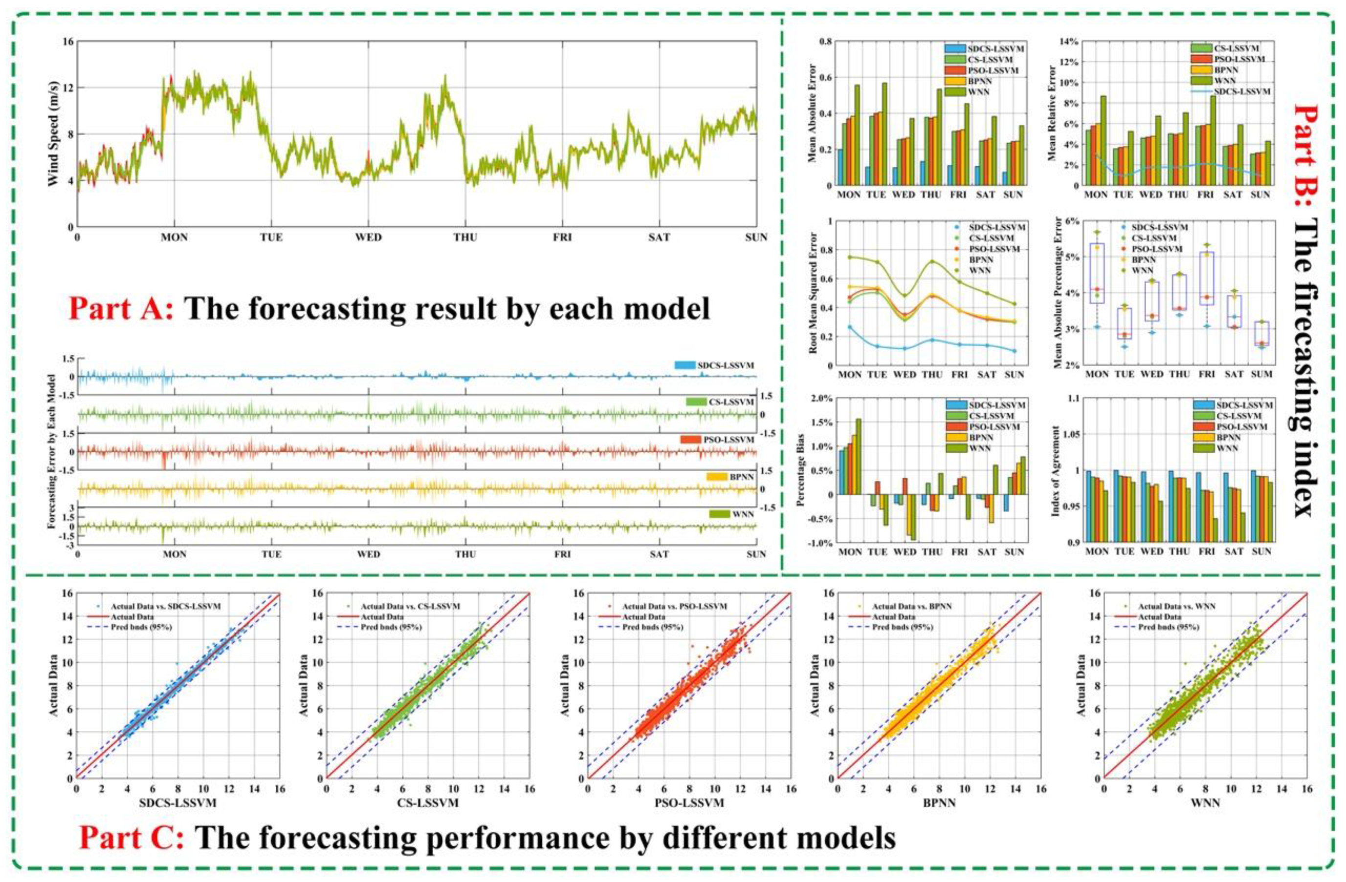
In particular, we use two-order forecast effectiveness in this paper. Moreover, two-order forecasting effectiveness of the proposed hybrid model is maximum from the following simulation results. From

Table 10. The two-order forecasting effectiveness of each model.

Observation Site	Model	Mon	Tue	Wed	Thu	Fri	Sat	Sun
Site 1	SDCS-LSSVM	0.93728	0.99108	0.98144	0.98225	0.97296	0.98165	0.99103
	CS-LSSVM	0.93602	0.97237	0.95323	0.95208	0.93796	0.95546	0.97017
	PSO-LSSVM	0.93507	0.97154	0.95033	0.95182	0.93769	0.95532	0.97004
	BPNN	0.90204	0.96106	0.93665	0.94113	0.90548	0.94247	0.95995
	WNN	0.89733	0.96099	0.93111	0.93217	0.90919	0.93549	0.95892
Site 2	SDCS-LSSVM	0.96861	0.99351	0.98199	0.98807	0.96918	0.98657	0.99668
	CS-LSSVM	0.94917	0.97304	0.96243	0.96867	0.94937	0.96665	0.97448
	PSO-LSSVM	0.94803	0.97260	0.96144	0.96829	0.94880	0.96609	0.97323
	BPNN	0.92801	0.96230	0.94756	0.94719	0.92681	0.95070	0.97027
	WNN	0.92458	0.96253	0.94292	0.94907	0.92423	0.94830	0.96771
Site 3	SDCS-LSSVM	0.99785	0.97858	0.97219	0.97681	0.95477	0.96794	0.98274
	CS-LSSVM	0.94618	0.96841	0.96221	0.96608	0.94526	0.95660	0.97234
	PSO-LSSVM	0.94522	0.96816	0.96200	0.96597	0.94485	0.95586	0.97225
	BPNN	0.92348	0.96090	0.95165	0.95268	0.92461	0.94503	0.96207
	WNN	0.91445	0.95864	0.94256	0.94908	0.91456	0.93977	0.96035
Site 4	SDCS-LSSVM	0.98917	0.96409	0.96305	0.96045	0.94512	0.97495	0.97464
	CS-LSSVM	0.93956	0.95199	0.95343	0.94888	0.93535	0.96523	0.96375
	PSO-LSSVM	0.93940	0.95193	0.95287	0.94788	0.93426	0.96489	0.96242
	BPNN	0.91808	0.94188	0.93166	0.92964	0.90260	0.95484	0.95169
	WNN	0.90952	0.94103	0.92540	0.92470	0.89879	0.94571	0.94558

we can clearly see that second-order forecasting effectiveness offered by the proposed hybrid model outperforms the other four models for wind speed forecasting at different sites. For example, for Site 1, second-order values of WPT-SDCS-LSSVM from Monday to Sunday are 0.93728, 0.99108, 0.98144, 0.98225, 0.97296, 0.98165, and 0.99103, respectively, which are larger than the other model.

Remark 4.

The results indicate that the proposed hybrid model is more valid than and significantly superior to the other models. Accordingly, the proposed model can satisfactorily approximate the observed actual wind speed time series.

5. Conclusions

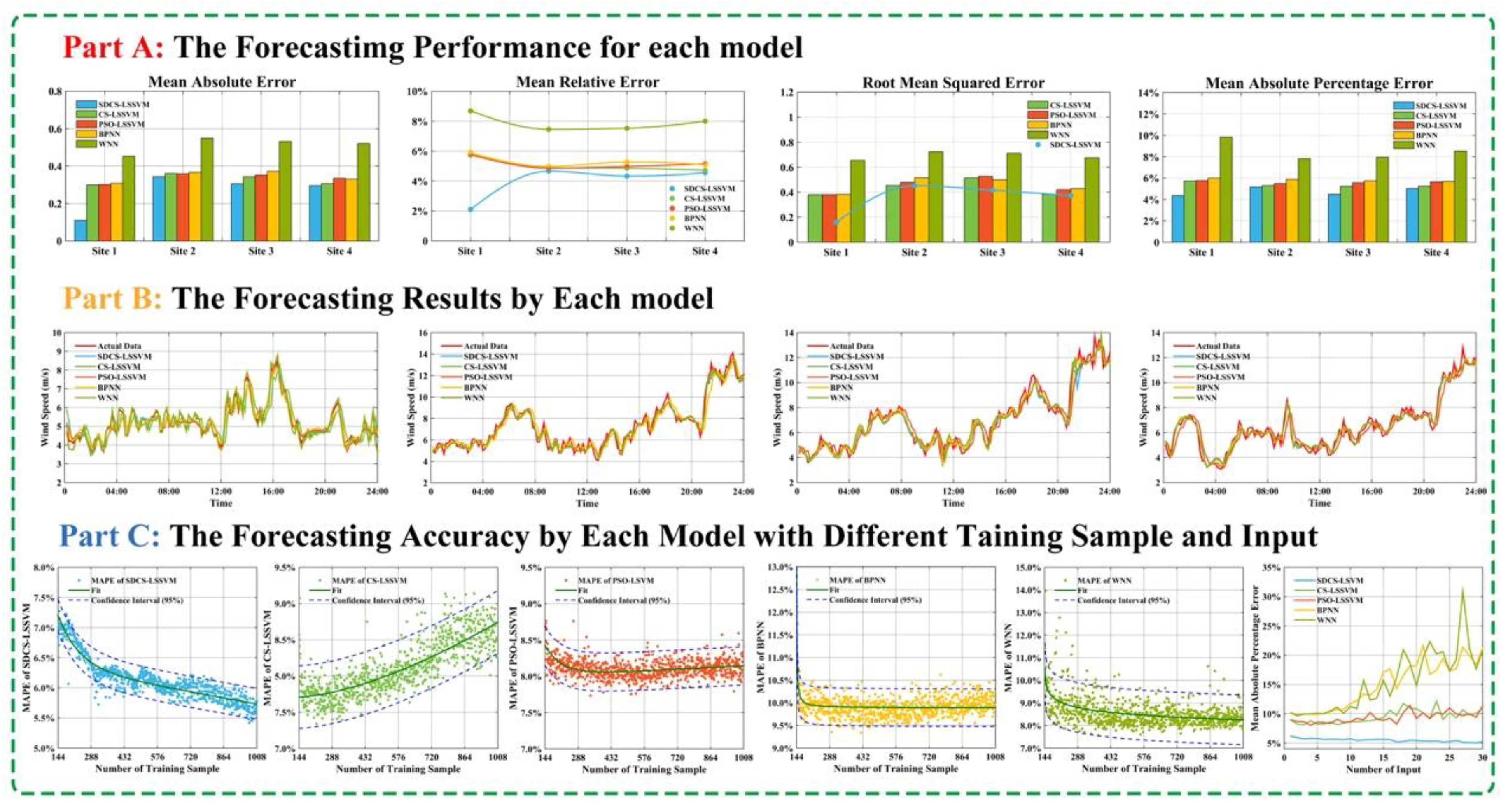
With the increasing utilization of renewable energy in recent years, wind energy is the largest new energy reserve, and the development and integration of wind energy resources into the power system are rapidly growing. It is noteworthy that both accuracy and stability should be regarded as equally vital in the forecasting field; thus, developing techniques to simultaneously achieve satisfactory accuracy and stability is imperative. However, because of the unique features of wind speed (uncertainty and intermittency), it is difficult to obtain satisfactory forecasting results using single models. To overcome this challenge, this research proposes a hybrid model based on an LS-SVM model that employs a modified cuckoo search algorithm to optimize the parameters of forecasting models for 10-min wind speed forecasting. Wavelet packet transform (WTP) in each WTP-ANN model is applied to denoise the wind speed series to improve the forecasting accuracy. Overall, for forecasting accuracy, the average MAPE values of WTP-BPNN, WTP-WNN, WPT-PSO-LSSVM, WPT-CS-LSSVM, and the hybrid model are 2.7565%, 3.0197%, 3.6897%, 3.0336%, and 1.5944%, respectively. Therefore, the proposed hybrid model can obtain satisfactory forecasting results for wind speed forecasting compared with the other four models. In addition, the fluctuations of MAPE values at each forecasting point are the smallest for the proposed hybrid model, which indicates that the model can improve the accuracy of wind speed forecasting. Moreover, the discussion of the hypothesis test and forecasting availability is used to evidence the superiority of the hybrid model compared to other models in this paper. As demonstrated by an instance based on a wind farm, the improvements in forecasting accuracy are significant for integrating electricity generated by wind energy into the grid with minimum risk and maximum benefit. The proposed hybrid model, which provides high forecasting accuracy, can be employed for wind farm dispatch and could improve the utilization of renewable energy.

References

1. Global Wind Statistics 2016. Available online: http://myemail.constantcontact.com/Release-of-Global-Wind-Statistics.html?soid=1102949362881&aid=jig4CtmWaNU (accessed on 10 February 2017).
2. Watts, J.; Huang, C. Winds of Change Blow through China as Spending on Renewable Energy Soars. The Guardian, 19 March 2012. [Google Scholar]
3. Chang, R.; Zhu, R.; Badger, M.; Hasager, C.B.; Xing, X.; Jiang, Y. Offshore Wind Resources Assessment from Multiple Satellite Data and WRF Modeling over South China Sea. Remote Sens. 2015, 7, 467–487. [Google Scholar] [CrossRef] [Green Version]
4. Dong, Y.; Wang, J.; Jiang, H.; Shi, X. Intelligent optimized wind resource assessment and wind turbines selection in Huitengxile of Inner Mongolia, China. Appl. Energy 2013, 109, 239–253. [Google Scholar] [CrossRef]
5. Mohammadi, K.; Alavi, O.; Mostafaeipour, A.; Goudarzi, N.; Jalilvand, M. Assessing different parameters estimation methods of Weibull distribution to compute wind power density. Energy Convers. Manag. 2016, 108, 322–335. [Google Scholar] [CrossRef]
6. Jiang, H.; Wang, J.; Wu, J.; Geng, W. Comparison of numerical methods and metaheuristic optimization algorithms for estimating parameters for wind energy potential assessment in low wind regions. Renew. Sustain. Energy Rev. 2017, 69, 1199–1217. [Google Scholar] [CrossRef]
7. Bowman, K.O.; Shenton, L.R. Estimation, Method of Moments [J]. In Encyclopedia of Statistical Sciences; John Wiley & Sons, Inc.: Hoboken, NJ, USA, 2004; pp. 252–261. [Google Scholar]
8. Aldrich, J.R.A. Fisher and the Making of Maximum Likelihood 1912–1922. Stat. Sci. 1997, 12, 162–176. [Google Scholar] [CrossRef]
9. Charnes, A.; Frome, E.L.; Yu, P.L. The Equivalence of Generalized Least Squares and Maximum Likelihood Estimates in the Exponential Family. J. Am. Stat. Assoc. 1976, 71, 169–171. [Google Scholar] [CrossRef]
10. Yang, X.S. Nature-Inspired Metaheuristic Algorithms; Luniver Press: London, UK, 2008. [Google Scholar]
11. Eiben, A.E.; Raué, P.E.; Ruttkay, Z. Genetic algorithms with multi-parent recombination. In Parallel Problem Solving from Nature—PPSN III, Proceedings of the International Conference on Evolutionary Computation—The Third Conference on Parallel Problem Solving from Nature Jerusalem, Israel, 9–14 October 1994; Springer: Berlin, Germany, 1994; Volume 866, pp. 78–87. [Google Scholar]
12. Waldner, J.B. Nanocomputers and Swarm Intelligence; Wiley-IEEE Press: New York, NY, USA, 2008. [Google Scholar]
13. Yang, X.S.; Deb, S. Cuckoo Search via Lévy flights. In Proceedings of the 2009 World Congress on Nature & Biologically Inspired Computing (NaBIC), Coimbatore, India, 9–11 December 2009; pp. 210–214. [Google Scholar]
14. Cassola, F.; Burlando, M. Wind speed and wind energy forecast through Kalman filtering of Numerical Weather Prediction model output. Appl. Energy 2012, 99, 154–166. [Google Scholar] [CrossRef]
15. Liu, H.; Erdem, E.; Shi, J. Comprehensive evaluation of ARMA–GARCH (-M) approaches for modeling the mean and volatility of wind speed. Appl. Energy 2011, 88, 724–732. [Google Scholar] [CrossRef]
16. Tascikaraoglu, A.; Uzunoglu, M. A review of combined approaches for prediction of short-term wind speed and power. Renew. Sustain. Energy Rev. 2014, 34, 243–254. [Google Scholar] [CrossRef]
17. Xiao, L.; Shao, W.; Yu, M.; Ma, J.; Jin, C. Research and application of a hybrid wavelet neural network model with the improved cuckoo search algorithm for electrical power system forecasting. Appl. Energy 2017, 198, 203–222. [Google Scholar] [CrossRef]
18. Yang, W.; Wang, J.; Wang, R. Research and application of a novel hybrid model based on data selection and artificial intelligence algorithm for short term load forecasting. Entropy 2017, 19, 52. [Google Scholar] [CrossRef]
19. Liu, H.; Tian, H.; Liang, X.; Li, Y. Wind speed forecasting approach using secondary decomposition algorithm and Elman neural networks. Appl. Energy 2015, 157, 183–194. [Google Scholar] [CrossRef]
20. Wang, J.; Du, P.; Niu, T.; Yang, W. A novel hybrid system based on a new proposed algorithm—Multi-Objective Whale Optimization Algorithm for wind speed forecasting. Appl. Energy 2017, 208, 344–360. [Google Scholar] [CrossRef]
21. Iversen, E.B.; Morales, J.M.; Møller, J.K.; Madsen, H. Short-term probabilistic forecasting of wind speed using stochastic differential equations. Int. J. Forecast. 2015, 32, 981–990. [Google Scholar] [CrossRef]
22. Carta, J.A.; Ramírez, P.; Bueno, C. A joint probability density function of wind speed and direction for wind energy analysis. Energy Convers. Manag. 2008, 49, 1309–1320. [Google Scholar] [CrossRef]
23. Oliveri, G.; Rocca, P.; Massa, A. Differential evolution as applied to electromagnetics: Advances, comparisons, and applications. IEEE Antennas Propag. Mag. 2011, 53, 3058–3059. [Google Scholar]
24. Golbon-Haghighi, M.H.; Saeidi-Manesh, H.; Zhang, G.; Zhang, Y. Pattern Synthesis for the Cylindrical Polarimetric Phased Array Radar (CPPAR). Prog. Electromagn. Res. 2018, 66, 87–98. [Google Scholar]
25. Best, R.W.B. The capacity factor of a wind turbine cluster. Wind Eng. 1981, 5, 235–241. [Google Scholar]
26. Daubechies, I. Ten lectures on wavelets. Comput. Phys. 1998, 6, 1671. [Google Scholar]
27. Suykens, J.A.K.; Van Gestel, T.; De Brabanter, J.; De Moor, B.; Vandewalle, J. Least Square Support Vector Machine. Euphytica 2002, 2, 1599–1604. [Google Scholar]
28. Myttenaere, A.D.; Golden, B.; Grand, B.L.; Rossi, F. Mean Absolute Percentage Error for regression models. Neurocomputing 2016, 192, 38–48. [Google Scholar] [CrossRef] [Green Version]
29. Wang, J.; Heng, J.; Xiao, L.; Wang, C. Research and application of a combined model based on multi-objective optimization for multi-step ahead wind speed forecasting. Energy 2017, 125, 591–613. [Google Scholar] [CrossRef]
30. Jiang, Y.; Song, Z.; Kusiak, A. Very short-term wind speed forecasting with Bayesian structural break model. Renew. Energy 2013, 50, 637–647. [Google Scholar] [CrossRef]
31. Jolayemi, E.T. A Multiraters Agreement Index for Ordinal Classification. Biom. J. 2010, 33, 485–492. [Google Scholar] [CrossRef]
32. Khalid, M.; Savkin, A.V. Adaptive filtering based short-term wind power prediction with multiple observation points. In Proceedings of the 2009 IEEE International Conference on Control and Automation, Christchurch, New Zealand, 9–11 December 2009; pp. 1547–1552. [Google Scholar]
33. Hu, Q.; Zhang, S.; Xie, Z.; Mi, J.; Wan, J. Noise model based ν-support vector regression with its application to short-term wind speed forecasting. Neural Netw. 2014, 57, 1–11. [Google Scholar] [CrossRef] [PubMed]
34. Bivona, S.; Bonanno, G.; Burlon, R.; Gurrera, D.; Leone, C. Stochastic models for wind speed forecasting. Energy Convers. Manag. 2011, 52, 1157–1165. [Google Scholar] [CrossRef]
Figure 1. Flowchart of wind speed forecasting. (First step: wavelet packet transform is used to deal with the original wind speed time series; the wavelet function is Daubechies (db) and decomposition level is 7. Second step: preprocessing wind speed time series is divided into training and testing, the number of training samples is set at 1008 and testing samples at 144. Third step: the modified cuckoo search algorithm with steepest descent (SDCS) algorithm is used to optimize the two hyperparameters: regularization (Gam) and tuning parameter (Sig2) of LSSVM and the parameters of artificial neural network (ANN) models. Fourth step: output the forecasting values by each model and compare the performance.
Sustainability 10 03913 g001
Figure 2. The analysis of wind energy resources distribution.
Sustainability 10 03913 g002
Figure 3. Relationship between input and training sample.
Sustainability 10 03913 g003
Figure 4. Weekly forecasting performance of each model in Site 1.
Sustainability 10 03913 g004
Figure 5. A weekly forecasting result of each model in Site 2.
Sustainability 10 03913 g005
Figure 6. A weekly forecasting result of each model in Site 3.
Sustainability 10 03913 g006
Figure 7. A weekly forecasting result of each model in Site 4.
Sustainability 10 03913 g007