Strategic Cross-Border Water Pollution in Songliao Basin

1
School of Business Administration, Northeastern University, Shenyang 110169, China
2
Jangho Architecture College, Northeastern University, Shenyang 110169, China
*
Author to whom correspondence should be addressed.
Sustainability 2018, 10(12), 4713; https://0-doi-org.brum.beds.ac.uk/10.3390/su10124713
Submission received: 17 October 2018
/
Revised: 6 December 2018
/
Accepted: 6 December 2018
/
Published: 11 December 2018
(This article belongs to the Special Issue Regions and Economic Resilience)
Abstract
:This paper studies the two-fold impacts of environment regulation related to local officer promotion and water quality assessment of cross-border sections within the framework of the 11th Five-Year Plan. We employ the difference-in-difference (DID) and difference-in-difference-in-difference (DDD) models to a unique dataset on water polluting activities in Songliao Basin counties from 2003 to 2009. Empirical results show that on one hand, regulation and water pollution are negatively correlated, the stricter the regulation is, the less water pollution happens. On the other hand, as no explicit accountability and synergetic governance system were set up by the 11th Five-Year Plan, prefecture-level municipal governments tend to exert the least enforcement efforts in the most downstream counties. We find the evidence of strategic water polluting that the overall output value, new entry into and old business water polluting industries are significantly higher in the most downstream county of a prefecture-level city, relative to other similar counties.
1. Introduction
Cross-border water pollution refers to the pollution transferred from upstream to downstream jurisdictions by water flow. Such pollution has strong negative externality as shown by the phenomenon “one point polluted, the whole drainage basin affected” [1]. Due to the Songhua River and Liao River systems, Northeast China suffers from severe cross-border water pollution. The Liaohe River basin is highly industrialized. The industrial structure is composed of processing of agricultural products and byproducts, papermaking, fuel manufacturing, pharmaceutical manufacturing, and nonferrous metal smelting and rolling, all of which contribute to 81.6% of the total COD emissions [2]. In 2005, an explosion in a benzene factory of Jilin Petrochemical Corporation severely polluted the downstream cities of Songhua River including Changchun and Harbin [3]. The central government was shocked by the explosion event, which then explicitly addressed the water pollution challenge by specifying in the 11th Five-Year (2006–2010) Plan quantitative emission reduction targets for chemical oxygen demand (COD). More polluted regions were subject to higher COD reduction targets. The government also set up a monitoring system on cross-border river quality and linked local officials’ promotion with these targets for the first time [4,5,6]. Local officials who failed to the pollution reduction mandates would be removed from office.
Songhua River and Liaohe River both belong to the Northeast geographical unit. They have similar natural characteristics and economic situation which play various important roles in transportation, tourism, irrigation, and so on. The most important is that they are the main source of drinking water for Northeast China. As the main agriculture drainage basin in China, the two rivers both run through major coal, steel, petrochemical, and equipment manufacturing industry hubs [1,2,7,8]. Compared with the other five major rivers in China, rivers in the Northeast have significant inherent characteristics: freezing of the water surface in winter and a long dry season and having many tributaries (both big and small) with small water flow. As a result, both rivers have poor self-purification capacity and are more vulnerable to border pollution. As of 2017, the central government set up 33 water quality monitoring stations along prefecture borders in Songhua River and Liaohe River to solve the cross-border water pollution problems in Northeast China. The data from these stations show that the water quality of Songliao Basin has had little improvement in recent years.
On the other hand, the pollution prevention and treatment monitoring system in China is relatively decentralized. The central Bureau of Environmental Protection (BEP) formulates the overall environmental goals and monitors enforcement activities of local BEPs. All regional level (province, prefecture, and county) BEPs formulate local environmental regulations as well as monitor the permit systems which require that all industrial projects obtain approval from the local BEPs before production to ensure that new projects meet the basic environmental standards. Regional works are governed by superior environmental authorities while they administratively belong to the government at the same level and are also subject to the strategic development goal of the local government. Disparities between the economic development and the environmental goals of local government have always led to the lax regulatory and in a lower standard of monitoring and enforcement duties to support a “pollution-friendly” investment and business environment [9,10]. Though the cross-border river cross-section assessment system is listed in the 11th Five-year Plan, no explicit accountability or synergetic governance system was set up. Under the pressure from the central government to curb water pollution, growth-driven local governments responded by optimally allocating enforcement efforts among their counties: given geographical differences and the externalities inherent in water pollution, the local government cannot reap the full benefits of pollution reduction in the downstream area of their jurisdiction. Meanwhile, the central government gives the local government considerable power over the enforcement of environmental regulations. Therefore, local government tends to ignore the monitoring of the most downstream counties.
Based on previous studies and current scenario in China, this paper infers that the impact of the 11th Five-year Plan’s environmental policies amendment on Northeast China has been two-fold: on one hand, local officers try to control pollution in their regions and lower risks for such promotion, on the other hand, the system structure, especially the non-cooperative mechanism and monitoring technology, drives prefecture-level municipal governments to have much laxer environmental regulations in the most downstream county (district) which attracts more water polluting activities. By transferring negative externalities (pollution) to adjacent downstream regions, the local government can meet both the economic development goals and reduction requirements mandated by the central government.
This paper provides a scientific basis for decision-making on industrial water pollution control in Northeast China and breaks the assessment mechanism of “bottom line competition” in prefecture-level cities, to achieve the goal of sustainable development.
2. Literature Review
Many studies have analyzed the cross-border water pollution situation after decentralization of authority between the central and local governments from a theoretical perspective. They have concluded that conflicts between interest groups affect the synergy and governance efficiency, resulting in the discharge reduction goal remaining unfulfilled [11,12,13]. H Sigman used water pollution data from 500 monitoring stations to explore the evidence, which indicated the fact that in the United States, decentralized environment governance in various states caused the spillover of cross-border river pollution, based on which he consequently drew the conclusion that the United States’ environment governance decentralization is cost-effective [1,14]. Zeng Wenhui set up an “equalized pollution” model to analyze the motivation of “hitchhiking” activities in upstream regions; this model revealed that the geographic location of provinces has a strong impact on environmental regulations [15]. ME Kahn used data from the main monitoring stations of seven major rivers during 2004 to 2009 and found that after the 11th Five-year Plan linked officer promotion opportunities with water pollution indexes, the COD content reduced faster in provincial boundary stations than in other inland stations; while there is no significant improvement in other sources of water pollution alongside the boundaries [6]. Hu Zhenyun set up a game model on government and enterprise water pollution treatment and found that as the central government calls for ecological civil engineering development, the environmental performance of local government improves and overall corporate emissions are reduced [16]. Jie He [17] assessed payment willingness for cross-border water pollution treatment of 20 cities in Xijiang River Basin; the result showed that upstream regions are relatively unwilling to pay for pollution costs while the willingness of the downstream to pay costs negatively correlates with the upstream pollution levels.
As far as regional socioeconomic development and water pollution problems concerned, the spatial awareness of the government with respect to its strategic decision-making is extremely important. Molly Lipscomb used visual functions of ArcGIS to collect lighting data of river monitoring stations and found that water polluting enterprises, guided by local government strategies, moved to upstream places of the rivers [18]. Zhang Shanshan [19], using the kernel density estimation to study the spatial characteristics of enterprise movement in the Taihu Basin, found that after the establishment of local water environmental regulations, many enterprises moved from upstream to the outskirts or even to places far from rivers and lakes. Zhao Guohao [20] set up a Spatial Autoregressive Model based on data of 285 prefecture-level cities during the period of 2003 to 2015 and concluded that implementation effects vary in different regions; the “bottom competition” was driven by eastern regional governments pushing polluting enterprises to move towards the central and western regions. Haoyi Wu used the Logit Model to study the impact of the 11th Five-year Plan environment policy on new water polluting enterprises, the result of the study showed that the environmental incentive mechanism lacks reasonability as it pushes new polluting enterprises to select sites in central and western regions—the “polluting paradise”—rather than the eastern or coastal regions, and such actions would deteriorate national water pollution throughout the downstream as water sources of the Yangtze River and Yellow River are both located in the western regions [21]. Shi Minjun set up a spatial estimation methodology to calculate COD emission per province per industry and found that during the 11th Five-year Plan period, the development of papermaking and paper products industry in the western regions contributed the most to pollution reduction, while those in central regions contributed the least [22]. Zhao Chen utilized the Distance Distribution Dynamics model to study spatial changes of enterprise activity caused by the environment regulation, and the spatial difference between the upstream and downstream of Yangtze River Basin after the 11th Five-year Plan and found evidence of the industrial transfer in China [23]. Hongbin Cai studied 24 rivers in China and found that after the decentralization due to the 11th Five-year Plan, local environments relaxed their regulations on the most downstream regions, to transfer negative externality caused by pollution, thereby making water polluting activities in such places more frequent [24].
From the above, scholars tend to focus on the following aspects of cross-border water pollution problems.
(1) The process of negotiation and mutual restraint amongst intra-authoritative entities (include central government, local governments, environmental departments, and so on) after decentralization had dramatically reduced the management efficiency in upstream regions. Studies rely on theoretical studies or quantitative research of enterprises and government spatial strategies from a visual perspective, and mostly lack empirical literature.
(2) Some of the existing literature focuses on the four major economic zones, while others focus on the provincial scale or traditional upstream and downstream perspectives. However, most of them ignore the importance of smaller scale, especially the upstream/downstream counties at prefecture-level borders. (a) A study at such a large scale ignores details of many economic activities and makes the results biased. (b) Regions alongside the provincial boundary are rarely economic hubs, due to their small economic volume and low pollution scales, and thus such places could not represent the holistic water pollution scenario. (c) China’s “Key Points of Regional Planning” stipulates that all administrative entities above county level shall be responsible for the real-time water quality monitoring. The prefecture government entities are directly accountable for their corresponding watershed pollution. Administration department of county level of at higher levels shall be responsible for the dynamic monitoring of water sources. The prefecture is the basic administrative unit for water pollution accountability; as such, counties (districts) in conjunction with prefecture-level city borders are the best research objects for this purpose.
(3) Most scholars use monitoring station cross-section data as water pollution indexes, however, this data reflects the aggregation of both local and upstream pollution, which will not provide accurate description for local water pollution. Moreover, monitoring stations were randomly located, and do not cover all the administrative borders in northeast China.
(4) After the 11th Five-year Plan, the central government strategically re-allocated polluting enterprises to achieve the goals of economic growth and environment protection by enforcing stronger pollution control policy. Accordingly, enterprises reacted to the regulations as well. While research the strategic allocation of enterprises based on governmental policies, previous study did not verify the relationship between the intensity of environmental regulation and water polluting enterprise activities.
This paper is however based on the concept of cross-border water pollution. Using water polluting enterprise activities as a substitute for monitoring data, we employ an optimal assessment model to systematically analyze the allocating of pollution activities between counties by prefecture-level governments within the framework of the 11th Five-Year Plan.
First, we focus on the cross-border water pollution at the prefecture-level basis, rather than the economic zone or traditional upstream/downstream (divided by a point in the drainage basin) basis.
Second, we take microenterprises production activities (total industrial output value and quantity of new/old enterprises) as substitute variables for water pollution indexes to determine the point sources for local pollution.
Third, we first verify the relationship of regulation and water polluting activities in the context of the different environment policies stipulated by the 11th Five-year Plan, and then, study the spatial differences of regulation in conjunction with the river, to further assess the government strategy allocating water polluting enterprises.
Fourth, we not only focus on water pollution activities of counties on the borders, but also take into account water polluting activities of nonborder riverside counties to achieve a more realistic outcome.
3. Materials and Methods
3.1. Sample Introduction
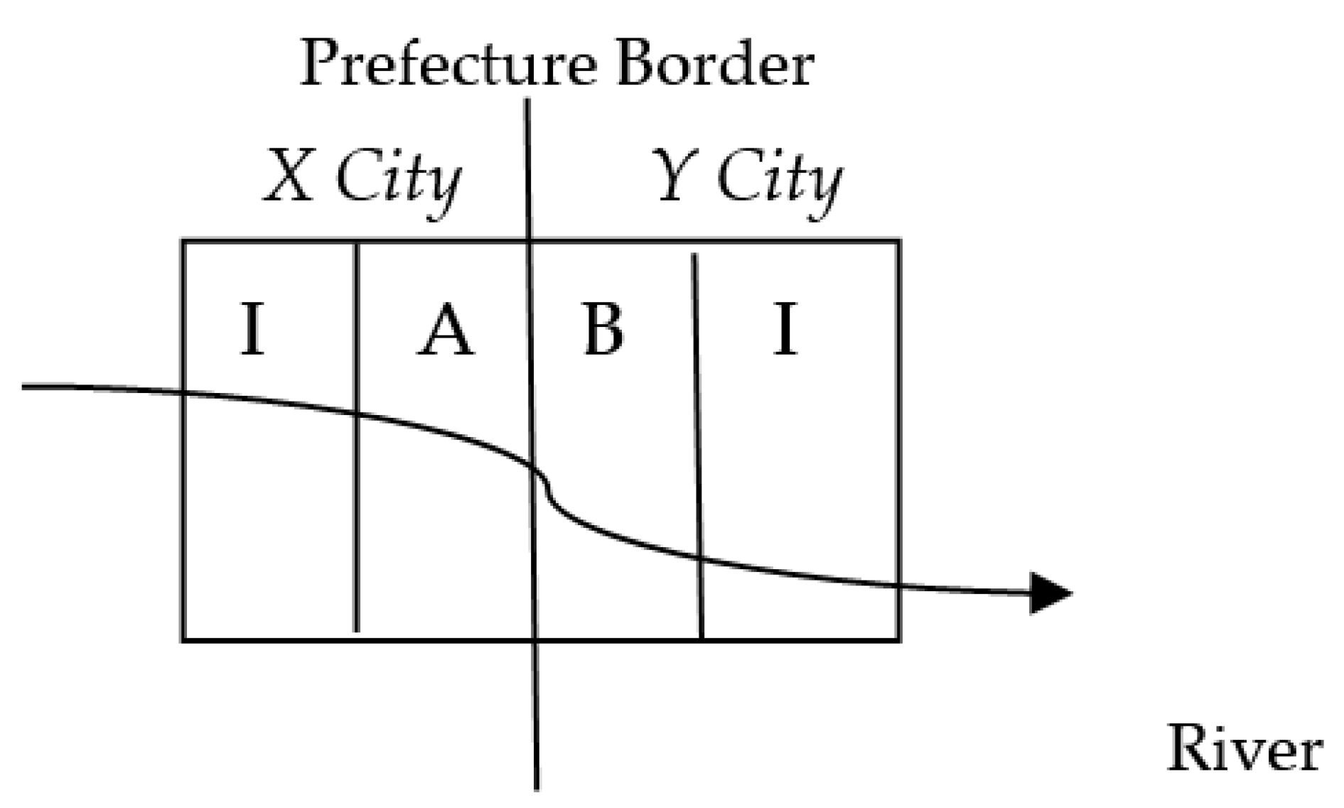
We expect to see rising levels of water pollution in the most downstream county of a prefecture-level city, as a result of the prefecture-level municipal governments’ mandates, since the rivers flows through the city and there are multiple districts (the same administrative level to counties) in a city. Thus, this research refers to the samples from districts and counties as being the same, and considers them as county samples. To illustrate our empirical strategy, we design the Figure 1. As non-riverside regions are not directly affected by river pollution, we only focus on type-A, type-B, and type-I counties along the rivers.
3.2. Empirical Design
The main purpose of the empirical analysis is to identify the effect of environmental policy on local industrial production activities. Therefore, we can verify the relationship of regulation and water polluting activities in the context of the different environment policies stipulated by the 11th Five-year Plan. Then, by comparing differences of industrial production activities in type-A, type-B, and type-I counties, we can identify the cross-border pollution brought by spatial strategy of prefecture-level municipal government.
According our empirical design, Hypothesis 1 verifies the relationship of regulation intensity and water polluting activities (overall output value is the proxy variable). The expected results are negatively correlated. In Hypothesis 2, we empirically test that type-A county has the most water pollution activities. Therefore, the environmental regulation of type-A county is more relaxed than type-B and type-I counties. By the above argument we find the evidence of strategic pollution by prefecture municipal government (see DID analysis).
In the DDD analysis section, first we compare the effects of environmental regulations in seven water pollution industries. Then we empirically examine the changes in the number of new and old enterprises in type-A, type-B, and type-I counties. This will provide evidence that the prefecture-level municipal governments strategically reduce the enforcement of environmental protection in their administrative region.
3.2.1. Differences-in-Differences Method (DID) Model Setting
To observe impact brought about by the 11th Five-year Plan water pollution regulation, this paper uses a globally universal policy assessment method: Differences-in-Differences Method (DID) [25,26,27]. Its basic thought is to simulate natural experiment, divide observing objects into a control group (not affected by policies) and treatment group (affected by policies), and then compare changes of the two groups before and after the implementation of policies to assess their real policy effects. If changes of the treatment group are significantly greater than those in the control group, it indicates that the policy effect is remarkable; otherwise the policy effect is unremarkable.
Before 2006, the central government documents did not provide for the linking of pollution reduction targets with the officer promotion incentive system. In August of the same year, the BEP and the National Development and Reform Commission announced an overall control plan for COD during the period of the 11th Five-year Plan (2006–2010), correlating government officer assessment and promotion with the environmental protection target [28,29,30]. We posit that water pollution activities in locations with stringent regulations would decrease more than in locations with relatively lax regulations after 2006. However, before 2006, regulation stringency was almost uniform across counties. This is a standard DID exercise, where the production activities of water-polluting enterprises before 2006 are the control group.
Hypothesis 1.
Regulation strength is inversely correlated to water polluting activities.
The DID basic econometric model is presented as follows
indicates the production activities of water polluting industries in county c during the year t; refers to regulation strength of county c, indicating the implementation of environmental polices of different counties after the 11th Five-year Plan; and Postt is the visual variable of treatment period, for ∀t ≥ 2006, , otherwise . Rc × Postt is the interaction term of policy regulation and time visual variable, coefficient (differences-in-differences estimator) measures the effect of policy which can show the regulation effects; a negative value indicates that government regulation strength is inversely correlated to enterprise activities, while a positive value indicates otherwise. and are essential fixed constituent parts of model setting, the former represents the fixed effect of counties, capturing time-invariant characteristics (such as weather, geographic features, natural resources, etc.), belonging to region c; the latter represents the annul fixed effect, capturing annul factors that have the same impact on all counties (such as macroeconomic fluctuation, business cycle, financial & monetary policies, etc.); and is the random error term.
is the annul dummy variable; for given years its value is set as 1, otherwise = 0. β04 ~ β09 are its corresponding coefficients to observe water polluting production activity fluctuation over time; a positive value of these coefficients indicates growing industrial activities in that year, while a negative value indicates otherwise; the 11th Five-year Plan came into force in 2006; limited by the data availability, samples are chosen from 2003 to 2009. Taking the year 2003 as base period to analyze water polluting activity trend during 2004 to 2009; represents error items that could hardly be observed by measurement methods.
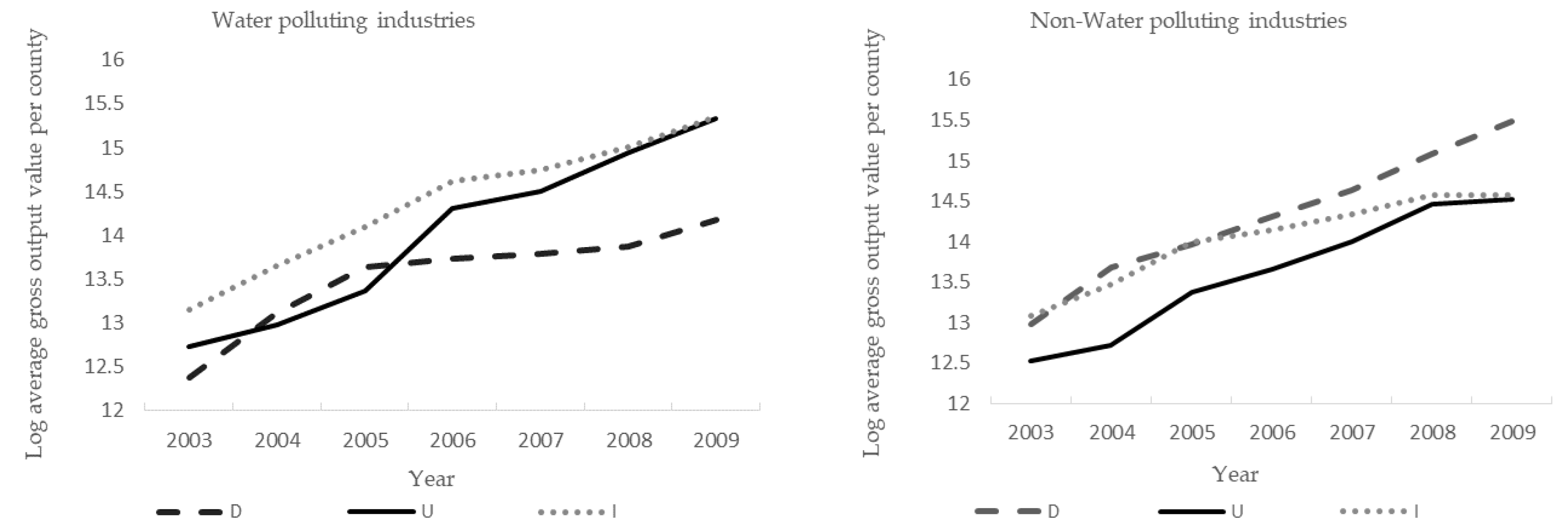
By comparing differences of water polluting activities (output value, numbers of new and old enterprises) in different locations of a river, we can find the evidence of the downstream effect. As shown in Figure 3, after 2006, compared to the other two type counties (B and I), the output value of water polluting industries grew faster in type-A counties. The statistical results provide an opportunity for implementing a difference-in-difference (DID) strategy. Specifically, water polluting industries in type-A counties are treatment groups, while water polluting production activity in type-B and type-I counties are control groups.
From this, we propose Hypothesis 2:
Hypothesis 2.
Within the entire Songliao basin, the type-A county is the most laxly regulated region which attracts more water polluting activities.
The DID basic model is presented as follows
is the county type. It is set as 1 if county c is the type-A county, represents visual variable before and after the treatment, for , , otherwise . Only after 2006, the value of type-A counties interaction term is set as 1. Positive value of factor indicates that after 2006, compared to type-I and type-B counties, water polluting activities in type-A counties grew faster; negative value of factor indicates the opposite; and dependent variable have the same meaning as the above.
3.2.2. DDD (Differences-in-Differences-in-Differences) Model Setting
The problem of DID estimation method may correlate some time-varying county characteristics with and bias the estimation of . County factors including aggregation effect, input–output of transaction parties in a vertical industrial chain, and labor market efficiency, might change with time and cause deviation in the value; hence, it is hard for models (1) and (2) to cover all the influence factors.
To overcome this problem, factors listed below should be taken into consideration: there is regulation effect on heterogeneity between water polluting and nonwater polluting industries, taking the latter as control group and the former as treatment group to set up the DDD estimation model:
We construct a balanced panel data set; each observation represents the situation in a two-digit industry in a county in a year. represents the production activities of i industry in c county in the year t; Dirtyi indicates the industry nature, if industry i is water polluting, = 1, otherwise = 0. The major advantage of the DDD model is that it allows us to include the county-year fixed effect which not only controls time-varying and time-invariant county characteristics (such as producing technology spillover, local public policies, labor quality, etc.) that could not be controlled by the DID model. Moreover, the DDD model also covers industry-year fixed effects that capture all time-varying and time-invariant industrial characteristics, such as specific industrial technologies and government industrial policies. Furthermore, we include industry–county fixed effect to allow production activities to differ across counties. represents error items that are hard to observe or measure by econometric method, error items of different periods in the same industry (county) may be serially correlated, and such potential spatial and time serial correlation should be controlled by using county and industrial two-way robust standard errors. In DDD model (3), by controlling factors that may affect policy effects, biased estimation of caused by factors other than policies (namely the industry changing over time and the industry changing over counties, which are time-related) is avoided, to get the most accurate value representing the policy effect. The focus of our DDD analysis is the triple interaction term , so is the parameter of primary interest to us which measures the pure effect of policy. A negative value of indicates that the 11th Five-year Plan water polluting regulations are inversely correlated with water polluting industrial production activities—the stricter the regulation is, the faster the production activities diminished. On the contrary, a positive value of indicates that the 11th Five-year Plan water polluting regulations are positively correlated with water polluting industrial production activities—the stricter the regulations are, the faster the production activities grow.
3.3. Variable Selection and Data Sources
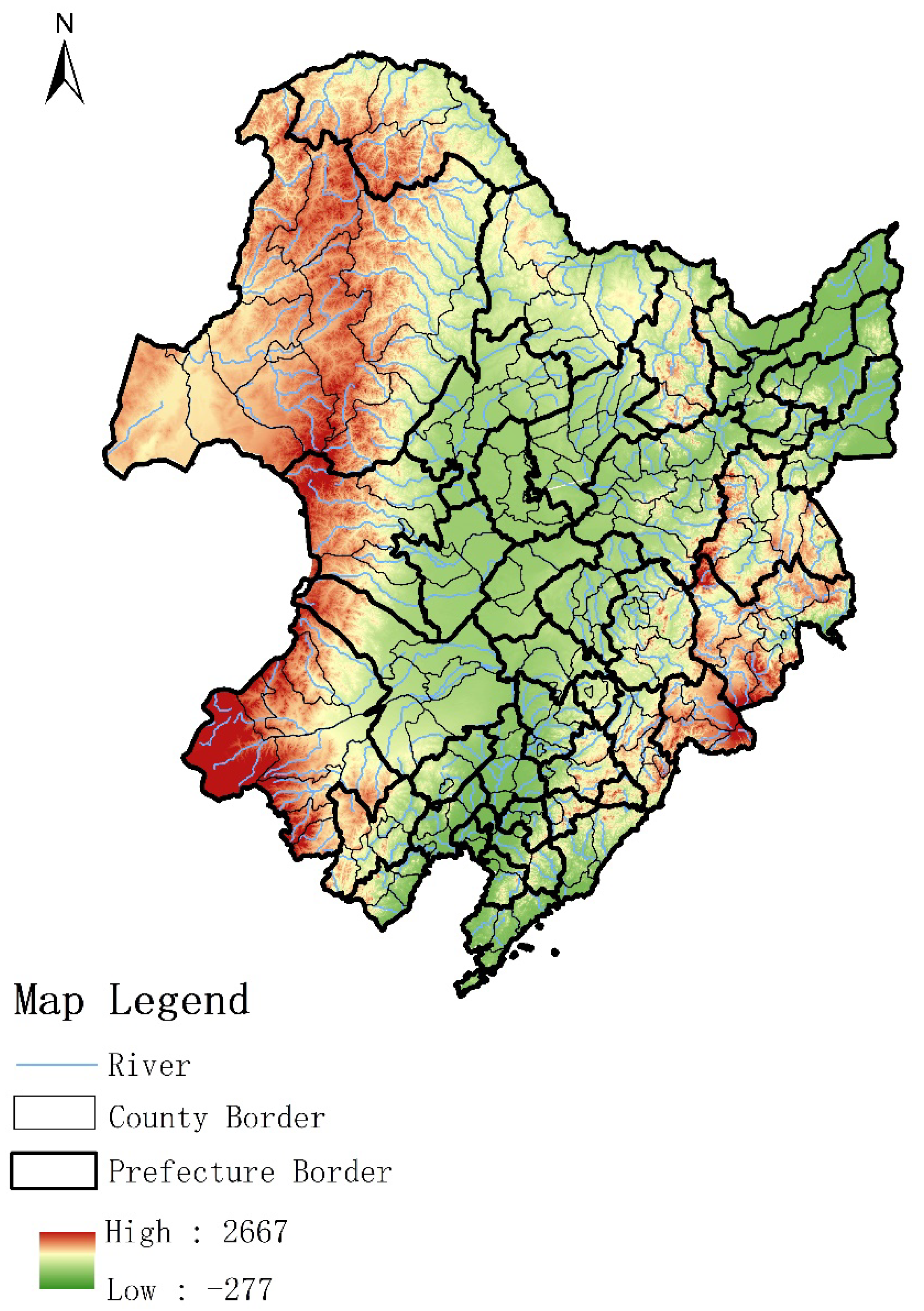
We focus on the main streams and tributaries of Songhua River and Liao River in northeast China, each of which cross at least one prefecture-level city border. In the Songliao Basin, we first identify 168 riverside counties (such as counties A and B) located at prefecture-level city borders. Then we identify 49 riverside counties (such as counties I) that are not located at prefecture borders. Our final sample has 217 counties in total, of which there are 84 type-A counties, 84 type-B counties, and 49 type-I counties. While the 11th Five-year Plan came into force in 2006, we construct a sample with data ranging from 2003 to 2008.
3.3.1. Water Pollution Regulation Index
Water polluting regulation is always multidimensional and complex [31,32]; environmental departments of various regional (province, prefecture, and county) level governments are responsible for formulating and implementing local environmental regulations. Generally, they use preproject license and postproject punishment as managerial measures. License system stipulates that all industrial projects must get permission before production begins from local environmental authorities, to ensure that the new projects conform to applicable standards. Postproject punishments include warnings, revoking of business licenses, lawsuits, etc. Many scholars use postproject measures, which when compared with preproject ones directly aim at pollution, with easy to acquire postproject data; yet enterprises may react fiercely against such punishments with some under the table counter-measure, which constantly and dramatically reduce the punishment efforts.
a. The County-Level COD Reduction Mandate
Generally speaking, the environmental regulations are stricter in developed regions where polluting industries play important roles. In the 11th Five-year Plan, the central government’s water pollution criteria only targeted COD emissions. Therefore, this paper only considers the COD index. According to realistic experiences and research demands, we adapt COD emission reduction target distribution formula by China SEPA in 2006 to estimate the pre-operational water pollution regulation stringency of each county.
Original formula:
Bringing in economy proportions and industrial structure factors of the counties:
emission reduction target data of the provinces are from China SEPA: Using the study results of Wu Haoyi for reference, is the weight which represents each industry’s proportion of total industrial COD emission[21]; yic and yip represent output value of enterprises from i industry in various riverside counties and such value from i industry in each province p, respectively, and this data comes from China Industry Business Performance Data.
b. The Environment-Related Text Proportion of Each County’s Government Report
Measures of water polluting substances include COD, as well as levels of permanganate, ammonia, nitrogen, etc. Environmental efforts of local governments are not confined to just COD reduction, as a consequence. We developed an alternative stringency measure based on each county’s government report to measure the government’s desire to reduce pollution. Under pressure from superior government and local citizens, regional governments have to talk about environment issues in the annual work report. The government work report has an important role in local government documents; it covers accomplishments and problems regarding aspects including economic development, living standards of residents, import and export, environment protection, etc., of the previous year; it also involves setting up detailed goals for the next year. As government work reports are based on accurate statistical data and could reflect local work focus, thus the textual proportion regarding specific policies are usually taken to measure regional officers’ efforts on expected goals [33]. This document takes the proportion of environment-related text (including environment, power consumption, emission reduction, environment protection, ecology, pollution discharge, etc.) in regional government work reports as the substitute variable for environment regulation. Government work reports from 2003 to 2009 were taken from the Internet with only 132 counties (districts) available, of which 62 are type-A counties, 46 are type-B counties, and are 24 type-I counties.
3.3.2. Enterprise Production Activity Indexes
We take overall output value and the numbers of new and old enterprises of water polluting and nonwater polluting enterprises in 2003–2009 as proxy variables for enterprise activities. According to the “Classifying Standard of Water Polluting Industries” announced by the Ministry of Environmental Protection in 2010, the seven polluting industries are agricultural product and byproduct processing, textile manufacturing, clothing manufacturing, papermaking, petrochemical fuel manufacturing, chemical engineering, and nonferrous metal smelting; other industries are all classified as nonwater polluting ones [34,35]. The data comes from China Industry Business Performance Database which discloses basic information—such as assets and liabilities, industrial product revenue, operating status, and so on—of enterprises above designated size. We take advantage of microenterprise-level as well as industry-level data to give microdata support to study polluting enterprise activities in Northeast China (four provinces and regions) and to find polluting point sources [36].
The descriptive statistics of aforesaid variables is shown in Table 1.
4. Results and Discussion
4.1. DID
4.1.1. Identifying the Relationship between Regulation and Polluting Activities (Assumption 1)
By observing the regression results of DID in Table 2, the results indicate that when taking all samples as a whole—the estimated results in columns (1) and (2)—the coefficients of interaction items are all negative and significant, indicating that intensity of regulation is negatively correlated with water polluting enterprise activities. Water pollution activities in locations with stringent regulations decrease more than in locations with relatively lax regulations. Thus, the empirical results accord with the anticipated values and indicate the pollution reduction effects of the environmental policies of the 11th Five-year Plan. All annual dummy variable coefficients are positive and continuously growing, demonstrating that water polluting activities in Songliao basin are growing and expanding annually.
4.1.2. Identification of Strategic Allocating Polluting Activities by Prefecture-Level Municipal Government (Assumption 2)
In the estimated results of column (3), the interaction item coefficient is positive and significant. Based on Figure 3, the model clearly shows that “strategic pollution” plays an important role even though there may exist many uncontrolled complex factors that affect the result. Water pollution production activity increased more in the most downstream county (type-A counties) in a prefecture-level city after 2006. In the above, we prove that the intensity of regulation is negatively related to polluting activities, showing a relatively laxer water pollution regulation in the most downstream county (type-A counties) in a prefecture-level city than that in the two other counties. In column (4), for nonwater polluting industries, we do not find a significant increase in type-A counties relative to the other two counties. The positive externality of good water quality cannot be shared by all other areas of a prefecture-level city. Therefore, governments deliberately arrange polluting activities in the most downstream county to acquire the economic benefits of their administrative jurisdiction, and unilaterally transfer negative polluting externality to downstream regions, while assuring that the monitoring station data are able to meet discharge reduction requirements set by the central government. The concentration of water polluting activities in type-A counties provides solid evidence for demonstrating strategic allocating by prefecture-level Municipal government.
4.2. DDD
4.2.1. Identifying the Relationship between Regulation and Polluting Activities
The DDD model could solve the potential endogenous problem caused by omitted time-varying county characteristics; the first 2 columns of Table 3 show the regression results with COD discharge as the regulation measure. The 1st column shows the average impact of regulation on the selected water polluting industry; the triple interaction coefficient is negative and significant. The intensity of regulation is negatively correlated with water polluting enterprise activities corresponding to columns (1) and (2) of DID in Table 2. To test regulation effect of each water polluting industry, in column (2), the average impact of regulation policies on seven water polluting industries (agricultural product and byproduct processing, textile manufacturing, clothing manufacturing, papermaking, petrochemical fuel manufacturing, chemical engineering, and nonferrous metal smelting) are respectively shown, indicating negative and significant regulation effect that corresponds to overall triple interaction coefficient value. The intensity of regulations is ranked as follows (from strong to weak), textile manufacturing, clothing manufacturing, nonferrous metals smelting, agricultural products and byproduct processing, chemical engineering, petrochemical fuel manufacturing, and papermaking.
The regression results of taking the environment-related text proportion in the government work report as regulation measures are shown as column (3) and (4), the coefficients are still negative and statistically significant with similar results as the first two columns, indicating the former selection of the regulation variable is correct.
4.2.2. Spatial Transfer of Water Polluting Activities
DID results show that after the execution of 11th Five-year Plan came into force in 2006, the overall regulation improved; prefecture-level municipal governments strategically lowered the environmental protection strength in the most downstream counties within their administrative regions. The pollution regulation in type-A counties is not as strict as that of other regions, and water polluting enterprises react to such differences according to their own interests. Thus, we need to clarify the overall factors that may affect water polluting enterprise location and production selection, based on which we can assume that regulated by central government’s environmental policies, old water polluting enterprises weigh the costs–benefits and transfer their business from type-I and type-B counties to type-A counties, while new water polluting enterprises set up their factories in the most downstream counties of prefecture-level cities. In this section, we use spatial transfer of new/old water polluting enterprise into/out of various locations of rivers to verify the strategic allocating of the prefecture-level municipal government. Based on previous experiments, the year 2000 has been taken as a dividing point for new and old enterprises for their establishment information index selection so as to calculate the number of new/old riverside enterprises. DDD setting of model (3) is to test the response of new/old water polluting riverside enterprises to regulation policies.
The coefficients of column (1) and (4) in Table 4 are significantly positive, indicating that after the 11th Five-year Plan announced the environmental policy adjustment, and as regulations in various riverside regions got stricter, the number of new polluting enterprises in type-A counties increased. Coefficients in columns (2), (3), (5), and (6) are significantly negative, and the absolute values of coefficient in type-I counties are smaller than those in type-B counties, indicating that as water polluting regulation got stricter, production activities by new polluting enterprises in type-I and type-B counties decreased; while within the same prefecture-level city, county B is located upstream of the river in county I. To prevent upstream pollution, lower the aggregation effect of monitoring data of water pollution and fulfill the environmental requirements set up by central government, local governments stopped new water polluting enterprises from establishing factories in upstream regions [37]. From the spatial difference of new enterprise locations, it could be seen that for water polluting enterprises, counties with relatively lax regulation (the most downstream counties of prefecture-level cities) are more attractive, reflecting the strategic allocating of the government for water polluting enterprises.
All coefficients in column (7) to (12) of Table 4 are negative, meaning that strict regulation would cut the number of old water polluting enterprises in all riverside counties (A, B, and I). As it only takes two years from factory relocation to production restart [23,38], the costs and interests factor would drive old water polluting enterprises away to look for new polluting shelters. The coefficients of column (7) and (10) are not significant, which show that after the 11th Five-year Plan announced the environmental policy adjustment, as regulations in various riverside regions got stricter, the number of old polluting enterprises in type-I counties stayed almost the same, with few moving away. Coefficients in columns (8), (9), (11), and (12) are all significant and absolute values of type-I counties are less than that of type-B counties. Affected by the regulation, type-B water polluting enterprises relocated more than type-I counties, the mechanism of which is similar to that of new enterprise location selection. During the period of the 11th Five-year Plan, as regulation became stricter and government performance was correlated to environmental indexes, in order to lower cumulative pollution in the administrative zone, and improve taxes, punishments, and other managements for upstream regions, regional government resorted to strategically allocates water polluting enterprises each place along the river, which can be verified empirically by the data on relocation of such polluting enterprises.
From above, type-A counties undertake the water polluting industries from type-B and type-I counties. Undertaking pollution industry transfer has not only brought opportunities for local economic development, but it also has produced a series of problems such as environmental pollution, ecological imbalance, and has put the health of local residents at risk in the process of economic development. Meanwhile, health problems caused by water pollution may also directly affect the basic living conditions of the residents in type-A counties. Potential health deteriorating risks must be given more attention in a timely manner. Not only are the source control and end-treatment needed in the type-A counties, but some measures just as environmental hazard assessment and ecological compensation and repair also should be used to take the inhabitants health risk of undertaking polluted industries to a minimum.
5. Other Robustness Checks
5.1. Time-lag of Policy Effectiveness
The government needs to weigh the overall planning and allocating of polluting industries, based on which they can decide the fate of enterprises (moving away or staying) so as to balance economic development and environmental protection. Enterprises need to choose between regulation costs and revenue changes caused by changes in policy [39]. Thus, regional policies targeting water polluting enterprises may not get feedback right away, as the reaction of enterprises to policies are somewhat lagging, testing the time-lag is of importance to policy-makers and realistic in value, the test model of which is set as (5)
Year2006+j represents the annually dummy variable, as the 11th Five-year Plan came into force in 2006, taking only the period of 2006 to 2009 as policy effective time and interpreting other variables and marks in the same manner as model (3); the regression results are shown in Table 5.
In Table 5, when using the COD reduction mandates as the stringency measure, the value of is positive and nonsignificant in 2006 and 2007; in 2008, the regulation effect coefficient is negative for the first time and with statistical significance, and in the next year, the value remains negative. Results are similar when taking environment-related text proportion in the government work report as a measure of regulation. It demonstrates that the impact of the 11th Five-year Plan’s water pollution regulations on corresponding industries is not instantaneous but lagging. We calculate the time-lag before negative effects first emerge by empirical analysis—namely, the policy time-lag—to provide a reference point for future policy formulation.
5.2. Enterprise Ownership
Compared with private enterprises, state-owned enterprises bear heavier social responsibilities such as exploring employment solutions, maintaining social economic order, etc. Unlike profit-oriented private enterprises, state-owned enterprises may react insensitively to environmental regulations. Columns (2) and (3) in Table 6 demonstrate the regulation effect of state-owned and private enterprises; the triple interaction terms of both are negative while those for the latter are significant, and strong regulation has little impact on state-owned enterprises, but can drive a steep downturn in the production activities of private enterprises, just as anticipated.
5.3. Enterprise Nationality
Generally, foreign enterprises often bound by more stringent environment regulation in their own countries and therefore are not sensitive to regulation changes in China [40]. We divided enterprise samples into domestic and foreign to explore how the regulation effect impacts them. We list foreign enterprises as a whole instead of further classifying their nationality (the 4th column in Table 6 shows only the average regulation effect); though the coefficient for foreign and domestic enterprises are negative, the absolute value of the former is smaller than the latter and is statistically insignificant, indicating that domestic enterprises are more easily affected by environment regulations.
5.4. Enterprise Scale
China Industry Business Performance Data collects data from enterprises with annual sales revenue of RMB 5 million or higher, and there is variation in the sales amount of the overall samples. To further clarify whether the estimated result is affected by enterprise scale or not, we divide the samples into two subsamples according to annual sales amount, wherein big enterprises refer to the ones with larger sales than the average sales of overall samples, and small enterprises refer to the others; the estimated results are shown in columns (6) and (7) of Table 6. Both coefficients are negative; absolute value of the latter is larger and statistically significant, indicating that small enterprises are more easily affected by policy regulation. The promulgation of environment regulations calls for the enterprises investing more on environment protection issues. Under the same environmental protection standards and cost, the larger the scale and the more the output an enterprise has, the more additional production and operation costs it can afford—that is, they enjoy the benefit of economy of scale—while small enterprises are more easily confined by capital, thus being more sensitive to regulation measures at the same level, just as has been theoretically anticipated. The regression results are similar when taking environment-regulated text as measure for regulation.
5.5. Enterprise Location
Samples in this research are situated on the main streams and branches of the Songliao Basin in Heilongjiang, Jilin, Liaoning, and Inner Mongolia. They were further subdivided into subsamples of four provinces to test the differences in the impact of the 11th Five-Year Plan’s water pollution regulation on the production activities of water polluting industries in 4 provinces. As shown in columns (1), (2), (3), and (4) of Table 7, the triple interaction item coefficient of four subsamples are all negative with the absolute values ranked from big to small—Jilin, Liaoning, Heilongjiang, and Inner Mongolia—of which only the first three pass the significance test of different levels. The Jilin section of Songhua River runs through industrial concentration areas. During the 11th Five-year Plan period, major national projects such as the “100-billion level” petrochemical industry base in Jilin City and the “10-million-ton level” oil & gas base were under construction and require for more environmental protection efforts [41]. Moreover, as environment restraints of the 11th Five-year Plan directly result from the emergency situation caused by the explosion at Jilin Petrochemical Corporation’s benzene factory, regulation is at its most stringent, as it conforms to reality. Economic development, the investment environment, and degree of opening of city clusters in Central and South Liaoning are better than that of other Northeast regions. Based on the various environment measures formulated and enhanced environment protection, it is verified that the impact of the regulation in Liaoning is lower than Jilin but higher than Heilongjiang and the five “league” cities in Inner Mongolia.
When we divide the overall sample into industrial zone and non-industrial zone subsamples, triple interaction coefficients of both are negative and the latter is significant. This research suggests that enterprises in non-industrial zones are more subject to water pollution regulations. As anticipated, with well-equipped discharge facilities available for all enterprises in industrial zones, the benefits brought about by economy of scale are more accessible, and the pollution treatment costs for fulfilling environment standards are lower.
6. Conclusions and Suggestions
Using water polluting enterprise activities as a substitute for monitoring data, we employ optimal assessment models to systematically analyze the strategic allocating by the prefecture municipal government within the framework of the 11th Five-Year Plan, based on which this paper draws the following conclusions:
(1) The 11th Five-year Plan’s environmental regulation policies are significantly effective and negatively related to water polluting enterprise activities; water polluting production activity increased more in the most downstream county of a prefecture-level city than the other two type counties.
(2) Regulation in the most downstream county of a prefecture-level city is relatively lax compared to the other two upstream counties where regulation is attracted by water polluting activities. The local government not only achieves economic interests brought about by such activities, but also unilaterally transfers negative polluting externality to downstream regions outside. Meanwhile the monitoring data are able to meet the discharge reduction requirements set by the central government in China.
(3) As environmental regulations get stricter in riverside regions (a) the number of new water polluting enterprises in type-A counties grows, while the number in type-I and type-B counties shrinks. (b) Few old enterprises move out of type-A counties, while those in the other two types of counties show an opposite trend. (c) To prevent downstream effects, compared to type-I counties, water polluting enterprise activities fluctuate more intensively in type-B counties.
(4) Regulation effects for the seven water polluting industries from strong to weak: Textile manufacturing, clothing manufacturing, nonferrous metals smelting, agricultural product and byproduct processing, chemical engineering, petrochemical fuel manufacturing, and papermaking. Robustness results show that the regulation hysteresis effect lasts for two years. Compared to state-owned/large/foreign enterprises, time-lag in Heilongjiang/Inner Mongolia or industrial parks, there is greater impact of the 11th Five-year Plan on private/small/domestic enterprises, enterprises in Jilin/Liaoning or outside industrial parks.
Therefore, the following policies are recommended. Establish uniform environmental standards and a management system to deal with strategic reactions of local governments; establish a complete cross-border assessment system; formulate an explicit environmental control coordinating framework and incorporate the norms of adjacent administrative zones into local government performance assessments, which will reduce cross-border differences in environmental performance; and establish a market-based transaction system for pollution rights to compensate the regions whose environment is fragile but do not enjoy compensatory benefits.
Supplementary Materials
The following are available online at https://0-www-mdpi-com.brum.beds.ac.uk/2071-1050/10/12/4713/s1.
Author Contributions
G.Y. is the first author of this paper, G.Y. designed the research framework and performed the analyses with infographics. C.X. reviewed the paper and provided constructive advice for improvement. C.Z. assisted with compiling data and refined writing of this paper. Z.D. assisted with some technical details of STATA analysis.
Funding
This study was supported by the National Natural Science Foundation of China. (No. 41471141).
Acknowledgments
We would like to thank Siyang Yu from the Department of Land and Resources of Liaoning Province for providing microdata. This study was supported by the National Natural Science Foundation of China. (No. 41471141).
Conflicts of Interest
The authors declare no conflicts of interest.
References
- Sigman, H. International Spillovers and Water Quality in Rivers: Do Countries Free Ride? Am. Econ. Rev. 2002, 92, 1152–1159. [Google Scholar] [CrossRef] [Green Version]
- Wang, H.; Luan, W.X.; Kang, M.J. COD pollution load of social and economic activities in Liaohe River Basin, China. Geogr. Res. 2013, 32, 1802–1813. (In Chinese) [Google Scholar]
- Lin, C.; He, M.; Zhou, Y. Distribution and contamination assessment of heavy metals in sediment of the Second Songhua River, China. Environ. Monit. Assess. 2008, 137, 329–342. (In Chinese) [Google Scholar] [CrossRef] [PubMed]
- Wu, H.Q.; Shi, Y.; Xia, Q. Effectiveness of the policy of circular economy in China: A DEA-based analysis for the period of 11th five-year-plan. Resour. Conserv. Recysl. 2014, 83, 163–175. [Google Scholar] [CrossRef]
- Xu, J.H.; Fan, Y.; Yu, S.M. Energy conservation and CO2, emission reduction in China’s 11th Five-Year Plan: A performance evaluation. Energy Econ. 2014, 46, 348–359. [Google Scholar] [CrossRef]
- Kahn, M.E.; Li, P.; Zhao, D. Water Pollution Progress at Borders: The Role of Changes in China’s Political Promotion Incentives. Am. Econ. J. Econ. Policy 2015, 7, 223–242. [Google Scholar] [CrossRef]
- Fang, H.; Sun, L.; Qi, D. Using 137 Cs technique to quantify soil erosion and deposition rates in an agricultural catchment in the black soil region, Northeast China. Geomorphology 2012, 169, 142–150. [Google Scholar] [CrossRef]
- Jia, X.; Lee, H.F.; Zhang, W. Human-environment interactions within the West Liao River Basin in Northeastern China during the Holocene Optimum. Quat. Int. 2016, 426, 10–17. [Google Scholar] [CrossRef]
- Cao, G.; Yang, L.; Liu, L. Environmental incidents in China: Lessons from 2006 to 2015. Sci. Total Environ. 2018, 633, 1165–1172. [Google Scholar] [CrossRef]
- Tang, Y.H.; Miao, X.; Zang, H. Information Disclosure on Hazards from Industrial Water Pollution Incidents: Latent Resistance and Countermeasures in China. Sustainability 2018, 10, 1475. [Google Scholar] [CrossRef]
- Liu, G.; Yang, Z.; Chen, B. Prevention and control policy analysis for energy-related regional pollution management in China. Appl. Energy 2016, 166, 292–300. [Google Scholar] [CrossRef]
- He, Q. Fiscal decentralization and environmental pollution: Evidence from Chinese panel data. China Econ. Rev. 2015, 36, 86–100. [Google Scholar] [CrossRef]
- Wang, Q.; Yang, Z. Industrial water pollution, water environment treatment, and health risks in China. Environ. Pollut. 2016, 218, 358–365. [Google Scholar] [CrossRef] [PubMed]
- Sigman, H. Cross-border spillovers and decentralization of environmental policies. J. Environ. Econ. Manag. 2005, 50, 82–101. [Google Scholar] [CrossRef]
- Zen, W.H. Regulation on Trans-boundary Water Pollution: A Study on Inter-judiciary River-basin Pollution in China. Chin. Econ. Q. 2008, 7, 447–464. (In Chinese) [Google Scholar]
- Hu, Z.Y.; Chen, C.; Wang, H.M. Study on the Differential Game and Strategy of Water Pollution Control. China Popul. Resour. Environ. 2014, 24, 93–101. (In Chinese) [Google Scholar]
- He, J. Spatial heterogeneity and cross-border pollution: A contingent valuation (CV) study on the Xijiang River drainage basin in south China. China Econ. Rev. 2015, 36, 101–130. [Google Scholar] [CrossRef]
- Lipscomb, M.; Mobarak, A.M. Decentralization and Pollution Spillovers: Evidence from the Re-drawing of County Borders in Brazil. Rev. Econ. Stud. 2017, 84, 464–496. [Google Scholar] [CrossRef]
- Zhang, S.S.; Zhang, L.; Zhang, L.C. Coupling Relationship between Polluting Industrial Agglomeration and Water Environment Pollution in Southern Jiangsu of Taihu Lake Basin. Sci. Geogr. Sin. 2018, 38, 954–962. (In Chinese) [Google Scholar]
- Zhao, G.H.; Ma, M. Study on Pollution Emission Behavior of Regional Enterprises under the Local Government Environmental Regulation Competition. J. Beijing Inst. Techchol. 2018, 20, 1–9. (In Chinese) [Google Scholar]
- Wu, H.; Guo, H.; Zhang, B. Westward movement of new polluting firms in China: Pollution reduction mandates and location choice. J. Comp. Econ. 2017, 45, 119–138. [Google Scholar] [CrossRef]
- Shi, M.J.; Zheng, D.; Lei, P. Evolution of spatial pattern of industrial wastewater pollution emission in China. China Popul. Resour. Environ. 2017, 27, 1–7. [Google Scholar]
- Chen, Z.; Kahn, M.E.; Liu, Y. The consequences of spatially differentiated water pollution regulation in China. J. Environ. Econ. Manag. 2018, 88, 468–485. [Google Scholar] [CrossRef]
- Cai, H.; Chen, Y.; Gong, Q. Polluting thy neighbor: Unintended consequences of China’s pollution reduction mandates. J. Environ. Econ. Manag. 2016, 76, 86–104. [Google Scholar] [CrossRef]
- Ashenfelter, O.; Card, D.E. Using the Longitudinal Structure of Earnings to Estimate the Effect of Training Programs. Rev. Econ. Stat. 1985, 67, 648–660. [Google Scholar] [CrossRef]
- Brantly, C.; Tong, L.; Tatsushi, O. Quantile treatment effects in difference in differences models under dependence restrictions and with only two time periods. J. Econ. 2018, 206, 395–413. [Google Scholar]
- Delgado, M.S.; Florax, R.J.G.M. Difference-in-differences techniques for spatial data: Local autocorrelation and spatial interaction. Econ. Lett. 2015, 137, 123–126. [Google Scholar] [CrossRef] [Green Version]
- Liu, Q.; Wang, Q. How China achieved its 11th Five-Year Plan emissions reduction target: A structural decomposition analysis of industrial SO2 and chemical oxygen demand. Sci. Total Environ. 2017, 574, 1104–1116. [Google Scholar] [CrossRef]
- Zhang, X.; Zhang, W.; Lu, X. Long-term trends in NO2 columns related to economic developments and air quality policies from 1997 to 2016 in China. Sci. Total Environ. 2018, 639, 146–155. [Google Scholar] [CrossRef]
- Guo, C.Y.; Wang, X.Z.; Li, Y.J. Carbon Footprint Analyses and Potential Carbon Emission Reduction in China’s Major Peach Orchards. Sustainability 2018, 10, 2908. [Google Scholar] [CrossRef]
- Yang, J.; Guo, H.X.; Liu, B.B. Environmental regulation and the Pollution Haven Hypothesis: Do environmental regulation measures matter? J. Clean. Prod. 2018, 202, 993–1000. [Google Scholar] [CrossRef]
- Li, R.; Ramanathan, R. Exploring the relationships between different types of environmental regulations and environmental performance: Evidence from China. J. Clean. Prod. 2018, 196, 1329–1340. [Google Scholar] [CrossRef]
- Dimitrov, M.K. Internal Government Assessments of the Quality of Governance in China. Stud. Comp. Int. Dev. 2015, 50, 50–72. [Google Scholar] [CrossRef]
- Zhou, Z.; Liu, L.; Zeng, H. Does water disclosure cause a rise in corporate risk-taking?—Evidence from Chinese high water-risk industries. J. Clean. Prod. 2018, 195, 1313–1325. [Google Scholar]
- Ministry of Environmental Protection. Report on the First National Census of Polluting Sources; Ministry of Environmental Protection: Beijing, China, 2010. (In Chinese)
- Nie, H.H.; Jiang, T.; Yang, R.D. Current Situation and Potential Problems in the Use of China’s Industrial Enterprise Database. Available online: http://www.cnki.com.cn/Article/CJFDTotal-SJJJ201205011.htm (accessed on 10 December 2018). (In Chinese).
- Graversgaard, M.; Hedelin, B.; Smith, L. Opportunities and Barriers for Water Co-Governance—A Critical Analysis of Seven Cases of Diffuse Water Pollution from Agriculture in Europe, Australia and North America. Sustainability 2018, 10, 1634. [Google Scholar] [CrossRef]
- Xie, Y.; Takala, J.; Liu, Y. A combinatorial optimization model for enterprise patent transfer. Inf. Technol. Manag. 2015, 16, 327–337. [Google Scholar] [CrossRef]
- Kuwayama, Y.; Brozović, N. Optimal Management of Environmental Externalities with Time Lags and Uncertainty. Envirin. Resour. Econ. 2016, 68, 1–27. [Google Scholar] [CrossRef]
- Cai, X.; Lu, Y.; Wu, M. Does Environmental Regulation Drive away Inbound Foreign Direct Investment? Evidence from a Quasi-Natural Experiment in China. J. Dev. Econ. 2016, 123, 73–85. [Google Scholar] [CrossRef]
- Wang, J.E.; Du, D.L. The Evolution of Economic Development Level in Northeast China and Its Spatial Differentiation Mode Scince 2003. Sci. Geogr. Sin. 2016, 36, 1320–1328. [Google Scholar]
Figure 1.
Heuristic map of counties at the prefecture border. Caption: Suppose a river in Songliao Basin flows from west to the east, crossing A, B, and I riverside counties. A is the most downstream county in an upstream city X, B is the most upstream county in a downstream city Y, and I is the inner riverside county. Counties A and B are neighbor counties separated by the prefecture border. We call the two counties A and B a county group. Unlike counties A and B, riverside county I is not located at the borders. Counties will be divided into “types” according to their relative locations against prefecture borders. The actual county distribution is shown in Figure 2. We call the three types of counties type-A, type-B, and type-I counties.

Figure 2.
The relative position of each county in the Songliao Basin. Notes: Due to limited space, we have listed the details (list of the type-A, type-B, and type-I counties) in the Supplementary Materials, to be viewed by interested readers.
Figure 2.
The relative position of each county in the Songliao Basin. Notes: Due to limited space, we have listed the details (list of the type-A, type-B, and type-I counties) in the Supplementary Materials, to be viewed by interested readers.

Figure 3.
The spatial distribution of water-polluting and nonwater-polluting industries output value in Songliao Basin.
Figure 3.
The spatial distribution of water-polluting and nonwater-polluting industries output value in Songliao Basin.


Table 1.
Variable selection and descriptive statistics.
| Variable | Max | Min | Mean | S.D. |
|---|---|---|---|---|
| Polluting enterprise industrial output value (in RMB 1000) | 109,255,517 | 48,101 | 8,378,143 | 33,812,897 |
| Nonpolluting enterprise industrial output value (in RMB 1000) | 117,367,556 | 12,011 | 10,824,156 | 50,305,103 |
| Number of new polluting enterprises | 52 | 0 | 5.603 | 9.35 |
| Number of old polluting enterprises | 32 | 0 | 4.115 | 6.893 |
| 1.622 | 0.0002 | 0.276 | 0.55 | |
| Environment protection related text proportion (%) | 5.452 | 1.115 | 3.309 | 1.208 |
Table 2.
Impact of pollution regulations on regional industrial activities (difference-in-difference (DID) method).
Table 2.
Impact of pollution regulations on regional industrial activities (difference-in-difference (DID) method).
| The Dependent Variable: Log (Total Output Value in Each Industry in Each Region in Each Year) | ||||
|---|---|---|---|---|
| Water Polluting Industries | Non Water Polluting Industries | |||
| (1) | (2) | (3) | (4) | |
| −0.827 *** | ||||
| (−20.77) | ||||
| −1.736 *** | ||||
| (−4.07) | ||||
| 1.910 *** | 0.385 | |||
| (14.739) | (0.632) | |||
| 0.050 | 0.022 | 0.319 * | 0.062 | |
| (0.012) | (0.25) | (1.787) | (1.40) | |
| 1.162 *** | 0.683 * | 0.547 ** | 1.319 ** | |
| (3.086) | (1.671) | (2.08) | (2.249) | |
| 3.821 *** | 0.991 ** | 1.847 *** | 0.764 | |
| (16.613) | (2.32) | (5.142) | (0.716) | |
| 4.103 *** | 2.839 *** | 3.978 *** | 2.440 *** | |
| (17.836) | (5.083) | (9.002) | (4.463) | |
| 4.400 *** | 3.349 *** | 4.442 *** | 3.771 *** | |
| (19.277) | (6.325) | (12.634) | (8.27) | |
| 4.276 *** | 4.660 *** | 2.933 *** | 2.108 ** | |
| (18.835) | (8.758) | (3.015) | (3.658) | |
| Region fixed effects | Yes | Yes | Yes | Yes |
| Observations | 1519 | 1519 | 1519 | 1519 |
| R2 | 0.605 | 0.630 | 0.794 | 0.745 |
Notes: The first figures on each term are the corresponding regression coefficient values. ***, **, * are significant at 1%, 5%, and 10%, respectively, and the values in brackets are t values.
Table 3.
Impact of water pollution regulations on regional industrial activities (difference-in-difference-in-difference (DDD) method).
Table 3.
Impact of water pollution regulations on regional industrial activities (difference-in-difference-in-difference (DDD) method).
| The Dependent Variable: Log (Total Output Value in Each Industry in Each Region in Each Year) | ||||
|---|---|---|---|---|
| (1) | (2) | (3) | (4) | |
| −0.403 *** | ||||
| (−15.796) | ||||
| −0.310 *** | ||||
| (−8.515) | ||||
| −0.484 *** | ||||
| (−10.643) | ||||
| −0.466 *** | ||||
| (−9.943) | ||||
| −0.121 *** | ||||
| (−5.024) | ||||
| −0.211 *** | ||||
| (−6.416) | ||||
| −0.235 *** | ||||
| (−6.821) | ||||
| −0.333 *** | ||||
| (−9.09) | ||||
| −0.418 *** | ||||
| (−6.236) | ||||
| 0.258 *** | ||||
| (−7.172) | ||||
| 0.391 *** | ||||
| (−5.009) | ||||
| 0.496 *** | ||||
| (−7.103) | ||||
| −0.292 ** | ||||
| (−2.814) | ||||
| 0.247 *** | ||||
| (−2.107) | ||||
| 0.358 *** | ||||
| (−3.268) | ||||
| 0.375 *** | ||||
| (−4.018) | ||||
| County-year fixed effects | Yes | Yes | Yes | Yes |
| Industry-year fixed effects | Yes | Yes | Yes | Yes |
| Region-industry fixed effects | Yes | Yes | Yes | Yes |
| Observations | 3038 | 3038 | 1848 | 1848 |
| R2-adj | 0.429 | 0.852 | 0.844 | 0.93 |
Notes: The first figures in each line are the corresponding regression coefficient values. ***, ** are significant at 1% and 5%, respectively and the values in brackets are t-values.
Table 4.
Impact of water pollution regulation on new and old enterprises.
| The Dependent Variable | Log (Number of New Water Polluting Enterprises +1) | |||||
|---|---|---|---|---|---|---|
| A | I | B | A | I | B | |
| (1) | (2) | (3) | (4) | (5) | (6) | |
| 1.431 *** | −0.096 ** | −0.211 *** | ||||
| (19.436) | (−2.016) | (−6.810) | ||||
| 1.028 *** | −0.771 *** | −0.868 *** | ||||
| (4.957) | (−3.493) | (−4.079) | ||||
| The Dependent Variable | Log (Number of Old Water Polluting Enterprises +1) | |||||
| A | I | B | A | I | B | |
| (7) | (8) | (9) | (10) | (11) | (12) | |
| −0.023 | −0.127 * | −1.073 *** | ||||
| (−0.475) | (−1.674) | (−6.939) | ||||
| −0.017 | −0.066 ** | −0.749 *** | ||||
| (−0.250) | (−2.000) | (−5.463) | ||||
| Region-year fixed effects | Yes | Yes | Yes | Yes | Yes | Yes |
| Industry-year fixed effects | Yes | Yes | Yes | Yes | Yes | Yes |
| County-industry fixed effects | Yes | Yes | Yes | Yes | Yes | Yes |
| Observations | 1176 | 686 | 1176 | 868 | 336 | 644 |
Notes: The first figures on each term are the corresponding regression coefficient values. ***, **, * are significant at 1%, 5%, and 10%, respectively, and the values in brackets are t values.
Table 5.
Regression results of policy effective duration test.
| The Dependent Variable: Log (Total Output Value in Each Industry in Each Region in Each Year) | ||
|---|---|---|
| (1) | (2) | |
| 0.012 | ||
| 0.047 | ||
| −0.590 *** | ||
| −0.682 *** | ||
| 0.036 | ||
| 0.113 * | ||
| −0.485 *** | ||
| −0.732 *** | ||
| County-year fixed effects | Yes | Yes |
| Industry-year fixed effects | Yes | Yes |
| Region-industry fixed effects | Yes | Yes |
| Observations | 3038 | 1848 |
| R2-adj | 0.822 | 0.861 |
Notes: The first figures on each term are the corresponding regression coefficient values. ***, * are significant at 1% and 10%, respectively, and the values in brackets are t-values.
Table 6.
Robustness test of enterprise heterogeneity.
| The Dependent Variable: Log (Total Output Value in Each Industry in Each Region in Each Year +1) | |||||||
|---|---|---|---|---|---|---|---|
| (1) All | (2) SOE | (3) Private | (4) Foreign | (5) Domestic | (6) Large | (7) Small | |
| −0.403 *** (15.796) | −0.036 (−0.214) | −0.412 *** (−12.973) | −0.006 (−0.38) | −0.388 *** (−2.813) | −0.091 (−0.596) | −0.129 *** (−3.117) | |
| Region-year fixed effects | Yes | Yes | Yes | Yes | Yes | Yes | Yes |
| Industry-year fixed effects | Yes | Yes | Yes | Yes | Yes | Yes | Yes |
| County-industry fixed effects | Yes | Yes | Yes | Yes | Yes | Yes | Yes |
| Observations | 3038 | 3038 | 3038 | 3038 | 3038 | 3038 | 3038 |
| R2-adj | 0.702 | 0.564 | 0.638 | 0.263 | 0.526 | 0.505 | 0.640 |
Notes: The first figures on each term are the corresponding regression coefficient values. *** is significant at 1%, and the values in brackets are t-values.
Table 7.
Regional robustness test of the enterprise location.
| The Dependent Variable: Log (Total Output Value in Each Industry in Each Region in Each Year +1) | |||||||
|---|---|---|---|---|---|---|---|
| (1) All | (2) Heilongjiang | (3) Jilin | (4) Liaoning | (5) Inner Mongolia | (6) Industrial Zone | (7) Non-Industrial | |
| 0.403 *** (15.796) | −0.296 ** (−2.063) | −0.607 *** (−3.981) | −0.345 ** (−2.12) | −0.088 (−0.719) | −0.118 (−0.978) | −0.212 *** (−2.725) | |
| Region-year fixed effects | Yes | Yes | Yes | Yes | Yes | Yes | Yes |
| Industry-year fixed effects | Yes | Yes | Yes | Yes | Yes | Yes | Yes |
| County-industry fixed effects | Yes | Yes | Yes | Yes | Yes | Yes | Yes |
| Observations | 3038 | 3038 | 3038 | 3038 | 3038 | 3038 | 3038 |
| R2-adj | 0.702 | 0.613 | 0.721 | 0.552 | 0.656 | 0.578 | 0.710 |
Notes: The first figures on each term are the corresponding regression coefficient values. ***, ** are significant at 1% and 5%, respectively, and the values in brackets are t-values.
© 2018 by the authors. Licensee MDPI, Basel, Switzerland. This article is an open access article distributed under the terms and conditions of the Creative Commons Attribution (CC BY) license (http://creativecommons.org/licenses/by/4.0/).
Share and Cite
MDPI and ACS Style
Yu, G.; Xiu, C.; Zhao, C.; Ding, Z. Strategic Cross-Border Water Pollution in Songliao Basin. Sustainability 2018, 10, 4713. https://0-doi-org.brum.beds.ac.uk/10.3390/su10124713
AMA Style
Yu G, Xiu C, Zhao C, Ding Z. Strategic Cross-Border Water Pollution in Songliao Basin. Sustainability. 2018; 10(12):4713. https://0-doi-org.brum.beds.ac.uk/10.3390/su10124713
Chicago/Turabian StyleYu, Guanyi, Chunliang Xiu, Changsong Zhao, and Zhengliang Ding. 2018. "Strategic Cross-Border Water Pollution in Songliao Basin" Sustainability 10, no. 12: 4713. https://0-doi-org.brum.beds.ac.uk/10.3390/su10124713
Note that from the first issue of 2016, this journal uses article numbers instead of page numbers. See further details here.