Analysis on Bioeconomy’s Contribution to GDP: Evidence from Japan


1
School of Management, Jiangsu University, Zhenjiang 212013, China
2
School of Finance and Economics, Jiangsu University, Zhenjiang 212013, China
*
Author to whom correspondence should be addressed.
Sustainability 2019, 11(3), 712; https://0-doi-org.brum.beds.ac.uk/10.3390/su11030712
Submission received: 10 December 2018
/
Revised: 15 January 2019
/
Accepted: 25 January 2019
/
Published: 29 January 2019
(This article belongs to the Section Economic and Business Aspects of Sustainability)
Abstract
:This study analyzes seven bioeconomy sectors with the aim of establishing the leading contributing sectors to gross domestic product (GDP), and also determines the future relationship between bioeconomy and the national economy in Japan. We use data from World Input–Output Database (WIOD), International Renewable Energy Agency (IRENA), and the World Bank Group for this analysis. First, we use principal component analysis (PCA) techniques to identify the bioeconomy sectors that contribute significantly to the national economy. We find through the PCA that all the bioeconomy sectors that we analyzed contribute almost uniformly and significantly to the national economy. We also find forestry and wood sectors to be the most significant contributing bioeconomy sectors. We use the autoregressive distributed lag (ARDL) bounds test to prove the existence of short-run and long-run relationships between bioeconomy and gross domestic product (GDP). We finally use the vector error correction Granger causality model to establish a bicausality between bioeconomy and GDP in the long-run, but not in the short-run.
1. Introduction
Since the Industrial Revolution, the world’s economy has heavily depended on fossil feedstocks such as crude oil, natural gas, and coal for industrial use to produce diverse products such as fuel, chemicals, pharmaceuticals, soaps, synthetic fiber, plastics, etc. to meet the growing demand of the population [1]. However, two major concerns have emerged with the continuous use of fossil raw materials. Firstly, it is fast depleting, which has raised sustainability and cost concerns [2]. Secondly, it is a significant contributor to the increasing level of CO2 in the atmosphere, which is causing massive environmental problems [3]. The need for a comparatively more environmentally friendly and sustainable energy and raw material source is now inevitable. Bioeconomy has subsequently emerged as a concept that can satisfy these needs.
The bioeconomy concept was popularized by the launch of the Bioeconomy Strategy in 2012 by the European Commission (EC) [4]. The EC strategy defined bioeconomy as “the production of renewable biological resources and the conversion of these resources and waste streams into value-added products, such as food, feed, [and] bio-based products, as well as bio-energy”. There are several other definitions of bioeconomy across the world, and different terms such as bio-based economy, biotechnology, etc. are used in some instances with different scopes of the bioeconomy concept [2,5]. For this present paper, bioeconomy is defined to encompass the production of renewable biological resources and their conversion into food, feed, bio-based products, and bioenergy. It includes agriculture, forestry, fisheries, food, and pulp and paper production, as well as parts of the chemical, biotechnological, and energy industries [6]. One of the most recent and broad definitions has been provided by the Global Bioeconomy Summit (GBS). In a communique issued after the April 2018 submit, the GBS [7] defined bioeconomy as part vision and part reality, by saying “bioeconomy is the production, utilization, and conservation of biological resources, including related knowledge, science, technology, and innovation, to provide information, products, processes, and services across all economic sectors aiming toward a sustainable economy”. One common theme that can be deduced from the various definitions of bioeconomy is that it is meant to use biological resources for sustainable development. The concept of bioeconomy cuts across various sectors of the world’s economy [8], and it focuses on varied priorities across countries. These include economic growth, employment, energy security, food security, fossil-fuel reduction, mitigation and adaptation to climate change, and rural development. [9].
Notwithstanding the euphoria that greets bioeconomy in the policy and research circles, not all scholars are enthused about the inherent sustainability claims and the current setup of the bioeconomy concept. For example, Birch and Tyfield [10] posited that bioeconomy is a contested and contestable concept that has been fetishized [11]. Pfau et al. [2] reviewed the scientific literature and cast doubt about the sustainability assumption on bioeconomy, because it is not self-evident. Similarly, Sheppard et al. [12] pointed out that not all sustainability issues regarding bioeconomy, such as biosecurity risks, are recognized sufficiently at the policy level. Hence, the sustainable economy that is expected of bioeconomy may elude us. One of the basic criticisms of bioeconomy is that bioeconomy would promote “land grabbing” and threaten world food security [13].
Beyond the criticisms, some related concepts have emerged. One important bioeconomy-related concept is bioenergy. Bioenergy is renewable energy processed from materials acquired from biological origin [14]. Biofuels processed from numerous types of biomass are the source for any form of bioenergy [15]. Biodiesel produced from oils and fats and bioethanol produced from the fermentation of plants containing sugar and starch is considered first-generation biofuel [16]. However, these first-generation sources of bioenergy raise the food versus fuel debate, as food crops are turned to feed fuel production, which contributes to higher food prices, and many consider converting food into fuel and chemicals irresponsible [4]. To surmount these challenges, research has developed various generations of biofuels. The second-generation biofuels use non-food biomass such as algae, which grow in areas where food crops cannot grow [17]. Other non-food biomass includes agricultural waste, food waste, forest and wood waste, etc. [18]. So, the issue of biofuel competing with food crop has been solved.
One important and rapidly growing sector of the bioeconomy is biopharmaceuticals [19]. Biopharmaceuticals involve the use of biological discoveries and inventions to develop drugs [20]. Besides the term biopharmaceuticals, several other terms—such as biotherapies, immunotherapies, biologics, and biological products—have been used to refer to these products [21]. The biopharmaceutical industry has several characteristics such as long commercialization periods and very complex and lengthy regulatory approval procedures. Since the commercialization of the first biopharmaceutical product some 35 years ago, many other products followed, leading to a continuous increase in the sales of the biopharmaceutical sector. The biopharmaceutical growth rate of 8% is twice that of the pharmaceutical industry, and it accounts for 20% of pharmaceutical product sales [22], assuring its increasing contribution to sustainable economic growth.
Biochemical and biochemical products (e.g., bioplastics) are already produced globally and consume about 4.5% of the biomass that is used for energy and biochemical processes [23]. Bioplastic is a promising alternative to petroleum-based plastics [23]. Bioplastic is the fastest growing bioindustry. In 2018, the market for bioplastics may reach 6.73 million tons [24]. The continents with the largest capacity for bioplastics production will be Asia (75.8%), followed by South America (12.2%) and Europe (7.6%) [24]. The production capacity of biodegradable bioplastics will continue to grow [24].
Several studies have advocated for a study such as the one presented in this paper. For instance, Fuentes-Saguar et al. [25] indicated that in the context of the growing relevance and interest in the bioeconomy across the world, research work that provides significant information on the structure of activities and their links with gross domestic product (GDP) has acquired greater importance. Also, the German Bioeconomy Council [26] stated that insights into the expectations, drivers, and barriers related to sustainable bioeconomy around the world are essential for international policy and collaboration. In spite of the great importance of insight into the drivers of bioeconomy [26], the literature has not adequately addressed the specific sectors of the bioeconomy that drive its contribution to economic growth, nor their short and long-run relationships with economic growth, particularly in Asia.
However, the economic center of gravity (the average location of economic activity across geographies on Earth) is moving toward Asia [27]. By 2034, Asia could account for 57% of global output [27]. China, Japan, and other Asian countries will lead this shift, which will have significant economic mass [28]. Also, in everything from research and development to full-scale implementation and biomass production, Asian countries are likely in the long-term to be leaders in bio-based production [28].
The characteristics of the Japanese economy make it an interesting country to study. First, Japan is the bioscience leader in Asia, and among the top bioscience leaders such as the European Union and the United States that see expanding the bioeconomy as a means of reindustrializing and creating wealth [29]. In addition, Japan is the most sensitive and investment efficient for high-tech bioindustry production [30]. This makes Japan a benchmark in the Asian bioeconomy. Therefore, a study on the Japanese bioeconomy will among other things, deepen the understanding of countries who will use the Japan’s bioeconomy as a role model. Again, Japan is the third biggest economy in the world [31], and it is among the world’s top importers of fossil fuels [32]. Meanwhile, Japan has the fifth largest total potential biomass market in the world [32], but the share of biomass was only 1.5% of the country’s total power generation in 2017 [33]. According to the World Bank [34], Japan’s land area is 70% forest, but its energy system’s incorporation of woody biomass is low. Many trees are mature in the large forests that were planted following WWII, incurring a high quantity of unutilized forest biomass, with annual residues reaching 20 million m3 [35]. At the same time, the forest industry in Japan is unproductive. In the cost structure of running woody biomass electricity generation, feedstock comprises a high share of just under 77% [36]. Therefore, this study seeks to contribute to the literature by explicating the bioeconomy and national economy nexus from the Japanese perspective.
Several bioeconomy sectors contribute to the GDP growth of a country. Which of these sectors are the key contributors? Which of these factors’ contribution is negligible? What are the short-run and the long-run relationships between bioeconomy and GDP growth? What is the causal effect of bioeconomy on the GDP growth and vice versa? The main aim of this study is to answer these important questions by analyzing the principal sectors of bioeconomy that drive its contribution to the GDP growth of Japan. This study also aims to shed light on the relationship between bioeconomy and the GDP growth of Japan. It focuses on short-run and long-run relationships, while testing for the stability of such relationships. The paper is also concerned with the short-run and long-run causal relationships that exist between bioeconomy and the GDP growth of Japan. Therefore, this study contributes to the literature by empirically establishing the cointegration relationship, short-run and long-run relationships, as well as the causal relationship that exists between the studied bioeconomy sectors and GDP growth in the context of Japan. This study also empirically establishes and ranks the paramount influencing bioeconomy sectors on GDP within the studied bioeconomy sectors in the context of Japan.
The rest of the study is organized as follows. The next section presents the data description and it is followed by the methodology. The fourth section reports the empirical findings of the study. The fifth section presents the discussion, and the last section concludes the study.
2. Data
This study uses the latest data set released by the World Input–Output Database (WIOD). WIOD is a database made from a world input–output table (WIOT) [37]. The WIOD takes annual data on industry gross output and value added, as well as total exports and imports, and final demand categories from the latest released national accounts statistics as the starting point [37]. This latest WIOD release provides an annual time-series of WIOTs from 2000 to 2014. Regarding specific remarks on the 2016 release, see [37]. The latest WIOD data has been used in a bioeconomic analysis [38].
Since this current paper analyzes the contribution of bioeconomic sectors to GDP, the paper uses the gross output data provided by the WIOD (socioeconomic accounts data). Gross output by industry is a set of statistics that provide important insights into an industry’s contribution to economic growth [37] through comprising the total value of goods and services produced by an industry [39]. The data gives gross output by industry at current basic prices (in millions of national currency).
Data on bioenergy is obtained from The International Renewable Energy Agency (IRENA) [40]. IRENA is an intergovernmental organization that supports countries in their transition to a sustainable energy future, and serves as the principal platform for international cooperation, a center of excellence, and a repository of policy, technology, resource, and financial knowledge on renewable energy. IRENA collect data from a variety of sources. Most of the data are official statistics submitted by countries to IRENA using the IRENA renewable energy statistics questionnaire during its annual data collection cycle or taken from official publications.
We use IRENA data [40] that comprise electricity output generated from biosources, which includes solid biofuel, renewable municipal waste, biogas, other solid biofuel, and liquid biofuel, which are all measured in gigawatt hours (GWh). We use the aggregated bioenergy output figure. We represent the national economy by annual GDP figures given by the World Bank [41].
This study focuses on a total of seven variables. The variables are made up of output figures of the seven selected bioeconomy sectors. The list of bioeconomy sectors that is covered in this paper is presented in Appendix A. The sectors are derived from primary bioeconomy variables used by Asada and Stern [38], and also from the more comprehensive bioeconomic variables given in [42]. To integrate the data from the varied sources, Equation (2) in the principal component analysis below is implemented to get a standardized data for the analysis.
3. Methods
3.1. Principal Component Analysis
This paper institutes principal component analysis (PCA) to establish the relationships among the explanatory variables in the study. For a comprehensive introduction to PCA, see [43].
In analyzing a relatively large number of variables such as that of this paper, it is often advantageous to reduce the number of variables without a significant loss of the information contained in the dataset. PCA is a well-known powerful multivariate statistical technique that is used for dimensionality reduction in almost all scientific disciplines, and it is probably the most popular multivariate statistical technique [44]. PCA produces orthonormal eigenvectors and eigenvectors as well as a non-negative square root of eigenvalues called singular values. This PCA is known as singular value decomposition (SVD) [45]. These variables are obtained as linear combinations of the original variables. The diagonal singular values are ordered in descending order. The largest singular value (eigenvalue) corresponding to the largest eigenvector is the first principal component. The first principal component explains most of the variance in the dataset. The second principal component and subsequent principal components follow the same order; for more, see [45].
Let A be a real m × n matrix where :
The matrix U consists of orthonormal eigenvectors associated with the largest eigenvalue of , and the matrix V consists of the orthonormal eigenvectors of . The diagonal elements of are the non-negative square roots of the eigenvalues of , and they are called singular values.
where is given as .
Interested readers are referred to [45] for a detailed discussion on SVD.
3.1.1. Steps in PCA
We standardize each variable using the z-scores in Equation (2):
where is the standardized score of parameter j, is the ith observation on the jth variable in the raw dataset, and and are the mean standard deviation of the jth variable in the raw dataset. Second, we use the z-scores in Equation (2) above to construct a m × n correlation matrix. Next, we conduct a principal component analysis (PCA) using the correlation matrix to compute eigenvectors and eigenvalues. These eigenvalues are organized in descending order of magnitude such that the first eigenvalue is larger than the second eigenvalue, and so forth. The eigenvector corresponding to the highest eigenvalue represents the first principal component (PC1) in multivariate data space, showing the highest variance in the dataset. The second principal component (PC2) and subsequent principal components follow the same order. The total computed principal components correspond to the total number of variables in the original dataset in this study: seven. We use IBM SPSS Statistics for Windows® Version 23.0 (IBM Corp, Armonk, NY, USA) to perform the PCA in this paper. We set an alpha level of 0.05. We make adjustments to arrange the eigenvalues in descending order, and suppress factor loadings <0.40.
Before the principal component analysis, we compute the Pearson correlation (r) to test whether our dataset has the appropriate correlations to carry out the factor analysis. To aid this process, we use Bartlett’s test of sphericity (BTS). The BTS tests the hypothesis ‘‘correlation matrix = identity matrix’’. A rejection of this hypothesis indicates that the correlation between the variables is significantly different from an identity matrix, and therefore, factor analysis is appropriate for the dataset [46]. The result is presented in Table 1. Next, we conduct a Kaiser–Meyer–Olkin (KMO) test to measure the sampling adequacy for the overall dataset. A KMO value greater than 0.6 indicates that factor analysis is appropriate for the dataset under consideration [47]. The result is also presented in Table 1.
3.1.2. Component Selection Criterion
There are numerous procedures to determine the appropriate number of principal components to represent the data variance and the feature correlation in a principal analysis. One of the most popular methods is the Kaiser criterion [48]. The result is also presented in Table 2. The rule of the Kaiser criterion recommends the selection of components with eigenvalues equal to or greater than one. For robustness, we use another commonly used method for determining the number of principal components to retain for further analysis, which is called the scree test. This criterion for retention is to identify the breakpoint at which the scree begins, and retain only the components that do not belong to the scree [49]. The result is also presented in Figure 1.
3.1.3. Varimax Rotated Component Matrix
After selecting the appropriate number of components, we employ the varimax rotation method to facilitate interpretation of the loading plot. Two types of rotation are usually used in the literature: orthogonal when the new axes are orthogonal to each other, and oblique when the new axes are not required to be orthogonal. Varimax rotation is an orthogonal rotation, and it is the most popular rotation method. This method assumes that a simple solution means that each component has a small number of large loadings and a large number of zero loadings. The result of the varimax-rotated matrix is presented in Table 3, with loadings less than 0.40 omitted to improve clarity. Varimax allows for a component plot in varimax-rotated space to identify clusters among the variables. The result is also presented in Figure 2.
3.2. Econometric Model
3.2.1. Unit Root Test
An autoregressive distributed lag (ARDL) bound test is inefficient if any of the variables is integrated with an order of two. So, prior to implementing the ARDL cointegration test, it is important to ascertain that none of the variables under consideration is integrated with order of two. In order to guarantee the robustness of testing the time-series properties of the variables, we used two different unit root tests—augmented Dickey–Fuller (ADF) and Phillips–Perron (PP)—to assess the integration order of the series. We use the Akaike info criterion (AIC) with a maximum of two lags to test the null hypothesis of a unit root. The result is also presented in Table 4.
3.2.2. Cointegration Test
This study institutes autoregressive distributed lag (ARDL) bounds test proposed by Pesaran et al. [50] to investigate the relationship that exists between bioeconomy and the national economy. Our decision to institute ARDL is mainly premised on the variables in our dataset being integrated with a mix order, l(0) and l(1). Among the techniques to investigate cointegration such as the Johansen cointegration test, ARDL offers a unique flexibility to institute a cointegration test for variables with a mixed order of integration such as the one presented in this paper. In addition to this, ARDL produces more efficient estimates for small sample sizes [50], such as the one presented in this paper. Lastly, ARDL is able to estimate both short-run and long-run relationships, unlike the traditional cointegration techniques [50]. To perform the ARDL bounds test for cointegration, we specify the models as follows:
where GDP, PC1, and PC2 are the variables under consideration; n1, n2, and n3 are the lag lengths of GDP, PC1, and PC2; is a constant term; and represent the short-run and the long-run coefficients, respectively; and represents the white noise error term. Δ represents the first difference operator [50]. The result is presented in Table 5a. The ARDL estimation for the short-run and long-run cointegrating form is presented in Table 6.
3.2.3. Diagnostic Tests
To avoid spurious regression, we run the following diagnostic tests: (i) normality (Jarque–Bera normality test); (ii) serial correlation (Breusch–Godfrey LM test); (iii) heteroscedasticity (Autoregressive conditional heteroscedasticity (ARCH test)); and (iv), misspecification of the model (Ramsey Regression Specification Error Test (Ramsey RESET)). The results are presented in Table 5b. The stability of the estimated coefficients using the cumulative sum of squares (CUSUMQ) stability tests based on the recursive regression residual is presented in Figure 3, Figure 4 and Figure 5.
3.2.4. Causality Test
The causality relationships among all of the variables are examined using the Granger causality test within the Vector Error Correction Model (VECM) framework. Granger [51] pointed out that, within the VECM framework, there are two ways to test for causality: one through the statistical significance of the t-test for the lagged error correction term (ECTt−1), and the other through the F-tests applied to the joint significance of the sum of the lags of each explanatory variable in the system. The t-test of the ECTt−1 indicates the long-run causal relationship of the model, whereas the F-tests of the explanatory variables in their first differences show the short-run causal effects. We test for causality using the WALD test (F-statistics) in the ARDL framework. The following illustrates the model that was used to investigate the Granger causality between cointegrated variables, which was transformed from Equations (3)–(5):
where represents the error correction term added to all of the equations, , , and represent the short-run dynamic coefficients, and represents the yearly speed of adjustment parameter and all of the other terms are as defined in Equations (3)–(5) above. The result is also presented in Table 7. EViews 10 University Edition is used for the econometric analysis.
4. Results
4.1. Result from Principal Component Analysis (PCA)
Principal component analysis assumes data to be normality distributed. We use the Kolmogorov–Smirnov test to examine the normality of the data (the p-value is greater than 0.05) so that the dataset meets the normality assumption. Next, we find the KMO measure of the sampling adequacy value to be 0.67. The KMO test indicates that factor analysis is appropriate for our dataset, since the KMO value is more than 0.6 (see Table 1).
The Barlett’s test of sphericity (BTS) above shows an approximate Chi-Square value of 97.20 and a p-value of 0.00. This result indicates that the correlation between the variables are significantly different from one, and so it is appropriate to institute factor analysis for the variables in the dataset (see Table 1). The three tests above all support the appropriateness of the principal component analysis instituted in this study.
Summary of Principal Component Analysis
The first two principal components have initial eigenvalues greater than one, and none of the remaining components has an initial eigenvalue equal to or greater than one. Following the Kaiser criterion, as indicated above, we select the first two principal components for further analysis (see Table 2).
The scree plot obviously shows a breakpoint at principal component two. Following the scree plot selection criterion, we select the first two principal components for further analysis (see Figure 1).
Both the Kaiser criterion and the scree plot agree that principal component one (PC1) and principal component two (PC2) should be selected for further analysis. PC1 and PC2 jointly account for 83.6% of the variations in the dataset (see Table 2). This means that only PC1 and PC2 can be used to adequately represent the seven variables without losing the significant information that was contained in the original dataset.
After selecting the appropriate number of components, we employ the varimax rotation method to facilitate interpretation of the loading plot, as indicated above. The result of the varimax-rotated matrix is presented in (Table 3) with loadings less than 0.40 omitted to improve clarity.
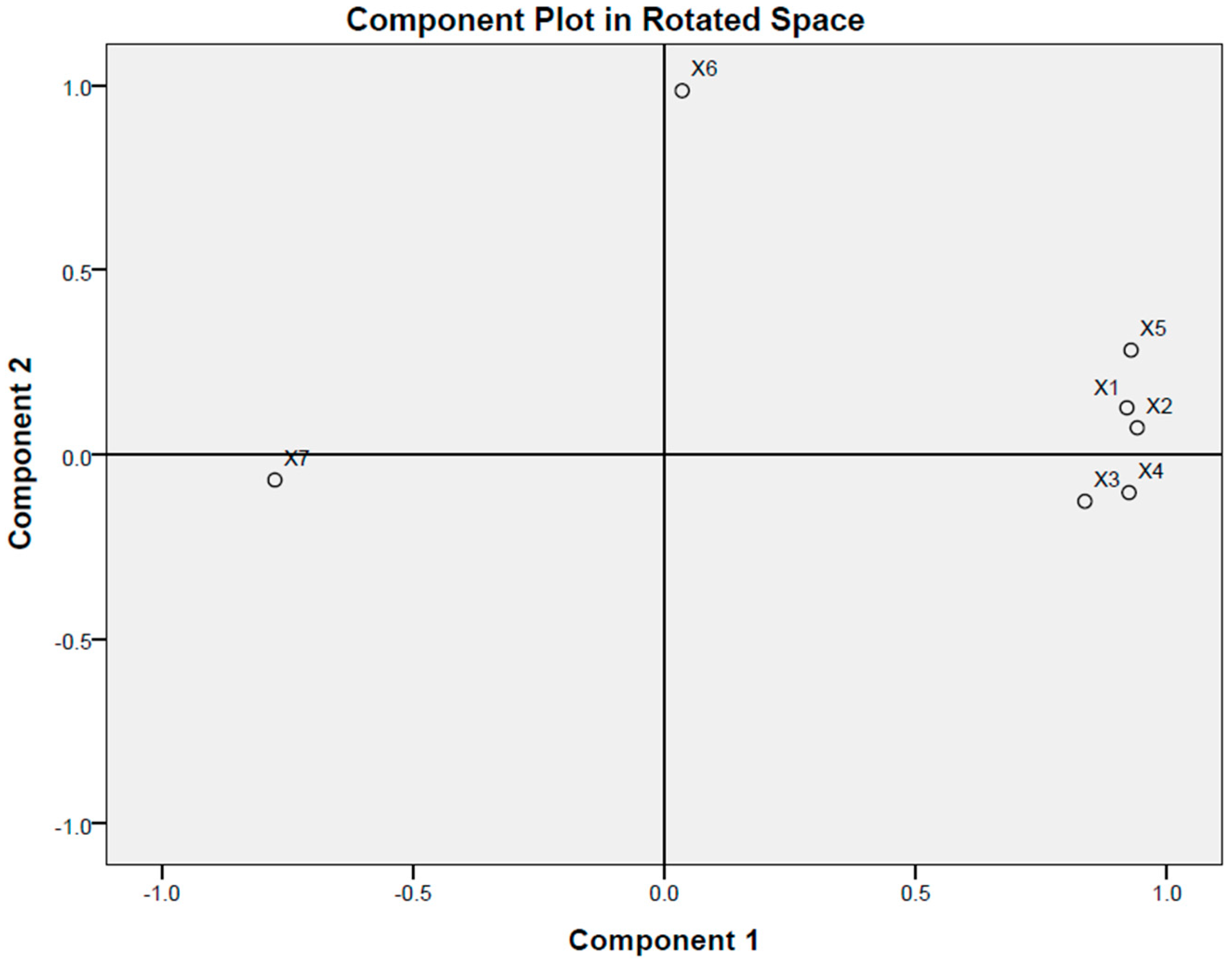
We now examine the direction and magnitude of the coefficients of the original variables in the varimax-rotated component matrix of the PCA dimensional subspace (see Table 3). First, we find that most of the variables in the original dataset load almost uniformly to PC1 in the varimax-rotated component matrix. Given our factor loading threshold of 0.4, it can be said that six of our seven variables load significantly on the first component, and the remaining one loads highly significantly on the second component. This can be interpreted that in general, the seven analyzed bioeconomy subsectors are almost equally important in Japan’s bioeconomy. However, it is important to highlight the variables that exhibit the largest explanatory capacity. According to the varimax-rotated component matrix, PC1 is dominated by variables X2 (0.941) and X5 (0.929) (see Table 3 and Figure 2). Variable X2 and X5 are both forestry and forestry-related products. It is concluded that forestry and forestry-related products such as wood play a leading role in the Japanese bioeconomy. Again, the varimax-rotated component matrix indicates that PC2 has only variable X6 manufacture of paper and paper products (0.975). This underscores another wood-related sector in the Japanese bioeconomy.
Further analysis of the component plot in rotated space (Figure 2) shows two main clusters of variables. First, variables X1 to X5 on PC1 show a high positive coefficient, and they are grouped together. This shows that they are highly correlated, whereas variables X7 (bioenergy) is located at the opposite. Each of these variables shows a high negative coefficient, and this indicates that the two variables are highly correlated. The position of the first and second clusters of variables show that variables X1 to X5 are negatively correlated with variable X7. Variable X6 (manufacture of paper and paper products) exhibits different variance from all the other variables, and it is located on PC2.
4.2. Econometric Model
This study institutes econometric analysis to establish the relationship that exists between the various bioeconomic sectors and the national economy.
4.2.1. Unit Root
As indicated above, the first step of the ARDL bounds test is to establish that none of the variables is integrated with order two. The result for the unit root tests is presented in (Table 4). In the ADF test, we use the Akaike info criterion (AIC) with a maximum of two lags. The critical threshold is 5%.
ADF and PP unit root tests concluded that GDP and PC2 have unit roots when level, but both become stable after the first difference. PC1, on the other hand, is stable when level. This result shows that our variables are integrated with the mix order, but none is integrated with order two. Based on this result, the ARDL bounds test is suitable for the cointegration test.
4.2.2. ARDL Bounds Tests for Cointegration
Base on Equations (3)–(5) presented in Section 3.2.2 above, we estimate the ARDL models one, two, and three, respectively, and the result is presented in Table 5a. We find from the ARDL bounds tests for cointegration analysis that each of the F-test from model one to three is above the 5% critical upper bound. The null hypothesis of no cointegration relationship is rejected, leading to the conclusion that cointegration exists among the variables in each of the models. It can be observed that the F-test in model one to model three are far above their respective upper bounds (see Table 5a), indicating a very strong rejection of the hypothesis. The diagnostic tests for the ARDL models are presented in Table 5b.
The diagnostic tests include the LM test for serial correlation, heteroskedasticity test (ARCH test), Jarque–Bera normality test, and RESET test for stability diagnostics. The p-value of each of the tests is above 5% significant value (see Table 5b). The results of the diagnostic tests show that there are no serial correlation, heteroskedasticity, and normality problems associated with these models. The Ramsey RESET test confirms that the estimated model is stable.
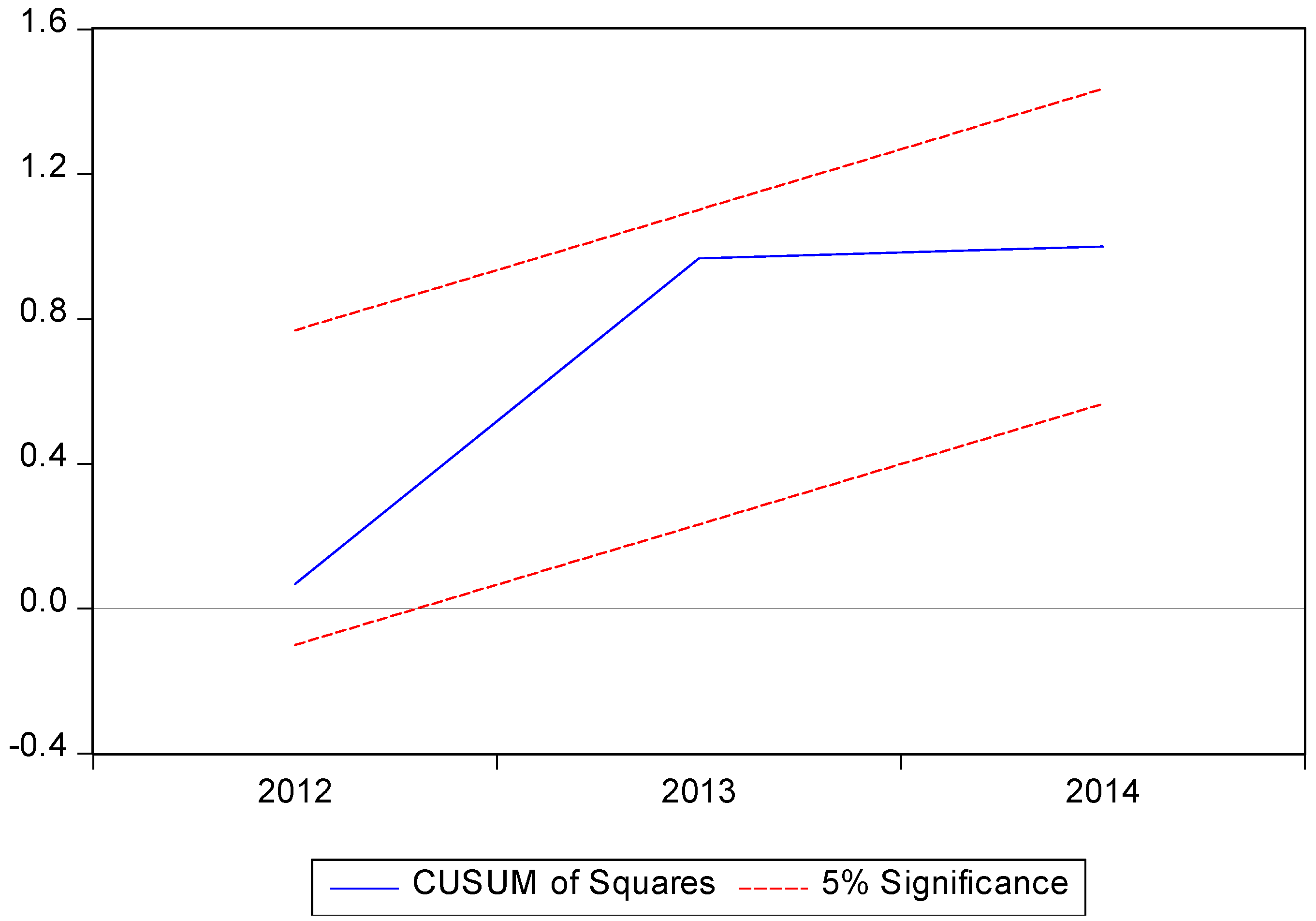
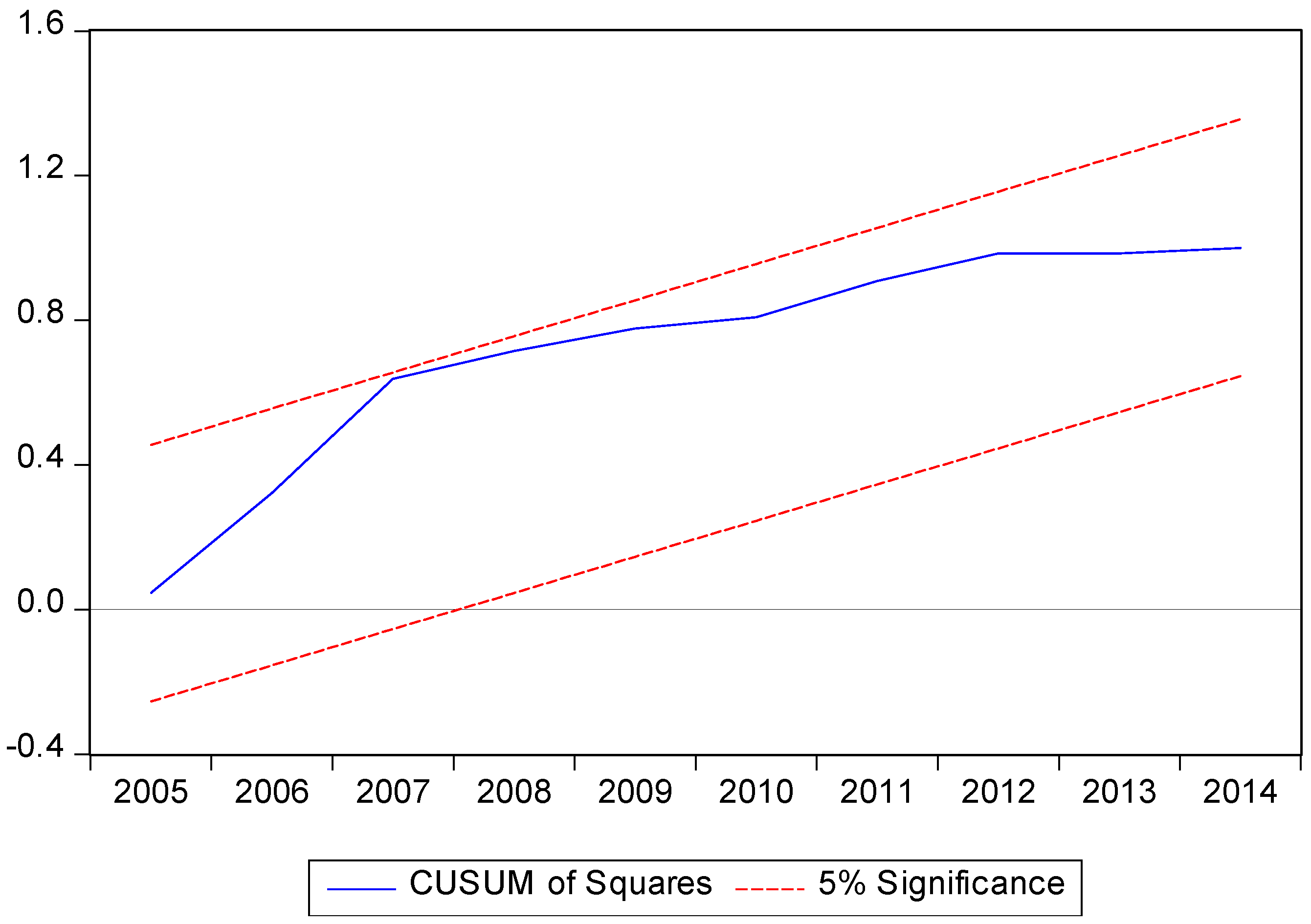
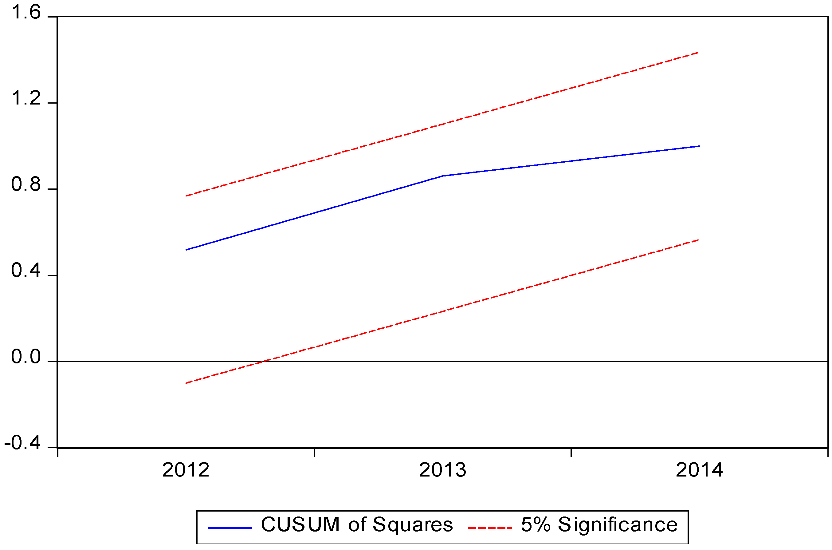
The plots presented in Figure 3, Figure 4 and Figure 5 show that there are no instability issues, since the CUSUMQ statistics fall within the critical bounds at a 5% significance level, indicating that the model has stable parameters over time. The results from the diagnostic tests show that the conclusions reached from the ARDL bounds test can be accepted with confidence, and further analysis can be made.
4.2.3. ARDL Estimated ARDL Short-Run and Long-Run Cointegrating Forms
The estimated ARDL short-run and long-run cointegrating forms for the causality test are presented in Table 6. In the short-run, it can be seen that all the independent variables, including the lagged value of the dependent variable, GDP, are significant except for PC2. It can be seen that the PC2 and PC2 lag (2) value of PC2 has a p-value of 0.071 and 0.095 and are significant, but only at the 10% confident interval. However, per the benchmark of this study, we argue that there is no causal relationship between the two variables, because their respective probability values exceed the 5% critical value benchmark of this study. PC2 lag (1) with a p-value of 0.840 is completely insignificant. The trend and constant terms are also highly significant, justifying their inclusion in the model. Almost all the other variables have positive coefficients, which suggest positive relationships among the variables.
In the long run, PC1 is significant at a 5% critical value, so it retains its economic interpretation, but PC2 is not significant, even at a 10% critical value (see Table 6).
4.2.4. VECM Granger Causality Test
The VECM Granger causality models based on Equations (6)–(8) are presented in Table 7. First, it can be confirmed that there is a short-run unidirectional causality running from PC1 and PC2 to GDP at a 5% critical value, but not vice versa. The short-run causality from PC1 to GDP is a confirmation of the first finding in the ARDL framework. A bidirectional short-run causality is observed between GDP and PC2 at the 10% significant level, but per the benchmark of this paper, we argue that there is no causal relationship between the two variables, because their respective probability values exceed the 5% critical value benchmark of this paper.
It can further be seen that there is no short-run causality from PC2 to PC1, but causality does exist running from PC1 to PC2 at the 5% significance level. Looking at the long-run causality, the ECTt−1 coefficients for each of the three error correction models is negative and statistically significant. With GDP as the dependent variable, long-run causality runs from the explanatory variables, PC1 and PC2, at a 1% significance level (see Table 7). Similarly, with either PC1 or PC2 as the dependable variable, a long-run causality exists among all the variables at a 5% significance level.
5. Discussion
The findings from this study show that most of the bioeconomy subsectors contribute significantly and almost uniformly to the GDP growth in Japan. This finding implies that Japan needs to handle her bioeconomy in a holistic approach rather than a sector-specific approach. According to the World BioEconomy Forum [52], various countries have prioritized specific sectors of their bioeconomy to achieve specific targets. However, the findings in this study suggest that Japan must not leave any of the bioeconomy sectors behind in her quest to develop and achieve their bioeconomy targets.
This present study further establishes that among the significant contributing sectors of the bioeconomy, forestry and logging and wood products are the leading sectors of the bioeconomy in Japan. This finding is largely consistent with previous studies such as [53], and this suggests that bioeconomy output in Japan is still dominated by primary production. This finding also confirms the assertion made by [54] that traditional bioeconomy sectors dominate the bioeconomy. This may not be surprising, because the bioeconomy concept itself is based on biological materials that are usually generated from forestry and agriculture products. The finding that forestry and forest products are the leading bioeconomy sectors in Japan is very reflective of the happenings in the Asian country. Japan has strategies and plans that are directed exclusively at the production and industrial use of biomass [55]. Recently developed policies include The National Plan for the Promotion of Biomass Utilization [56]. Precisely, in relation to biomass for energy, the focus of this national strategy is on woody biomass in distributed energy systems and next-generation biofuels. This has caused a surge in imported and domestically produced wood pellets to meet the needs of power plants in the future [57]. Also, there is significant potential for biomass usage in Japan in the future, especially with the considerable amount of wasted wood [57]. Due to the high focus on bioenergy in Japan, we anticipated finding a higher coefficient for bioenergy in relation to the other sectors, but surprisingly, we found that bioenergy had the least coefficient among the sectors in this study. This may be due to the smaller size of bioenergy in comparison with other huge sectors such as forestry, agriculture, etc.
This study confirms that, in Japan, long-run cointegration and causal relationships exist between the bioeconomy subsectors and the GDP growth in each of the three models. However, the short-run relationship cannot be confirmed in two out of the three models. One possible reason for this finding is that the concept of bioeconomy is long-term in nature [58], and has not yet unleashed its full potential [25]. Another important reason may be that bioproducts have not fully hit commercialization [59], and consumers are generally unfamiliar with bio-based products [60]. Bioproducts are currently being promoted by policymakers as policymakers map up strategies [4] to realize bioeconomy dreams, but this initiative would be more successful if it was led by the market.
Given the inherent sustainability assumption in bioeconomy [2], this study shows that bioeconomy has the capacity to significantly impact the sustainable development of Japan. To achieve this, policymakers need to pursue bioeconomy with profitability concerns as a major target to be able to attract industry, without which bioeconomy will remain an abstract notion [61], and the desired sustainable development may elude us.
This study aims by no means to be exhaustive, nor claims to be representative of the entire bioeconomy discussion in Japan. Given the broad nature of bioeconomy, this study has focused on only seven selected sectors of bioeconomy.
6. Conclusions
Our study utilized recent econometric techniques such as the autoregressive distributed lag (ARDL) and VECM Granger causality model to reveal the direction of the causality among the variables within the current study period. Our study also utilized probably the most popular multivariate statistical technique, principal component analysis (PCA), to elucidate the relationship among our independent variables.
Principal component analysis was first used to identify the bioeconomy sectors that contribute significantly to the GDP growth of Japan. The PCA yielded two principal components that explain 83.6% of the variations in the seven bioeconomy sectors. We found from the PCA that all of the bioeconomy sectors contribute almost uniformly to the GDP growth of Japan. In view of this finding, this study calls for a holistic development of the Japanese bioeconomy where all of the sectors are properly linked, since they are all almost equally important and interdependent. By ranking the Japanese bioeconomy sectors through the Varimax rotation method, this study finds that the paramount influencing bioeconomy sectors are forestry, logging, wood, and food products. Surprisingly, we find bioenergy to be the lowest contributor, even though it has received the most policy attention in Japan.
In a further analysis, we instituted the ARDL bounds test of cointegration with the two selected principal components as independent variables and GDP as a dependent variable. The test proved the existence of long-run relationships among all the variables, which means the Japanese bioeconomy and their GDP growth move together in the long run. In further analysis, the VECM Granger causality test showed that there exists a short-run causality running from PC1 and PC2 to GDP, but not vice versa. However, long-run causality was established among the three variables. The leading sectors in PC1 are forestry, logging, wood, and food products, and that of PC2 is the manufacture of paper and paper products. This confirms that the Japanese bioeconomy is still heavily dominated by primary production. We recommend a policy direction that seeks to promote high-value bioproducts in order to achieve the sustainable economic growth that is needed in Japan.
Author Contributions
D.Q. (Daniel Quacoe) conceived and designed the paper; X.W. supervised the paper, D.Q. (Daniel Quacoe) and D.Q. (Dinah Quacoe) collected, processed and analyzed the data; D.Q. (Daniel Quacoe), K.A. and B.A.D. interpreted the results; D.Q. (Daniel Quacoe) wrote the paper.
Funding
The study was funded by Major Research Project of Philosophy and Social Science in Colleges and Universities of Jiangsu Province (No. 2018SJZDA006) and Research Project of The Social Science Foundation of Jiangsu Province (No. 18GLB012).
Acknowledgments
We are sincerely grateful to Henry Asante Antwi and Kofi Baah Boamah of Jiangsu University as well as Samuel Owusu Mensah of Jinggangshan University for their insightful contributions.
Conflicts of Interest
The authors declare no conflict of interest
Appendix A
| X1 | Agriculture |
| X2 | Forestry and logging |
| X3 | Fishing and aquaculture |
| X4 | Manufacture of food products, beverages and tobacco products |
| X5 | Manufacture of wood and of products of wood and cork, except furniture; manufacture of articles of straw and plaiting materials |
| X6 | Manufacture of paper and paper products |
| X7 | Bioenergy |
References
- Demirbas, M.F. Current technologies for biomass conversion into chemicals and fuels, Part A: Recovery, Utilization, and Environmental Effects. Energy Sources 2006, 28, 1181–1188. [Google Scholar] [CrossRef]
- Pfau, S.F.; Hagens, J.E.; Dankbaar, B.; Smits, A.J.M. Visions of sustainability in bioeconomy research. Sustainability 2014, 6, 1222–1249. [Google Scholar] [CrossRef]
- NASA. Global Climate Change 2018. Available online: https://climate.nasa.gov/causes/ (accessed on 18 November 2018).
- European Commission. The Bioeconomy Strategy. 2012. Available online: https://ec.europa.eu/research/bioeconomy/index.cfm?pg=policy&lib=strategy (accessed on 7 August 2018).
- Staffas, L.; Gustavsson, M.; McCormick, K. Strategies and policies for the bioeconomy and bio-based economy: An analysis of official national approaches. Sustainability 2013, 5, 2751–2769. [Google Scholar] [CrossRef]
- European Commission-Press Release Data Base (February 2012). Commission Adopts Its Strategy for a Sustainable Bioeconomy to Ensure Smart Green Growth in Europe. MEMO/12/97. 2012. Available online: http://europa.eu/rapid/press-release_MEMO-12-97_en.htm?locale¼en (accessed on 9 November 2018).
- GBS. Global Bioeconomy Summit Communiqué. 2018. Available online: http://gbs2018.com/home/ (accessed on 1 November 2018).
- Van Lancker, J.; Wauters, E.; Van Huylenbroeck, G. Managing innovation in the bioeconomy: An open innovation perspective. Biomass Bioenergy 2016, 90, 60–69. [Google Scholar] [CrossRef]
- Dubois, O.; Gomez San Juan, M. How Sustainability is Addressed in Official Bioeconomy Strategies at International, National and Regional Levels: An Overview; Environment and Natural Resources Management Working Paper no. 63; FAO: Roma, Italy, 2016. [Google Scholar]
- Birch, K.; Tyfield, D. Theorizing the Bioeconomy: Biovalue, Biocapital, Bioeconomics or… What? Sci. Technol. Hum. Values 2013, 38, 299–327. [Google Scholar] [CrossRef]
- Birch, K. The problem of bio-concepts: Biopolitics, bio-economy and the political economy of nothing. Cult. Stud. Sci. Educ. 2017, 12, 915–927. [Google Scholar] [CrossRef]
- Sheppard, A.W.; Gillespie, I.; Hirsch, M.; Begley, C. Biosecurity and sustainability within the growing global bioeconomy. Curr. Opin. Environ. Sustain. 2011, 3, 4–10. [Google Scholar] [CrossRef]
- Gottwald, F.; Budde, J. Mit Bioökonomie die Welt ernähren; Institut für Welternährung–World Food Institute eV: Berlin, Germany, 2015. [Google Scholar]
- Conference Series LLC Ltd. 14th International Conference on Biofuels, Energy & Economy. 2018. Available online: https://biofuels-bioenergy.conferenceseries.com/ (accessed on 18 November 2018).
- U.S. Energy Information Administration. Biomass Explained. 2018. Available online: https://www.eia.gov/energyexplained/?page=biomass_home (accessed on 18 November 2018).
- Moore, A. Biofuels are dead: Long live biofuels (?)–Part one. New Biotechnol. 2008, 25, 6–12. [Google Scholar] [CrossRef] [PubMed]
- Simpson-Holley, M.; Higson, A.; Evans, G. Bring on the biorefinery. Chem. Eng. 2007, 795, 46–48. [Google Scholar]
- Demirbas, A. Fuels from Biomass. Available online: https://0-link-springer-com.brum.beds.ac.uk/chapter/10.1007/978-1-84882-721-9_2 (accessed on 29 January 2019).
- Staub, A.; Guillarme, D.; Schappler, J.; Veuthey, J.-L.; Rudaz, S. Intact protein analysis in the biopharmaceutical field. J. Pharm. Biomed. Anal. 2011, 55, 810–822. [Google Scholar] [CrossRef]
- Shakeri, R.; Radfar, R. Antecedents of strategic alliances performance in biopharmaceutical industry: A comprehensive model. Technol. Forecast. Soc. Chang. 2017, 122, 289–302. [Google Scholar] [CrossRef]
- Watier, H. Biotherapies, immunotherapies, targeted therapies, biopharmaceuticals… which word should be used? Med. Sci. 2014, 30, 567–575. [Google Scholar]
- McKinsey. Rapid Growth in Biopharma: Challenges and Opportunities Current Developments in Biotechnology and Bioengineering: Human and Animal Health Applications 2014. Available online: https://www.mckinsey.com/industries/pharmaceuticals-and-medical-products/our-insights/rapid-growth-in-biopharma (accessed on 19 November 2018).
- Rohrbeck, M.; Körsten, S.; Fischer, C.B.; Wehner, S.; Kessler, B. Diamond-like carbon coating of a pure bioplastic foil. Thin Solid Films 2013, 545, 558–563. [Google Scholar] [CrossRef]
- European BioPlastics. Bioplastics Production Capacities to Grow by more than 400% by 2018. 2014. Available online: http://news.bio-based.eu/bioplastics-production-capacities-grow-400-2018/ (accessed on 19 November 2018).
- Fuentes-Saguar, P.D.; Mainar-Causapé, A.J.; Ferrari, E. The role of bioeconomy sectors and natural resources in EU economies: A social accounting matrix-based analysis approach. Sustainability 2017, 9, 2383. [Google Scholar] [CrossRef]
- German Bioeconomy Council. Future Opportunities and Developments in the Bioeconomy—A Global Expert Survey. Available online: https://gbs2018.com/fileadmin/gbs2018/Downloads/Bioeconomy_Global_Expert_Survey.pdf (accessed on 4 August 2018).
- Kharas, H. The Emerging Middle Class in Developing Countries; OECD Development Centre: Paris, France, 2010. [Google Scholar]
- D’Hondt, K.; Jiménez-Sánchez, G.; Philp, J. Reconciling Food and Industrial Needs for an Asian Bioeconomy: The Enabling Power of Genomics and Biotechnology. Asian Biotechnol. Dev. Rev. 2015, 17, 85–130. [Google Scholar]
- El-Chichakli, B.; Von Braun, J.; Lang, C.; Barben, D.; Philp, J. Policy: Five cornerstones of a global bioeconomy. Nat. News 2016, 535, 221. [Google Scholar] [CrossRef]
- Lee, D.-H. Bio-based economies in Asia: Economic analysis of development of bio-based industry in China, India, Japan, Korea, Malaysia and Taiwan. Int. J. Hydrogen Energy 2016, 41, 4333–4346. [Google Scholar] [CrossRef]
- World Bank Group. Gross Domestic Product 2017. Available online: http://databank.worldbank.org/data/download/GDP.pdf (accessed on 4 December 2018).
- Plessis, L.D. Japan’s Biomass Market Overview. Japan External Trade Organization (JETRO). 2015. Available online: https://www.jetro.go.jp/ext_images/_Events/ldn/Japan_biomass_market_overview.pdf (accessed on 4 December 2018).
- ISEP. The Share of Renewable Energy in Total Power Generation in Japan in 2015. Available online: https://www.isep.or.jp/en/library/3362 (accessed on 12 January 2019).
- World Bank. Forest Area (% of Land Area). 2015. Available online: http://data.worldbank.org/indicator/AG.LND.FRST.ZS (accessed on 4 December 2018).
- Yanagida, T. System evaluation for sustainable bioenergy production. In Proceedings of the 3rd ACMECS Bioenergy Workshop, Future Development of ACMECs Bioenergy/Regional Plan and Standardization, Ubon Ratchathani, Thailand, 8–11 December 2015. [Google Scholar]
- Yanagida, T.; Yoshida, T.; Kuboyama, H.; Jinkawa, M. Relationship between feedstock price and break-even point of woody biomass power generation under FIT program. J. Jpn. Inst. Energy 2015, 94, 311–320. [Google Scholar] [CrossRef]
- Timmer, M.P.; Los, B.; Stehrer, R.; De Vries, G.J. An Anatomy of the Global Trade Slowdown Based on the WIOD 2016 Release; Groningen Growth and Development Centre, University of Groningen: Groningen, The Netherlands, 2016. [Google Scholar]
- Asada, R.; Stern, T. Competitive Bioeconomy? Comparing Bio-based and Non-bio-based Primary Sectors of the World. Ecol. Econ. 2018, 149, 120–128. [Google Scholar]
- U.S. Bureau of Economic Analysis. FAQ: “What is Gross Output by Industry?”. Available online: https://www.bea.gov/faq/index.cfm?faq_id=1034 (accessed on 6 June 2018).
- The International Renewable Energy Agency (IRENA). Statistics Time Series. 2018. Available online: http://resourceirena.irena.org/gateway/dashboard/ (accessed on 15 October 2018).
- The World Bank Group. GDP (Current US$). 2018. Available online: https://data.worldbank.org/indicator/ny.gdp.mktp.cd (accessed on 22 November 2018).
- Smeets, E.M.W.; Tsiropoulos, Y.; Patel, M.; Hetemäki, L.; Bringezu, S.; Banse, M.A.H.; Junker, F.; Nowicki, P.; Leeuwen, M.G.A.; van Verburg, P. The Relationship between Bioeconomy Sectors and the Rest of the Economy; SAT-BBE/LEI Wageningen UR; Wageningen University & Research: Wageningen, The Netherlands, 2013. [Google Scholar]
- Jolliffe, I.T.; Stephenson, D.B. Forecast Verification: A Practitioner’s Guide in Atmospheric Science; John Wiley & Sons.: Hoboken, NJ, USA, 2003. [Google Scholar]
- Polyak, B.T.; Khlebnikov, M.V. Robust Principal Component Analysis: An IRLS Approach. IFAC-PapersOnLine 2017, 50, 2762–2767. [Google Scholar] [CrossRef]
- Golub, G.H.; Reinsch, C. Singular value decomposition and least squares solutions. Numer. Math. 1970, 14, 403–420. [Google Scholar] [CrossRef]
- Hutcheson, G.D.; Sofroniou, N. The Multivariate Social Scientist: Introductory Statistics Using Generalized Linear Models; SAGE: Thousand Oaks, CA, USA, 1999. [Google Scholar]
- Barrett, K.; Morgan, G. SPSS for Intermediate Statistics; Use and Interpretation; Lawrence Erlbaum Assocıates: Mahwah, NJ, USA; London, UK, 2005. [Google Scholar]
- Kaiser, H.F. The application of electronic computers to factor analysis. Educ. Psychol. Meas. 1960, 20, 141–151. [Google Scholar] [CrossRef]
- Cattell, R.B.; Jaspers, J. A general plasmode (No. 30-10-5-2) for factor analytic exercises and research. Multivar. Behav. Res. Monogr. 1967, 67, 211. [Google Scholar]
- Pesaran, M.H.; Shin, Y.; Smith, R.J. Bounds testing approaches to the analysis of level relationships. J. Appl. Econ. 2001, 16, 289–326. [Google Scholar] [CrossRef] [Green Version]
- Granger, C.W. Some recent development in a concept of causality. J. Econ. 1988, 39, 199–211. [Google Scholar] [CrossRef]
- World BioEconomy Forum. The Bioeconomy Celebrates Nature. Available online: http://www.wcbef.com/ (accessed on 7 August 2018).
- Efken, J.; Dirksmeyer, W.; Kreins, P.; Knecht, M. Measuring the importance of the bioeconomy in Germany: Concept and illustration. NJAS-Wageningen J. Life Sci. 2016, 77, 9–17. [Google Scholar] [CrossRef]
- Meyer, R. Bioeconomy strategies: Contexts, visions, guiding implementation principles and resulting debates. Sustainability 2017, 9, 1031. [Google Scholar] [CrossRef]
- German Bioeconomy Council. Bioeconomy-Policy Part-I, Synopsis and Analysis of Strategies in the G7. 2015. Available online: http://biooekonomierat.de/fileadmin/international/Bioeconomy-Policy_Part-I.pdf (accessed on 2 August 2018).
- Ministry of Agriculture, Forestry, and Fisheries. The Guidebook for Promoting Biomass Town Concept. 2013. Available online: http://www.maff.go.jp/e/pdf/contents.pdf (accessed on 8 August 2018).
- Pambudi, N.A.; Itaoka, K.; Chapman, A.; Hoa, N.D.; Yamakawa, N. Biomass energy in Japan: Current status and future potential. Int. J. Smart Grid Clean Energy 2017, 6, 119–126. [Google Scholar] [CrossRef]
- German Presidency. En Route to the Knowledge-Based Bio-Economy. 2007. Available online: https://dechema.de/dechema_media/Cologne_Paper-p-20000945.pdf (accessed on 16 November 2018).
- Chandel, A.K.; Garlapati, V.K.; Singh, A.K.; Antunes, F.A.F.; Da Silva, S.S. The path forward for lignocellulose biorefineries: Bottlenecks, solutions, and perspective on commercialization. Bioresour. Technol. 2018, 264, 370–381. [Google Scholar] [CrossRef]
- Sijtsema, S.J.; Onwezen, M.C.; Reinders, M.J.; Dagevos, H.; Partanen, A.; Meeusen, M. Consumer perception of bio-based products—An exploratory study in 5 European countries. NJAS-Wageningen J. Life Sci. 2016, 77, 61–69. [Google Scholar] [CrossRef]
- Sillanpää, M.; Ncibi, C. Bioeconomy: The Path to Sustainability. In A Sustainable Bioeconomy; Springer: Cham, Switzerland, 2017; pp. 29–53. [Google Scholar]
Figure 1.
Scree plot. Source: Authors’ computation.

Figure 2.
Component plot in varimax-rotated space. Source: Authors’ computation.

Figure 3.
Cumulative sum of squares (CUSUM) plots and tests for model one. Source: Authors’ computation.
Figure 3.
Cumulative sum of squares (CUSUM) plots and tests for model one. Source: Authors’ computation.

Figure 4.
CUSUM plots and tests for model two. Source: Authors’ computation.

Figure 5.
CUSUM plots and tests for model three. Source: Authors’ computation.


Table 1.
Kaiser–Meyer–Olkin (KMO) and Bartlett’s test.
| Kaiser–Meyer–Olkin Measure of Sampling Adequacy: | 0.67 | ||||
| Bartlett’s test of sphericity; | Approx. Chi-Square: | 97.20 | |||
| Df: | 21 | ||||
| Sig: | 0.000 | ||||
Source: Authors’ computation.
Table 2.
Summary of principal component analysis.
| Component | Total | % of Variance | Cumulative % | Total | % of Variance | Cumulative % |
|---|---|---|---|---|---|---|
| 1 | 4.782 | 68.317 | 68.317 | 4.752 | 67.887 | 67.887 |
| 2 | 1.073 | 15.332 | 83.649 | 1.103 | 15.762 | 83.649 |
| 3 | 0.631 | 9.014 | 92.663 | |||
| 4 | 0.275 | 3.933 | 96.596 | |||
| 5 | 0.17 | 2.421 | 99.018 | |||
| 6 | 0.053 | 0.755 | 99.773 | |||
| 7 | 0.016 | 0.227 | 100 | |||
Extraction method: Principal component analysis. Source: Authors’ computation using SPSS.
Table 3.
Varimax rotated component matrix.
| Component | ||
|---|---|---|
| Variable | 1 | 2 |
| X2 | 0.941 | - |
| X5 | 0.929 | - |
| X4 | 0.925 | - |
| X1 | 0.920 | - |
| X3 | 0.837 | - |
| X7 | –0.775 | - |
| X6 | - | 0.975 |
Extraction Method: Principal component analysis. Rotation method: Varimax. Source: Authors’ computation.
Table 4.
Unit root. ADF: augmented Dickey–Fuller, PP: Phillips–Perron.
| ADF | PP | |||||
|---|---|---|---|---|---|---|
| Variable | Level | 1st diff. | CV at 5% | Level | 1st diff. | CV at 5% |
| GDP | –2.254 | −3.199 | −3.119 | −2.266 | −3.503 | −3.119 |
| PC1 | −2.987 | −3.559 | −3.119 | −3.437 | −3.428 | −3.119 |
| PC2 | −1.853 | −3.282 | −3.119 | −1.932 | −3.614 | −3.119 |
Notes: (1) Both ADF and PP tests include an intercept but no trend. (2) Automatic lag selection for. ADF was done by the Akaike info criterion (AIC). Source: Authors’ computation.
Table 5.
Autoregressive distributed lag (ARDL) bounds tests for cointegration; (a) 5% Critical Bounds; (b) Diagnostic tests.
Table 5.
Autoregressive distributed lag (ARDL) bounds tests for cointegration; (a) 5% Critical Bounds; (b) Diagnostic tests.
| (a) | ||||
| Model | F-test | Lower | Upper | Conclusion |
| Model 1 | 12.188 | 3.88 | 4.61 | Cointegration *** |
| Model 2 | 9.243 | 3.10 | 3.87 | Cointegration *** |
| Model 3 | 23.676 | 4.87 | 5.85 | Cointegration *** |
| (b) | ||||
| Equation | LM Test | Hetero. | Jarque–Bera | RESET Test |
| Model 1 | 3.944 (0.33) | 3.753 (0.15) | 0.362 (0.83) | 2.537 (0.26) |
| Model 2 | 2.351 (0.16) | 1.091 (0.39) | 0.832 (0.65) | 0.728 (0.49) |
| Model 3 | 5.099 (0.29) | 5.805 (0.09) | 0.682 (0.71) | 0.474 (0.56) |
Note: *** and ** in Table 5(a) denote rejection of the hypothesis at 1% and 5% critical bounds, respectively. The AIC is used to determine the optimal lag. The ARDL model in Table 5(a) is estimated by using unrestricted constant and unrestricted trend (case five). The tests in Table 5(b) present t-statistics and their respective p-value in parenthesis at the 5% critical value. Source: Authors’ computation.
Table 6.
Estimated ARDL short-run and long-run cointegrating forms.
| Short-Run Cointegrating Form | ||||
| Variable | Coefficient | Std. Error | t-Statistic | Prob. |
| D(GDP(–1)) | 1.200 | 0.230 | 5.216 ** | 0.013 |
| D(GDP(–2)) | –1.723 | 0.270 | –6.488 ** | 0.007 |
| D(PC1) | 0.362 | 0.480 | 0.753 ** | 0.006 |
| D(PC1(–1)) | 0.834 | 0.634 | 1.315 ** | 0.040 |
| D(PC1(–2)) | 0.343 | 0.730 | 3.207 ** | 0.049 |
| D(PC2) | 0.759 | 0.277 | 2.739 | 0.071 |
| D(PC2(–1)) | 0.035 | 0.167 | 0.207 | 0.840 |
| D(PC2(–2)) | –0.285 | 0.118 | –2.409 | 0.095 |
| C | –8.928 | 2.145 | –4.161 | 0.023 |
| D(@TREND) | 1.096 | 0.275 | 4.257 | 0.023 |
| Long-Run Cointegrating Form | ||||
| Variable | Coefficient | Std. Error | t-Statistic | Prob. |
| PC1 | 0.322 | 0.701 | 3.3 | 0.045 ** |
| PC2 | 0.334 | 0.207 | 1.612 | 0.205 |
Note: ** represent significance level at 5% level. Source: Authors’ computation.
Table 7.
VECM Granger causality test.
| Dependent | ΔGDP | ΔPC1 | ΔPC2 | ECTt−1 |
|---|---|---|---|---|
| ΔGDP | - | 0.362 (0.042) ** | 0.759 (0.018) ** | –1.524 (–8.383) ** |
| ΔPC1 | 0.362 (0.442) | - | 2.342 (0.172) | –0.262 (–6.933) *** |
| ΔPC2 | 6.088 (0.09) * | 2.129 (0.014) ** | - | –0.761 (–10.308) ** |
Notes: ***, **, * Significant at 1%, 5%, and 10% levels, respectively. Source: Authors’ computation.
© 2019 by the authors. Licensee MDPI, Basel, Switzerland. This article is an open access article distributed under the terms and conditions of the Creative Commons Attribution (CC BY) license (http://creativecommons.org/licenses/by/4.0/).
Share and Cite
MDPI and ACS Style
Wen, X.; Quacoe, D.; Quacoe, D.; Appiah, K.; Ada Danso, B. Analysis on Bioeconomy’s Contribution to GDP: Evidence from Japan. Sustainability 2019, 11, 712. https://0-doi-org.brum.beds.ac.uk/10.3390/su11030712
AMA Style
Wen X, Quacoe D, Quacoe D, Appiah K, Ada Danso B. Analysis on Bioeconomy’s Contribution to GDP: Evidence from Japan. Sustainability. 2019; 11(3):712. https://0-doi-org.brum.beds.ac.uk/10.3390/su11030712
Chicago/Turabian StyleWen, Xuezhou, Daniel Quacoe, Dinah Quacoe, Kingsley Appiah, and Bertha Ada Danso. 2019. "Analysis on Bioeconomy’s Contribution to GDP: Evidence from Japan" Sustainability 11, no. 3: 712. https://0-doi-org.brum.beds.ac.uk/10.3390/su11030712
Note that from the first issue of 2016, this journal uses article numbers instead of page numbers. See further details here.