Article

A Novel Hyper-Heuristic for the Biobjective Regional Low-Carbon Location-Routing Problem with Multiple Constraints

1
Key Laboratory of Special Equipment Manufacturing and Advanced Processing Technology, Ministry of Education, Zhejiang University of Technology, Hangzhou 310023, China
2
College of Computer Science and Technology, Zhejiang University of Technology, Hangzhou 310023, China
*
Author to whom correspondence should be addressed.
Sustainability 2019, 11(6), 1596; https://0-doi-org.brum.beds.ac.uk/10.3390/su11061596
Submission received: 25 January 2019 / Revised: 12 March 2019 / Accepted: 13 March 2019 / Published: 15 March 2019
(This article belongs to the Section Sustainable Transportation)

Abstract

:
With the aim of reducing cost, carbon emissions, and service periods and improving clients’ satisfaction with the logistics network, this paper investigates the optimization of a variant of the location-routing problem (LRP), namely the regional low-carbon LRP (RLCLRP), considering simultaneous pickup and delivery, hard time windows, and a heterogeneous fleet. In order to solve this problem, we construct a biobjective model for the RLCLRP with minimum total cost consisting of depot, vehicle rental, fuel consumption, carbon emission costs, and vehicle waiting time. This paper further proposes a novel hyper-heuristic (HH) method to tackle the biobjective model. The presented method applies a quantum-based approach as a high-level selection strategy and the great deluge, late acceptance, and environmental selection as the acceptance criteria. We examine the superior efficiency of the proposed approach and model by conducting numerical experiments using different instances. Additionally, several managerial insights are provided for logistics enterprises to plan and design a distribution network by extensively analyzing the effects of various domain parameters such as depot cost and location, client distribution, and fleet composition on key performance indicators including fuel consumption, carbon emissions, logistics costs, and travel distance and time.

1. Introduction

City logistics, particularly in the context of freight transportation, exert pressure on the economy, society, environment, and citizens [1]. Among several tools of logistic network design, the traveling salesman problem (TSP) [2], the vehicle-routing problem (VRP) [3], and the location-routing problem (LRP) [4] are the most important and widely studied combinatorial optimization problems, especially the LRP. However, these basic tools are incapable of addressing sustainable development for the economy, society, and the environment simultaneously. Recently, premutation and coordination of the joint bond of economic, social, and environmental benefits have emerged as one of the most addressed problems. This inspires us to model the LRP by considering the environmental effect, which aims to reduce cost, shorten the service period, and reduce greenhouse gases (GHG) emissions, especially CO2.
Zhang et al. [5] first introduced the term low-carbon LRP (LCLRP) in 2017, in which the goal is to reduce carbon emission (CE) composed of depots’ fixed CE and vehicles’ traveling CE, by optimizing the sets of depots to open and tracings of the routes. Koc et al. [1] developed a regional LCLRP (RLCLRP) as a single objective to assess the effects of depots, clients, and fleets on logistics cost, fuel consumption and CE (FCCE). The authors applied a penalty function to the transfer fuel consumption cost. Our previous study [6] used the same method and considered a series of real-world requirements for the RLCLRP, such as hard time windows (HTW), simultaneous pickup and delivery (SPD), and a heterogeneous fleet (HF). This paper is based on the works of Koc et al. [1] and Leng et al. [6]. Without a doubt, there are important differences among these three works. This paper defines a biobjective model for the RLCLRP whereas the others addressed a single objective. The solution approach in this paper is a quantum-inspired multiobjective hyper-heuristic (MOHH), while the approaches in our previous work and Koc et al. [1] were, respectively, single-objective hyper-heuristics and adaptive large neighborhood search metaheuristic. Besides, the real-world conditions in this paper are different those in the work of Koc et al. [1]. The main contributions of this paper are as follows:
  • Problem domain. We first consider biobjective optimization for the RLCLRP with simultaneous pickup and delivery, hard time windows, and a heterogeneous fleet.
  • Problem model. A novel and simple mixed-integer programming model is defined.
  • Solution method. This work develops a quantum-inspired selection strategy (QS) as a high-level heuristic in the framework of MOHH.
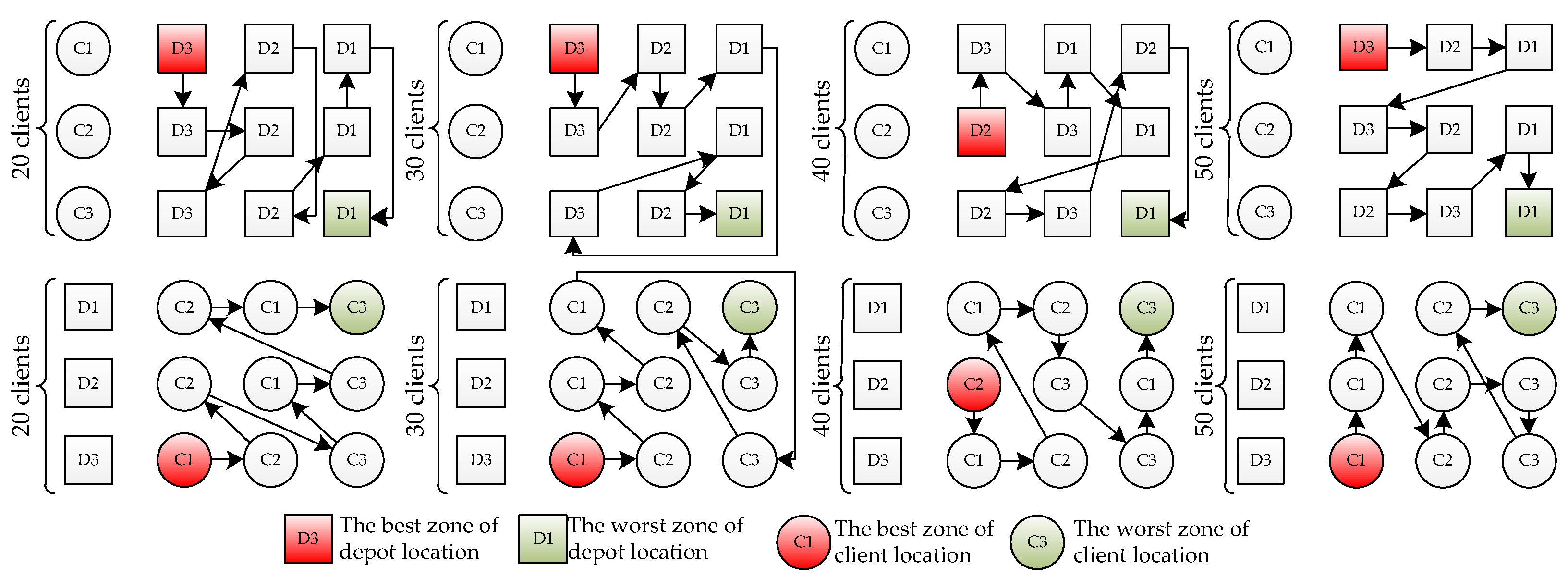
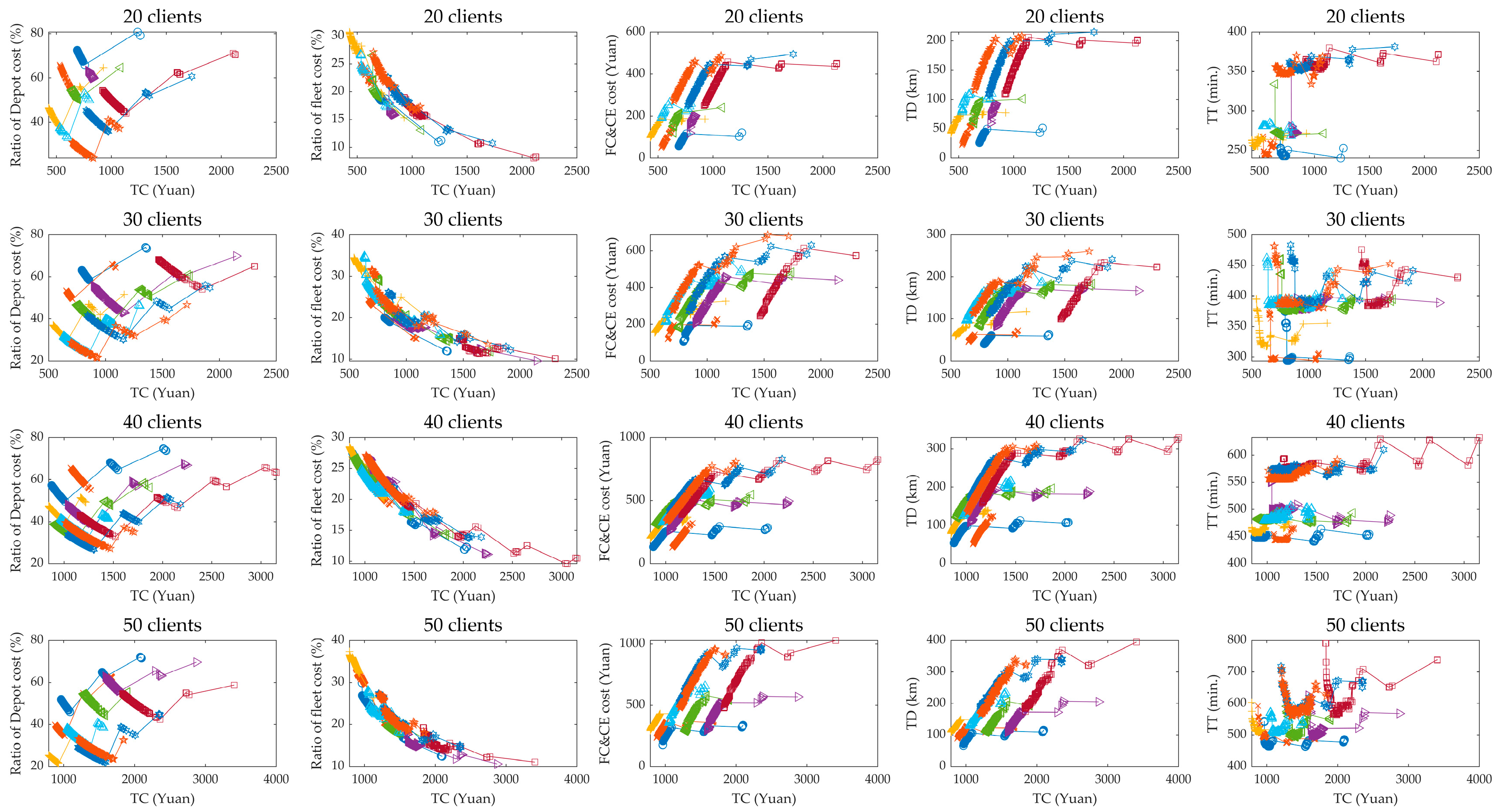
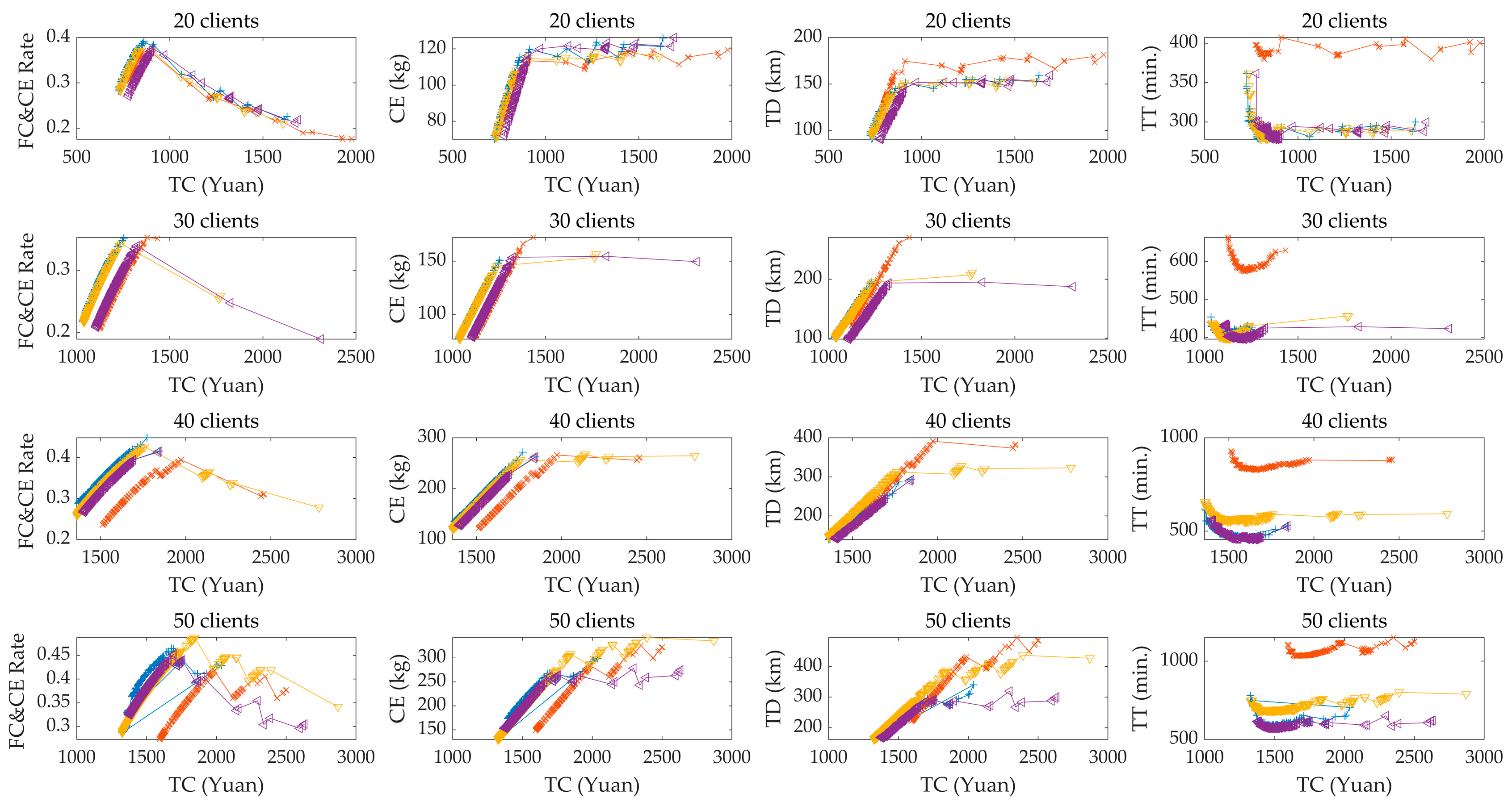
  • Managerial insights. This paper provides several management suggestions by analyzing the effects of depots, clients, and fleet composition on key performance indicators, such as travel distance, travel time, CE, and operational cost.
The remainder of this work is organized as follows. Section 2 reviews the literature of the domain problem and the proposed heuristics. Section 3 defines the problem description and biobjective model. Section 4 details the proposed methods. Experiments and evaluation are given in Section 5, and, finally, conclusions are presented in Section 6.

2. Literature Review

2.1. Fuel Consumption and Carbon Emission Review

The LRP simultaneously handles two types of NP-hard decisions that are often addressed in logistics: the location-allocation problem (LAP) and the VRP [6,7]. Among the various versions of the LRP in the literature, the LRP considering environmental effect (LCLRP) has gained many researchers’ attention because environmental effects have a strong relationship to economic and social sustainability and even to public health. Similarly, the LCLRP is a more complicated NP-hard problem comprising of the LAP and the VRP with environmental effects, referred to as the pollution-routing problem (PRP) [8], green vehicle-routing problem (GVRP) [9], or eco-routing problem (ERP) [10].
In applications of the LCLRP, the most significant estimation is that of the amount of FCCE [11]. As Demir et al. [12] stated, estimation and reduction of FCCE require accurate, real-time models to heighten the logistics efficiency. Also, the nature and types of various FCCE estimation models determine the application range, because transportation activity and traffic conditions are uncertain factors. As the public requires higher air quality, three types of models [13] have been developed:
  • In factors models, only few key factors are considered, such as travel distance and vehicle load. Examples are the fuel consumption rate (FCR) [5,14,15,16,17] and model by Tang et al. [18],
  • In macroscopic models, average aggregate effecting factors are used to estimate the FCCE rate. Examples are the methodology for calculating transportation emissions and energy consumption (MEET) [19] and computer programs to calculate emissions from road transportation (COPERT) [20].
  • Microscopic models use more detailed parameters to estimate FCCE rate by integrating of the temporal dimension. The most used such “instantaneous” models are the comprehensive modal emission model (CMEM) [1,6,8,12,21,22], and the vehicle specific power (VSP) [23,24].
In terms of accuracy in estimating the FCCE rate, the microscopic models perform best, followed by macroscopic models, and the worst is the factor models. However, microscopic models need many more parameters than the other models and are the most complex. Moreover, factor models are simplified versions of microscopic ones, and the last two are interconvertible in traveling time. For state-of-the-art FCCE models, the reader is referred to the surveys and works of Lin et al. [11] and Demir et al. [12,13].

2.2. LCLRP Application Review

In recent years, environmental and public health increasingly call for sustainable development of environment, economy and society. As one of the first and foremost sources, low-carbon supply chain network design has been the focus of studies [25]. As one of the most significant tools in supply chain, LRP should be bound to consider CE, which have been studied by many researchers.
Mohammadi et al. [26] considered multiple real-world conditions, such as stochastic demand and SPD, and developed multiobjective invasive weed optimization for the proposed model. Their results show higher efficiency than other multiobjective algorithms. Govindan et al. [27] took the two-echelon LCLRP with time windows into account for perishable food and proposed a multiobjective particle swarm optimization (MOPSO) for tackling the multiobjective model. Validi et al. [28] investigated a model of an integrated LCLRP for the demand side of a product distribution supply chain and a design of experiment-guided MOPSO optimization. In the same year, the authors [29] applied a technique for order of preference by similarity to create an ideal solution to rank the realistically feasible transportation routes resulting from the trade-offs between costs and CO2. Tang et al. [18] combined the LCLRP with an inventory that takes the client’s environmental behaviors into account. They developed a MOPSO to examine the efficiency of the biobjective models. Qazvini et al. [30] studied the LCLRP with the time windows of clients and split-delivery by using the cost of fuel consumption as a constraint, and their results suggested efficiency and effectiveness of the proposed single-objective model. Toro et al. [31] presented a green LRP model, and the results shown that the proposed model can generate a set of tradeoff solutions and interesting conclusions about the operational costs and the environmental impact were obtained. Nakhjirkan and Rafiei [32] developed a genetic-based solution to tackle a biobjective model for the LCLRP with stochastic demand. Wang et al. [33] constructed a biobjective modelcomposed of logistics cost and CE. LINGO software was used to tackle this model. Wang and Li [34] considered a model for the LCLRP with a HF, SPD, and soft time windows, and used a penalty way to calculate the penalty cost consisting of FCCE and vehicle and clients waiting time. Rabbani et al. [35] developed a multiobjective model for the LCLRP with a HF. Among three objects, cost, distance and CE are viewed as contradictions. A nondominated sorting genetic algorithm-II (NSGA-II) was developed to tackle their three objects. Wang et al. [36] used the FCR model to calculate the FCCE and proposed a genetic algorithm to tackle a single-objective model for the LCLRP. Chen et al. [25] combined NSGA-II with tabu search (TS) to address the biobjective model of the LCLRP considering full truckloads. Qian et al. [37] applied the FCR model to the LCLRP and designed a TS combined with reinforcement learning as high-level tactics. Faraji and Afshar–Nadjafi [38] considered multiple conditions in their LCLRP, such as time windows, HF, multiple periods and products, and associated GA with simulated annealing to solve their biobjective model.
Looking at the above papers’ FCCE models, only the one proposed by Toro et al. [31] used a microscopic model; three papers adopted the FCR factor model as their main FCCE model: Wang and Li [34], Chen et al. [25], and Qian et at. [37], which are similar to the works by Leng et al. [15], Zhao et al. [16] and Wang et al. [17]. However, others used self-customized factor models. There were eight papers published in 2018 (including in literature [6,15,16,17]), and six papers in 2017 (including Zhang et al. [5]), followed by three papers in 2016 (including Koc et al. [1]) since being proposed by Mohammadi et al. [26] in 2013. The above data suggest that the LCLRP will be a hot research topic. Also, multiobjective models account for 61.9% of the above papers. Most of these multiobjective models used evolutionary algorithms, such as MOPSO and NSGA-II. Lastly, the biobjective models in most of the papers consisted of logistics cost and CE, but a few papers adopted different approaches; for example, FCCE can be viewed as traveling cost by penalizing [1,6,16,34,36], constraint [30], or the single-objective without any cost [5,15,17].
Although this paper is based on the problem used by Koc et al. [1] and Leng et al. [6], to our knowledge, a biobjective model is first defined in our paper in terms of cost and vehicle waiting time. Moreover, simultaneous pickup and delivery, hard time windows, and a heterogeneous fleet are simultaneously addressed in our biobjective LRP model. Additionally, arc-specific speed and speed zones are also applied for the first time in the biobjective LCLRP.

2.3. Hyper-Heuristic Review

The hyper-heuristic (HH) approach has received increasing and renewed research interest toward developing a search method that is more applicable [39]. Early, the raw ideal of HH was derived from Denzinger et al. [40], then basic rationale was developed by Cowling et al. [41] as “heuristics to choose heuristics”, which has two meanings: (i) stated as “no free lunch” [42], existing theory and numerical experiments have shown that it is impossible to develop a single algorithm that is always efficient for a diverse set of optimization problems; and (ii) it helps researchers to reduce the inherent time and effort required to set up a new domain, as it is a difficult task for testers without deep prior domain-specific knowledge. Burke et al. [43] proposed an extensive definition, stating that “heuristics choose heuristics” and “heuristics generate heuristics.” This paper investigates the former based on population search and presents a brief review hereafter.
There are two levels with different goals in the HH framework: high-level heuristics (HLHs) and low-level heuristic (LLHs). The former focuses on the selection strategy through supervising the performance of heuristics in the LLH for intelligently selecting the appropriate heuristics, and acceptance criterion through deciding to either accept or reject the resultant solutions [44,45]. The difference between HLH and LLH is the search space: HLH manipulates the space consisting of a fixed pool of LLHs instead of directly transforming the space of solutions [6,46]. Among various selection strategies, three modules can be distinguished: online, offline, and no-learning. The first takes place while the algorithm is performing and can exploit task-dependent local properties to decide on the right LLH to apply [47]. Examples of online learning include the choice function (CF) [41], fitness rate rank based multi-armed bandit (FRR-MAB) [48], reinforcement learning [49], and metaheuristic-based selection strategies such as the genetic algorithm (GA) [50], and the quantum evolutionary algorithm (QEA) [15,16,51]. Offline learning always applies forms of rules or programs to gather information by training a set of instances; learning classifier systems, case-based reasoning, and genetic programming are classic examples. The no-learning strategy does not use any feedback information from the search space. Examples are simple random (SR), random descent (RD), and random permutation (RP). Acceptance criteria fall into two categories: deterministic and nondeterministic acceptance. The former accepts the resultant solution by fitness or special rules, such as all moves (AM), only improved (OI), and improved and equal (IE). The nondeterministic criteria accept the resultant solution in forms of threshold or probability; examples of nondeterministic criteria in HH are great deluge acceptance (GDA) [52], late acceptance (LA) [53], and Monte Carlo (MC). The above strategies are the classic ones in single-objective optimization, especially in combinatorial optimization problems, such as the educational time-tabling problem [53], the VRP [39], and the LRP [6,15,16,17]. It is worth noting that only the nondomain information or knowledge can pass the knowledge barrier between HLH and LLH; this includes the fitness improve rate (FIR), a count of used operators, maximum iteration without improvement, elapsed time, and information of acceptance and selection.
In recent years, several researchers have investigated the application of MOHHs in many research fields and produced many strategies in that framework. Among the literatures about MOHH, two categories can be discerned: multiobjective evolutionary algorithm-based HH (MOEAs-based HH) and MOHH-II. The former investigates the selection of the LLH, which consists of local search, crossovers, or mutation operators implemented in the frameworks of MOEAs; the latter utilizes the metaheuristics as LLHs, such as strengthen Pareto evolutionary algorithm2 (SPEA2), NSGA-II, and multiobjective genetic algorithm (MOGA). Given this, the acceptance mechanisms of the former always depend on the metaheuristics’ environmental selection, such as the crowding distance and nondominated sorting in NSGA-II, and the latter always applies the acceptance criteria inspired from single-objective HH, such as AM, GDA, and LA. Several literatures about MOHH are provided as follows:
● MOHH-I: MOEAs-based HH
Hitomi and Selva [54] proposed a classification that groups credit assignment strategies by the sets of solutions used to assess an operator’s impact and by the fitness function used to compare those sets of solutions. MOEAs-based HHs were developed for a series of benchmarks. Ferreira et al. [55] utilized MOHHs to solve software product line testing. They integrated of the HH component, credit assignment, and selection method (i.e., random and upper confidence bound) into MOEAs, that is, NSGA-II, SPEA2, indicator-based evolutionary algorithm (IBEA), and MOEA based on decomposition (MOEA/D). Guizzo et al. [56] designed their MOHH to tackle integration and test ordering in Google Guava by inserting it MOHH into the MOEAs framework to evaluate the operators’ performance through CF and MAB. Yao et al. [57] proposed a MOHH framework for walking route planning in a smart city and a reinforcement learning mechanism was established to select the LLH. Xu et al. [58] used a genetic-based MOHH to tackle multiobjective mapping for network-on-chip. In their MOHH, HLH selects suitable operators through a ‘reward’ mechanism. Castro et al. [59] integrated HH into MOPSO to select a proper combination of leader and archiving methods, and four selection strategies (i.e., CF, MAB, SR and roulette wheel) were designed. Zhang et al. [60] applied extreme value credit to reward operators and probability matching to select suitable operators.
● MOHH-II: MOEAs as LLH
Maashi et al. [61] presented a learning selection choice function-based MOHH (MOHH-CF) to choose proper LLHs (i.e., NSGAII, SPEA2 and MOGA) and applied AM as acceptance criterion. Next year, Maashi et al. [62] developed GDA and LA to accept/reject the solutions for MOHH-CF. In 2017, Li et al. [63] also applied this framework to solve a real-word problem. In their framework, three selection strategies (random choice, fixed sequence and CF) and two acceptance criterions (GDA and Best acceptance) were developed.
However, no other researchers (exception of Qian et al. [37]) have yet developed a MOHH for the LRP or even the VRP for the following reasons: (i) Such algorithms are much more time consuming to execute than others. (ii) No high-efficiency operators have been developed because domain knowledge is difficult for testers to compile. (iii) It is not easy to obtain promising solutions because the VRP, LRP, and their variants are NP-hard problems and much more complicated than others. Therefore, we devote this paper to developing MOHHs for tackling the LCLRP and designing efficient operators for testers. In addition, we present a novel selection strategy based on the QEA. Our results demonstrate that our MOHH can efficiently tackle the proposed problem and provide competitive Pareto solutions. To the best of our knowledge, MOHH has not been used thus far to address the proposed biobjective problems.

3. Mathematical Model

The adopted FCCE model is the CMEM; for the corresponding settings see Refs. [1,6]. The description, assumptions and definition of the proposed problem will be given in Section 3.1. Section 3.2 provides the corresponding mathematical model and pivotal constraints for the proposed problem. Finally, Section 3.3 provides some extra feasible restrictions on the LCLRP.

3.1. Description and Assumptions of the Proposed Problem

The proposed problem can be defined by a complete and directed graph G = (V, E) with a set V of nodes and a set E of edges. V consists of a set of clients C = {1, 2, …, N} and a set of depots D = {1, 2, …, M}. Each client iC has di delivery demand and pi pickup demand under a known and deterministic location and a specific service time window (ei, li). Each depot jD has a fixed capacity CDj and fixed fee FDj. In each depot jD, three types of vehicles are available, denoted as the fleet set F = {L1, L2, M}, and each vehicle fF has a capacity CVf and a one-time rent fee FVf. E = {(i,j): i,jV, ij}\{(i,j): i,jD } consists of traveling distance and speed. The goal is to identify the set of depots to open and tracings of routes by minimizing the costs and vehicle waiting time.
The following assumptions are made: (1) each client must be satisfied only once; (2) each vehicle must return to the departure depot; (3) the load of each vehicle in each edge must not exceed its capacity; (4) the load of each depot must be less than its capacity; (5) the number of each type of vehicle is unlimited; (6) the maximum load of a route is the principle for selecting the type of vehicle; (7) the vehicle must arrive at client’s nodes before the closing time window; (8) if a vehicle arrives before the opening time window, it waits until the opening time windows.

3.2. Mathematical Model of the Proposed Problem

Before developing the mathematical model, we present the following additional definitions of decision variables: (1) xijf = 1 if a vehicle of type f travels from node iV to jV, and xijf = 0, otherwise; (2) yj = 1 if the depot jD is used, and yj = 0, otherwise; and (3) zij = 1 if depot jD services client iC, and zij = 0, otherwise.
A biobjective mathematical model of the proposed problem is given as follows:
min   C o s t = j D F D j y j + i C j D f F F V f x i j f + c f c i V j V f F F C i j x i j f + c c e i V j V f F C E i j x i j f
min   V W T = i V j C f F max { e j A T j , 0 } x i j f ,
where cfc (rmb/L) and cce (rmb/kg) are, respectively, the price of 1 L of FC and 1 kg of CE; FCij and CEij are FC (in liters) and CE (in kilograms), respectively; ATj is the moment the vehicle arriving at node jV. The objective function Cost is minimized in terms of the total logistics cost consisting of four parts: depots cost, vehicle cost, FC cost, and CE cost.
The following constraints ensure that each client is served exactly once:
i V f F x i j f = 1 ,     j C
f F i V x i j f = f F i V x j i f ,     j C .
Constraints (5) and (6) guarantee that each client is assigned to only one depot and one vehicle, respectively:
j D z i j = 1 ,     i C
x i j f + m F , m f k V , k j x j k m 1 ,     i V , j C , f F .
Constraints (7)–(9) forbid infeasible routes that do not return to the departure depot:
f F x i j f z i j ,     i C , j D
f F x j i f z i j ,     i C , j D
f F x i j f + z i k + m D , m k z j m 2 ,     i , j C , k D .
Karaoglan et al. [64] had proved the validity of the above constraints. Constraint (10) enforces that total delivery and pickup demand of clients assigned to each depot must not exceed its capacity:
max { i C d i z i k , i C p i z i k } C D k y k ,     k D .
Constraints (11) and (12) are the vehicle load at departure and termination depot:
i D j C Q i j f = i C j V d i x i j f ,     f F
i C j D Q i j f = i C j V p i x i j f ,     f F ,
where Qijf is the dynamic load of a vehicle type fF. Constraint (13) is the dynamic equilibrium of the load after visiting client jC:
i V f F ( Q i j f d j ) x i j f = k V f F ( Q j k f p j ) x j k f ,     j C .
Constraint (14) ensures that load of the vehicle type fF traveling at each edge must be less than its capacity. Constraint (15) is the additional bound on the load variable.
0 Q i j f C V f x i j f ,     i , j V , f F
Q i j f ( d j p j ) x i j f ,     i V , j C , f F .
Constraints (16) and (17) represent the bounds on the load of each depot:
j C f F Q i j f x i j f = j C d j z j i ,     i D
i C f F Q i j f x i j f = i C p i z i j ,     j D .
Namely, the total load of vehicles departing/arriving at depots must be equal to the total delivery/pickup demand of clients assigned to it. Constraints (18) and (19) is the bounds on the arrival time at each node, namely, the moment of a vehicle must arrive at a client before closing time windows:
A T j = ( max ( e i , A T i ) + S T i + T T i j ) x i j f ,     i C , j V , f F
A T i l i ,     i C ,
where ATi and STi are, respectively, arriving time and service time; TTij is travel time between nodes i and j.

3.3. Other Vaild Constraints

The above mathematical model and constraints shown by (3)–(19) are valid for the LCLRP with SPD, a HF, and a HTW. Other valid restrictions can also be provided but are not necessary.
The first inequality we need to add as a constraint is a special case of classical subtour elimination constraints:
i S j S x i j f | S | 1 ,     S C , f F ,
where S is the set of clients serviced by a vehicle type fF. Constraint (20) breaks the subtours in the route. The second valid inequality is the actual count of vehicles uses:
max { i C d i , i C p i } / max ( C V ) i D j C f F x i j f N ,
Constraint (21) imposes the number of routes; namely, the utilization number of vehicles must be larger than the value that is equal to total demand of clients dividing the maximum fleet capacity and cannot exceed the number of clients. The third inequalities,
i C z i j y j ,     j D
z i j y j ,     i C , j D
stipulate that at least one client must be assigned to the selected depot and the client cannot be serviced by an unselected depot. The following constraints ensure that each vehicle must be assigned to the open depots and the opened depots must serve at least one route:
j C f F x i j f y i ,     i D
j C x i j f y i ,     i D , f F
Constraint (26) ensures that the number of opened depots must be larger than the minimum number of k opened depots determined by the constraint k D C D k max { i C d i , i C p i }
i D y i y min ,
Constraint (27) imposes that different depots in a single route are forbidden:
j C x i j f + j C x j g f 1 ,     i , g D , f F , i g

4. Proposed Hyper-Heuristic

This section describes the proposed MOHH combined with a novel selection strategy: a quantum-inspired selection strategy. In the proposed framework, a pool of metaheuristics for scheduling, that is, SPEA2 [65], NSGA-II [66], nondominated sorting and local search (NSLS) [67], and bi-goal evolution (BiGE) [68], that has corresponding expertise, is developed as LLH. At high-level, a quantum-inspired learning strategy for the multiobjective problem is used to select promising metaheuristics and to maintain the diversity of choice.
The proposed MOHH is a population-based method. Each independent run begins with initialization, including solution and heuristic space initialization. In each iteration, the proposed strategy adaptively selects a metaheuristic to search the solution space for a number of generations. After each iteration, the metaheuristic space is updated according to a quantum-inspired selection strategy and an appropriate metaheuristic is obtained via an observation mechanism. The maximum number of iterations is the basis of the stopping criterion. In the following section, we describe the proposed MOHH from the following aspects: (1) chromosome representation, (2) basic general-duty framework of metaheuristics for multiobjective RLCLRP, (3) problem-domain operators applied in each metaheuristic, (4) quantum-inspired-learning high-level selection strategy, (5) three nondeterministic acceptance criteria, and (6) a framework of MOHH.

4.1. Problem Domain

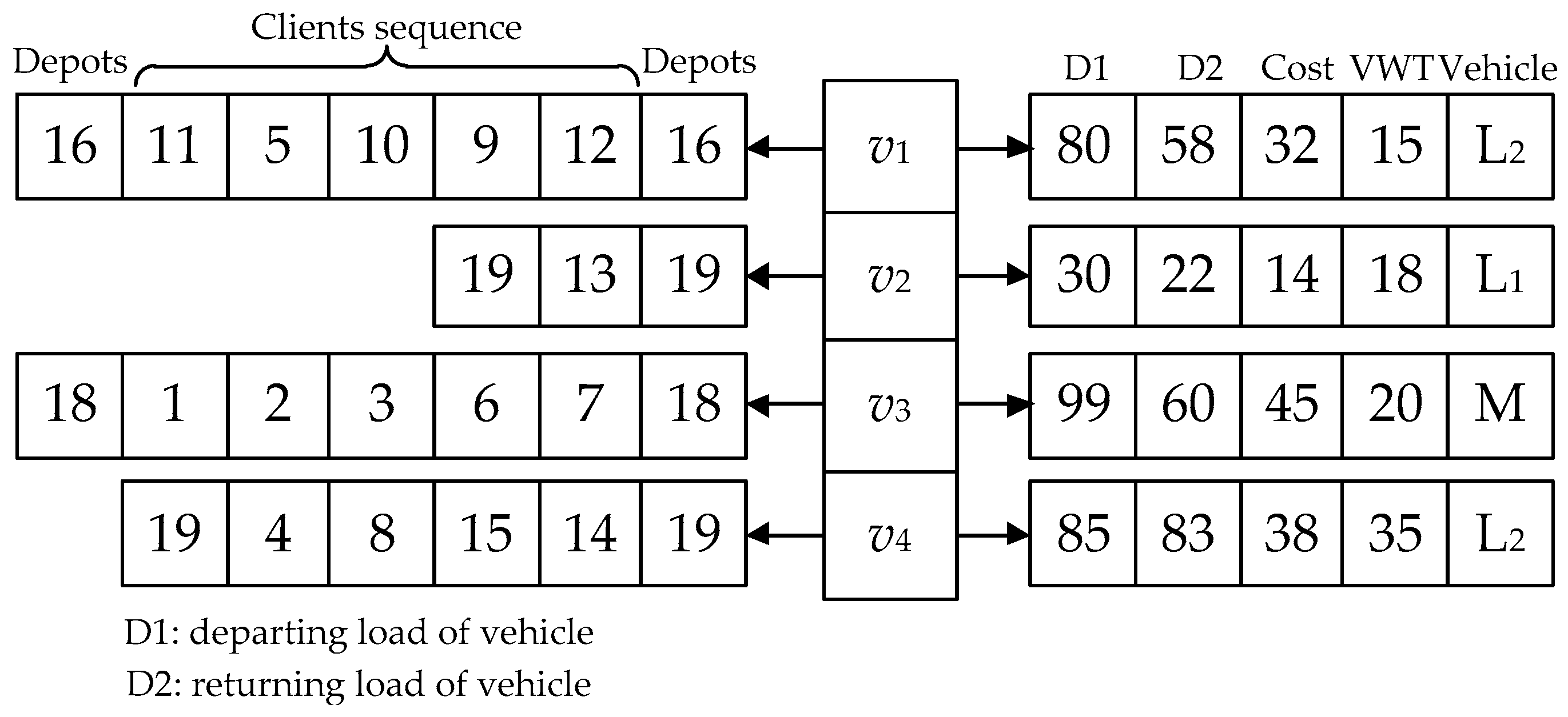
4.1.1. Chromosome Representation

One significant decision in designing a metaheuristic is how to represent and relate the solutions to the search space efficiently [26]. In this paper, we use a simple, intuitive, and competent representation, which was proposed by Leng et al. [6,15] and Zhao et al. [16]. Given the multiobjective problem, we further modified the chromosome representation for the multiobjective RLCLRP. Each solution contains a set of routes, denoted as V = {v1, v2, …, vφ}, where vi is a vehicle traveling route consisting of the service sequence of clients and attributive depot inserted in two ends of it. All routings are kept in a subcell array. It is worth noting that each route must satisfy all constraints (3)–(19) to avoid restoring feasibility for solutions and decoding. To calculate the fitness of each solution quickly, corresponding properties of each route are also stored in its subcell, including the departing and returning loads of the vehicle, the type of vehicle and two objectives concerning cost and vehicle waiting time. The calculation we need to do is to obtain the cost fitness of an individual by simply summing the FCCE, opened depots, and vehicle costs. For the second objective, the vehicle waiting time of each route can be used directly.
To clarify the chromosome representation, Figure 1 provides a simple example of a solution with 15 clients, four depots, and three vehicle types. The left portion shows four vehicle traveling routes, and the right portion shows the properties of each route with the type of vehicle in the last position. All individuals are generated by randomly sorting the sequence of clients and applying a greedy rule to partition clients into sets assigned to each vehicle, and then each route is assigned to the depot that can service those clients in this routing.

4.1.2. Pool of Low-Level Heuristics

In this paper, we focus on MOHH-II by using four efficient MOEAs: SPEA2, NSGA-II, NSLS, and BiGE. A general framework for the RLCLRP is developed as shown in Algorithm 1. Mpop is the mutational population and Cpop is the population after performing local search operators. Line 1 is used to generate the necessary parameters if needed. Lines 2–21 are the iterations for obtaining the Pareto solutions. First, one of the mutation operators is randomly selected to perturb the chosen individual in the population (by tournament, if needed), then the results are merged into Mpop. Then we merge the newly generated solutions with the remaining individuals without mutating into the next phase if the number of mutational individuals is less than N. After that, one of the local search operators is randomly applied to improve each individual in Mpop, and the new population CPop is obtained. Lines 18 and 19 show the basic difference among four MOEAs, as the environmental selection is an extremely significant part of maintaining the trade-off between exploration and exploitation. A stopping criterion is designed as the maximum number of generations, namely maxgen. In the following, it is important to decide how to define the operators. Leng et al. [6] provided 16 domain knowledge operators for the single-objective RLCLRP, and in this paper, we adopt and modify those operators to tackle the multiobjective RLCLRP, as follows.
Algorithm 1. General framework of multi-objective algorithm for LCLRP
Sustainability 11 01596 i001
Among the operators in this paper, three types can be distinguished according to their role in search space: mutational operators (Mu), nondominated local search operators (NDLS), and dominating local search operators (DLS). Among the first ones, although insufficient for achieving competitive results, they are usually helpful for providing randomization in the search for a global optimum by performing simple and slight moves, as follows:
  • Mu 1: Add. Diversifies the selected depots by opening a new one and randomly assigning between one-third and two-thirds of the routes to it [7], or closes one depot and all of its routes are assigned to another depot [6].
  • Mu 2: Decomposition. Routes with vehicles of type L2 and M are randomly (0.5) decomposed into two vehicles with a lower load.
  • Mu 3: Interchange. One-third to two-thirds of routes with at least two clients are randomly selected to swap one client with another.
  • Mu 4: Shift. Shifts a client into any place of another route.
The second module is developed for quickly obtaining nondominated or solution-dominating parent, as follows:
  • NDLS 1: 2-Opt. Exchanges two edges between different routes.
  • NDLS 2: Swap. Swaps one client between different routes.
  • NDLS 3: Swap of a segment. Swaps two or three clients between different routes.
  • NDLS 4: Relocation. Relocates a single client into another route.
  • NDLS 5: Relocation of a segment. Relocates two or three clients into another route.
  • NDLS 6: Decomposition 2. Decomposes all routes with at least two clients into two vehicles.
For DLS, five operators are proposed to obtain better solutions, namely results dominating parent, and the operators are developed by modifying constraints in NDLS 1–5. For the above operators, a key aspect is how to construct the implementation rules. To reduce computing time, we developed a rule whereby, if two groups of routes are obtained by randomly classifying them, then only the routes from the different group can be operated mutually; this rule is implemented in NDLS 1–5, DLS 1–5 and Mu 4. It is worth noting that, as long as restrictions (3)–(19) are satisfied, the moves would be implemented, because no repair methods are needed and computing time is reduced.

4.2. High-Level Control Stratrgy

The HLH of the proposed MOHH framework is developed to select an appropriate heuristic to search the solution space and judge the acceptance of the resultant solutions. In the dynamical search environment, the performance of an LLH in a very early stage may be irrelevant to its current performance. Therefore, the HLH should be capable of quickly and accurately reflecting the performance of each heuristic and choosing the most appreciate LLHs to escape the phase optimal. Resolving this issue entails a design a strategy that can accurately monitor and track the performance of each LLH, that is, the chosen probability of each heuristic should be updated based on its real-time performance. An acceptance criterion in the HLH is used to decide whether or not to accept the resultant solutions. The convergence speed and direction, diversity, and strength of hyper-heuristics, to some extent, are determined by an acceptance criterion. Similarly, the design of an acceptance criterion in the MOHH is a different key technology.

4.2.1. Proposed High-Level Selection Strategy

In quantum computing, quantum bits and the superpositions of states make up the basic concept and principle. Instead of using binary and numeric representation, the qubit chromosome is used as a probabilistic representation and a qubit individual is modeled by a string of qubits.
A qubit is the smallest information storing unit; it may be in the 1 or 0 state, or in any superposition of these, as shown in Equation (28). During the update process, a q-gate is used to change the qubit to a more reasonable state, which is similar to the process of the LLH selected probability. In this paper, we use qubit to represent the LLH selection. Given ζ heuristics, a qubit individual with a string of |ζ| qubits can be expressed as follows:
| ψ = α | 0 + β | 1 ,
L L H = { l l h 1 , l l h 2 , , l l h | ζ | } = [ α 1 α 2 α | ζ | β 1 β 2 β | ζ | ] ,
where llhi = [αi,βi]T is the qubit for the i-th LLH and αi and βi are the complex numbers. The parameters |α|2 (|β|2) are, respectively, the probability that a qubit will be found in the 0 (1) states (i.e., the probability of heuristic disuse (selected) states). Constraints should be secured between α and β, namely, α2 + β2 = 1. Once the beginning of the search, α2 is equivalent to β2, namely, α2 = β2 = 0.5.
The q-gate is an evolutionary learning strategy used to update the state of each qubit of individual and heuristics space, as given in
[ α i t + 1 β i t + 1 ] = [ cos ( μ θ i ) sin ( μ θ i ) sin ( μ θ i ) cos ( μ θ i ) ] × [ α i t β i t ] ,
where μ and θ are, respectively, the rotation direction and angle each qubit towards to 0 or 1 state.
In the following description, we present a strategy for calculating μ and θ by using the D-metric [62,69], which is an extended version of the hypervolume (HV) [62,69] used to measure the covered space between Pareto solutions obtained and a reference point. The description of the D-metric is depicted in Figure 2 [62,69].
In Figure 2, w12 is the space covered by front 1 and not covered by front 2, and w21 represents the size of the space dominated by front 2 and not dominated by front 1. The value γ is the intersection space simultaneously covered by fronts 1 and 2, and the mathematical relations can be provided as
{ w 12 + w 21 + γ = J ( F 1 + F 2 ) w 12 + γ = J ( F 1 ) w 21 + γ = J ( F 2 ) ,
where ϑ(F1 + F2) is the union space covered by fronts 1 and 2 and ϑ(F1) and ϑ(F2) are, respectively, the space covered by fronts 1 and 2. We can further deduce that
{ w 12 = D ( F 1 , F 2 ) = J ( F 1 + F 2 ) J ( F 2 ) w 21 = D ( F 2 , F 1 ) = J ( F 1 + F 2 ) J ( F 1 ) ,
where D(F1, F2) represents w12. As stated by Zitzler [69], if w12 = 0 and w21 > 0, then front 2 dominates front 1. Maashi et al. [62] further slacked the dominance relation: if w21 > w12, then front 2 dominates front 1. Therefore, the former is a strict version of the latter. To use the dominance relation, we determine the rotation direction by the following equation:
μ = { 1 , w 12 < w 21 ± 1 ,   otherwise + 1 , w 12 > w 21 .
If we assume that front 1 is the resultant front and that front 2 is the parent front, after determining the μ, the most significant task is to calculate the rotation angle. In this paper, we use multi-indicators to calculate the reward values, such as the HV, spacing, and nondominated relation. The dominance relation between Fc and Fp can be expressed as
F I R c , p = { 1 ,     if   f c f p 0 ,     if   f c f p 0.5 ,     otherwise
N D V = c F c p F p F I R c , p | F c | × | F p |
R e w a r d ( i ) = N D V × H V S + 1 ,
where fc and fp are, respectively, a child solution of Fc and a parent of Fp; HV and S are, respectively, the hypervolume and spacing value after standardization by dividing the maximum value in the union set of Fc and Fp (which effectively standardizes the magnitude size of HV and S). HV can represent the convergence and distributivity of Fc. S denotes the uniformity of Fc. Therefore,
R e w a r d ( i ) = N D V × H V S + 1
can efficiently describe the characteristics of Fc and provide the performance indicators for LLH. The heuristic qubit associated with LLH performance can then be generated by
θ i = p f ( i ) 1 | ζ | l h ζ p f ( l h ) Q × ( max ( p f ) min ( p f ) + ε )
where pf (lh) is the performance score of the lhth heuristic and Q is a constant ensuring that the θ value range is [–0.05π, 0.05π].
In each iteration, a metaheuristic from a pool of heuristics is chosen by roulette selection for the population. In the roulette selection, the probability of each LLH is
s p ( i ) = β i 2 i ζ β i 2 .
Algorithm 2 calculates the reward, including two aspects involved in the quantum-inspired selection strategy: calculation of the rotation direction and angle. Algorithm 3 is the quantum-inspired learning selection, involving two aspects: a q-gate update process and selection of low-level metaheuristics.
Algorithm 2. Pseudo code of calculating rotation direction and angle
Sustainability 11 01596 i002
Algorithm 3. Quantum-inspired learning selection strategy
Sustainability 11 01596 i003

4.2.2. Proposed High-Level Acceptance Criterion

First, we introduce two acceptance criteria, GDA and LA, which were used in Mashael et al. [62] to solve multiobjective continuous problems (i.e., Walking Fish Group and the crashworthiness test suite). Two significant parameters are involved: Level and S. Level is the water level initially assigned by D(Ppop, Cpop), and S is the prefixed speed rate. According to the GDA rule, the child population with D(Cpop, Ppop) > Level can replace the parent population. Once the child population is accepted, the Level value will be added to S. As the Level increases, a greater difference between child and parent populations is required to accept the child population than previous iterations.
LA is another acceptance criterion using the D-matrix. In the LA mechanism, a list C of length L is used to record D(Cpop, Ppop) and is initialized to D(Ppop, Cpop) at the first iteration. In the acceptance mechanism, if D(Cpop, Ppop) > Cl or D(Cpop, Ppop) > D(Ppop, Cpop) is satisfied, then the resultant solutions are accepted. However, if the above constraints are declined, then Cl is set to the D-matrix of the pair of the front when Ppop was accepted previously. Compared to GDA, LA is the slacker version. Mashael et al. [62] illustrated that GDA is much more efficient than LA. In this paper, we provide another acceptance criterion based on the metaheuristic environmental selection, namely the nondominated sorting and crowded distance of NSGA-II (AC-NDSCD). The major reasons for introducing this criterion are as follows: (i) NSGA-II has been a mainstream MOEA, and the performance of its environmental selection is comparably better than others; and (ii) the proposed acceptance mechanism is irrelevant to domain knowledge (i.e., LCLRP). Unquestionably, many better environmental selections from other MOEAs can be used as the acceptance criterion, but the main idea is to illustrate that environmental selections from MOEAs are also utilized as acceptance mechanisms. Our experimental results show that our proposed AC-NDSCD outperforms GDA and has performance similar to that of LA.

4.3. Framework of the Proposed Hyper-Heuristic

Algorithm 4 is the framework of the quantum-inspired hyper-heuristic, which provides one part outside main loop and four parts insides main loop. The algorithm begins initialization by setting parameters and generating a population made of feasible random chromosomes, stopping when a maximum number of iterations is reached, maxiter.
Algorithm 4. Framework of the Quantum-inspired Hyper-heuristc
Sustainability 11 01596 i004
In each iteration of the main loop, a metaheuristic (MOEA) is chosen by the quantum-inspired selection strategy, then the selected MOEA is applied to generate the child population (Cpop). Finally, the acceptance mechanism is used to maintain exploration and exploitation of Pop into the next iteration by GDA, LA, and AC-NDSCD. Archived methods can also be applied in the proposed algorithm; as Zhang et al. [70] stated, an external approach can always obtain better solutions. In this paper, we save 5 × N archived individuals in each iteration.
The algorithm ends when the main loop stops, returning the Pareto solutions. For the sake of fairness, the archive method is removed when compared with others without the archive approach.

5. Computational Experiments and Analyses

Implementation aspects and evaluations of the proposed mathematical model and hyper-heuristic are presented and discussed in the following sections.

5.1. Implementation Aspects and Configuration of Parameters

The proposed hyper-heuristic was coded in parallel in MATLAB 2018a and results were achieved using a 4.0 GHz Intel Core i7-6700K CPU with 12 GB of RAM and running Windows 10.
The parameters of the proposed hyper-heuristic were obtained empirically. We conducted an empirical evolution with 10 runs for each parameter set in the hyper-heuristic. In this evaluation, we tested different parameter settings to obtain the solutions and found that the following were the most suitable. It is worth noting that we prefer to use the parameter configuration found in the literature.
The maximum iteration (maxiter) was set to 100, and the maximum generation (maxgen) depended directly on the number of clients (N) as follows:
m a x g e n = α × N .
The multiplier α depended on the size of the instance, taking the values 30 for 20 clients, 38 for 30 clients, 45 for 40 clients, and 53 for 50 clients. In other words, the total iterations were 2000 for 20 clients, 3800 for 30 clients, 4500 for 40 clients, and 5300 for 50 clients. The number of individuals in the population and archive population were, respectively, set to 100 and 500.
We also evaluated the range of mutation probability from 0.1 to 0.5. The value was set at 0.35. The reasoning is that the larger the value, the more mutational individuals (Mpop) perform local search, and the more time-consuming it becomes, and the fewer individuals from Ppop there are, the less intensified the search for good solutions, and vice versa.
The configuration parameters used in GDA and LA follow the default values suggested in Maashi et al. [62]: rain speed (S = 0.0003) and list length (L = 5).
We identified the following points that can be threats to the validity of results: (i) The parameter settings may affect the results, as they may change with the characteristics of instances; and (ii) the experiments were conducted using only four datasets (20, 30, 40 and 50 clients) and tested over 10 independent runs, and it is necessary to execute more experiments with a broader range of datasets and larger independent runs to see whether similar behavior is maintained.

5.2. Test Instances

Because instances of the proposed biobjective problem are lacking and the problem is first studied in this paper, the test instances are randomly generated and based on the purposes of the experiments. The logistics distributed field is partitioned into three speed zones (1, 2, and 3) as follows. The speed of each zone was set to Szone1~U(20, 40), Szone2~U(40, 60) and Szone3~U(60, 80) km/h, and the size of each zone was stochastically conducted, and the nested nature was maintained. All clients and depots were located in a 10×10 km2 grid. Three sets of instances were generated: Verification of Efficiency (EFFVER), Locations of Depots, and Clients (LDC), and Large Fleet (LFLEET). The first set was utilized to verify the efficiency of the proposed algorithm (Section 5.4) and the mathematical model (Section 5.5). The second set was used to detect the joint effect of the locations of depots and clients; the last set was used to analyze the effect of fleet composition. Among the above instances, the cost of fuel consumption (cfc) was set to 6.708 RMB/L and the cost of CE (cce) had a value 32.09 RMB/ton. Time windows of the clients were randomly selected from the instance C101 proposed by Solomon et al. [71] and modified by dividing by 10. The service time of each client depends on the total demand (delivery and pickup) and the maximum for all clients was set to 540 s; the pickup and delivery demands of all clients obeyed a uniform distribution in the range 100–2000 kg. The cost of depots in zone 1, zone 2, and zone 3 was, respectively, 500, 300 and 200 RMB. The capacity of each depot also obeys a uniform distribution from in the range [20,25] tons; The cost of fleet composition was set to 38, 44, and 54 RMB for L1, L2, and M, respectively. The cost was used as one-time task instead of for one day, and other parameters were obtained from Koc et al. [1].

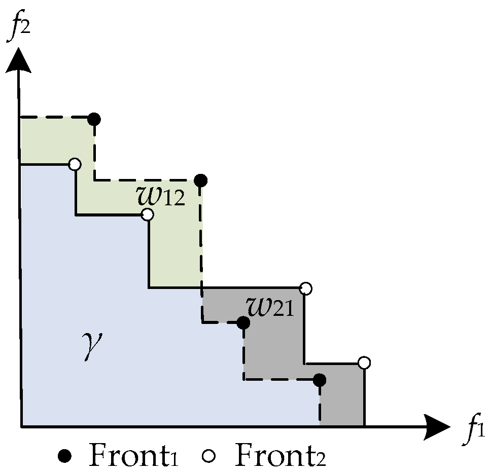
5.3. Performance Metrics

As stated by Li et al. [72], the assessment of a MOEA is mainly entails (i) the proximity to the real Pareto front (PF) (the closer, the better) and (ii) the diversity of solutions (the wider the front is, the better). Taking into account these evaluation criteria, we utilized two widely used metrics to evaluate the convergence, uniformity, and diversity of the approximate front (AF): inverted generational distance (IGD) [62,72,73] and HV [62,69,74].
The IGD value represents the quality and uniformity of AF, and the lower the IGD value, the better the quality and uniformity of AF for approximating the entire PF. Meanwhile, the HV value can express the distribution and diversity of AF, and the larger the HV value, the better the distribution and diversity of AF.
It is worth noting that both IGD and HV are calculated after normalization. Also, in our case, the true Pareto solutions are unknown. For this reason, and following the literature [69,74], PFture was obtained by all approximated Pareto solutions achieved with all methods over 10 runs after removing dominated and repeated solutions, which is, in fact, an approximation of the real front.

5.4. Efficiency of the Proposed Hyper-heuristics

To compare the proposed algorithm with existing MOEAs, we conducted experiments on the four LLHs and another four MOEAs that performed well in solving multiobjective continuous optimization problem: grid-based evolutionary algorithm (GrEA) [75], IBEA [76], NSGA-III [77], and region-based selection in evolutionary-II (PESA-II) [78], which are also the LLHs of MOHH/QS2. The results of the 10 approaches are provided in Table 1 and Table 2, which show the mean IGD (Table 1) and HV (Table 2) values obtained by performing 10 runs, where the last row is the number of first, second, and third places in each instance, abbreviated as f/s/t. In each table, the last two columns provide the results obtained by MOHH/QS and MOHH/QS2, and the former used BiGE, NSGA-II, NSLS, and SPEA2 as LLHs.
From Table 1, we find that MOHH/QS obtained 13 best mean IGD values in 16 instances and three third places, while MOHH/QS2 obtained only one best mean IGD value, three second places, and one third place. SPEA2, NSLS, NSGA-II, and BiGE are the top in eight MOEAs, while the other four MOEAs obtained only a few beneficial results. From Table 2, we see that MOHH/QS obtained nine best mean HV values, four second places, and two third places, and MOHH/QS2 also performed well by obtaining five best mean HV values, four second places, and two third places. NSGA-II, SPEA2, IBEA, and NSGA-III performed better than others in terms of the total number of places in each instance.
The following conclusions can be drawn from the results in Table 1 and Table 2: (i) A combination of MOEAs can efficiently improve their performance, as both MOHH/QS and MOHH/QS2 outperformed the others in both mean IGD and HV values; (ii) LLHs have a huge impact on the performance of methods even though they shared the same high-level strategy (QS+GDA), because MOHH/QS outperformed MOHH/QS2; therefore, testers should select some outstanding operators as LLHs to improve their algorithm’s performance; and (iii) the proposed MOHH method is meaningful for solving the proposed problems. Given the performance of SPEA2, NSLS, NSGA-II, and BiGE, the following experiments were tackled by using MOHH with the above metaheuristics as LLHs.

5.5. Efficiency of Nine Pairs in MOHH

In this section, we compare nine pairs developed in MOHH; in other words, the SR, FRR-MAB (FM), CF, and QS are selected as the high-level selection strategies and GDA, LA, and AC-NDSCD are utilized as the high-level acceptance criteria. The EFFVER set is also used as instances to evaluate the performance of each pair, and the results obtained for the nine pairs are given in Table 3 and Table 4.
Looking at Table 3, QS/LA achieves five best mean IGD values, four second places, and two third places, and QS/AC-NDSCD performs well in 16 instances by achieving three best mean IGD values, five second places, and two third places. These two proposed approaches are the best two algorithms. For the third version of the proposed selection strategy, QS/GDA seems to be better than FM/GDA and worse than SR/GDA and CF/GDA. For all versions applying LA, QS/LA was the best one among SR/LA, FM/LA, and CF/LA. For the versions applying QS, QS/LA was also the best, and QS/AC-NDSCD was in the second place (which is also the second place in nine pairs), and QS/GDA was the worst among the three versions. However, the above conclusion on QS/LA and QS/AC-NDSCD seems to differ in Table 4, as the first place in nine pairs is QS/AC-NDSCD instead of QS/LA, and QS/LA is the second place in nine pairs. Meanwhile, the third version of QS (QS/GDA) also performed well in nine pairs and was better than all variants of GDA. For versions of QS, AC-NDSCD performed the best, and QS/LA was better than QS/GDA.
Therefore, the following conclusions can be made: (i) the selection strategy is one of the most significant parts in hyper-heuristics, and different selection strategies can, more or less, improve performance, but a poor selection strategy can pull down the performance of algorithms. The proposed selection strategy outperforms the others (SR, FM, and CF) combined with GDA and LA (except for QS/GDA in mean IGD values); and (ii) the acceptance criterion is also one of the most important components; both LA and AC-NDSCD perform well in most instances and were better than GDA, which was different from the conclusion of Maashi et al. [62]. Therefore, the environmental selections are also the alternative acceptance criteria in the framework of hyper-heuristics. In the following experiments, we randomly selected one of the acceptance criteria (LA and AC-NDSCD) and utilized QS as the selection strategy.

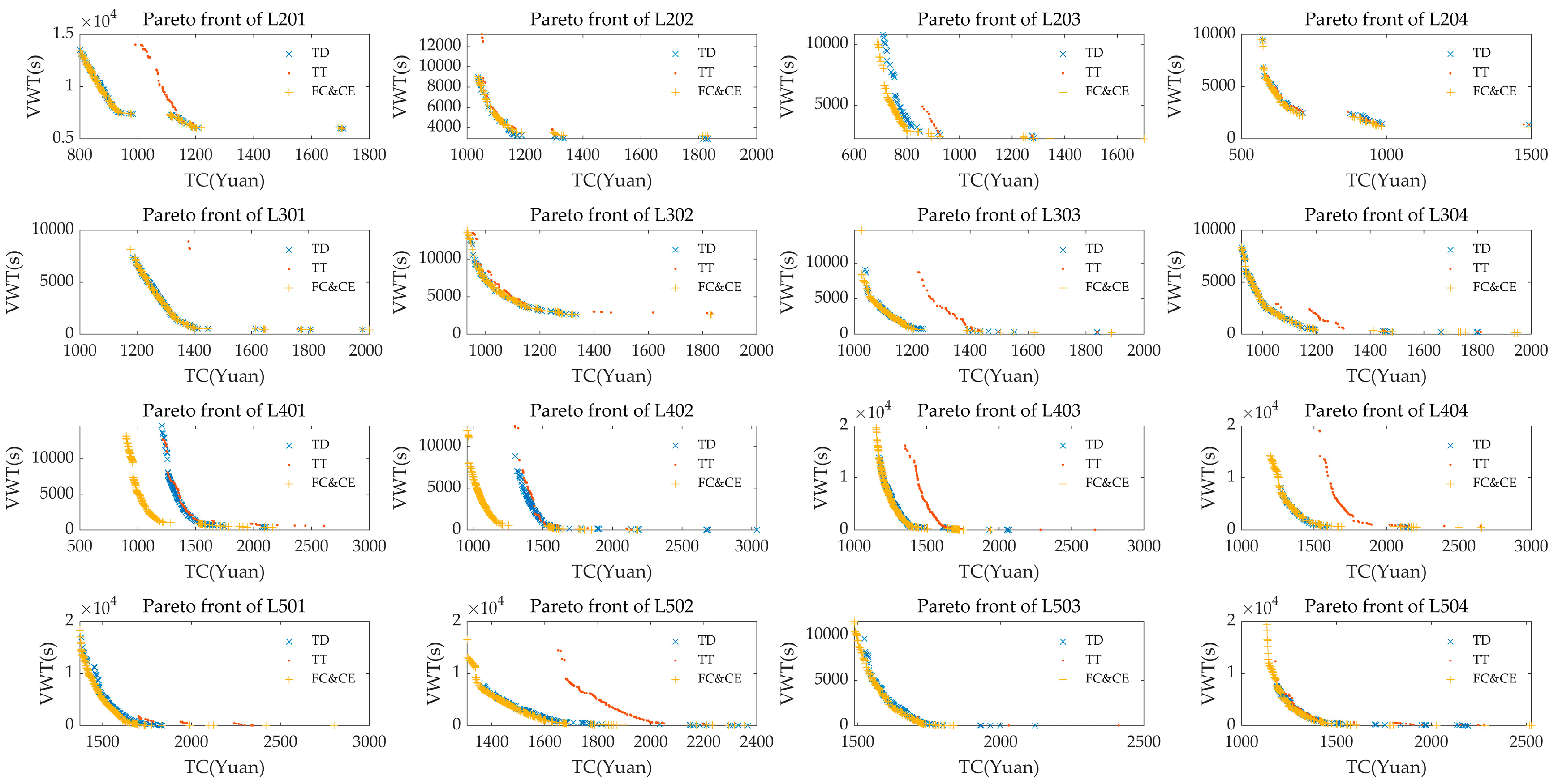
5.6. Efficiency of the Proposed Mathematical Model

This section provides an evaluation of the efficiency of the proposed model by comparing the Pareto front of three models: RLCLRP/FCCE, RLCLRP/TD, and RLCLRP/TT. The first applies FCCE cost as the travel cost, while the second uses travel distance (TD) in kilometers as the travel cost, and the last one utilizes the travel time (TT) in minutes as the travel cost. To compare the Pareto front of each model, Pareto solutions of RLCLRP/TD and RLCLRP/TT were recalculated in the context of RLCLRP/FCCE to obtain comparable Pareto solutions; in other words, the proposed model was used to calculate the total cost (TC) and vehicle waiting time (VWT) for Pareto solutions obtained by RLCLRP/TD and RLCLRP/TT. The test instances were the same as the above set (EFFVER), and the mean IGD and HV values are listed in Table 5.
Looking at Table 5, the Pareto solutions of RLCLRP/FCCE dominate all Pareto solutions obtained by RLCLRP/TD and RLCLRP/TT in L20-3, L30-1, L30-2, L30-4, L40-2, and L50-1, and dominate most Pareto solutions obtained by RLCLRP/TD and RLCLRP/TT in other instances. Meanwhile, the mean IGD values of RLCLRP/FCCE are the smallest in each instance and are, respectively, reduced by 97.69% and 98.91% on average when compared with the mean IGD values obtained by RLCLRP/TD and RLCLRP/TT. The mean HV values of RLCLRP/FCCE are the largest for each instance (except for L20-2) and are, respectively, increased by 4.98% and 22.38% on average when compared with the mean HV values of RLCLRP/TD and RLCLRP/TT.
A question that arises when comparing the results of the three models is “why does the Pareto front of RLCLRP/FCCE not dominate all Pareto solutions of the other two in all instances?” Two of the principal reasons can be expressed as follows. The first is problem domain nature, namely clients’ time windows. The rules of RLCLRP/TD and RLCLRP/TT use the minimum TD and TT to guide the vehicles to service clients instead of FCCE, and the result is that traveling time may differ from that of FCCE, and some clients may be not satisfied for RLCLRP/FCCE even if all three share the same routes. For example, a route v = {21,1,2,3,21} can be finished by models of the latter two but may not be met by RLCLRP/FCCE, because RLCLRP/FCCE selects the nondominated routes (travel distance and FCCE) [1], resulting in different travel times. Then, the second is that efficiency of the proposed algorithm is barely satisfactory to optimize true Pareto fronts of RLCLRP/FCCE. However, in our experience with optimization, the first explanation is the main issue.
Figure 3 shows the Pareto fronts of the three models for tackling the EFFVER set. Most solutions of RLCLRP/TD and RLCLRP/TT are dominated by the Pareto fronts of RLCLRP/FCCE, although a few solutions coincide with those of RLCLRP/TD. Furthermore, it is undeniable that our proposed model is more suitable and better than RLCLRP/TD and RLCLRP/TT in addressing sustainable economy, society, and environment.

5.7. Evaluation of the Effect of the Domain Problem

In this section, we evaluate the effects of domain parameters (i.e., fleet composition and distribution of clients and depots) on TC, VWT, opening depot, assigned vehicle, FCCE cost, FC, CE, TD, and TT. Section 5.7.1 analyzes the joint effect of variations in depots and client locations, and Section 5.7.2 evaluates the effect of fleet composition.

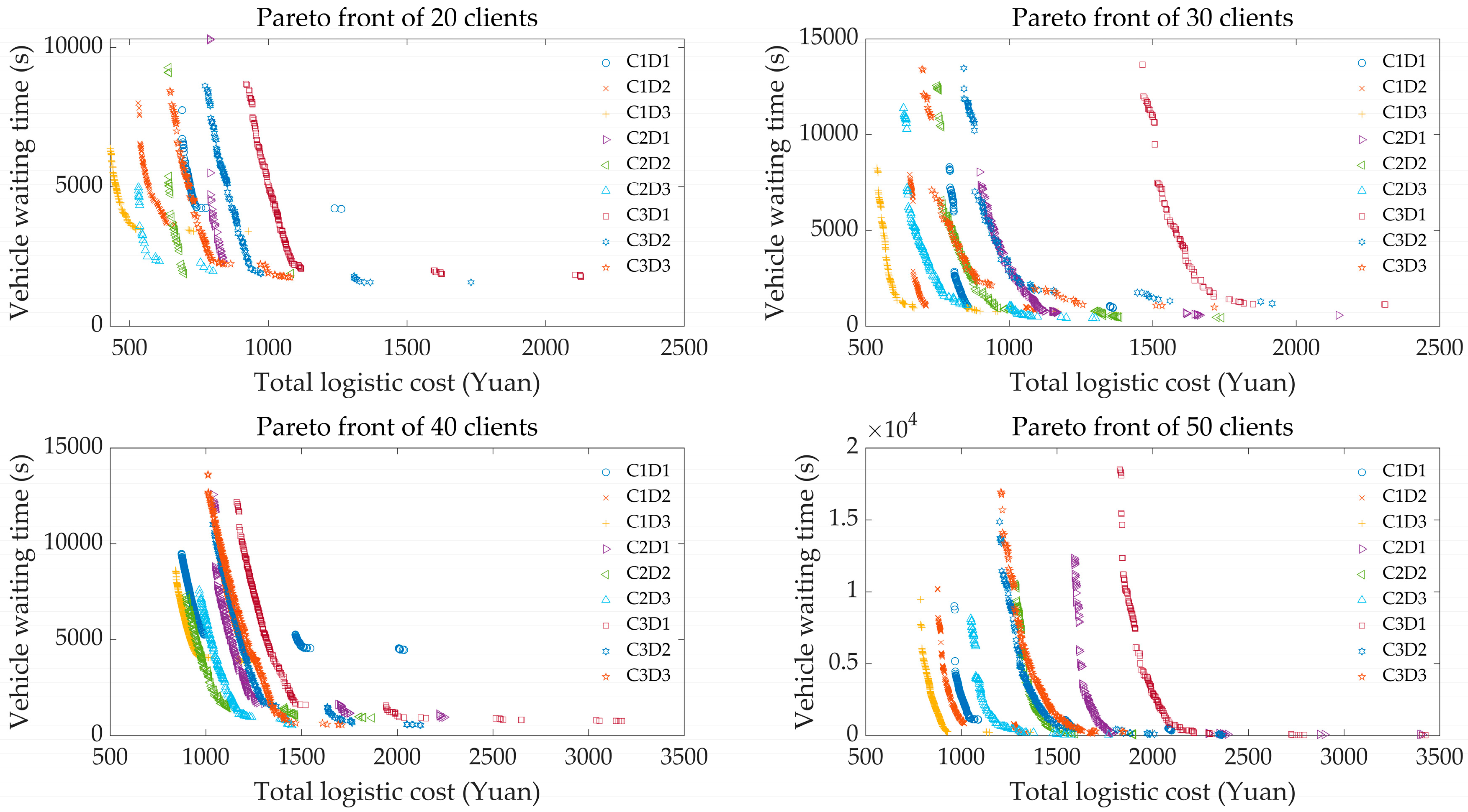
5.7.1. Joint Effect of Depots and Client Distribution

As discussed above, three zones are partitioned, and a different speed is assigned to each zone. Therefore, the distribution of clients and depots may be one of the most significant factors affecting the key performance indicators of logistics networks. To solve this problem, we conducted a series of experiments to evaluate the joint effect of the distribution of clients and depots, as shown as in Figure 4, where CnDm is the representation of clients and depots distribution; C and D, respectively, represented clients and depots, and n and m, respectively, represent locations of clients and depots, with n, m∈{1,2,3}.
Figure 4 shows that Pareto solutions of C1D3 can dominate the majority of other Pareto solutions, especially when TC is small. In the fronts of 20 clients, the dominating sequence is C1D3 ≺ C2D3 ≺ C2D2 ≺ C3D3 ≺ C1D2 ≺ C3D2 ≺ C2D1 ≺ C1D1 ≺ C3D1. In the fronts of 30 clients, the dominating sequence is C1D3 ≺ C2D3 ≺ C1D2 ≺ C2D2 ≺ C1D1 ≺ C3D3 ≺ C2D1 ≺ C3D2 ≺ C3D1. In the fronts of 40 clients, the dominating order is C2D2 ≺ C1D3 ≺ C2D3 ≺ C1D1 ≺ C2D1 ≺ C3D2 ≺ C3D3 ≺ C1D2 ≺ C3D1. In the fronts of 50 clients, the dominating order is C1D3 ≺ C1D2 ≺ C1D1 ≺ C2D3 ≺ C2D2 ≺ C3D2 ≺ C3D3 ≺ C2D1 ≺ C3D1. In Figure 5, the circled numbers indicate number of the clients’ locations in the zone, and the number in squares is number of the depots’ locations in the zone; for example, the first is the preference of 20 clients for depots in each zone, and the clients in Zone 1 prefer the depots in Zone 3 instead of those in Zone 1. Although the distance between clients and depots in Zone 1 is less than for others, as long as all clients’ time windows are satisfied, the depots in Zone 3 are an optimal choice. The second is the preference of depots in each zone according to the zone’s clients. For example, depots in Zone 1 are asked to service 20 clients, and clients in Zone 2 are the best choice for them, instead of clients in Zone 1, and clients in Zone 1 should be serviced by depots in Zone 3. Moreover, clients in Zone 3 should be serviced by depots in Zone 3, as a sequence of dominant symbol (A ≺ B, A dominates B). However, as the number of clients increases, the corresponding preference should be adaptively changed to obtain the best Pareto solutions. Therefore, the joint effect of the locations of both client and depot should be considered simultaneously.
Figure 6 analyzes the ratio of each part in terms of TC: depot, vehicle, and FCCE costs for each instance in LDC; and TD and TT are also calculated to detect whether or not they are affected by the distribution of depots and clients. The ratio of depot cost decreases as TC increases at the beginning for all nine pairs and {20,30,40,50} clients, indicating that Pareto solutions in this part are variations sharing the same set of depots; then the ratio of depot cost increases because new depots are added to the set of depots, but the ratio of fleet and FCCE cost decrease in the second and third columns. Fleet cost decreases as TC increases for all nine pairs and {20,30,40,50} clients, illustrating that fleet composition stays the same under all conditions, and fleet composition depends on the pickup and delivery demand and clients’ time windows instead of the distribution of depots and clients, which can be explained by the following: TC increases with FCCE cost at the beginning, and continued decline is caused by adding new depots to the set of depots. Surprisingly, FCCE cost increases with TC at the beginning, while the ratio of depot cost and fleet cost decreases, which indicates that the increment of FCCE cost is the main reason for the increased TC because Pareto solutions in this part share the same depot set and fleet composition. However, if the set of depots is expanded by adding new depots, the FCCE cost keeps increasing, which demonstrates that adding new depots may not help reduce the FCCE cost in the context of a fixed set of depots. For TD, similar characteristics can be found in FCCE cost, indicating that a positive correlation exists between FCCE and TD, which explains some of the overlapping results exist in Figure 3. For TT, there seems to be no relationship with the distribution of clients and depots, as the biobjectives of the proposed problem are total cost and vehicle waiting time.
Therefore, from Figure 6, we see that speed zones have some influence on the performance indicators as indicators of each pair are different from those of others. Government and logistic enterprises may impose various rules on logistics network to optimize corresponding indicators for ameliorate the economic, social, and environmental effect.

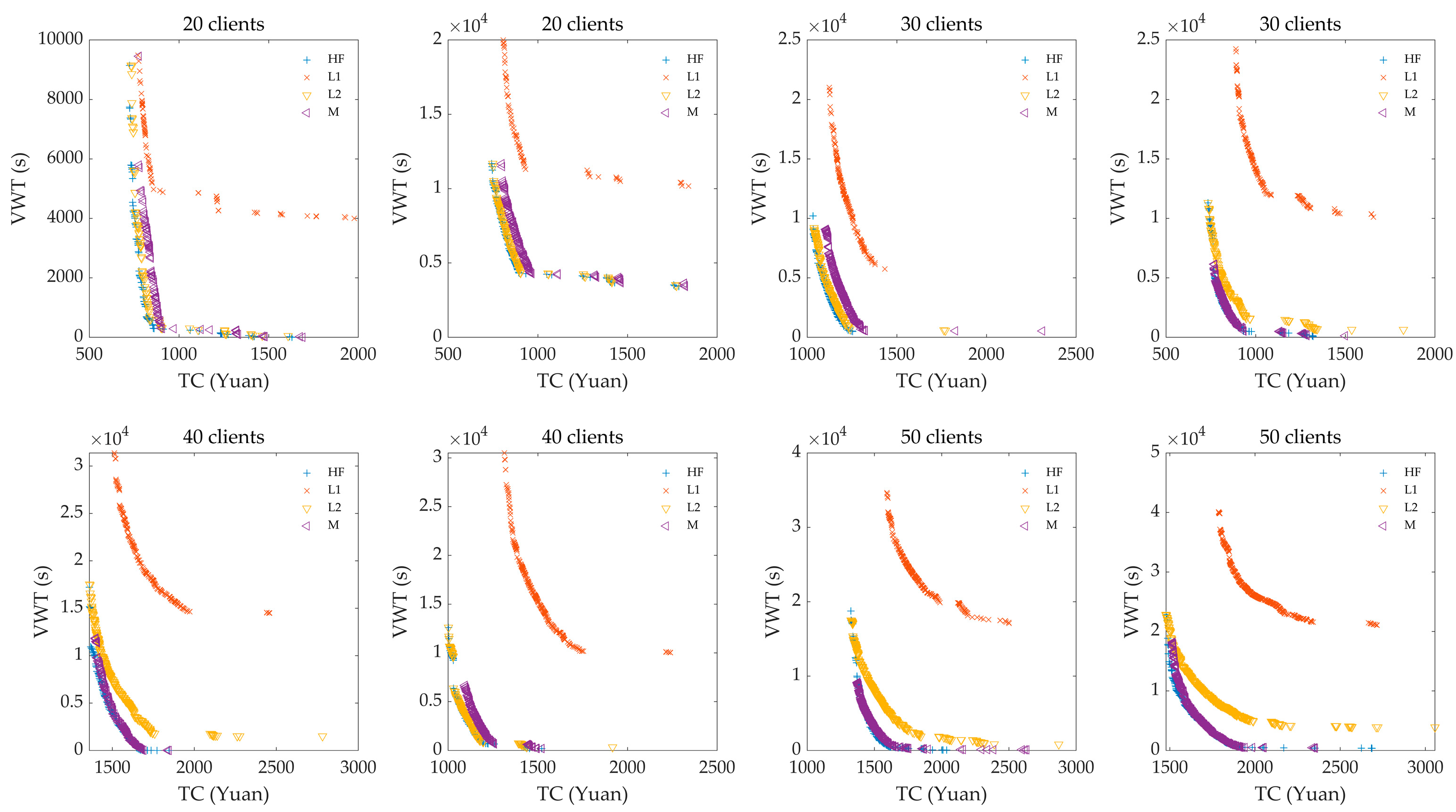
5.7.2. Effect of Fleet Composition

The purpose of this section is to test the effect of fleet composition on the pivotal performance indicators of the logistics network. In the generated LFLEET suite, eight instances are used, and the results are listed in Table 6. In all instances, IGD values are equal to zero, and mean HV values are greater than those of others, indicating that Pareto solutions of HF dominate all Pareto solutions of others. Figure 7 presents the Pareto front of each instance with different fleet composition. In cases of 20, 30, and 40 clients, the vehicle type L2 seems to be preferably selected. However, the vehicle type M is preferred in the context of larger cases with 30, 40 and 50 clients. Meanwhile, the fleet of type L1 may be abandoned in all instances. Therefore, logistics enterprises should rent or purchase vehicles of types L2 and M.
Figure 8 shows the effect of fleet composition on the key performance indicators: ratio of FCCE cost, CE in kilograms (or FC in Liters), TD, and TT. A conclusion can be reached: the fleet with HF can help effectively reduce the TC, VWT, FCCE cost, CE (FC), TD, and TT.
The results of this section indicate that the proposed algorithm can solve the problem effectively and outperforms other customized MOEAs and that the proposed model is more effective than the models of travel distance and time. Moreover, we also evaluated the effects of domain parameters on several performance indicators of the logistics network and provided some advice from managerial insight.

6. Conclusions

This paper concerned a variant of the location-routing problem, namely, the regional low-carbon location-routing problem considering a city in which goods need to be picked up and delivered from depots to clients located in nested zones characterized by different speed limits. Several real-world conditions were also taken into consideration: simultaneous pickup and delivery, hard time windows, and a heterogeneous fleet. To solve the proposed problem, a biobjective model was developed by viewing total logistics cost as the primary objective and vehicle waiting time as the secondary objective. The total logistics cost consists of three parts: depots cost, vehicles cost, and travel cost, with the latter defined as FCCE cost. A novel approach was designed to tackle the proposed problem: a quantum-inspired hyper-heuristic.
Extensively experiments were performed to (1) verify the efficiency of the proposed algorithm and model and (2) analyze the effects of domain parameters on the key performance indicators. The results show that our algorithm and model are efficient, providing the best results compared to other algorithms and models for benchmark instances. We also analyzed the effects of the domain parameters, such as depot cost and location, client distribution, and fleet composition, on the significant performance indicators, such as total logistic cost, vehicle waiting time, opened depot cost, fleet cost, fuel consumption and carbon emission cost, travel distance, and travel time. Moreover, several constructive suggestions are deduced from simulations to promote the sustainable development of the economy, society, and the environment.
Future works will explore new versions of the RLCLRP that merge the temporal dimension in traffic congestion, and other efficient estimations of fuel consumption and carbon emission will be considered. Additional novel selection strategies and acceptance criteria may also be developed.

Author Contributions

L.L. came up with the main idea of model and algorithm and carried out the simulations. Y.Z. helped with the structure and revisions of the paper. Z.W. and J.Z. investigated the state-of-the-art literature and pointed out some suggestions about literature review; W.W. given some advice about algorithm, coding and results analyses; Z.C. provided some advices about revision.

Funding

This research was funded by the National Natural Science Foundation of China grant numbers 61572438, 61873240, 61402409, National Natural Science Foundation of Zhejiang grant number Y19F030052 and Science Technology plan project of Zhejiang grant number 2017C33224.

Acknowledgments

The authors would like to express our sincere thanks to Yu, V.F. and Lin, S.Y. for their time and patience devoted to the advice and assistance of this paper.

Conflicts of Interest

The authors declare no conflict of interest.

References

  1. Koc, C.; Bektas, T.; Jabali, O.; Laporte, G. The impact of depot location, fleet composition and routing on emission in city logistics. Transp. Res. Part B Methodol. 2016, 84, 81–102. [Google Scholar] [CrossRef]
  2. Bayram, H.; Şahin, R. A new simulated annealing approach for travelling salesman problem. Math. Comput. Appl. 2013, 18, 313–322. [Google Scholar] [CrossRef]
  3. Zhao, Y.; Leng, L.; Qian, Z.; Wang, W. A discrete hybrid invasive weed optimization algorithm for the capacitated vehicle routing problem. In Proceedings of the 4th International Conference on Information Technology and Quantitative Management (ITQM)-Promoting Business Analytics and Quantitative Management of Technology, Asan, Korea, 16–18 August 2016; Lee, H., Lee, J., Cordova, F., Dzitac, I., Kou, G., Li, J., Eds.; Elsevier B.V.: Amsterdam, The Netherlands, 2016; Volume 91, pp. 978–987. [Google Scholar] [CrossRef]
  4. Zhou, L.; Wang, X.; Ni, L.; Lin, Y. Location-routing problem with simultaneous home delivery and customer’s pickup for city distribution of online shopping purchases. Sustainability 2016, 8, 828. [Google Scholar] [CrossRef]
  5. Zhang, C.; Zhao, Y.; Zhang, J.; Leng, L.; Wang, H. Location and routing problem with minimizing carbon. Comp. Integr. Manuf. Syst. 2017, 23, 2768–2777. [Google Scholar] [CrossRef]
  6. Leng, L.; Zhao, Y.; Wang, Z.; Wang, H.; Zhang, J. Shared mechanism-based self-adaptive hyperheuristic for regional low-carbon location-routing problem with time windows. Math. Probl. Eng. 2018, 8987402. [Google Scholar] [CrossRef]
  7. Lopes, R.B.; Ferreria, C.; Santos, B.S. A simple and effective algorithm for the capacitated location-routing problem. Comput. Oper. Res. 2016, 70, 155–162. [Google Scholar] [CrossRef]
  8. Bektas, T.; Laporte, G. The pollution-routing problem. Transp. Res. Part. B Methodol. 2011, 45, 1232–1250. [Google Scholar] [CrossRef]
  9. Liu, X.H.; Shan, M.Y.; Zhang, R.L.; Zhang, L.R. Green vehicle routing optimization based on carbon emission and multiobjective hybrid quantum immune algorithm. Math. Probl. Eng. 2018. Article ID 8961505. [Google Scholar] [CrossRef]
  10. Liu, Y.; Peng, D. Consumption-aware model for eco-routing in vehicle network. J. Chin. Comput. Syst. 2017, 7, 1512–1517. [Google Scholar]
  11. Lin, C.H.; Choy, K.L.; Ho, G.T.S.; Chung, S.H.; Lam, H.Y. Survey of green vehicle routing problem: Past and future trends. Expert Syst. Appl. 2014, 41, 1118–1138. [Google Scholar] [CrossRef]
  12. Demir, E.; Bektas, T.; Laporte, G. A comparative analysis of several vehicle emission models for road freight transportation. Transp. Res. Part D Transp. Environ. 2011, 16, 347–357. [Google Scholar] [CrossRef]
  13. Demir, E.; Bektas, T.; Laporte, G. A review of recent research on green road freight transportation. Eur. J. Oper. Res. 2014, 237, 775–793. [Google Scholar] [CrossRef]
  14. Xiao, Y.Y.; Zhao, Q.H.; Falu, I. Development of a fuel consumption optimization model for the capacitated vehicle routing problem. Comput. Oper. Res. 2012, 39, 1419–1431. [Google Scholar] [CrossRef]
  15. Leng, L.; Zhao, Y.; Zhang, C.; Wang, S. Quantum-inspired hyper-heuristics for low-carbon location-routing problem with simultaneous pickup and delivery. Comp. Integr. Manuf. Syst. 2018, in press. [Google Scholar]
  16. Zhao, Y.; Leng, L.; Wang, S.; Zhang, C. Evolutionary hyper-heuristics for low-carbon location-routing problem with heterogeneous fleet. Cont. Decis. 2018. [Google Scholar] [CrossRef]
  17. Wang, S.; Zhao, Y.; Leng, L.; Zhang, C. Research on low carbon location routing problem based on evolutionary hyper-heuristic algorithm of ant colony selection mechanism. Comp. Integr. Manuf. Syst. 2018, in press. [Google Scholar]
  18. Tang, J.; Ji, S.; Jiang, L. The design of a sustainable location-routing-inventory model considering consumer environmental behavior. Sustainability 2016, 8, 211. [Google Scholar] [CrossRef]
  19. Hwang, T.; Ouyang, Y. Urban freight truck routing under stochastic congestion and emission considerations. Sustainability 2015, 7, 6610–6625. [Google Scholar] [CrossRef]
  20. Jovicic, N.; Boskovic, G.; Vujic, G.; Jovicia, G.R.; Despotovic, M.Z.; Milovanovic, D.M.; Gordic, D.R. Route optimization to increase energy efficiency and reduce fuel consumption of communal vehicles. Therm. Sci. 2010, 14, 67–78. [Google Scholar] [CrossRef]
  21. Liu, W.Y.; Lin, C.C.; Tsao, Y.S.; Wang, Q. Minimizing the carbon footprint for the time-dependent heterogeneous-fleet vehicle routing problem with alternative paths. Sustainability 2014, 6, 4658–4684. [Google Scholar] [CrossRef]
  22. Koc, C.; Bektas, T.; Jabali, O. The fleet size and mix pollution-routing problem. Transp. Res. Part B Methodol. 2014, 70, 239–254. [Google Scholar] [CrossRef]
  23. Bandeira, J.; Carvalho, D.O.; Khattak, A.J.; Rouphail, N.M.; Coelho, M.C. A comparative empirical analysis of eco-friendly routes during peak and off-peak hours. In Proceedings of the Transportation Research Board 91st Annual Meeting, Washington, DC, USA, 22–26 January 2012. [Google Scholar]
  24. Bandeira, J.; Carvalho, D.O.; Khattak, A.J.; Rouphail, N.M.; Coelho, M.C. Generating emissions information for route selection: Experimental monitoring and routes characterization. J. Intell. Transp. Syst. 2013, 17, 3–17. [Google Scholar] [CrossRef]
  25. Chen, C.; Qiu, R.; Hu, X. The location-routing problem with full truckloads in low-carbon supply chain network designing. Math. Probl. Eng. 2018, 6315631. [Google Scholar] [CrossRef]
  26. Mohammadi, M.; Razmi, J.; Tavakkoli-Moghaddam, R. Multi-objective invasive weed optimization for stochastic green hub location routing problem with simultaneous pick-ups and deliveries. Econ. Comput. Econ. Cybern. Stud. 2013, 47, 247–266. [Google Scholar]
  27. Govindan, K.; Jafarian, A.; Khodaverdi, R.; Devika, K. Two-echelon multiple-vehicle location–routing problem with time windows for optimization of sustainable supply chain network of perishable food. Int. J. Prod. Econ. 2014, 152, 9–28. [Google Scholar] [CrossRef]
  28. Validi, S.; Bhattacharya, A.; Byrne, P.J. Integrated low-carbon distribution system for the demand side of a product distribution supply chain: A DoE-guided MOPSO optimizer-based solution approach. Int. J. Prod. Res. 2014, 52, 3074–3096. [Google Scholar] [CrossRef]
  29. Validi, S.; Bhattacharya, A.; Byrne, P.J. A case analysis of a sustainable food supply chain distribution system-a multi-objective approach. Int. J. Prod. Econ. 2014, 152, 71–87. [Google Scholar] [CrossRef]
  30. Qazvini, Z.E.; Amalnick, M.S.; Mina, H. A green multi-depot location routing model with split-delivery and time window. Int. J. Manag. Concepts Philos. 2016, 9, 271–282. [Google Scholar] [CrossRef]
  31. Toro, E.M.; France, J.F.; Echeverri, M.G.; Guimarães, F. A multi-objective model for the green capacitated location-routing problem considering environmental impact. Comput. Ind. Eng. 2017, 110, 114–125. [Google Scholar] [CrossRef]
  32. Nakhjirkan, S.; Rafiei, F.M. An integrated multi-echelon supply chain network design considering stochastic demand: A genetic algorithm-based solution. Promet Traffic Transp. 2017, 4, 391–400. [Google Scholar] [CrossRef]
  33. Wang, Y.; Tian, X.; Liu, D. Optimization of urban multi-level logistics distribution network based on the perspective of low carbon. In Proceedings of the 2017 Chinese Automation Congress (CAC), Jinan, China, 20–22 October 2017. [Google Scholar] [CrossRef]
  34. Wang, X.; Li, X. Carbon reduction in the location routing problem with heterogeneous fleet, simultaneous pickup-delivery and time windows. In Proceedings of the 21st International Conference on Knowledge-Based and Intelligent Information and Engineering Systems (KES), Marseille, France, 6–8 September 2017; ZanniMerk, C., Frydman, C., Toro, C., Hicks, Y., Howlett, R.J., Jain, L.C., Eds.; Elsevier B.V.: Amsterdam, The Netherlands, 2017; Volume 112, pp. 1131–1140. [Google Scholar] [CrossRef]
  35. Rabbani, M.; Davoudkhani, M.; Farrokhi-Asi, H. A new multi-objective green location routing problem with heterogonous fleet of vehicles and fuel constraint. Int. J. Strateg. Decis. Sci. 2017, 8, 99–119. [Google Scholar] [CrossRef]
  36. Wang, S.; Tao, F.; Shi, Y. Optimization of location–routing problem for cold chain logistics considering carbon footprint. Int. J. Environ. Res. Public Health 2018, 15, 86. [Google Scholar] [CrossRef]
  37. Qian, Z.; Zhao, Y.; Wang, S.; Leng, L.; Wang, W. A hyper heuristic algorithm for low carbon location routing problem. In Proceedings of the Advances in Neural Networks-ISNN 2018, 15th International Symposium on NeuralNetworks, Minsk, Belarus, 25–28 June 2018. [Google Scholar] [CrossRef]
  38. Faraji, F.; Afshar-Nadjafi, B. A bi-objective green location-routing model and solving problem using a hybrid metaheuristic algorithm. Int. J. Logist. Syst. Manag. 2018, 30, 366–385. [Google Scholar] [CrossRef]
  39. Walker, J.D.; Ocha, G.; Gendreau, M.; Burke, E.K. Vehicle routing and adaptive iterated local search within the HyFlex hyper-heuristic framework. In Proceedings of the Learning and Intelligent Optimization 6th International Conference, Paris, France, 16–20 January 2012. [Google Scholar] [CrossRef]
  40. Denzinger, J.; Fuchs, M.; Fuchs, M. High performance ATP systems by combining several AI methods. In Proceedings of the International Joint Conference on Artificial Intelligence, Nagoya, Japan, 23–29 August 1997. [Google Scholar]
  41. Cowling, P.; Kendall, G.; Soubeiga, E. A hyper-heuristic approach to scheduling a sales summit. In Proceedings of the International Conference on the Practice and Theory of Automated Timetabling, Konstanz, Germany, 16–18 August 2000; Burke, E., Erben, W., Eds.; Springer: Berlin, Germany, 2000. [Google Scholar] [CrossRef]
  42. Wolper, D.H.; Macready, W.G. No free lunch theorems for optimization. IEEE Trans. Evol. Comput. 1997, 1, 67–82. [Google Scholar] [CrossRef]
  43. Burke, E.K.; Gendreau, M.; Hyde, M.; Kendall, G.; Ochoa, G.; Qu, R. Hyper-heuristics: A survey of the state of the art. J. Oper. Res. Soc. 2013, 64, 1695–1724. [Google Scholar] [CrossRef]
  44. Kalender, M.; Kheiri, A.; Ozcan, E.; Burke, E.K. A greedy gradient-simulated annealing selection hyper-heuristic. Soft Comput. 2013, 17, 2279–2292. [Google Scholar] [CrossRef]
  45. Ozcan, E.; Bilgin, B.; Kormaz, E.E. A comprehensive analysis of hyper-heuristics. Intell. Data Anal. 2008, 12, 3–23. [Google Scholar] [CrossRef]
  46. Sabar, N.; Ayob, M.; Kendall, G. The automatic design of a hyper-heuristic framework with gene expression programming for combinatorial optimization problems. IEEE Trans. Evol. Comput. 2015, 19, 309–325. [Google Scholar] [CrossRef]
  47. Burke, E.K.; Hyde, M.; Kendall, G.; Ochoa, G.; Ozcan, E.; Woodard, J.R. A classification of hyper-heuristic approaches. In Handbook of Metaheuristics; International Series in Operations Research & Management Science; Springer: Boston, MA, USA, 2010; Volume 146, pp. 449–468. [Google Scholar]
  48. Li, K.; Fialho, A.; Kwong, S.; Zhang, Q. Adaptive operator selection with bandits for a multiobjective evolutionary algorithm based on decomposition. IEEE Trans. Evol. Comput. 2014, 18, 114–130. [Google Scholar] [CrossRef]
  49. Nareyek, A. Choosing search heuristics by non-stationary reinforcement learning. In Proceedings of the 4th Metaheuristics International Conference, Oporto, Portugal, 16–20 July 2001; Resende, M.G.C., DeSousa, J.P., Eds.; Kluwer Academic Publishers: Norwell, MA, USA, 2004. [Google Scholar] [CrossRef]
  50. Anagnostopoulos, K.P.; Koulinas, G.K. A genetic algorithm hyperheuristic algorithm for the resource constrained project scheduling problem. In Proceedings of the 2010 IEEE Congress on Evolutionary Computation, Barcelona, Spain, 18–23 July 2010. [Google Scholar] [CrossRef]
  51. Chen, S.; Li, Z.; Yang, B.; Rudolph, G. Quantum-inspired hyper-heuristics for energy-aware scheduling on heterogeneous computing systems. IEEE Trans. Parallel Distrib. Syst. 2016, 27, 1796–1810. [Google Scholar] [CrossRef]
  52. Dueck, G. New optimization heuristics: The great deluge algorithm and the record to record travel. J. Comput. Phys. 1993, 14, 86–92. [Google Scholar] [CrossRef]
  53. Burke, E.K.; Bykov, Y.A. A late acceptance strategy in hill-climbing for exam timetabling problems. In Proceedings of the International Conference on the Practice and Theory of Automated Timetabling, Montreal, QC, Canada, 18–22 August 2008. [Google Scholar]
  54. Hitomi, H.; Selva, D.A. classification and comparison of credit assignment strategies in multiobjective adaptive operator selection. IEEE Trans. Evol. Comput. 2017, 21, 294–314. [Google Scholar] [CrossRef]
  55. Ferriera, T.N.; Jackson, A.; Lima, P.; Strickler, A.; Kuk, J.N.; Vergilio, S.R.; Pozo, A. Hyper-heuristic-based product selection for software product line testing. IEEE Comput. Intell. Mag. 2017, 12, 34–45. [Google Scholar] [CrossRef]
  56. Guizzo, G.; Verdilio, S.R.; Pozo, A.T.R.; Fritsche, G.M. A multi-objective and evolutionary hyper-heuristic applied to the integration and test order problem. Appl. Soft Comput. 2017, 56, 331–344. [Google Scholar] [CrossRef]
  57. Yao, Y.; Peng, Z.; Xiao, B. Parallel hyper-heuristic algorithm for multi-objective route planning in a smart city. IEEE Comput. Intell. Mag. 2018, 67, 10307–10318. [Google Scholar] [CrossRef]
  58. Xu, C.Q.; Liu, Y.; Li, P.; Yang, Y. Unified multi-objective mapping for network-on-chip using genetic-based hyper-heuristic algorithms. IET Comput. Digit. Tech. 2018, 12, 158–166. [Google Scholar] [CrossRef]
  59. Castro, O.R.; Frische, G.M.; Pozo, A. Evaluating selection methods on hyper-heuristic multi-objective particle swarm optimization. J. Heuristics 2018, 24, 581–616. [Google Scholar] [CrossRef]
  60. Zhang, Y.Y.; Harman, M.; Ocha, G.; Ruhe, G.; Brinkkemper, S. An empirical study of meta- and hyper-heuristic search for multi-objective release planning. ACM Trans. Softw. Eng. Methodol. 2018, 27. [Google Scholar] [CrossRef]
  61. Maashi, M.; Ozcan, E.; Kendall, G. A multi-objective hyper-heuristic based on choice function. Expert Syst. Appl. 2014, 41, 4475–7793. [Google Scholar] [CrossRef]
  62. Maashi, M.; Kendall, G.; Ozcan, E. Choice function based hyper-heuristics for multi-objective optimization. Appl. Soft Comput. 2015, 28, 312–326. [Google Scholar] [CrossRef]
  63. Li, W.W.; Ozcan, E.; John, R. Multi-objective evolutionary algorithms and hyper-heuristics for wind farm layout optimization. Renew. Energy 2017, 105, 473–482. [Google Scholar] [CrossRef]
  64. Karaoglan, I.; Altiparmak, F.; Kara, I.; Dengiz, B. A branch and cut algorithm for the location-routing problem with simultaneous pickup and delivery. Eur. J. Oper. Res. 2011, 211, 318–332. [Google Scholar] [CrossRef]
  65. Zitzler, E.; Laumanns, M.; Thiele, L. SPEA2: Improving the strength Pareto evolutionary algorithm. In Proceedings of the Evolutionary Methods for Design, Optimization and Control with Applications to Industrial Problems, Athens, Greece, 19–21 September 2001. [Google Scholar]
  66. Deb, K.; Pratap, A.; Agarwal, S.; Meyarivan, T. A fast and elitist multiobjective genetic algorithm: NSGA-II. IEEE Trans. Evol. Comput. 2002, 6, 182–197. [Google Scholar] [CrossRef]
  67. Chen, B.; Zeng, W.; Lin, Y.; Zhang, D. A new local search-based multiobjective optimization algorithm. IEEE Trans. Evol. Comput. 2015, 19, 50–73. [Google Scholar] [CrossRef]
  68. Li, M.; Yang, S.; Liu, X. Bi-goal evolution for many-objective optimization problems. Artif. Intell. 2015, 228, 46–65. [Google Scholar] [CrossRef]
  69. Zitzler, E. Evolutionary Algorithms for Multiobjective Optimization: Methods and Applications. Ph.D. Thesis, ETH Zurich, Zurich, Switzerland, 1999; doi:10.3929/ethz-a-003856832. [Google Scholar]
  70. Zhang, Q.; Li, H. A multi-objective evolutionary algorithm based on decomposition. IEEE Trans. Evol. Comput. 2007, 11, 712–731. [Google Scholar] [CrossRef]
  71. Solomon, M.M. Algorithms for the vehicle routing and scheduling problems with time window constraints. Oper. Res. 1987, 35, 254–265. [Google Scholar] [CrossRef]
  72. Li, L.; Wang, W.; Xu, X. Multi-objective particle swarm optimization based on global margin ranking. Inf. Sci. 2017, 375, 30–47. [Google Scholar] [CrossRef]
  73. Cai, X.; Sun, H.; Zhu, C.; Zhang, Q. Locating the boundaries of pareto fronts: A many-objective evolutionary algorithm based on corner solution search. arXiv, 2017; arXiv:1806.02967. [Google Scholar]
  74. Strickler, A.; Lima, J.A.P.; Vergilio, S.R.; Pozo, A.T.R. Deriving products for variability test of feature models with a hyper-heuristic approach. Appl. Soft Comput. 2016, 49, 1232–1242. [Google Scholar] [CrossRef]
  75. Yang, S.; Li, M.; Liu, X.; Zheng, J. A grid-based evolutionary algorithm for many-objective optimization. IEEE Trans. Evol. Comput. 2013, 5, 721–736. [Google Scholar] [CrossRef]
  76. Zitzler, E.; Kunzli, S. Indicator-based selection in multiobjective search. In Proceedings of the Parallel Problem Solving from Nature–PPSN VIII, International Conference on Parallel Problem Solving from Nature, Birmingham, UK, 13–17 September 2004; Yao, X., Ed.; Springer: Berlin, Germany, 2004. [Google Scholar] [CrossRef]
  77. Deb, K.; Jain, H. An evolutionary many-objective optimization algorithm using reference-point based non-dominated sorting approach, Part I: Solving problems with box constraints. IEEE Trans. Evol. Comput. 2014, 4, 577–601. [Google Scholar] [CrossRef]
  78. Corne, D.W.; Jerram, N.R.; Knowles, J.D.; Oates, M.J. PESA-II: Region-based selection in evolutionary multiobjective optimization. In Proceedings of the Genetic and Evolutionary Computation Conference, New York, NY, USA, 9–13 July 2002. [Google Scholar]
Figure 1. Simple example of a solution.
Sustainability 11 01596 g001
Figure 2. Illustration of calculation of the D-metric [62,69].
Sustainability 11 01596 g002
Figure 3. Pareto front of three models (i.e., location-routing problem considering environmental effects (LCLRP) with fuel consumption and carbon emission (FCCE), distance and traveling time).
Sustainability 11 01596 g003
Figure 4. Pareto front of different clients and depot distribution.
Sustainability 11 01596 g004
Figure 5. Preference of each client and depot.
Sustainability 11 01596 g005
Figure 6. Ratio of each part in function 1 and total travel distance and time.
Sustainability 11 01596 g006
Figure 7. Pareto front of different composition (i.e., HF, L1, L2 and M).
Sustainability 11 01596 g007
Figure 8. Effect of fleet composition on four indicators.
Sustainability 11 01596 g008
Table 1. Mean inverted generational distance (IGD)values of 10 approaches for EFFVER instances.
SetBiGEGrEAIBEANSGA-IINSGA-IIINSLSPESA-IISPEA2MOHH/QSMOHH/QS2
L20-17.08 × 10–38.51 × 10–34.10 × 10–36.94 × 10–37.59 × 10–31.68 × 10–32.58 × 10–21.21 × 10–21.20 × 10–32.08× 10–3
L20-28.30 × 10–48.79 × 10–43.09 × 10–37.57 × 10–41.34 × 10–36.67 × 10–41.65 × 10–39.78 × 10–42.62 × 10–41.04 × 10–3
L20-33.14 × 10–23.42 × 10–21.96 × 10–22.79 × 10–23.52 × 10–21.80 × 1023.99 × 10–21.95 × 10–21.82 × 10–21.66 × 10⁻²
L20-41.14 × 1031.40 × 10–31.24 × 10–21.21 × 10–32.64 × 10–31.39 × 10–37.69 × 10–31.21× 10–31.05 × 10–38.78 × 10–3
L30-16.09 × 10–35.40× 10–37.26 × 10–35.62 × 10–36.67 × 10–35.99 × 10–36.12 × 10–36.10 × 10–34.97 × 10–35.17 × 10–3
L30-27.36 × 10–35.46 × 10–37.05 × 10–36.42 × 10–34.75 × 10–34.59× 10–35.36 × 10–34.45 × 10–33.60 × 10–34.63 × 10–3
L30-35.96 × 10–35.87 × 10–37.00 × 10–35.19× 10–35.97 × 10–35.53 × 10–35.93 × 10–35.19 × 10–34.92 × 10–35.66 × 10–3
L30-45.01 × 1035.67 × 10–38.04 × 10–36.47 × 10–36.32 × 10–37.14 × 10–39.87 × 10–35.03 × 1034.05 × 10–35.45 × 10⁻³
L40-11.30 × 10–11.34 × 10–11.16× 10–11.11 × 10–11.26 × 10–11.16 × 10–11.25 × 10–11.31 × 10–11.06 × 10–11.27 × 10–1
L40-21.18 × 1011.40 × 10–11.28 × 10–11.22 × 10–11.02 × 10–11.37 × 10–11.42 × 10–11.25 × 10–11.24 × 10–11.27 × 10–1
L40-31.30 × 10–24.37 × 10–21.45 × 10–28.52 × 1031.30 × 10–21.03 × 10–21.18 × 10–21.01 × 1027.36 × 10–31.23 × 10⁻²
L40-41.67 × 10–24.95 × 10–21.28 × 10–21.20 × 10–21.26 × 10–21.44 × 10–21.58 × 10–21.10 × 1025.60 × 10–38.96 × 10⁻³
L50-11.93 × 10–23.38 × 10–22.31 × 10–22.00 × 10–22.42 × 10–21.99 × 10–22.44 × 10–21.87 × 10–21.13 × 10–22.21 × 10–2
L50-27.11 × 10–25.37 × 10–23.72 × 10–21.98 × 10–23.49 × 10–24.85 × 10–22.24 × 1024.19 × 10–22.37 × 10–23.08 × 10–2
L50-31.55 × 10–21.97 × 10–21.52 × 10–21.18 × 10–21.52 × 10–21.24 × 10–21.40 × 10–21.01× 10–28.45 × 10–38.74 × 103
L50-46.57 × 10–29.49 × 10–27.12 × 10–28.01 × 10–27.47 × 10–26.66 × 10–27.59 × 10–26.43 × 10–23.99 × 10–26.96 × 10–2
f/s/t0/3/20/0/10/0/11/2/21/0/00/3/10/1/00/4/513/0/31/3/1
Note: bold numbers are the minimum values; italic numbers are the second minimum values;Numbers with underline are the third minimum values.
Table 2. Mean hypervolume (HV) values of 10 approaches for EFFVER instances.
SetBiGEGrEAIBEANSGA-IINSGAIIINSLSPEAS-IISPEA2MOHH/QSMOHH/QS2
L20-10.36870.36790.37350.36870.36790.37270.35320.36440.37340.3735
L20-20.37570.37570.37540.37580.37570.37580.37550.37570.37590.3758
L20-30.55620.54680.56820.56080.54620.56790.55080.56470.56690.5692
L20-40.65710.65710.65640.65710.65640.65700.65620.65710.65720.6570
L30-10.48870.49170.48920.49100.48790.48910.48910.48870.49230.4928
L30-20.49300.49310.49340.49140.49270.49310.49080.49360.49500.4958
L30-30.57310.57360.57370.57420.57230.57320.57250.57550.57650.5744
L30-40.62530.62400.62330.61870.62210.61470.60490.62610.62760.6282
L40-10.51310.51370.53060.53620.52410.52770.51850.50980.54180.5165
L40-20.54080.50960.52900.52880.55690.51050.50850.52820.52910.5290
L40-30.50570.49230.50750.50800.50230.50710.50480.50630.50860.5065
L40-40.62270.60350.63390.63210.63630.62930.62560.63330.64130.6402
L50-10.61580.60150.61330.61580.60910.61510.60980.61610.62630.6121
L50-20.47650.50600.52250.53790.51900.49820.53470.50700.53730.5368
L50-30.26270.26320.26500.26760.26360.26610.26380.26780.26890.2684
L50-40.63680.61190.63780.60800.63050.62780.62520.62060.66300.6517
f/s/t0/2/00/0/10/2/31/2/11/0/10/0/20/0/00/2/49/4/25/4/2
Note: bold number is the minimum values; incline number is the second minimum values;Number with underline are the third minimum values.
Table 3. Mean IGD values of nine pairs of multiobjective hyper-heuristic (MOHH)for EFFVER instances.
SetSR/GDASR/LAFM/GDAFM/LACF/GDACF/LAQS/GDAQS/LAQS/AC-NDSCD
L20-11.23 × 10–31.30 × 10–31.25 × 10–31.19 × 10–31.31 × 10–31.09 × 10–31.20 × 10–31.21 × 10–39.93 × 10⁻⁴
L20-24.19 × 10–43.03 × 10–42.80 × 10–42.78 × 10–43.04 × 10–43.29 × 10–42.62 × 10–41.11 × 10–41.14 × 10⁻⁴
L20-31.68 × 10–21.73 × 10–21.56 × 10–21.63 × 10–21.74 × 10–21.63 × 10–21.82 × 10–21.62 × 10–21.82 × 10⁻²
L20-49.85 × 10–41.20 × 10–39.23 × 1041.18 × 10–31.19 × 10–31.07 × 10–31.05 × 10–39.50 × 10–48.63 × 10⁻⁴
L30-14.69 × 10–34.60 × 10–35.52 × 10–34.57 × 1035.04 × 10–34.92 × 10–34.97 × 10–34.22 × 10–34.45 × 10–3
L30-23.39 × 10–34.41 × 10–33.56 × 10–32.82 × 1033.14 × 10–33.69 × 10–33.60 × 10–32.75 × 10–33.22 × 10–3
L30-34.43 × 10–34.48 × 10–34.69 × 10–34.96 × 10–34.44 × 10–34.67 × 10–34.92 × 10–34.59 × 10–34.46 × 10⁻³
L30-44.17 × 10–35.23 × 10–34.50 × 10–34.25 × 10–34.59 × 10–34.33 × 10–34.05 × 10–33.73 × 10–33.51 × 10⁻³
L40-11.11 × 10–11.22 × 10–11.17 × 10–11.19 × 10–11.22 × 10–11.02 × 10–11.06 × 10–18.29 × 10–29.95 × 10⁻²
L40-21.26 × 10–11.13 × 10–11.20 × 10–11.38 × 10–11.34 × 10–11.03 × 10–11.24 × 10–16.59 × 10–21.31 × 10⁻¹
L40-37.63 × 10–37.80 × 10–37.79 × 10–37.00 × 1037.71 × 10–37.97 × 10–37.36 × 10–36.82 × 10–36.63 × 10–3
L40-46.54 × 10–37.48 × 10–36.78 × 10–37.48 × 10–37.52 × 10–37.30 × 10–35.60 × 10–36.02 × 10–38.06 × 10⁻³
L50-11.33 × 10–21.18 × 10–21.52 × 10–21.22 × 10–21.03 × 10–21.47 × 10–21.13 × 10–21.14 × 10–21.25 × 10⁻²
L50-21.54× 10–21.59 × 10–21.68 × 10–21.65 × 10–22.05 × 10–21.33 × 10–22.37 × 10–21.68 × 10–21.49 × 10⁻²
L50-38.31 × 10–39.95 × 10–39.50 × 10–31.04 × 10–21.14 × 10–29.13 × 10–38.45 × 10–31.01 × 10–28.95 × 10⁻³
L50-43.42 × 10–24.57 × 10–23.71 × 10–22.50 × 10–23.44 × 10–24.07 × 10–23.99 × 10–24.12 × 10–23.03 × 10⁻²
f/s/t2/0/30/0/11/1/01/1/32/1/11/2/21/2/25/4/23/5/2
Note: bold numbers are the minimum values; inclined number are the second minimum values;Numbers with underline are the third minimum values.
Table 4. Mean HV values of nine pairs of MOHH for EFFVER instances.
SetSR/GDASR/LAFM/GDAFM/LACF/GDACF/LAQS/GDAQS/LAQS/AC-NDSCD
L20-10.3734 0.3732 0.3731 0.3733 0.3732 0.3731 0.37340.3733 0.3734
L20-20.3758 0.3759 0.3758 0.3758 0.3758 0.3758 0.37590.37590.3759
L20-30.5695 0.5686 0.57020.56970.5689 0.5691 0.56690.5695 0.5673
L20-40.6572 0.6571 0.6572 0.6572 0.6571 0.6572 0.65720.65720.6572
L30-10.4926 0.4928 0.49160.4920 0.4920 0.4925 0.49230.4926 0.4928
L30-20.4957 0.4947 0.4955 0.4966 0.4956 0.4956 0.49500.49720.4968
L30-30.5757 0.5762 0.5759 0.5753 0.5744 0.5760 0.57650.57650.5764
L30-40.6270 0.6248 0.6270 0.6266 0.6265 0.6273 0.62760.6276 0.6276
L40-10.5335 0.5192 0.5274 0.5258 0.5194 0.54990.54180.57110.5499
L40-20.5295 0.5460 0.5312 0.5129 0.5140 0.56080.52910.60820.5160
L40-30.5080 0.5077 0.5083 0.5084 0.5070 0.5071 0.50860.50900.5101
L40-40.6409 0.6400 0.6406 0.6398 0.6397 0.6406 0.64130.64100.6391
L50-10.6232 0.6247 0.6210 0.6236 0.62720.6231 0.62630.6260 0.6237
L50-20.5385 0.5368 0.5392 0.5376 0.5382 0.54050.53730.5395 0.5403
L50-30.2679 0.2663 0.2675 0.2667 0.2677 0.2673 0.26890.2675 0.2696
L50-40.6610 0.6658 0.6644 0.6692 0.6703 0.6572 0.66300.67050.6715
f/s/t0/0/40/0/11/1/00/1/11/0/11/2/02/4/34/5/47/3/2
Note: bold numbers are the minimum values; inclined number are the second minimum values; Numbers with underline are the third minimum values.
Table 5. Mean inverted generational distance (IGD) and HV values of three models for EFFVER instances.
SetRLCLRP/FCCERLCLRP/TDRLCLRP/TTReduction rate (%)
IGDHVIGDHVIGDHVGap1Gap2Gap3Gap4
L20-13.66 × 10–50.37412.50 × 10–30.3733 9.66 × 10–20.3032 98.53 0.22 99.96 23.39
L20-22.99 × 10–30.3763 8.79 × 10–30.39101.83 × 10–20.3685 66.05 –3.76 83.68 2.10
L20-30.00 × 1000.58172.23 × 10–20.5634 1.24 × 10–10.5090 100.00 3.26 100.00 14.30
L20-41.48 × 10–50.65761.05 × 10–20.6375 3.18 × 10–20.6309 99.86 3.16 99.95 4.25
L30-10.00 × 1000.49512.41 × 10–30.4940 2.35 × 10–10.4259 100.00 0.22 100.00 16.26
L30-20.00 × 1000.50035.32 × 10–30.4987 1.43 × 10–20.4821 100.00 0.31 100.00 3.78
L30-35.92 × 10–120.57977.44 × 10–30.5725 1.02 × 10–10.4642 100.00 1.27 100.00 24.88
L30-40.00 × 1000.63233.27 × 10–30.6304 2.10 × 10–10.5702 100.00 0.31 100.00 10.91
L40-11.65 × 10–50.67541.22 × 10–10.5245 1.32 × 10–10.5086 99.99 28.77 99.99 32.79
L40-20.00 × 1000.68271.36 × 10–10.5170 1.40 × 10–10.5034 100.00 32.03 100.00 35.61
L40-31.82 × 10–60.51611.44 × 10–20.5101 1.09 × 10–10.3914 99.99 1.19 100.00 31.87
L40-44.66 × 10–40.64861.26 × 10–10.6377 1.24 × 10–10.5016 99.63 1.71 99.63 29.31
L50-10.00 × 1000.63871.35 × 10–20.6303 2.38 × 10–10.5335 100.00 1.34 100.00 19.73
L50-22.68 × 10–50.56093.27 × 10–20.5435 1.42 × 10–10.3927 99.92 3.19 99.98 42.82
L50-35.00 × 10–50.27739.62 × 10–30.2672 2.23 × 10–10.1711 99.48 3.79 99.98 62.07
L50-41.82 × 10–40.60945.58 × 10–20.5940 3.15 × 10–20.5855 99.67 2.59 99.42 4.08
Av. 97.69 4.9898.91 22.38
Table 6. Effect of fleet composition on IGD and HV of the Pareto front.
SetHFL1L2MReduction rate (%)
IGDHVIGDHVIGDHVIGDHVGap1Gap2Gap3
L20-10.00 × 1000.69113.11 × 10–10.3704 1.06 × 10–20.6796 4.26 × 10–20.6529 86.57 1.70 5.86
L20-20.00 × 1000.50164.00 × 10–10.1043 4.84 × 10–30.4967 3.20 × 10–20.4753 380.99 0.99 5.54
L30-10.00 × 1000.24113.21 × 10–10.0358 1.09 × 10–20.2307 6.03 × 10–20.1775 573.78 4.53 35.88
L30-20.00 × 1000.54167.59 × 10–10.0269 4.81 × 10–20.4869 4.99 × 10–20.5309 1916.61 11.23 2.02
L40-10.00 × 1000.35566.50 × 10–10.0291 6.28 × 10–20.3005 1.61 × 10–20.3420 1122.99 18.36 3.97
L40-20.00 × 1000.43356.58 × 10–10.0107 3.30 × 10–30.4292 7.14 × 10–20.3851 3969.89 1.01 12.57
L50-10.00 × 1000.45247.48 × 10–10.0088 7.19 × 10–20.3861 6.61 × 10–20.4403 5033.95 17.16 2.75
L50-20.00 × 1000.55807.55 × 10–10.0467 1.06 × 10–10.4538 1.10 × 10–20.5486 1095.97 22.95 1.70
Av. 1772.60 9.74 8.79

