Economic Development and Female Labour Force Participation: The Case of European Union Countries


Faculty of Economic and Business, University of the Basque Country UPV/EHU, Av. Lehendakari Agirre, 83, 48015 Bilbao, Spain
*
Author to whom correspondence should be addressed.
Sustainability 2019, 11(7), 1962; https://0-doi-org.brum.beds.ac.uk/10.3390/su11071962
Submission received: 14 February 2019
/
Revised: 27 March 2019
/
Accepted: 28 March 2019
/
Published: 2 April 2019
(This article belongs to the Special Issue Regions and Economic Resilience)
Abstract
:In this paper, we studied the relationship between female labour force participation and economic development in the 28 countries of the European Union during the period 1990–2016. The analysis was carried out from two different viewpoints: first, we studied all the countries of the EU-28, and second, the evidence was disaggregated into two groups of countries: old (EU-15) and new (EU-13) member estates. The data used came from the World Bank open data repository and Eurostat. The methodology used consisted of the estimation of static (Ordinary Least Squares (OLS) and Fixed Effects (FE)) and dynamic (generalized moments model—GMM) models. Results for all European countries (EU-28) were consistent with the hypothesis which suggests the existence of a U-shaped relationship between female labour force participation and economic development. When the sample was broken down into groups, we found evidence that confirms the feminization hypothesis for the new countries of the EU, but not for the old ones.
Subject Classification Codes:
O10; O52; J211. Introduction
Recently, there has been a growing interest to understand the relationship between female labour force participation (FLFP) and economic development. Different sets of factors may affect FLFP, including country-specific environmental factors and macroeconomic policies, as well as structural shifts and changes in the business cycle.
Indeed, first, women’s propensity to participate in the labour market may be related to educational attainment, life expectancy, fertility rates, and unemployment rates. Women’s willingness to participate in the labour market may also be influenced by policies that help them reconcile work inside and outside the household. For example, better access to childcare, longer maternity leave, more care services for minors or dependent ascendants and greater flexibility in work arrangements are associated with higher female labour force participation.
Second, FLFP rates can be strongly affected by structural transformations that may shift the types of demand for workers [1]. For example, structural shifts from agriculture to industry are usually accompanied with decreases in FLFP rates, whereas a transition from an industrial-based economy to a more services-oriented economy is commonly accompanied with an increase in the FLFP rate.
Finally, FLFP rates also depend heavily on the state of the business cycle. For example, in most countries, including the European countries most affected by the crisis, labour force participation remained relatively stable throughout the economic downturn [2]. Participation rates of men have declined since the crisis, in line with changes in population age structures and the drag from the global financial crisis, whereas women’s participation has increased [1]. The reason seems to be that the “additional worker” effect (as the unemployment rate increases, additional members of the household enter the labour market to support family income) was more intense than the “discouragement effect” (as the rate and the average duration of unemployment increase, the unemployed become discouraged and stop actively seeking employment, leaving the labour force) [3].
On the other hand, the capacity of a country to strengthen labour market resilience to economic shocks depends on many factors, among which is the behaviour of FLFP rates. The cyclical resilience of the labour force in general, and of FLFP in particular, is important since it may serve to support a country’s growth potential, encourage wage adjustment in an adverse macroeconomic setting, and, insofar as it is concentrated among older workers, contribute to mitigating the negative impact of population ageing on economic growth and on the sustainability of the pension system [4].
As mentioned above, the study of the relationship between female labour force participation (FLFP) and economic development has recently attracted renewed attention. Pioneering works including Sinha [5], Boserup [6] and Durand [7] proposed the hypothesis that the long-term relationship between economic development and FLFP follows a U shape. The U-hypothesis states that during the early stages of economic development, FLFP tends to decline due to the structural changes in the economy from an agricultural to an industrialized economy, and in later stages of development, FLFP increases as countries undergo the transition into modern economies, fertility rates decline and female education level increases.
Most empirical research confirming the U-hypothesis has involved widespread international comparisons of countries (cross-country, as well as panel data) and has revealed that FLFP is high in low-income countries and high-income countries, and relatively low in middle-income ones [8,9,10,11,12,13,14]. Only Gaddis and Klasen [15] have questioned the U-shaped hypothesis using cross-country data for the period 1980–2005. They showed that results are very sensitive to the data sources and estimation methods used.
Some other studies have tested the feminization hypothesis for one country and have found support for the U-shaped relationship (Lahoti and Swaminathan [16] for India; Fatima and Sultana [17] for Pakistan; Olivetti [18] and Goldin [10] for the United States; Tansel [19] for Turkey; and Tilly and Scott [20] for England and France). Time-series evidence for world regional areas is still scarce but most of them have found similar results (Tsani et al. [21] for Southern Mediterranean countries and Verme [22] for the Middle East and North Africa).
This paper explores the relationship between economic development and women’s labour force participation testing the U-shaped hypothesis in the context of the European Union (EU) over the period 1990–2016. The methodology used consisted of the estimation of static (Ordinary Least Squares (OLS) and Fixed Effects (FE)) and dynamic (generalized moments model—GMM) models. We also studied how a set of variables affects the relationship between development and FLFP. We included fertility rate, life expectancy, education levels, and unemployment rate. The analysis was carried out from two different views: first, we studied all the countries of the EU-28, and second, the evidence was disaggregated into two groups of countries (which may be viewed as two country clubs): old (EU-15) and new (EU-13) member estates. To the best of our knowledge, this hypothesis had not been tested in this geographical area so far.
The EU, since its foundation in 1957, has gradually increased the number of countries in several waves. With no doubt, the most ambitious enlargement was the so-called big Eastern enlargement (Estonia, Lithuania, Latvia, Poland, Czech Republic, Slovakia, Slovenia and Hungary) along with Cyprus and Malta, which occurred in 2004. Three years later, in 2007 Romania and Bulgaria entered the EU, and Croatia in 2013. Many Eastern countries entered the EU after the fall of the Iron Curtain in 1989, though not before having initiated dramatic structural transformations of their economies to change from a communist society to a market economy. The far-reaching reforms included liberalization of trade and prices, changes in the labour market, enterprise restructuring, and building new institutions, among others. During the first years of transition, there were gains in female education, falls in fertility rates and in female labour participation, as well as sharp increases in unemployment [23].
The most recent enlargements of the EU have also brought about changes in the economic structure of the “old” countries (EU-15). In general, the integration process has brought benefits for all members. For example, “new” member states (EU-13) benefited from faster growth that enabled them to move from GDP per capita that was 40% of the EU-15 average prior to enlargement to 60% in 2016 [24]. “Old” member states gained from enlargement as well. First, they benefited from a larger export market and from a trade surplus with the new member states. Then, the private sector restructured production by relocating plants to maximize efficiency, which helped maintain global competitiveness and safeguard jobs in the old member states [25].
These developments make the EU a compelling case study for exploring the relationship between FLFP and economic development and for gaining a better understanding of the underlying factors behind this relationship in the region.
2. Theoretical Considerations and Previous Research
The widespread hypothesis about the long-term relationship between economic development and FLFP is the feminization U-curve that suggests that FLFP declines in the first stages of development and then recovers as economic development proceeds. More specifically, research studies that have empirically tested the U-shaped hypothesis focusing on the long term argue that this shape is the result of the structural transformation of the economy of countries [5,6,7,8,10,11,26,27]. They claim that the downward portion of the U corresponds to the stage during which there is a structural change from an agricultural to an industrial society. The upward portion occurs in the advance economic development stages when women return to the labour market and begin working in the service industry.
The literature has also widely discussed the factors that affect FLFP. Women’s decisions to participate in the labour market (in addition to the economic development opportunities) are also determined by current and future labour market conditions and the household and individual characteristics of women. One of the main driving factors behind FLFP is the level of education of women [28], which is closely related to economic development [6]. Fertility rate is another key factor for FLFP, which is also related to education, since women’s progress in attaining higher levels of education is reflected in the delaying of marriage and pregnancy and the spacing of childbearing [10]. The impact of the unemployment rate on FLFP is, however, ambiguous. On the one hand, it is argued that the higher the unemployment rate, the lower the probability that women may be able to find a job, discouraging them from participating in the labour market [17,19,21,29,30]. On the other hand, when male unemployment increases, woman may decide to join the labour market in order to compensate the decline in household income [17]. There are other pertinent factors, albeit controversial ones such as culture, gender norms and identity that may also have an impact on FLFP [10,31,32]). In this regard, Goldin [10] stated that women were excluded from working in the industry due, precisely, to a social stigma. Finally, the degree of urbanization may have a positive effect on the FLFP. Urban areas offer more opportunities for employment than rural ones [17], and usually have more liberal socio-cultural attitudes [21].
The U-shape is, therefore, the result of a combination of factors whose theoretical fundamentals are as follows. In the first stages of economic development, when the country’s income level is low and the dominant economic activity and income source is agriculture, female participation in the labour market is high. Women mainly work on farms and family businesses and they combine this work with childcare, which contributes to high fertility. As society develops and begins to shift to a more industrialized economy, women’s opportunities for employment decrease. Family production aimed at self-consumption decreases and most consumed goods are produced outside the home, making it more difficult for women to reconcile childcare and work. Moreover, technical change requires employees with a higher level of education and the capacity to use machines, diminishing women’s employment opportunities, and thus, their labour participation. This process is reinforced by the existence of social norms that dictate that women are responsible for domestic chores and stigmatize female participation in the workforce, making it difficult for women to work in the manufacturing industry. Manual labour in factories is considered inappropriate for women, particularly for those who are married. However, with the subsequent expansion of the service industry and the associated increase in female levels of education, new opportunities of employment for women are created. This, together with their higher wages, increases the opportunity cost of staying at home and reduces fertility rates. During this stage of economic development, women perform mainly administrative or clerical tasks, which contributes to reducing the social stigma. Higher wages and social acceptance lead to higher female labour participation.
During this process, both income and substitution effects take place [10]. With industrialization, the higher wages of men lead to an increase in household income, causing a decline in the labour participation of women who then dedicate themselves to childcare and domestic work.
As the process of economic development advances, girls’ access to education improves, increasing the opportunity to earn higher relative wages and encouraging women to participate in the labour market (substitution effect). The downward portion of the U-shape suggests that a strong income effect is dominant over a small substitution effect. In the upward portion, the substitution effect of higher wages is dominant over the income effect.
So far, the U-shaped hypothesis has been the predominant hypothesis and has been supported by both cross-country studies and times-series studies. Prominent among the former is the study of Goldin [10] who confirmed the feminization hypothesis in a group of more than 100 countries during the period 1980–1985. Later, Mammen and Paxson [33] extended the analysis for the period 1970–1975 and reached the same findings. Other authors achieved similar results [12,13,14]. These studies analyse different groups of countries and suggest that the female labour participation rate tends to be high in low- and high-income countries, but relatively low in middle-income countries.
Research using time-series also supports the U-shaped hypothesis for developed economies. Goldin [10,31] and Olivetti [18] found evidence of this hypothesis for the United States. The same result was found by Tilly and Scott [20] for England and France, and by Suh [34] in South Korea. The feminization hypothesis has also been tested for developing countries with similar findings, such as Mammen and Paxson [33] for India and Thailand, Lahoti and Swaminathan [16] and Mehrotra and Parida [35] for India, Tansel [19] and Dildar [36] for Turkey, and Fatima and Sultana [17] for Pakistan.
Several studies have examined the U-shape hypothesis focusing on Middle Eastern and North African countries (MENA). Tsani et al. [21] examined South Mediterranean countries using data for the period 1960–2008 and by applying a two-stage approach of econometric and general equilibrium modelling. They concluded in favour of the U-curve. They also stated that the FLFP rate is determined mainly by education, fertility, religious norms and urbanization. Verme [22] tested the same hypothesis for MENA countries using parametric and non-parametric estimates during the period 1990–2010. Parametric tests showed that the countries of the MENA region are distributed over a U-shaped curve. However, non-parametric tests suggest, in general, an inverted U-shape and high heterogeneity both across countries and age cohorts. Thus, the author refuted the existence of a relationship between economic development and female labour participation rate.
Unlike previous authors, Gaddis and Klasen [15] found no evidence for the U-shaped relationship among non-OECD countries (Organisation for Economic Co-operation and Development). They tested the U-shape hypothesis for both a static (OLS and FE) model and a dynamic model using cross-country data from 1980–2005. They found that the results were very sensitive to the data source and the estimation methods used. The results depended on the Gross Domestic Product (GDP) data and were also affected by the version of the International Labour Organization’s database on female labour participation They used GDP data from Penn World Table (PWT) in two versions (PWT 6.3 and PWT 7.1) [37,38]). They found that the static-fixed effects regression using PW6.3 provided little support for the U-shaped hypothesis, but the U-shape did emerge under the new PWT 7.1. Nevertheless, for both sets of data, the U-shaped relationship tended to disappear when dynamic methods were used.
Our study builds on this literature and extends it by empirically examining the U-shape hypothesis in the EU-28 countries, distinguishing between the “old” member states and the “newest” countries.
3. Data and Methodological Framework
3.1. Data
Our data comes from different data sources. First, FLFP is defined as the women’s (aged 15 and above) share in the country’s total labour force (LFP). Labour force participation (LFP) is defined as employed plus unemployed (actively seeking work). Second, to approximate the level of economic development, we used gross domestic product per capita based on purchasing power parity (PPP) at constant 2011 international $ (GDPpcPPP). The meaning of GDPpc is the gross domestic product divided by the mid-year population of the country. All these data come from World Bank open data repository. Third, we also studied how some variables affect FLFP, including fertility rate, life expectancy, female unemployment rate and female education.
Total fertility rate represents the number of children that would be born to a woman if she were to live to the end of her childbearing years and bear children in accordance with age-specific fertility rates of the specified year. Life expectancy at birth indicates the number of years a new-born infant would live if prevailing patterns of mortality at the time of its birth were to stay the same throughout its life. Unemployment rate refers to the share of the labour force that is without work but available for and seeking employment. These variables were also taken from the World Bank open data repository. Education-related variables included secondary and tertiary education. These were measured as the percentage of females (from 15 to 64 years) who have upper secondary and post-secondary non-tertiary education and tertiary education, respectively. These data were taken from Eurostat.
Finally, some authors have referred to additional factors affecting FLFP, such as the sectoral structure [22], wages, social and cultural norms [10,31,32,35,36], or the urbanization level [17,21]). Nevertheless, these factors were not examined in this study.
The basic data were annual observations for a cross-country panel covering the 28 European member estates over the period 1990–2016. The dataset was an unbalanced panel, with several observations missing over different variables, countries and years. Table 1 shows some basic statistics of the whole sample.
3.2. Model Specifications and Estimation Techniques
We estimated different models to test the U-hypothesis. First, we followed the initial studies that were made about the feminization hypothesis and used OLS estimations, pooling the data in a unique cross-section [8,9]) as in Equation (1).
where is the natural log of the national GDP per capita PPP (constant 2011 international $), is the female labour force participation rate, Xit is a vector of control variables which includes life expectancy, fertility rate, secondary education, tertiary education and unemployment rate, i denotes countries and t denotes time. The U-shaped hypothesis holds if: < 0 and > 0.
However, although there is some value in using an OLS estimator as it is a transparent way to describe the data, it is well known that it can be biased in the presence of time-invariant unobserved heterogeneity. When this is the case, it is more appropriate to exploit the panel structure of the data and use the fixed effects estimator. Therefore, we also estimated Equation (2) which includes country-specific intercepts and time-specific fixed effects to capture common trends.
The use of the fixed- effects model controls for the potential endogeneity problems emerging from the correlation between the set of independent variables and the time-invariant country-specific unobserved heterogeneity. However, they do not account for other sources of endogeneity. For example, first, if FLFP varies little, lagged FLFP is correlated with the error term and the repressors become endogenous [22]. Second, there could be a potential reversed causality between the dependent and independent variable. To overcome these potential endogeneity problems, we propose a dynamic model using Equation (3):
This model, however, if estimated with fixed effects accounts for endogeneity but does not correct for autocorrelation. Arellano and Bover [39] and Blundell and Bond [40] estimators can account for autocorrelation. Both estimators are well suited for panel data where the number of periods is relatively smaller than the number of countries. However, the Blundell and Bond [40] types of estimators assume that the instruments (lagged dependent variable) are uncorrelated with the individual effects (country/year). As in Gaddis and Klasen [15] and Verme [22], we find this assumption too restrictive and opt to use the difference model for the panel equations. This is also the preferred choice in the recent literature.
Since we are not interested in short-term cyclical effects and want to follow in the tradition of the feminization literature, we used 5-year windows.
Furthermore, the shape of the FLFP–GDP per capita relation may be different across groups of countries (as well as across individual countries) in the European Union. This is because different groups of countries may be transiting on different parts of the U curve during the period considered. Hence, we could expect if < 0 and > 0 for U-shape transitions, > 0 and > 0 for positive transitions and < 0 and < 0 for negative transitions. It is also possible, of course, to find inverted U-shaped transitions with > 0 and < 0.
As control variables, we included fertility rate, education levels, unemployment rate and life expectancy. We expected a negative relationship between fertility rate and FLFP because when socio-cultural attitudes change and the productive activity of women is more valued than their reproductive role, more women enter the labour market [10]. The fertility rate controls for population growth and it also indicates the extent to which women are occupied with raising children, and thus will have less time to work or attend school [41].
We also expected a positive effect of education on the FLFP as education increases the potential earnings of women as well as the opportunity costs of not working [10,19,21,30,33,42].
The unemployment rate is one of the variables that best describes the conditions of the labour market. However, the relationship between the unemployment rate and FLFP is ambiguous. The former variable affects the likelihood that a woman will find a job. The higher the unemployment rate, the less likely it is for a woman to find a job. For this reason, women can be discouraged in the search for employment, becoming part of the “group of discouraged” (inactive). Therefore, unemployment would have a negative impact on FLFP [17,19,21,29,30]. However, when the unemployment rate of men increases, women may decide to enter the labour market in order to compensate for the loss of family income (“added worker effect”). In this case, the FLFP is expected to rise with the increase in the male unemployment rate [17,43,44,45].
Finally, the impact of life expectancy at birth is uncertain [33]. This variable may be seen as a proxy for sufficient health care, that is, it captures aspects of the physical quality of life [41,46]. However, if retirement age does not increase as life expectancy increases the effect would be the opposite.
4. Results
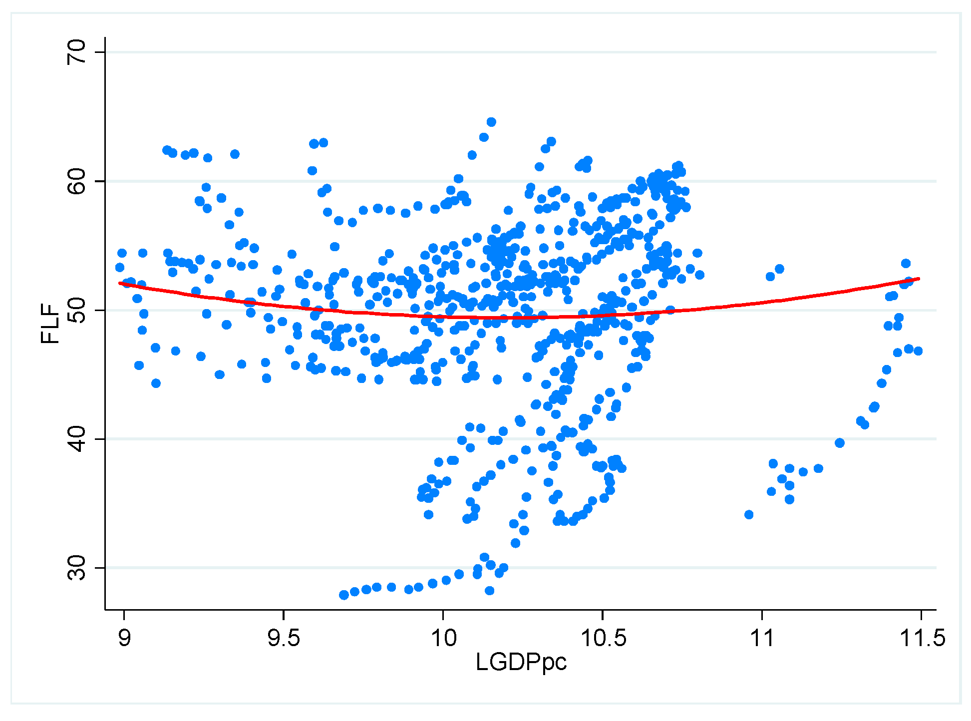
Before presenting our estimation results, it is worth first focusing on the visual representation of the data. In Figure 1, Figure 2 and Figure 3 we show the scatter plots of the association between FLFPit and GDPpcit for the EU-28, EU-15 and EU-13 countries, respectively.
Figure 1 confirms that the EU-28 countries follow a slight U pattern over the period 1990–2016. This is stable for individual survey time periods (not presented here). It was observed that both for relatively low and high levels of GDPpcit, FLFPit was around 50%, while for average per capita incomes, FLFPit was highly variable. In countries where lnGDPpcit ranged from approximately 9.5–10.5, women’s participation in the labour market was observed both at relatively high (over 60%) and low (below 30%) levels. Over the years under study, several countries have experienced significant increases in female labour force participation. However, despite positive changes, there are still economies lagging behind, not reaching the EU average FLFPit. Countries situated below the curve turning point are older member countries of the EU (except Denmark, Finland, Sweden and the UK) and some new member states (Malta, Cyprus, Bulgaria or Romania). However, most Eastern countries exhibited above average female labour participation rates. These economies of Eastern Europe represent cases of highly feminized labour forces because of the socialist commitment to and imperative for women’s economic mobilization [11].
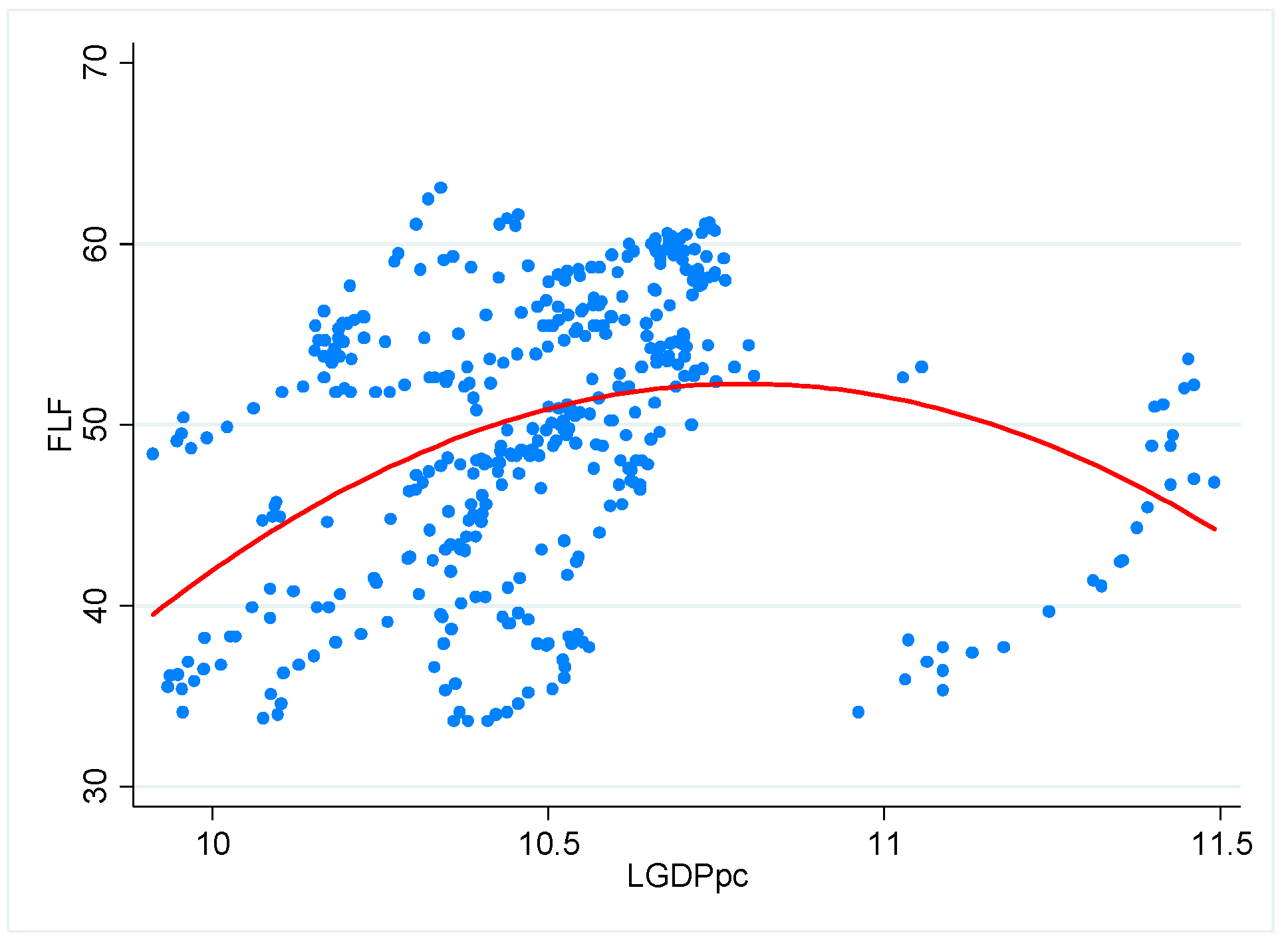
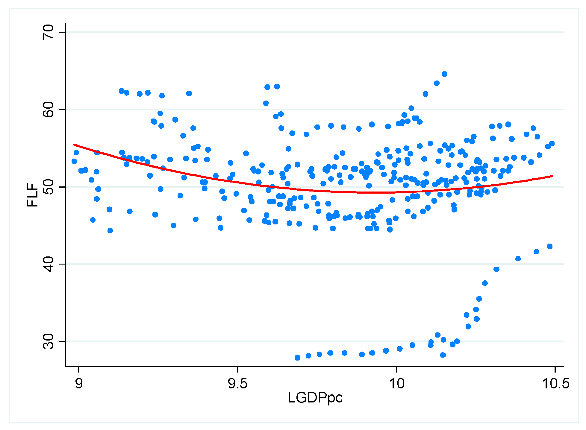
When we move to the distinction between the EU-15 countries (Figure 2) and the newest European countries (Figure 3), we find mixed results, indicating the relevance of contextual factors in determining the FLFPit-GDPpcit relationship. In the former group of countries, an inverted U-shape is found whereas in the latter one, a slight U-shape relationship is identified.
Given this, and in order to gain a better understanding of the relationship between FLFPit and GDPpcit, we report the estimation results for our sample.
We first present the results for the static models (OLS and FE) for all EU countries in Table 2. We report for each regression the coefficients for GDP per capita (in logs), GDP per capita squared (in logs), the control variables as well as the turning point (time-fixed effects are included). It shows that there was a statistically significant U relationship in both OLS and FE estimations when control variables were not included.
There was a variability in turning points between the estimations, being lower in the FE estimator than in the OLS one, similar to the findings in Gaddis and Klasen [15]. The turning point occurs at $34,417 per capita (in 2011 constant prices) in OLS estimation without control variables and at $22,608 per capita (in 2011 constant prices) in the FE estimation without control variables.
When we included control variables, the U-shaped relationship remained significant only in the fixed-effect estimation. We are aware that many studies have noted that female education and fertility rates are strongly inversely correlated, creating a collinearity problem in the equations. For this reason, we have run the models with and without the fertility rate variable, and results remain largely unchanged. The coefficients of education variables were positive and statistically significant meaning that an increase in the education level leads to higher female labour participation. The tertiary education had greater value than the secondary education. The unemployment rate held a negative and significant coefficient. Unemployment rates had a statistically negative effect. This is an indication of the existence of a discouraged worker effect, which occurs during recessions when workers do not search for work because they view their chances of finding a suitable job as being too low. This result was also found by Ozerker [29]. Finally, life expectancy and fertility rates were not statistically significant. In Appendix A, we present a robust test for the U-shaped relationship.
The static models for the entire group of EU countries suggest that, in general terms, the FLFP and economic development relationship followed a U-shaped pattern over the period analysed. The downward slope of the curve exhibited the de-feminization process of the labour force that is associated with economic development. Countries in the early stages of development are exposed to structural changes that encourage women in low-paid jobs to join the education system [14]. The upward slope suggests the empowerment process in women is growing due to further economic development.
Moving to the estimations of the two groups of EU countries included in the study (Table 3), we find that the U-shaped relationship between FLFP and GDPpc only holds for new member states. We observed that in both estimators (OLS and FE), the coefficient of GDPpc was much larger than the one of the squared GDPpc, which might suggest that the “negative” relationship between FLFP and GDPpc was dominant.
For the EU-15 group of countries, there was no evidence of a U relationship since the corresponding coefficients were not statistically significant (except in the OLS estimation without controls where an inverse U-shaped relationship was found).
For the two groups of countries, the coefficients for education variables were positive and statistically significant. The unemployment rate was statistically non-significant (except for UE-15 in OLS estimations with controls) although it had a negative sign, as do the estimations for the whole of Europe. The remaining variables were not statistically significant (except for the life expectancy in EU-13, which was significant and negative in OLS estimations with controls). In Appendix A, we present a robust test for the U-shape relationship.
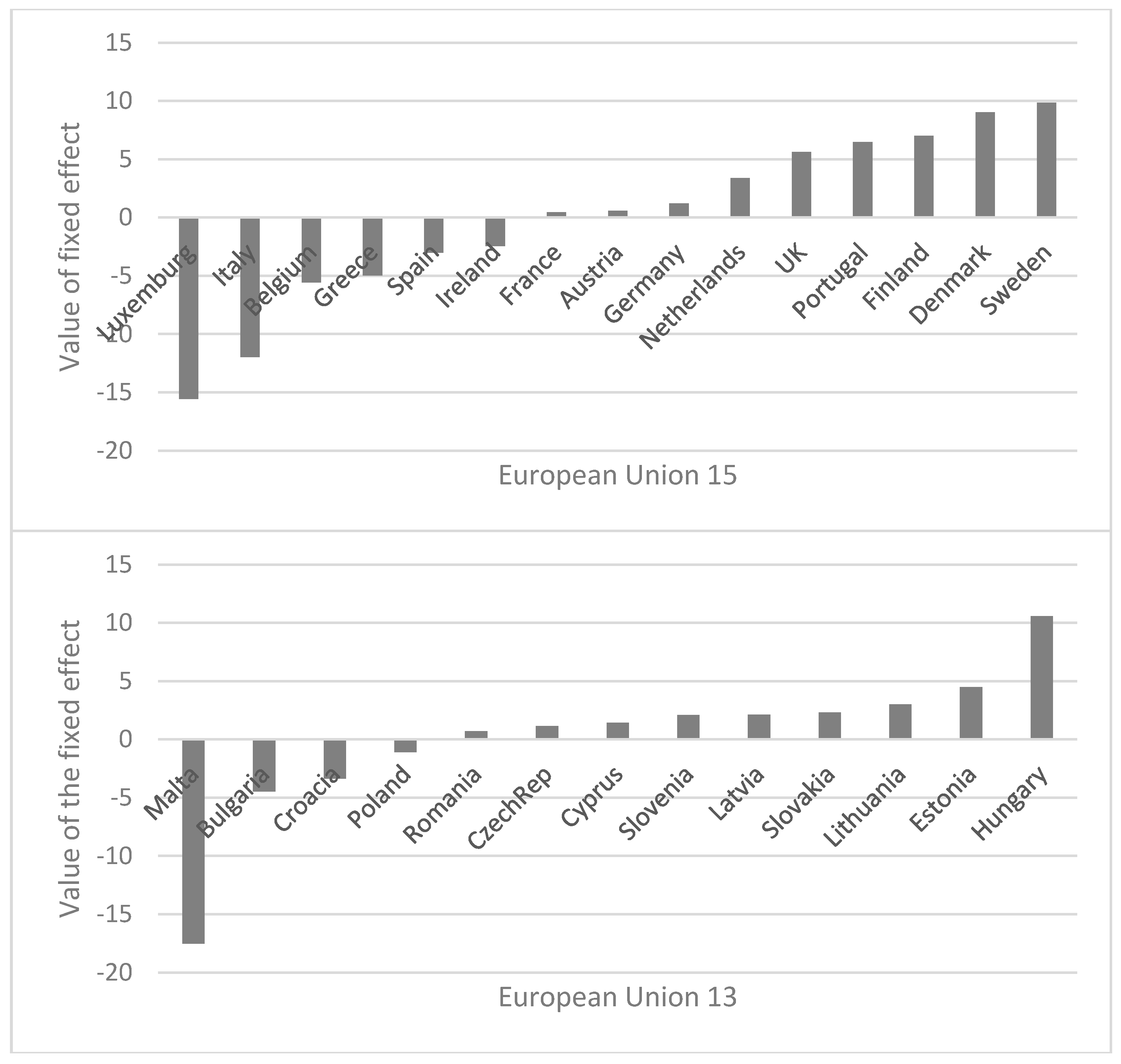
Besides the signs and significance levels of the GDP variables, the fixed-effect regressions also provide useful information on country-specific differences in FLFP, which cannot be explained by the level of GDP or over time changes. Figure 4 shows the estimated fixed effects using the regression without controls revealing the countries with the largest positive and negative fixed effects. The figures unveil striking regional patterns in female labour force participation, which are conditioned on the level of GDP.
Most Eastern transition countries (Hungary, Estonia, Slovenia, Lithuania, Czech Republic and Latvia) had large positive effects confirming the idea that the region has above average rates of FLFP because of the legacy of socialism, which promoted female labour force participation [15,47].
Figure 4 also shows the pattern of FLFP for EU-15 countries, with negative fixed effects in Southern European countries (Italy, Spain and Greece) along with other countries such as Luxemburg or Belgium. The largest positive fixed effects are associated with Northern countries (Finland, Denmark and Sweden). These results reveal, as stated by Gaddis and Klasen [15] the strong influence of the history of the countries in determining the evolution of the labour force participation.
The use of dynamic models (i.e., GMM) allows us to capture, at least partially, the influence of past values of FLFP, that is, the power of history. Table 4 displays the results of the difference of the GMM estimator for the EU-28 and the two subgroups of European countries. We report the turning points, sample sizes and regression diagnostics.
We observed the persistent behaviour of FLFP, as the coefficient of the first lag of the dependent variable was positive and highly significant in all cases. There are significant differences in the intensity of the persistence since in the EU-15 countries, the coefficient for this variable was 0.84 (significant at the 1% level) while in the EU-13 countries this coefficient was 0.24 and marginally statistically significant at the 10% level. This finding suggests that, for the latter group of European countries, past values of the FLFP do not contribute to forecasting future values of FLFP as much as in the EU-15 subgroup of countries. In other words, the resilience to recover from a shock was lower.
The FLFP and economic development relationship follows a U-shaped pattern when all European countries were considered. However, when the EU-28 was split into the two groups, we found that there was evidence for the feminization U hypothesis only in the newest European countries (EU-13). The coefficient, however, was only significant at the 10% level. We did not find such evidence for the old countries (EU-15), since the coefficients for GDP per capita (lnGDPpc) and the squared GDP per capita (lnGDPpc2) were statistically non-significant. The turning point for the former group of countries occurred at around $14,000 (at 2011 constant prices). Again, the negative relationship between female labour force engagement and level of per capita income was strong (lnGDPpc), compared to the positive one (lnGDPpc2). In the dynamic models, control variables were not statistically significant due to the high persistence of the female labour participation variable. In Appendix A, we present a robust test for the U-shape relationship.
5. Conclusions and Discussion
This paper studies the relationship between female labour force participation and economic development in the European Union countries over the period 1990–2016, distinguishing between the long-standing EU member countries (EU-15) and the new member states (EU-13) incorporated into the European Union in the extensions, which have taken place since 2004.
We have estimated static (OLS and fixed-effect estimators) and dynamic models (GMM estimator) with and without control variables. We control for life expectancy, fertility rate, secondary and tertiary education and unemployment rate. The most robust estimates, those based on GMM estimations with control variables, support the U-hypothesis for the EU-28, which suggests that in the early stages of economic development, female labour force engagement tends to fall, then as countries increase their development and become more serviced-based, the female labour force starts to grow.
Nevertheless, when the feminization hypothesis was tested in the two country clubs (old and new member states) separately, the results changed. For the EU-15 countries, the existence of the U-shaped relationship was not verified. Most of these countries were already high-income economies in the 90s, and female labour participation had almost reached its full potential. For the group of new member states, the U-shaped relationship was confirmed. However, the coefficients for this group of countries were only statistically significant at the 10% level, suggesting that evidence in favour of the feminization hypothesis is weak in this group of countries.
In all of the groups of countries, the results also show that female education had a positive effect on female labour force participation (although they were not statistically significant). Although the fertility rate had negative correlation with female labour force participation (in EU-13 countries), it was not statistically significant.
The differences between “old” and “new” member states regarding the relationship between FLFP and economic development suggest the desirability of achieving further progress in the deepening of the integration process as a solution to the possible dissimilarities in the level of resilience to cyclical and structural forces.
These findings regarding the relationship between female labour force participation and economic development in the European Union, however, should be interpreted with certain caution since the period analysed was not very long. Moreover, besides the traditional control variables considered in our analysis, there may be other factors affecting women’s labour participation such as legal and tax regulation, level of competition and liberalization or the openness of the country as claimed by Lechman and Kaur [14].
Thus, this work has extended the current empirical state of the art by providing additional evidence on the relationship between FLFP and economic development in the European context, which had not been examined to date.
Author Contributions
Conceptualization, A.G.-F. and C.G.-G.; Funding acquisition, A.A.; Investigation, A.A. and A.G.-F; Methodology, A.A. and C.G.-G.; Supervision, C.G.-G.; Writing—original draft, A.A. and A.G.-F.; Writing—review & editing, A.G.-F. and C.G.-G.
Funding
This research was funded by Eusko Jaurlaritza, grant number IT1052-16.
Acknowledgments
The authors acknowledge the financial support from the Research Group by the Basque Government “Institutions, Regulation and Economic Policy” (IT1052-16).
Conflicts of Interest
The authors declare no conflict of interest.
Appendix A
Given a model of the form
Lind and Mehlum (2010) [48] show that a test for the presence of U relationship needs to be based on the following joint null hypotheses:
H0:
against the alternative:
(α + 2βlnGDPpcmin ≤ 0) ∪ (α + 2βlnGDPpcmax ≥ 0), (1)
H1:
where, lnGDPpcmin and lnGDPpcmax are the minimum and maximum values of lnGDPpc, respectively. Lind and Mehlum [48] use Sasabuchi’s (1980) likelihood ratio approach to build a test for the joint hypothesis given by Equations (1) and (2). Table A1, Table A2, Table A3, Table A4 and Table A5 report the results of the Sasabuchi–Lind–Mehlum (SLM) test based on the results of Table 2, Table 3 and Table 4, respectively. (α + 2βlnGDPpcmin > 0) ∩ (α + 2βlnGDPpcmax < 0), (2)
The top panel of Table A1 shows that the marginal effect of lnGDPpc is negative and statistically significant at lnGDPpcmin and positive and statistically significant at lnGDPpcmax for models 1, 3 and 4. The bottom panel of the table shows that the SLM test rejects H0 (presence of inverse U-shape) for the aforementioned models and indicates that these results are consistent with the presence of a U relationship between lnGDPpc and FLFP.

Table A1.
Tests for a U-shape: EU-28.
| Test for Model 1 OLS | Test for Model 2 OLS with Controls | Test for Model 3 FE | Test for Model 4 FE with Controls | |
|---|---|---|---|---|
| Slope at GDPpc min | –50.65 ** | 49.77 ** | –215.27 *** | –120.31 *** |
| Slope at GDPpc max | 5.05 * | –5.50 ** | 31.67 *** | 17.75 *** |
| SLM test for inverse U shape | 1.25 | 1.72 (a) | 5.97 | 3.22 |
| p value | 0.10 | 0.04 | 0.00 | 0.00 |
| Fieller 90% confidence interval | (10.01; 52.82) | (5.75; 11.12) | (9.87; 10.21) | (9.73; 10.40) |
This table reports the results of the Sasabuchi–Lind–Mehlum test for a U-shaped relationship. Robust standard errors *** p < 0.01, ** p < 0.05, * p < 0.1. (a) Sasa- buchi-Lind-Mehlum (SLM) test for U-shape. The test rejects the H0 (presence of U-shape).
Table A2 shows results of the U-shape test for the EU-15 countries. Results for these regressions do not strongly support the presence of the U-shape. The marginal effect of lnGDPpc is positive and statistically significant at lnGDPpcmin (Model 5). The SLM tests rejects the null of existence of inverse U-shape against the alternative of U-shape or monotonic. For estimations 6–8, the marginal effect of lnGDPpc is negative but statistically non-significant at lnGDPpcmin.
Table A2.
Tests for a U-shape: EU-15.
| Test for Model 5 OLS | Test for Model 6 OLS with Controls | Test for Model 7 FE | Test for Model 8 FE with Controls | |
|---|---|---|---|---|
| Slope at GDPpc min | 275.35 *** | –44.39 | –88.18 | –34.59 |
| Slope at GDPpc max | –18.6024 *** | –5.93 | 18.43 *** | 12.73 ** |
| SLM test for U shape | 3.19 (a) | (b) | 1.19 | 0.54 |
| p value | 0.0012 | - | 0.118 | 0.296 |
| Fieller 90% confidence interval | (10.55–10.91) | (–Inf; +Inf) U (10.25; +Inf) | (–Inf; 14.67) U (10.30; +Inf) | (–Inf; 11.88) U (10.26; +Inf) |
This table reports the results of the Sasabuchi–Lind–Mehlum test for a U-shaped relationship. Robust standard errors *** p < 0.01, ** p < 0.05, * p < 0.1. (a) SLM test for inverse U-shape. The test rejects the null of existence of a U-shape. (b) Extremum outside interval—trivial failure to reject Ho (H0: monotone or U shape).
In Table A3, the top panel shows that the marginal effect of lnGDPpc is negative and statistically significant at lnGDPpcmin and positive and statistically significant at lnGDPpcmax for all models. The bottom panel shows that the SLM test rejects H0 (presence of U-shape) for model 9–11 suggesting that the results are consistent with the presence of a U relationship between lnGDPpc and FLFP.
Table A3.
Tests for a U-shape: EU-13.
| Test for Model 9 OLS | Test for Model 10 OLS with Controls | Test for Model 11 FE | Test for Model 12 FE with Controls | |
|---|---|---|---|---|
| Slope at GDPpc min | –111.51 | –153.75 ** | –256.14 *** | –136.96 ** |
| Slope at GDPpc max | 15.062 | 45.73 *** | 42.53 *** | 30.74 ** |
| SLM test for U shape | 0.71 | 1.72 | 3.43 | 1.78 |
| p value | 0.239 | 0.046 | 0.000 | 0.0412 |
| Fieller 90% confidence interval | (–Inf; +Inf) | (2.12; 9.38) | (9.64; 10.22) | (6.57; 10.43) |
This table reports the results of the Sasabuchi–Lind–Mehlum test for a U-shaped relationship. Robust standard errors *** p < 0.01, ** p < 0.05, * p < 0.1.
Table A4 shows that the marginal effect of lnGDPpc is negative and statistically significant at lnGDPpcmin and positive and statistically significant at lnGDPpc max, for both models. The SLM test rejects H0 (presence of U-shape) for models 13–14 suggesting that the results are in line with the feminization hypothesis.
Table A4.
Tests for a U-shape for dynamic panels: EU-28.
| Test for Model 13 GMM | Test for Model 14 GMM with Controls | |
|---|---|---|
| Slope at GDPpc min | –95.06 ** | –255.55 ** |
| Slope at GDPpc max | 27.98 *** | 62.07 *** |
| SLM test for U shape | 2.32 | 2.12 |
| p value | 0.0112 | 0.0182 |
| Fieller 90% confidence interval | (7.69; 9.37) | (8.15; 9.56) |
This table reports the results of the Sasabuchi–Lind–Mehlum test for a U-shaped relationship. Robust standard errors *** p < 0.01, ** p < 0.05, * p < 0.1.
Finally, Table A5 shows that the marginal effect of lnGDPpc is negative and statistically significant at lnGDPpcmin and positive and statistically significant at lnGDPpcmax for all models. The SLM test rejects H0 (presence of U-shape) suggesting that the results are consistent with the presence of the U relationship between lnGDPpc and FLFP for estimations 17–18. However, this hypothesis is not confirmed for estimations 15 and 16.
Table A5.
Tests for a U-shape for dynamic panels: EU-15 and EU-13.
| EU-15 | EU-13 | |||
|---|---|---|---|---|
| Test for Model 15 GMM | Test for Model 16 GMM with Controls | Test for Model 17 GMM | Test for Model 18 GMM with Controls | |
| Slope at GDPpc min | –101.52* | –125.32 * | –204.41 ** | –223.01 * |
| Slope at GDPpc max | 10.82** | 13.20 * | 42.14 ** | 44.26 * |
| SLM test for U shape | SLM test for U shape | SLM test for U shape | ||
| SLM test for U shape | 1.45 | 1.41 | 2.24 | 1.64 |
| p value | 0.0755 | 0.0814 | 0.0148 | 0.0538 |
| Fieller 90% confidence interval | (–Inf; 14.58) U (11.01; +Inf) | (–Inf; +Inf) | (8.95; 9.82) | (6.57; 10.43) |
This table reports the results of the Sasabuchi–Lind–Mehlum test for a U-shaped relationship. Robust standard errors *** p < 0.01, ** p < 0.05, * p < 0.1.
Figure A1.
Countries.

References
- International Monetary Fund. World Economic Outlook, Cyclical Upswing, Structural Changes. 2018. Available online: https://www.imf.org/en/Publications/WEO/Issues/2018/03/20/world-economic-outlook-april-2018 (accessed on 15 March 2019).
- Eurostat. Database on Economic and Finance. Available online: https://ec.europa.eu/eurostat/data/database (accessed on 14 March 2019).
- Montero, J.M.; Regil, A. The Cyclical Resilience and Determinants of the Participation Rate in Spain; Economic Bulletin; Bank of Spain: Madrid, Spain, 2015. [Google Scholar]
- Hijzen, A.; Kappeler, A.; Park, M.; Schwellnus, C. Labour Market Resilience: The Role of Structural and Macroeconomic Policies; Economics Department Working Papers 1406; OECD: Paris France, 2017; Available online: http://www.oecd.org/officialdocuments/publicdisplaydocumentpdf/?cote=ECO/WKP(2017) 38 (accessed on 15 March 2019).
- Sinha, J.N. Dynamics of female participation in economic activity. In Proceedings of the World Population Conference, Belgrade, Serbia, 30 Augus–10 September 1965; 4, pp. 336–337. [Google Scholar]
- Boserup, E. Women’s Role in Economic Development; St. Martin’s Press: New York, NY, USA, 1970. [Google Scholar]
- Durand, J. The Labour Force in Economic Development: A Comparison of International Census Data, 1946–1966; Princeton University Press: Princeton, NJ, USA, 1975. [Google Scholar]
- Pampel, F.C.; Tanaka, K. Economic development and female labor force participation: A reconsideration. Soc. Forces 1986, 64, 599–619. [Google Scholar] [CrossRef]
- Goldin, C. The U-Shaped Female Labor Force Function in Economic Development and Economic History; Working Paper No. 4707; National Bureau of Economic Research: Cambridge, MA, USA, 1994. [Google Scholar] [CrossRef]
- Goldin, C. The U-shaped female labor force function in economic development in economic history. In Investment in Women’s Human Capital; Schultz, T.P., Ed.; University of Chicago Press: Chicago, IL, USA, 1995. [Google Scholar]
- Çağatay, N.; Özler, Ş. Feminization of the labor force: The effects of long-term development and structural adjustment. World Dev. 1995, 23, 1883–1894. [Google Scholar] [CrossRef]
- Luci, A. Female labour market participation and economic growth. Int. J. Innovat. Sustain. Dev. 2009, 4, 97–108. [Google Scholar] [CrossRef]
- Tam, H. U-shaped female labor participation with economic development: Some panel data evidence. Econ. Lett. 2011, 110, 140–142. [Google Scholar] [CrossRef]
- Lechman, E.; Kaur, H. Economic growth and female labor force participation -verifying the U-feminization hypothesis. New evidence for 162 countries over the period 1990–2012. Econ Sociol. 2015, 8, 246–257. [Google Scholar] [CrossRef]
- Gaddis, I.; Klasen, S. Economic development, structural change, and women’s labor force participation. J. Popul. Econ. 2014, 27, 639–681. [Google Scholar] [CrossRef]
- Lahoti, R.; Swaminathan, H. Economic Development and Women´s Labor Force Participation in India. Fem. Econ. 2016, 22, 168–195. [Google Scholar] [CrossRef]
- Fatima, A.; Sultana, H. Tracing out the U-shape relationship between female labor force participation rate and economic development for Pakistan. Int. J. Soc. Econ. 2009, 36, 182–198. [Google Scholar] [CrossRef]
- Olivetti, C. The Female Labor Force and Long-Run Development: The American Experience in Comparative Perspective; Working Paper No. 19131; National Bureau of Economic Research: Cambridge, MA, USA, 2013. [Google Scholar] [CrossRef]
- Tansel, A. Economic Development and Female Labor Force Participation in Turkey: Time Series Evidence and Cross-Province Estimates; Working Papers in Economics; ERC—Economic Research Center, Middle East Technical University: Çankaya/Ankara, Turkey, 2002. [Google Scholar] [CrossRef]
- Tilly, L.A.; Scott, J.W. Women, Work and Family; Routledge: New York, NY, USA, 1987. [Google Scholar]
- Tsani, S.; Paroussos, L.; Fragiadakis, C.; Charalambidis, I.; Capros, P. Female labour force participation and economic growth in the South Mediterranean countries. Econ. Lett. 2013, 120, 323–328. [Google Scholar] [CrossRef]
- Verme, P. Economic Development and Female Labor Participation in the Middle East and North Africa: A Test of the U-Shape Hypothesis; The World Bank: Washington, DC, USA. [CrossRef]
- International Monetary Fund. 25 Years of Transition Post-Communist Europe and the IMF; Regional Economic Issues; Special Report; International Monetary Fund: Washington, DC, USA, 2014. [Google Scholar]
- International Monetary Fund. World Economic Outlook: Subdued Demand: Symptoms and Remedies; International Monetary Fund: Washington, DC, USA, October 2016. [Google Scholar]
- European Commission. Five Years of an Enlarged EU: Economic Achievements and Challenges; Office for Official Publications of the European Communities: Luxemburg, 2009. [Google Scholar]
- Psacharopoulos, G.; Tzannatos, Z. Female labor force participation: An international perspective. World Bank Res. Obser. 1989, 4, 187–201. [Google Scholar] [CrossRef]
- Schultz, T.P. International Differences in Labor Force Participation in Families and Firms, Economic Growth Center; Working Paper No. 634; Yale University: New Haven, CT, USA, 1991; Available online: http://hdl.handle.net/10419/160556 (accessed on 20 November 2018).
- Vlasblom, J.D.; Schippers, J.J. Increases in Female Labour Force Participation in Europe: Similarities and Differences. Eur. J. Popul. 2004, 20, 375–392. [Google Scholar] [CrossRef]
- Ozerkek, Y. Unemployment and labor force participation: A panel cointegration analysis for European countries. Appl. Econ. Int. Dev. 2013, 13, 67–76. [Google Scholar]
- Tasseven, O. The Relationship between Economic Development and Female Labor Force Participation Rate: A Panel Data Analysis; Hacioglu, Ü., Dincer, H., Eds.; Global Financial Crisis and its Ramification on Capital Market, Contributions to Economics; Springer: Berlin, Germany, 2017; pp. 555–568. [Google Scholar] [CrossRef]
- Goldin, C. The Quiet Revolution That Transformed Women’s Employment, Education, and Family. Am. Econ. Rev. 2006, 96, 1–21. [Google Scholar] [CrossRef]
- Akerlof, G.A.; Kranton, E. Economics and Identity. Q. J. Econ. 2000, 115, 715–753. [Google Scholar] [CrossRef]
- Mammen, K.; Paxson, C. Women’s work and economic development. J. Econ. Perspect. 2000, 14, 141–164. [Google Scholar] [CrossRef]
- Suh, M. Determinants of Female Labor Force Participation in South Korea: Tracing out the U-shaped Curve by economic growth. Soc. Indic. Res. 2016, 131, 255–269. [Google Scholar] [CrossRef]
- Mehrotra, S.; Parida, J.K. Why is the Labour Force Participation of Women declining in India? World Dev. 2017, 98, 360–380. [Google Scholar] [CrossRef]
- Dildar, Y. Patriarchal Norms, Religion, and Female Labor Supply: Evidence from Turkey. World Dev. 2015, 76, 40–61. [Google Scholar] [CrossRef]
- Heston, A.; Summers, R.; Aten, B. Penn Word Table Version 6.3. Center for International Comparisons of Production. Income and Prices; University of Pennsylvania: Philadelphia, PA, USA, 2009. [Google Scholar]
- Heston, A.; Summers, R.; Aten, B. Penn. Word Table Version 7.1. Center for International Comparisons of Production. Income and Prices; University of Pennsylvania: Philadelphia, PA, USA, 2012. [Google Scholar]
- Arellano, M.; Bover, O. Another Look at the Instrumental Variable Estimation of Error-Components Models. J. Econ. 1995, 68, 29–51. [Google Scholar] [CrossRef]
- Blundell, R.; Bond, S. Initial Conditions and Moment Restrictions in Dynamic Panel Data Models. J. Econ. 1998, 87, 115–143. [Google Scholar] [CrossRef]
- Bussmann, M. The effect of trade openness on women´s welfare and work life. World Dev. 2008, 37, 1027–1038. [Google Scholar] [CrossRef]
- Klasen, S.; Pieters, J. Push or Pull? Drivers of Female Labor Force Participation during India’s Economic Boom; Institute for the Study of Labor: Bonn, Germany, 2012; p. 6395. [Google Scholar]
- Cerrutti, M. Economic Reform, Structural Adjustment and Female Labor Force Participation in Buenos Aires, Argentina. World Dev. 2000, 28, 879–891. [Google Scholar] [CrossRef]
- Starr, M.A. Gender, added-worker effect, and the 2007–2009 recession: Looking within the household. Rev. Econ. Household 2014, 12, 209–235. [Google Scholar] [CrossRef]
- Mankart, J.; Oikonomon, R. The rise of the added work effect. Econ. Lett. 2016, 144, 48–51. [Google Scholar] [CrossRef]
- Gray, M.M.; Kittilson, M.C.; Sandholtz, W. Women and globalization: A study of 180 countries, 1975–2000. Int. Organ. 2006, 60, 293–333. [Google Scholar] [CrossRef]
- Kornai, J. The Socialist System. The Political Economy of Communism; Princeton University: Princeton, NJ, USA, 1992. [Google Scholar]
- Lind, J.T.; Mehlum, H. With or Without U? The Appropriate Test for a U-Shaped Relationship. Oxford B Econ. Stat. 2010, 72, 109–118. [Google Scholar] [CrossRef]
Figure 1.
Female labour force participation versus GDPpc. 28 EU countries. 1990–2016.

Figure 2.
Female Labour Force participation vs. GDPpc (EU-15 countries, 1990–2016).

Figure 3.
Female labour force participation versus GDPpc (EU-13 countries, 1990–2016).

Figure 4.
Country-specific fixed effects by country group. Fixed-effect regression based on the OLS without controls.
Figure 4.
Country-specific fixed effects by country group. Fixed-effect regression based on the OLS without controls.

Table 1.
Basic statistics of the whole sample, 1990–2016.
| Mean | SD | Min | Max | |
|---|---|---|---|---|
| FLFP | 50.0 | 7.2 | 27.9 | 64.6 |
| GDPpc | 30,236.6 | 14,379.0 | 8001.7 | 97,864.2 |
| Life expectancy | 80.0 | 2.9 | 72.6 | 86.3 |
| Fertility rate | 1.6 | 0.2 | 1.1 | 2.4 |
| Tertiary education | 22.3 | 9.4 | 3.9 | 43.2 |
| Secondary education | 43.8 | 13.0 | 11.6 | 70.4 |
| Female unemployment rate | 9.6 | 4.9 | 1.5 | 31.4 |
FLFP: Female Labour Force Participation; GDPpc: Gross Domestic Product per capita.
Table 2.
Static models (EU-28).
| Model 1 OLS | Model 2 OLS | Model 3 Fixed Effects | Model 4 Fixed Effects | |||||
|---|---|---|---|---|---|---|---|---|
| lnGDP_pc | –52.148 (30.49) | * | 51.258 (29.79) | –221.917 (26.39) | *** | –124.02 (29.78) | *** | |
| lnGDP_pc2 | 2.496 (1.49) | * | –2.477 (1.40) | 11.067 (1.36) | *** | 6.187 (1.52) | *** | |
| Life expectancy | –.450 (0.37) | –.258 (0.49) | ||||||
| Fertility rate | –1.548 (2.20) | –1.298 (2.27) | ||||||
| Secondary education | 0.154 (0.06) | *** | 0.212 (0.06) | *** | ||||
| Tertiary education | 0.455 (0.07) | *** | 0.353 (0.09) | **** | ||||
| Unemployment rate | –0.378 (0.11) | *** | –0.072 (0.08) | |||||
| Constant | 318.991 (318.99) | ** | –190.145 (114.23) | 1158.14 (128.16) | *** | 676.20 (148.56) | **** | |
| N | 163 | 148 | 163 | 148 | ||||
| F (7,155); F (12,135) F (7,128); F (12,108) | 1.71 | 13.37 | 20.70 | 16.30 | ||||
| Prob > chi2 | 0.090 | 0.000 | 0.000 | 0.000 | ||||
| Rho | 0.886 | 0.848 | ||||||
| N groups | 28 | 28 | ||||||
| R-sq | 0.074 | 0.499 | ||||||
| R-sq: within | 0.530 | 0.644 | ||||||
| R-sq: between | 0.006 | 0.294 | ||||||
| R-sq: overall | 0.024 | 0.339 | ||||||
| Turning point | 34,417.3 | 31,156.9 | 22,608.2 | 22,530.6 | ||||
Cluster standard errors (country-level) in brackets. Time dummies included, but not reported. *** p < 0.01; ** p < 0.05; * p < 0.1. lnGDPpc: Gross Domestic Product per capita (in logs); lnGDPpc2: Squared of Gross Domestic Product per capita (in logs): OLS: Ordinary Least Squares
Table 3.
Static models (EU-15 and EU-13).
| EU-15 | EU-13 | |||||||||||||||
|---|---|---|---|---|---|---|---|---|---|---|---|---|---|---|---|---|
| Model 5 OLS | Model 6 OLS | Model 7 Fixed Effects | Model 8 Fixed Effects | Model 9 OLS | Model 10 OLS | Model 11 Fixed Effects | Model 12 Fixed Effects | |||||||||
| lnGDPpc | 283.26 (105.26) | *** | –45.42 (99.82) | –91.04 (76.03) | –35.87 (66.20) | –114.92 (125.87) | –159.12 (92.34) | * | –264.18 (58.20) | *** | –141.46 (79.23) | * | ||||
| lnGDPpc2 | –13.17 (4.91) | *** | 1.72 (4.58) | 4.78 (3.58) | 2.12 (3.10) | 5.67 (6.40) | 8.94 (4.73) | * | 13.38 (3.05) | *** | 7.51 (4.13) | * | ||||
| Life expectancy | –1.01 (.63) | 0.71 (0.90) | –2.38 (0.51) | *** | –0.314 (0.83) | |||||||||||
| Fertility rate | –4.68 (3.19) | 3.26 (4.51) | –6.97 (4.25) | –4.17 (3.75) | ||||||||||||
| Secondary education | 0.13 (0.06) | ** | 0.19 (0.07) | ** | 0.24 (0.051) | *** | 0.30 (0.15) | * | ||||||||
| Tertiary education | 0.59 (0.11) | *** | 0.31 (0.12) | ** | 0.39 (0.061) | *** | 0.48 (0.19) | *** | ||||||||
| Unemployment rate | –0.63 (0.14) | *** | 0.03 (0.10) | –0.08 (0.17) | 0.04 (0.21) | |||||||||||
| Constant | –1473.61 (562.31) | ** | 410.86 (522.84) | 475.93 (403.66) | 116.24 (363.50) | 631.14 (615.82) | 929.39 (459.28) | ** | 1353.04 (278.06) | *** | 0.722.76 (407.84) | * | ||||
| N | 90 | 86 | 90 | 86 | 73 | 62 | 73 | 62 | ||||||||
| F(7,82); F(12,73) F(7,68) F(12,59) F(7,65) F(11,50); F(7,53) F(11,38) | 3.37 | 17.31 | 17.91 | 15.53 | 0.61 | 10.07 | 5.47 | 2.79 | ||||||||
| Prob > chi2 | 0.003 | 0.000 | 0.000 | 0.000 | 0.7479 | 0.000 | 0.000 | 0.009 | ||||||||
| Rho | 0.896 | 0.906 | 0.845 | 0.709 | ||||||||||||
| N groups | 15 | 15 | 13 | 13 | ||||||||||||
| R-sq | 0.223 | 0.638 | 0.06 | 0.689 | ||||||||||||
| R-sq: within | 0.648 | 0.7595 | 0.419 | 0.446 | ||||||||||||
| R-sq: between | 0.002 | 0.1335 | 0.017 | 0.509 | ||||||||||||
| R-sq: overall | 0.068 | 0.2376 | 0.042 | 0.523 | ||||||||||||
| Turning point | 46,663.7 | 542,253.2 | 13,732.50 | 4703.90 | 25,185.90 | 7327.1 | 19,298.3 | 12,239.7 | ||||||||
Cluster standard errors (country-level) in brackets. Time dummies included, but not reported. *** p < 0.01; ** p < 0.05; * p < 0.
Table 4.
Dynamic models: GMM estimator (EU-28, EU-15 and EU-13).
| EU-28 | EU-15 | EU-13 | ||||||||||
|---|---|---|---|---|---|---|---|---|---|---|---|---|
| Model 13 | Model 14 | Model 15 | Model 16 | Model 17 | Model 18 | |||||||
| Female Labour Force Participation (t − 1) | 0.77 (0.14) | *** | 0.70 (0.19) | *** | 0.76 (0.08) | *** | 0.84 (0.13) | *** | 0.61 (0.22) | *** | 0.24 (0.13) | * |
| lnGDPpc | –98.38 (42.39) | ** | –264.10 (124.50) | *** | –104.54 (71.80) | –129.05 (82.78) | –211.04 (94.35) | ** | –230.19 (140.39) | * | ||
| lnGDPpc2 | 5.51 (2.25) | ** | 14.23 (6.48) | ** | 5.03 (3.31) | 6.21 (3.95) | 11.049 (4.86) | ** | 11.98 (7.26) | * | ||
| Life expectancy | 0.92 (0.97) | 0.45 (0.35) | 0.415 (0.66) | |||||||||
| Fertility rate | 19.13 (15.62) | 1.72 (2.48) | –0.545 (3.77) | |||||||||
| Secondary education | 0.12 (12.56) | 0.01 (0.06) | 0.203 (0.15) | |||||||||
| Tertiary education | –0.06 (15.25) | –0.04 (0.12) | 0.162 (0.17) | |||||||||
| Unemployment rate | 0.07 (0.24) | –0.06 (0.05) | –0.057 (0.13) | |||||||||
| N | 112 | 119 | 60 | 60 | 52 | 49 | ||||||
| Wald Chi2(9)(14)(9)(14)(9)(14) | 153.0 | 307.4 | 469.8 | 5167.7 | 57.43 | 1330.48 | ||||||
| Prob > chi2 | 0.000 | 0.0000 | 0.000 | 0.000 | 0.000 | 0.000 | ||||||
| N groups | 28 | 28 | 15 | 15 | 13 | 13 | ||||||
| Number of instruments | 13 | 18 | 13 | 14 | 10 | 11 | ||||||
| 2nd order autocorrelation | 0.610 | 0.675 | 0.105 | 0.174 | 0.510 | 0.324 | ||||||
| Hansen test of over identifying. restrictions | 0.177 | 0.136 | 0.408 | 0.335 | 0.244 | 0.313 | ||||||
| Turning point | 7472.9 | 10,682.9 | 32,328.1 | 32,660.7 | 14,047.3 | 14,899.4 | ||||||
Standard errors in brackets. Time dummies included, but not reported. *** p < 0.01; ** p < 0.05; * p < 0.1.
© 2019 by the authors. Licensee MDPI, Basel, Switzerland. This article is an open access article distributed under the terms and conditions of the Creative Commons Attribution (CC BY) license (http://creativecommons.org/licenses/by/4.0/).
Share and Cite
MDPI and ACS Style
Altuzarra, A.; Gálvez-Gálvez, C.; González-Flores, A. Economic Development and Female Labour Force Participation: The Case of European Union Countries. Sustainability 2019, 11, 1962. https://0-doi-org.brum.beds.ac.uk/10.3390/su11071962
AMA Style
Altuzarra A, Gálvez-Gálvez C, González-Flores A. Economic Development and Female Labour Force Participation: The Case of European Union Countries. Sustainability. 2019; 11(7):1962. https://0-doi-org.brum.beds.ac.uk/10.3390/su11071962
Chicago/Turabian StyleAltuzarra, Amaia, Catalina Gálvez-Gálvez, and Ana González-Flores. 2019. "Economic Development and Female Labour Force Participation: The Case of European Union Countries" Sustainability 11, no. 7: 1962. https://0-doi-org.brum.beds.ac.uk/10.3390/su11071962
Note that from the first issue of 2016, this journal uses article numbers instead of page numbers. See further details here.