Impact of Population Density on PM2.5 Concentrations: A Case Study in Shanghai, China


The Center for Modern Chinese City Studies, Future City Lab ECNU, School of Urban and Regional Science, East China Normal University, Shanghai 200241, China
*
Author to whom correspondence should be addressed.
Sustainability 2019, 11(7), 1968; https://0-doi-org.brum.beds.ac.uk/10.3390/su11071968
Submission received: 11 March 2019
/
Revised: 27 March 2019
/
Accepted: 29 March 2019
/
Published: 2 April 2019
Abstract
:We examine the effects of the urban built environment on PM2.5 (fine particulate matter with diameters equal or smaller than 2.5 μm) concentrations by using an improved region-wide database, a spatial econometric model, and five built environment attributes: Density, design, diversity, distance to transit, and destination accessibility (the 5Ds). Our study uses Shanghai as a relevant case study and focuses on the role of density at the jiedao scale, the smallest administrative unit in China. The results suggest that population density is positively associated with PM2.5 concentrations, pointing to pollution centralization and congestion effects dominating the mitigating effects of mode-shifting associated with density. Other built environment variables, such as the proportion of road intersections, degree of mixed land use, and density of bus stops, are all positively associated with PM2.5 concentrations while distance to nearest primary or sub-center is negatively associated. Regional heterogeneity shows that suburban jiedao have lower PM2.5 concentrations when a subway station is present.
1. Introduction
With rapid urbanization, many cities in China are suffering from one of the worst levels of air pollution in the world [1,2,3]. In 2015, there were 86 days during which average air pollution levels exceeded the standards set in China for PM2.5 (fine particulate matter with diameters equal or smaller than 2.5 μm), O3, and PM10 (fine particulate matter with diameters equal or smaller than 10 μm), the principal air pollutants. Of those, PM2.5, the main pollutant in China [4,5], accounted for 66.8% of the days when pollution levels were too high, and O3 and PM10 accounted for 16.9% and 15% each, respectively. There is growing evidence that long-term exposure to PM2.5 contributes to increased risk of cardiovascular disease [6,7] and mortality [8,9,10]. A 2013 meta-analysis of studies worldwide indicates that a 10 μg/m3 incremental increase in long-term average ambient PM2.5 concentrations is associated with approximately a 6% increased risk of all-cause mortality and a 15% increased risk of cardiovascular disease mortality [8]. Increases of PM2.5 concentrations also reduces the happiness of urban residents [11,12]. On polluted days, people are more likely to engage in impulsive and risky behavior that they may later regret [13]. Such behavior may be rooted in short-term depression and anxiety. Therefore, reducing PM2.5 is the key task for air quality improvement. Of the two mains sources of local emissions of PM2.5, industrial production and transportation [14], the present research focuses on transportation. Transportation is closely related to the urban built environment through traffic infrastructure and the travel behaviors of residents [14,15].
The effect of density on air pollution remains the subject of controversy despite the significant evidence urban geographers and urban planners have gathered on the relationships between the urban built environment and air pollution. High density areas are more likely to be non-motorized due to proximity, thereby reducing traffic-related emissions [16,17]. Another view holds that excessive population centralization will lead to traffic congestion and centralization of pollutants, resulting in increased pollution concentrations [18,19]. The main differences between these two vies may lie in the different types of data used (disaggregate and aggregate data) and the differences in the study areas. It is not clear, then, whether a high density urban built environment decreases traffic emissions.
This paper, taking Shanghai as a case study, examines the impact of the urban built environment, especially density, on PM2.5 concentrations. We attribute this finding to the dominant role of centralization and congestion effects over mode shifting effects. Given the persistent gaps in the literature, including the neglect of spatial dependency, low data resolution, and the omission of built environment attributes, this study contributes to the literature with more robust evidence. We use an improved region-wide PM2.5 database, apply a spatial econometric model for estimation, and consider five built environment attributes, density, design, diversity, distance to transit, and destination accessibility (5Ds), in the model to capture the comprehensive effect of the built environment.
2. Literature Review and Theoretical Hypothesis
Much literature has explored the influence of the urban built environment on air pollution. The urban built environment, which shapes transport behaviors, is typically classified into five elements: (1) Density, (2) design, (3) diversity, (4) distance to transit, and (5) destination accessibility [20,21]. PM2.5 concentrations, air pollution, emissions, density, population density, and built environment were used as keywords to search the literature; in particular, much attention was paid to the impact of density on PM2.5 concentrations.
2.1. Density
The large amount of literature on the relationship between density and air pollution can be split into disaggregate and aggregate studies according to the sample data types. Disaggregate data is based on individual-level surveys and calculates individual emissions from reported travel information. Aggregate data refers to actual measured regional air pollution data, mainly from satellite remote sensing and ground observation stations. Studies that rely on disaggregated data tend to show a negative link between population density and individual motor vehicle emissions. Under the assumptions these studies work under, areas with high population density will have shorter travel distances between housing and employment and switch individuals’ travel mode from private vehicles to public transit or walking, so as to reduce individual traffic off-gas emissions [22,23,24,25,26]. Gaigné et al. (2012), however, based on a theoretical model, stated that policies aimed at increasing density affect wages, prices, and land rent, which in turn incentivizes households and firms to reselect locations and generate higher levels of pollution [27].
Most studies based on aggregate data, on the other hand, suggest that higher urban population density will not only concentrate private car use, but also cause congestion and slower travel speeds, and therefore increase pollutant concentrations [18,19,28,29]. However, studies at lower levels of aggregation found a negative link between density and traffic emissions. New urbanism and smart growth have advocated a more compact, diversified, and walkable built environment by delineating urban growth boundaries and infilling development to alleviate traffic emissions caused by high dependencies on cars [30,31,32]. Many new urbanists argue that high density reduces traffic emissions by improving accessibility and reducing car-use [16,17], and that further, a smart growth mode focusing on urban redevelopment is also conducive to the slowing down of urban sprawl, which leads to a decrease in commuting distances and the protection of suburban ecology [33].
Although, from the view of aggregate data, new urbanism and smart growth have guided the planning and construction of some American cities, controversies on their applicability have been raised in China. Different from the low-density sprawl in American cities, residences and employment in Chinese cities are still localized in the center of the city, where it is still densely populated and has not experienced shrinking [34]. In short, due to these differences in cities, whether Chinese cities, especially mega-cities, are suitable for the high-density mode planning requires more empirical testing.
2.2. Design
Design in the context of the relationship between the built environment and air pollution is largely confined to measures of road and road intersection density. Research on these relationships showed that improvements to road network connectivity can alleviate congestion to some extent [35]. However, studies that attempted to analyze this link more rigorously found that a high density of intersections causes more speed changes and a lower average travel speed, which all together reduce fuel efficiency and increase exhaust emissions [15,36,37,38].
2.3. Diversity
A more diverse mix of land uses is beneficial to achieving an employment-housing balance. It contributes to shortening travel lengths, thus reducing car driving [39,40], and, consequently, decreasing traffic-related emissions. However, a greater availability of service facilities will increase residents’ travel frequency and augment traffic emissions in densely populated cities [41]. Yang and Cao (2018) found that the higher the community land use mixture, the more likely it will be for residents to emit more exhaust during recreational activities [42].
2.4. Distance to Transit
A convention in the mainstream literature is that the shorter the distance to bus stops, the more likely travelers are to employ public modes of transportation [43,44,45]. This reduces exhaust emissions since transit trips have lower per-person emissions than car driving [46]. However, recent studies demonstrate that living near bus stops does not significantly change the travel mode of existing car drivers [47,48,49], and a single bus, using diesel rather than gasoline, emits more pollutants compared with a private car because of a lower fuel efficiency. Moreover, buses have a higher frequency of stops/starts than private cars, which further increases emissions [50]. Another hotspot of public transit research is rail transit. Based on the same general argument as with bus stops, highly accessible stations lead residents to switch to rail transit and reduce local emissions in the process [51,52,53]. However, in this case too, some studies have found that this mode-shifting effect does not exist, especially for cars [54].
2.5. Destination Accessibility
Kahn (2000), in a study based in the United States, declared that residents of suburbs, often low to very low density areas, tend to rely on private cars for their commute, which are also longer [55]. It follows that more traffic emissions should be expected in suburbs than in city centers [56]. However, these results are context specific. China is characterized by different built environment attributes. Generally, the further residents are from the city center, the lower the likelihood of private car ownership and the lower the emissions [57,58].
2.6. Theoretical Hypothesis
Based on the overview of the literature, it is apparent that the effects of the built environment, especially population density, on air pollution are mixed. It does not mean that some conclusions are correct and others are wrong. As we have discussed, the conclusions may vary with the context and data types. Therefore, to minimize these issues, we propose a theoretical hypothesis about the relationship between population density and pollutant emissions.
High density has the following three effects: (1) Mode-shifting effect: High population density shortens individual trip distances between houses and places of employment and enables walking and biking, thus reducing private car dependency and decreasing traffic emissions; (2) congestion effect: An increase in the population density above a certain threshold will lead to high traffic congestion, lower driving speeds, and increased frequency of speed changes, all of which will reduce energy efficiency and increase exhaust emissions; (3) pollution centralization effect: Even if individual emissions decrease in dense areas, a high population density drives up the total number of driving cars, leading to an increase in total vehicle trips. If the mode-shifting effect is larger than the total of the congestion and centralization effects, a high density may be related to emissions reduction; otherwise, high density will result in a higher exhaust emission intensity. Therefore, the final effect of density on pollutant emission intensity depends on the relative magnitude of the three effects.
In addition, we identified three shortcomings in the previous literature, which might lead to ambiguous evidence and contribute to the mixed findings. First, due to the airborne nature of pollutants, pollution in adjacent areas influences each other. That is, there is a strong spatial autocorrelation of air pollutants in adjacent areas. However, most previous studies lack consideration of this factor and use classical statistical methods, such as ordinary least squares (OLS) [18,19] and correlation coefficients [59], which assume independent distribution, leading to estimation bias. Second, the resolution at which pollutant data are mapped in aggregate studies is usually 10 km × 10 km [60,61], which is too imprecise to identify the effect of the built environment at the scale of a city. City boundaries are irregular, so that too low a resolution can lead to erroneous descriptions of the values within city boundary areas. Third, the five types of built environment attributes are closely related and cumulatively describe the different aspects of the built environment. No studies have yet focused on all five attributes, which may cause omitted variables estimation bias. This study aims to address these shortcomings with more precise data and a robust method.
3. Methodology and Data
3.1. Research Framework
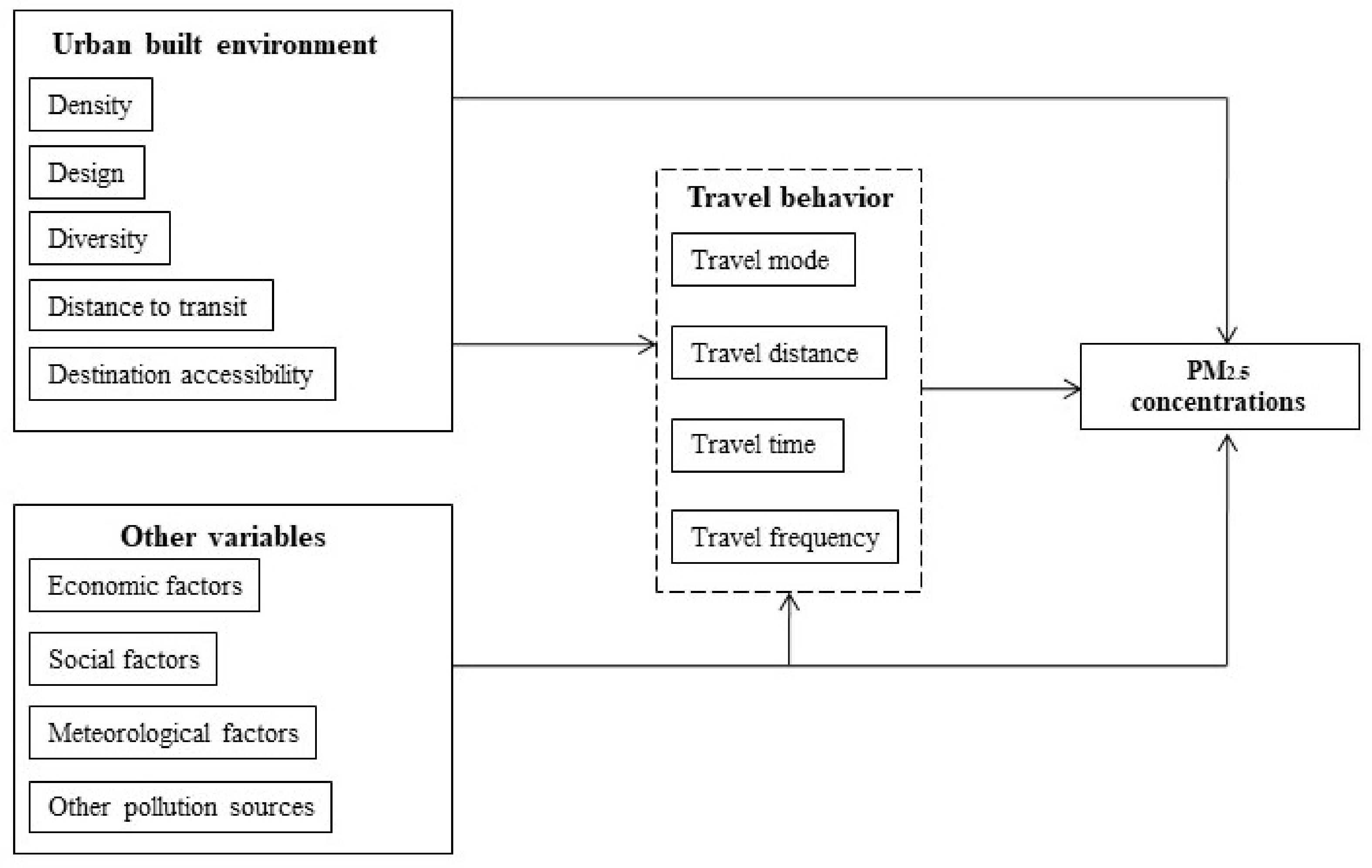
The objective of this paper is to examine the impact of the urban built environment on PM2.5 concentrations with a focus on density. We begin with the following theoretical framework (shown in Figure 1). The urban built environment attributes, often shortened to the ‘5Ds,’ are density, design, diversity, distance to transit, and destination accessibility [20]. Together, these attributes affect PM2.5 concentrations through residents’ travel behaviors, including travel mode, travel distance, travel time, and travel frequency. Constrained by data availability, these behavior variables are not directly measured and included in our model. Still, they are indispensable as mediating variables and are therefore marked with the dashed box. PM2.5 concentrations depend only on emissions and diffusion conditions, which is directly determined by the built environment, economic, social, meteorological, and other pollution related factors, which we can more easily include. For the selection of specific variables, emission factors mainly include road, bus stop density, subway station density, and pollution enterprises. Diffusion factors mainly include density, monsoon (represented by distance from the southeast point), etc. This comprehensive framework reduces the risk of omitting variables that influence PM2.5 concentrations, thus reducing bias in our estimation.
The jiedao (in Chinese, a grassroots administrative division in China) was selected as a spatial alternative. There are several reasons: Firstly, previous studies have regarded the city as a homogeneous surface. However, the actual population distribution within the city is highly uneven. The population density will rapidly decay or increase at distances from a few kilometers to a dozen kilometers. Therefore, it is necessary to explore the impact of density changes within the city. Secondly, the jiedao (or town) is the smallest administrative unit in China. The average area of a Shanghai jiedao is as small as 30 km2, which can finely capture the spatial differences of population density and PM2.5 concentrations inside the city. Finally, this paper takes travel behavior as a mediator between density and PM2.5 concentrations. Likewise, scholars who study travel behavior are paying increasingly more attention to microscopic geographic units, such as the traffic analysis zone [62,63] and Chinese jiedao [64].
3.2. Model
Previous studies have used multifarious research strategies to estimate the influence of built environment attributes on air pollution [29,65,66,67]. Given that administrative divisions do not constrain the diffusion of PM2.5, we expect significant spatial dependency between adjacent regions, which violates the independent distribution assumption of the error term in OLS estimation. Therefore, we chose a spatial econometric model specification for the regressions. The spatial econometric model fully considers the spatial dependence among the cross-sectional units, and builds a spatial weight matrix to incorporate the positional relationship among units. The matrix of weights can be based on whether spatial units are adjacent, a straight-line distance, or transport distance. Spatial econometric models are further differentiated between a spatial error model (SEM) and spatial lag model (SLM). When the spatial dependence of the interpreted variables has a significant effect on the model, the SLM is more appropriate. When the model error terms are spatially related, an SEM is used. Regardless of their respective strengths, the SEM and SLM are appropriate whenever variables are spatially correlated, but it is necessary to test for spatial effects of the dependent variable to choose one or the other. The results of the relevant tests are shown in Table 1.
First, the Moran’s I is positive and significant at the 1% level. It indicates that regions with high PM2.5 concentrations are generally surrounded by similar regions, and vice versa. This phenomenon supports the existence of spatial dependency among adjacent regions and complies with the conditions for spatial econometric estimations. Second, for both the Lagrange multiplier (LM) and robust Lagrange multiplier (robust LM), which indicate whether the model’s error term has a sequence correlation, the significance of the SLM is superior to the SEM. According to Anselin (2013), when the significance of the SLM is superior to the SEM, and the SLM is significant and the SEM is not, the SLM should be chosen [68]. We conclude that the SLM is the optimal method for this study and thus applied the following Formula:
where Yi and Yj refer to PM2.5 concentration values of jiedao i and j; Xir is the independent variable, r, in jiedao i, m represents the number of independent variables, and n = 225, which represents the number of jiedao in Shanghai; Wij is a matrix of spatial weights indicating the spatial relationship between jiedao i and j. We set an inverse distance weight matrix (1/dij), which means that the smaller the distance between jiedao, the bigger the weight.
Yi = ρWijYj + ∑βrXir + ε, ε~N (0, δ2)
The vector of independent variables includes measures of the five urban built environment attributes and other control variables. In this paper, the urban built environment variables were the population density, proportion of road intersections, degree of mixed land use, distance to nearest primary or sub-center, and density of bus stops. Other control variables included the economic density, gender ratio, influence of adjacent regions, density of pollution intensive firms, and meteorological factors [56,69,70].
3.3. Measurement of Variables and Data
In May 2012, the China National Environmental Monitoring Centre issued the “PM2.5 automatic testing instrument specifications and requirements”, which require all major cities to monitor PM2.5 concentrations. In 2013, the first full year of environmental air quality monitoring and implementation, the number of high air pollution days (air quality index > 100) in Shanghai was 125. PM2.5, as the primary and most common pollutant, was responsible for the index being above the threshold on 70.2% of those days. Therefore, we focused specifically on the impact of urban built environment characteristics on PM2.5 concentrations for 2013. The Shanghai government consists of 15 municipal districts and one county through which it collects data on 225 jiedao as local indicators for the towns, industrial parks, etc. The correspondence between jiedao and local areas allows us to match data from different sources. Herein, we refer to those areas of data gathering simply as jiedao.
The Socioeconomic Data and Applications Center (SEDAC) established at Columbia University in the United States aims to provide information pertinent to scientific and social-economic studies all over the world. The Center has assembled a database that includes 1998 to 2016 global surface PM2.5 concentrations in raster format at the 1 km × 1 km definition. It estimates ground-level fine particulate matter (PM2.5) by combining aerosol optical depth (AOD) retrievals from the National Aeronautics and Space Administration (NASA), Moderate Resolution Imaging Spectroradiometer (MODIS), Multiangle Imaging spectroradiometer (MISR), and Sea wide field remote sensor (SeaWIFS) instruments with the global 3-D model of atmospheric chemistry driven by meteorological input from the Goddard Earth Observing System (GEOS-Chem) chemical transport model, and subsequently calibrated to global ground-based observations of PM2.5 using geographically weighted regression (GWR) [71].
The combination of the SEDAC data with the Shanghai-specific data enables us to greatly improve on the PM2.5 resolution used in many previous studies. We used the Shanghai jiedao-scale administrative zoning map to extract the raster data values from SEDAC with Arcgis software, and calculated PM2.5 concentrations values according to the following Formula:
where PM2.5i refers to the PM2.5 concentration value (μg/m³) in jiedao i; Sij is the area of the raster cell, j, in jiedao i; PM2.5ij is the PM2.5 concentration value of raster j in jiedao i; n represents the number of raster cells in jiedao i.
PM2.5i = (∑Sij × M2.5ij)/n
The urban built environment variables were defined as follows. Population density was calculated by using the permanent population of Shanghai jiedao from the Sixth National Census in 2010 divided by the corresponding jiedao area. Since serious collinearity issues exist between the density and density of road intersections (Pearson correlation coefficient = 0.7), the design variable was represented by the proportion of the total road intersections in Shanghai within the jiedao area. The types of roads included urban expressway, highways, county roads, and township village roads. We defined land use diversity as:
where MIXi is the degree of mixed land use of jiedao i; piq represents the area of type q in jiedao i; q = 1,…, n; n = 15. We used the Euclidean distance to calculate the distance to the nearest primary or sub-center. Shanghai has one primary urban center (People square) and four sub-centers (Xujiahui Jiedao, Wujiaochang Jiedao, Huamu Jiedao, Zhenru Jiedao), which was sourced from http://finance.ifeng.com/news/region/20110915/4591923.shtml. The density of bus stops was calculated by dividing the number of bus stops by the corresponding jiedao area. The bus stop data was sourced from the Beijing City Lab.
MIXi = −(∑piq × lnpiq)/ln(n)
To match the existing literature, we developed a number of control variables. Economic density, as measured by Gross Domestic Product (GDP) data at the jiedao scale, is difficult to obtain. As an alternative, we obtained the number of firms within the boundaries of each jiedao and normalized it to the jiedao area. Data on the number of firms was sourced from the Shanghai Economic Census in 2013 (http://www.stats.gov.cn/tjsj/pcsj/jjpc/3jp/indexch.htm).
The gender ratio is more easily measured. We included this measure because previous studies have suggested that males prefer to drive [72], so the gender ratio (male/female) can reflect the influence of social factors on PM2.5 concentrations through travel type. Data was sourced from the Sixth Census Data of Shanghai Jiedao in 2010 (http://www.stats.gov.cn/tjsj/tjgb/rkpcgb/dfrkpcgb/201202/t20120228_30403.html).
The volatile nature of air-borne pollutants creates issues of regional spillover. The 2013 Shanghai environment bulletin revealed that adjacent provinces significantly affect PM2.5 concentrations in Shanghai. Specifically, the region north-west of Shanghai had a particularly high level of spillover into the area while the influence of the region to the south-east remained relatively low [73]. Therefore, we selected a point (121.96° E, 30.79° N) at the southeastern corner of Shanghai, and treated the distance of each jiedao’s geometric center to this point as a proxy variable of the influence of adjacent regions. The further the distance is, the bigger the impact will be.
The density of pollution-intensive firms is another important contributor to local concentrations of pollutants. The Ministry of Environmental Protection of China published guidelines in 2010 that led to the selection of 15 kinds of industries as heavy pollution industries. We used this guideline to calculate the number of heavy pollution firms within jiedao to isolate the effect of industrial production. Heavy pollution industries included thermal power, steel, cement, electrolytic aluminum, coal, metallurgical, chemical, petrochemical, building materials, paper making, brewing, pharmaceutical, fermentation, textile, leather, and mining industries. Pollution intensive firms’ data was sourced from the Chinese Industrial Firms Database of 2013.
Finally, meteorological factors influence pollution levels. The temperature, precipitation, wind speed, etc., can all affect PM2.5 concentrations in a region. Given the difficulty of obtaining meteorological data precise enough to match Shanghai’s 225 jiedao, and the meteorological continuity between individual jiedao, differences between jiedao can be neglected. We therefore assumed that these factors are constant throughout the region and omitted them in this paper. Concerning all the variables, considering the unit and magnitude differences, and making the data structure smoother, PM2.5 concentrations, POPDEN, PROCROSS, DISTOWN, ECONDEN, and INFADJA, are logarithmically processed in Table 2. Correlations and variance inflation factor (VIF) of OLS were further calculated and showed that all VIF values were less than 4, indicating that the collinearity problem was not serious.
4. Empirical Results and Discussions
4.1. Descriptive Analysis
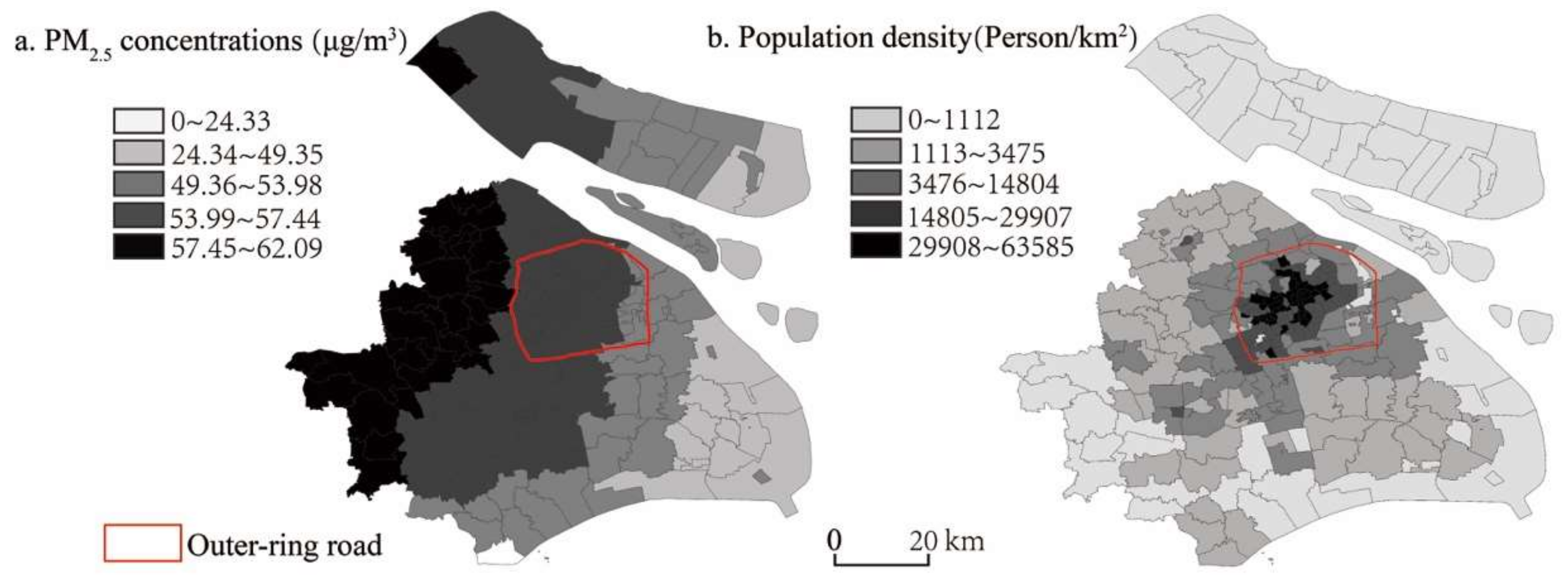
Figure 2 displays the spatial distribution of Shanghai’s PM2.5 concentrations and population density, in which the color scale is divided into five levels by the technique of “Jacks natural break point” in Arcgis, which can achieve the smallest variance within the group and the largest variance between groups. The concentrations of PM2.5 in Shanghai show a pattern of high concentrations in the northwest to low in the southeast, which confirms the important influence of adjacent areas. The World Health Organization (WHO) recommends average PM2.5 concentration values below 10 ug/m3 as the safe standard. People are vulnerable to diseases when concentrations reach 35 ug/m3. The mean PM2.5 concentrations in Shanghai is 55 ug/m3. There is therefore a great disparity with the goals established in the “Shanghai 2040” program, which requires that the “PM2.5 concentration value must be controlled under 20 ug/m3”. In addition, Shanghai’s population density decreases from the central city to the periphery, indicating that the central city is still the population agglomeration area of Shanghai.
4.2. Regression Results and Discussions
Each model in Table 3 reports heteroscedasticity robust standard errors in parentheses. Across all specifications, the adjusted R2 is about 0.7, signifying a strong explanatory power of the models.
The results suggest that an increase of population density will generate more emissions. Population density is positively associated with PM2.5 concentrations across all specifications, supporting one stream of the literature [18,19,28,29]. Based on this literature, a likely explanation is that congestion effects and centralization of car use outweigh any benefits that density may bring.
Firstly, trip lengths are generally shorter in a high density area [21]; the traffic speed, however, will be reduced due to greater congestion in high density areas. Secondly, though motorization ratios are relatively low by the standard of most developed countries, areas with high population density might have larger volumes and a higher intensity of emissions simply owing to the high centralization of population and cars. Moreover, in contrast to western developed countries, car ownership in dense areas of Chinese cities is often higher than in other areas because richer households in China tend to live in dense areas [74,75]. Lastly, the high density of buildings reduces wind speeds and air pollution diffusion.
We conducted a series of robustness tests for possible measurement errors in satellite measurements. We firstly changed the dependent variable from a continuous variable to a dummy one. Specifically, when the mean value of PM2.5 concentrations was 55 and the jiedao concentration value was greater than or equal to 55, we assigned the dummy as 1, and otherwise we assigned it as 0. The regression results stayed robust and indicated that the increase in population density is more likely to cause the PM2.5 concentrations to exceed the standard (mean = 55). Then, we added or subtracted 3 (S.D. = 3) on the basis of 55, and reconstructed the dummy variable with 52 (Table 2, column 3) and 58 (Table 2, column 4) as the standard, and the coefficients were still significantly positive. Secondly, the non-satellite measurement PM2.5 data was used as a replacement of the dependent variable. This database was newly published by the Department of Environment Science, Peking University, and has a resolution of 10 km x 10 km, which is less accurate than the data used in this paper before, but with the advantage of compiling 64 fuel consumption data instead of satellite [76]. The result (Table 3, column 6) shows that the population density is still significantly positive with PM2.5 concentrations. Thirdly, it must be acknowledged that although satellite measurement may result in minifying intra city variations, this measurement error is not necessarily related to the explanatory variables (population density) nor to the dependent variable (actual PM2.5 concentrations). According to econometric theory, the random exogenous measurement error of the dependent variable does not affect the magnitude of the independent variable coefficient, but will increase the standard deviation. Therefore, the result will be more significant when using more accurate metrics to replace satellite measurement data. Therefore, after implementing these kinds of robust tests, it was found that the measurement error of the dependent variable does not affect the robustness of the conclusion.
Considering the controversial nature of these results, which go against the established conventions of planning, we emphasize that the results are dependent on whether the data are at the individual or region level. Our results are not incongruent with the view that density reduces pollution in so far as high density built environment might reduce individual traffic emissions, but the evidence suggests congestion and centralization effects increase emission at the regional level. The squared term of density has been further tried and was not significant (see Table 3, column 7), which indicates that the effect of density on PM2.5 concentrations is monotonous and there is no inflection point.
The proportion of road intersections has a positive effect on PM2.5 concentrations, suggesting that increases in the number of road intersections will slow the speed of motor vehicles and augment the frequency of stop/start, leading to an additional release of tail gas. In addition, wear to the road, tires, and brakes is a source of particulates—intersection density and associated stop/start will contribute to non-combustion particulars. Bus stop density was significantly positive at the 1% level, suggesting that setting up more bus stops increases atmospheric pollution.
This result matches anecdotal evidence and can be interpreted in two ways. First, even if the travel mode changes, bus pollution per person is not necessarily lower than cars. Buses use diesel, which is less energy efficient than the gasoline used by private cars. Second, the frequency of stop/start of buses is much higher than private cars, and buses will not always follow the most efficient route on a trip to allow for stops where passengers live.
The MIXLAND and DISTOWN (ln) variables in columns (1) and (2) were non-significant, but the two turned significant after the interaction term was added into column (8). The interaction term was also significant. While greater land use diversity can stimulate residents’ travel frequency, and boost exhaust emissions, land use diversity has a positive correlation with PM2.5 concentrations in column (8). Distance to a center was negatively associated with PM2.5 concentrations, indicating that the further away from the city center, the lower the PM2.5 concentrations. According to the Fifth Comprehensive Traffic Survey in Shanghai (2014) [77], there are 1.52 million motor vehicles in the central city and 670,000 in the suburbs. We surmise that people give up unnecessary travel demands when the distance to nearest primary or sub-center increases gradually. The positive sign of the interaction term suggests that increases in the degree of mixed land use in new towns can boost local travel frequency; namely, the pollution-reduction effect in the urban center is bigger than the suburb.
This shows a contradiction between Shanghai’s Twelfth Five-Year Plan and the Shanghai 2040 goals. The urban construction hot spots the plan proposed in the suburbs and new satellite towns can significantly improve the local land use diversity, but also stimulates travel demand and make residents abandon superfluous trips because of excessive distance thus increasing local travel frequency. At the same time, larger open spaces and greater wind speeds in suburbs are conducive to the diffusion of air-borne pollutants.
Among the control variables, consistent with theoretical expectations and intuition, economically developed areas, greater proportions of males, the centralization of highly polluting firms, and west Shanghai locations are all associated with higher PM2.5 concentrations.
4.3. Regional Heterogeneity
In Shanghai, the outer ring road usually serves as the boundary between the central city and the suburbs. The built environment in the central city in Chinese cities is very different from that in the suburb. The central city is far higher than the suburb in terms of population density and infrastructure. Therefore, we divided the sample into a central city and a suburban sub-sample to explore how regional heterogeneity affects the results. As shown in Table 4, the significance of the regression results is nearly equal to those in Table 3. It illustrates that regional heterogeneity does have an effect on the impact of population density on PM2.5 concentrations in Shanghai.
The signs of the built environment variables are mostly in accordance with those in Table 3. Among those, population density is positively associated with PM2.5 concentrations both in the central city and the suburbs. The nonlinearity tests for the population density of the central city and suburbs were conducted again and both were found to be insignificant (Table 4, column 10 and 12). Mixed land use, density of bus stops, distance to nearest primary or sub-center, and the interaction term were shown to have significant influences on PM2.5 concentrations only in the central city, while the proportion of road intersections affects PM2.5 concentrations in the suburbs.
The subway station density (SUBDEN) and station (dummy) were added into column (9) and (11), respectively. The results suggest that (1) the subway station density in the central city is non-significant. A possible explanation is that nearly all jiedao in the central city have subway stations and, furthermore, each jiedao’s area is relatively small. Therefore, a jiedao with low subway station density will be surrounded by jiedao that do have stations a short distance away, such that differences among jiedao in the central city are minimal. (2) The sign of the dummy variable indicates that a suburban jiedao that has a subway stations is negative. Suburban subway stations density is 1/6 of the central city, so, adding a subway station in the suburb has a much greater impact on the marginal effect on PM2.5 concentrations reduction.
The spatial distribution of rail transit has a significant effect on residents’ travel mode choice. Previous empirical studies show that residents living close to subway stations are less likely to buy a new private car and more likely to use the subway for commuting [78,79]. By the end of 2013, the Shanghai rail transit network had a total line length of 567 kilometers and owned 331 stations. Fifty percent of the subway stations were within the central city boundaries. It follows that the marginal pollution reduction effect of adding a subway station in the suburbs is much higher than in the central city.
It is worth noting that economic density and the distribution of pollution-intensive firms are no longer significant in both the central city and the suburbs. These variables in the central city and suburbs are relatively homogeneous, resulting in non-significant coefficients.
5. Conclusions
This paper contributes to the literature on the links between the urban built environment and concentrations of PM2.5, one of the most noxious and common sources of air pollution associated with urban activity. The analysis improves on previous research thanks to the combination of spatial econometric models and high-resolution PM2.5 data within a framework that includes all five of the main built environment attributes.
We found, based on a case study of Shanghai, that population density is positively associated with PM2.5 concentrations, probably indicating the effects of centralization and congestion outweigh the benefits of mode-shifting to public transit associated with high density urban areas. The other built environment variables, proportion of road intersections, land use diversity, and density of bus stops, are all positively associated with PM2.5 concentrations. Distance to the nearest primary or sub-center is negatively associated. Regional heterogeneity showed that a suburban jiedao has lower PM2.5 concentrations when a subway station is available.
The results have implications beyond their academic contribution for urban development in fast growing Chinese cities. First, urban developers and policy makers should be cognizant of the trade-off between population density and congestion. In the interest of avoiding excessive pollution concentrations, moderate density may be preferable to high density development. Second, infrastructure plans should prioritize moderate numbers of road intersections to improve traffic efficiency and decrease emissions associated with intermittent circulation. Third, planning conventions should promote a mix of land uses and main roads to lessen the frequency of stops/starts of cars. Moreover, an element beyond the scope of this paper, but with obvious implications is the promotion of greener technology for cars and buses. Low to zero emission transportation is an important mitigation mechanism that does not rely on changes of the underlying infrastructure.
Constrained by data availability, our findings, based on cross-sectional data, can only attest to the correlation between the built environment and PM2.5 rather than a causal relationship. In addition, the mechanism underlying the positive link between density and PM2.5 concentrations was only proposed and not empirically revealed in this paper. If data are available in the future, the mechanism should be further explored in detail.
Author Contributions
S.H. designed the study, conducted the model analysis and wrote the manuscript; B.S. put forward the idea, guided the research and revised the manuscript; and all of the authors contributed to the paper.
Funding
This work is finically supported by Major Program of National Social Science Foundation of China (17ZDA068).
Acknowledgments
We would like to thank the editor and anonymous referees. All errors and omissions are our own.
Conflicts of Interest
The authors declare no conflict of interest. The sponsors had no role in the design, execution, interpretation, or writing of the study.
References
- Fang, C.; Zhang, Z.; Jin, M.; Zou, P.; Ju, W. Pollution characteristics of PM2.5 aerosol during haze periods in Changchun, China. Aerosol Air Qual. Res. 2017, 17, 888–895. [Google Scholar] [CrossRef]
- Lang, J.; Zhang, Y.; Zhou, Y.; Cheng, S.; Chen, D.; Guo, X.; Chen, S.; Li, X.; Xing, X.; Wang, H. Trends of PM2.5 and chemical composition in Beijing, 2000–2015. Aerosol Air Qual. Res. 2017, 17, 412–425. [Google Scholar] [CrossRef]
- Yin, Z.; Cui, K.; Chen, S.; Zhao, Y.; Chao, H.; Chang-Chien, G. Characterization of the Air Quality Index for Urumqi and Turfan cities, China. Aerosol Air Qual. Res. 2019, 19, 282–306. [Google Scholar] [CrossRef]
- Dockery, D.W. Health effects of particulate air pollution. Ann. Epidemiol. 2009, 19, 257–263. [Google Scholar] [CrossRef] [PubMed]
- Wu, J.; Xie, W.; Li, W.; Li, J. Effects of urban landscape pattern on PM2.5 pollution—A Beijing case study. PLoS ONE 2015, 10, e0142449. [Google Scholar] [CrossRef]
- Adar, S.D.; Sheppard, L.; Vedal, S.; Polak, J.F.; Sampson, P.D.; Roux, A.V.D.; Budoff, M.; Jacobs, D.R.; Barr, R.G.; Watson, K. Fine particulate air pollution and the progression of carotid intima-medial thickness: A prospective cohort study from the multi-ethnic study of atherosclerosis and air pollution. PLoS Med. 2013, 10, e1001430. [Google Scholar] [CrossRef]
- Brook, R.D.; Rajagopalan, S.; Pope, C.A., III; Brook, J.R.; Bhatnagar, A.; Diez-Roux, A.V.; Holguin, F.; Hong, Y.; Luepker, R.V.; Mittleman, M.A. Particulate matter air pollution and cardiovascular disease: An update to the scientific statement from the American Heart Association. Circulation 2010, 121, 2331–2378. [Google Scholar] [CrossRef] [PubMed]
- Hoek, G.; Krishnan, R.M.; Beelen, R.; Peters, A.; Ostro, B.; Brunekreef, B.; Kaufman, J.D. Long-term air pollution exposure and cardio-respiratory mortality: A review. Environ. Health 2013, 12, 43. [Google Scholar] [CrossRef]
- Kioumourtzoglou, M.; Schwartz, J.; James, P.; Dominici, F.; Zanobetti, A. PM2.5 and mortality in 207 US cities: Modification by temperature and city characteristics. Epidemiology 2016, 27, 221–227. [Google Scholar] [PubMed]
- Di, Q.; Wang, Y.; Zanobetti, A.; Wang, Y.; Koutrakis, P.; Choirat, C.; Dominici, F.; Schwartz, J.D. Air pollution and mortality in the Medicare population. N. Engl. J. Med. 2017, 376, 2513–2522. [Google Scholar] [CrossRef]
- Mackerron, G.; Mourato, S. Life satisfaction and air quality in London. Ecol. Econ. 2009, 68, 1441–1453. [Google Scholar] [CrossRef]
- Shi, H.; Wang, Y.; Chen, J.; Huisingh, D. Preventing smog crises in China and globally. J. Clean. Prod. 2016, 112, 1261–1271. [Google Scholar] [CrossRef]
- Zheng, S.; Wang, J.; Sun, C.; Zhang, X.; Kahn, M.E. Air pollution lowers Chinese urbanites’ expressed happiness on social media. Nat. Hum. Behav. 2019, 3, 237–243. [Google Scholar] [CrossRef]
- Song, Y.; Zhong, S.; Zhang, Z.; Chen, Y.; Daniel, R.; Brian, M. The relationship between urban spatial structure and PM2.5: Lessons learnt from a modeling project on vehicle emissions in Charlotte, USA. City Plan. Rev. 2014, 38, 9–14. [Google Scholar]
- Choi, K.; Zhang, M. The net effects of the built environment on household vehicle emissions: A case study of Austin, TX. Transp. Res. Part D Transp. Environ. 2017, 50, 254–268. [Google Scholar] [CrossRef]
- Calthorpe, P. The Next American Metropolis: Ecology, Community, and the American Dream; Princeton Architectural Press: New York, NY, USA, 1993. [Google Scholar]
- Ewing, R.; Pendall, R.; Chen, D. Measuring sprawl and its transportation impacts. Transp. Res. Rec. J. Transp. Res. Board 2003, 1831, 175–183. [Google Scholar] [CrossRef]
- Bechle, M.J.; Millet, D.B.; Marshall, J.D. Effects of income and urban form on urban NO2: Global evidence from satellites. Environ. Sci. Technol. 2011, 45, 4914–4919. [Google Scholar] [CrossRef] [PubMed]
- Clark, L.P.; Millet, D.B.; Marshall, J.D. Air quality and urban form in U.S. urban areas: Evidence from regulatory monitors. Environ. Sci. Technol 2011, 45, 7028–7035. [Google Scholar] [CrossRef]
- Cervero, R.; Kockelman, K. Travel demand and the 3Ds: Density, diversity, and design. Transp. Res. Part D Transp. Environ. 1997, 2, 199–219. [Google Scholar] [CrossRef]
- Ewing, R. Travel and the built environment: A synthesis. Transp. Res. Record 2001, 1780, 265–294. [Google Scholar] [CrossRef]
- Chatman, D. How density and mixed uses at the workplace affect personal commercial travel and commute mode choice. Transp. Res. Rec. J. Transp. Res. Board 2003, 1831, 193–201. [Google Scholar] [CrossRef]
- Zhao, P. The impact of the built environment on individual workers’ commuting behavior in Beijing. Int. J. Sustain. Transp. 2013, 7, 389–415. [Google Scholar] [CrossRef]
- Jing, M.; Zhilin, L.; Yanwei, C. Urban form and carbon rmissions from urban transport: Based on the the analysis of individual behavior. Urban Plan. Int. 2013, 2, 19–24. [Google Scholar]
- Sun, B.; He, Z.; Zhang, T.; Wang, R. Urban spatial structure and commute duration: An empirical study of China. Int. J. Sustain. Transp. 2016, 10, 638–644. [Google Scholar] [CrossRef]
- Sun, B.; Zhang, T.; He, Z.; Wang, R. Urban spatial structure and motorization in China. J. Reg. Sci. 2017, 57, 470–486. [Google Scholar] [CrossRef]
- Gaigné, C.; Riou, S.; Thisse, J. Are compact cities environmentally friendly? J. Urban Econ. 2012, 72, 123–136. [Google Scholar] [CrossRef]
- Mccarty, J.; Kaza, N. Urban form and air quality in the United States. Landsc. Urban Plan. 2015, 139, 168–179. [Google Scholar] [CrossRef]
- Liu, H.; Fang, C.; Zhang, X.; Wang, Z.; Bao, C.; Li, F. The effect of natural and anthropogenic factors on haze pollution in Chinese cities: A spatial econometrics approach. J. Clean. Prod. 2017, 165, 323–333. [Google Scholar] [CrossRef]
- Calthorpe, P.G.; Fulton, W.B. The Regional City: Planning for the End of Sprawl; Island Press: Washington, DC, USA, 2001. [Google Scholar]
- Duany, A.; Plater-Zyberk, E.; Speck, J. Suburban Nation: The Rise of Sprawl and the Decline of the American Dream; North Point Press: New York, NY, USA, 2000. [Google Scholar]
- Downs, A.; Costa, F. Comment: An Ambitious Movement and its prospects for success. J. Am. Plan. Assoc. 2005, 71, 378–380. [Google Scholar]
- Starkie, E.; Yosick, B. Overcoming obstacles to smart development. Land Lines 1996, 8, 1–2. [Google Scholar]
- Zhu, D.J.; Liu, D.H. Managing urban growth: Review on the Theory of Smart Growth and its reference for city development in China. Tongji Univ. J. Soc. Sci. Sect. 2006, 17, 22–28. [Google Scholar]
- Schwanen, T.; Mokhtarian, P.L. What affects commute mode choice: Neighborhood physical structure or preferences toward neighborhoods? J. Transp. Geogr. 2005, 13, 83–99. [Google Scholar] [CrossRef]
- Brundell-Freij, K.; Ericsson, E. Influence of street characteristics, driver category and car performance on urban driving patterns. Transp. Res. Part D 2005, 10, 213–229. [Google Scholar] [CrossRef]
- Ewing, R.; Schmid, T.; Killingsworth, R.; Zlot, A.; Raudenbush, S. Relationship between Urban Sprawl and Physical Activity, Obesity, and Morbidity; Springer US: New York, NY, USA, 2008. [Google Scholar]
- Wang, L.; Zhang, N.; Liu, Z.; Sun, Y.; Ji, D.; Wang, Y. The influence of climate factors, meteorological conditions, and boundary-layer structure on severe haze pollution in the Beijing-Tianjin-Hebei region during January 2013. Adv. Meteorol. 2014, 2014, 685971. [Google Scholar] [CrossRef]
- Cervero, R. Mixed land-uses and commuting: Evidence from the American Housing Survey. Transp. Res. Part A Policy Pract. 1996, 30, 361–377. [Google Scholar] [CrossRef]
- Sun, B.; Dan, B. Impact of urban built environment on residential choice of commuting mode in Shanghai. Acta Geogr. Sin. 2015, 70, 1664–1674. [Google Scholar]
- Wenjia, Z.; Yanwei, C. The influence of residential space on household shopping tour decision-making behaviors. Prog. Geogr. 2009, 28, 362–369. [Google Scholar]
- Yang, W.; Cao, X. The influence mechanism of travel-related CO2 emissions from the perspective of residential self-selection: A case study of Guangzhou. Acta Geogr. Sin. 2018, 73, 346–361. [Google Scholar]
- Brown, B.B.; Yamada, I.; Smith, K.R.; Zick, C.D.; Kowaleski-Jones, L.; Fan, J.X. Mixed land use and walkability: Variations in land use measures and relationships with BMI, overweight, and obesity. Health Place 2009, 15, 1130–1141. [Google Scholar] [CrossRef]
- Macdonald, J.M.; Stokes, R.J.; Cohen, D.A.; Kofner, A.; Ridgeway, G.K. The effect of light rail transit on body mass index and physical activity. Am. J. Prev Med. 2010, 39, 105–112. [Google Scholar] [CrossRef]
- Boarnet, M.G.; Wang, X.; Houston, D. Can new light rail reduce personal vehicle carbon emissions? A before-after, experimental-control evaluation in los angeles. J. Reg. Sci. 2016, 57, 523–539. [Google Scholar] [CrossRef]
- Mishalani, R.G.; Goel, P.K. Impact of public transit market share and other passenger travel variables on CO2 emissions: Amassing a dataset and estimating a preliminary statistical model. J. Phys. A Math. Gen. 2011, 24, 1481–1493. [Google Scholar]
- Cervero, R.; Jin, M. Effects of built environments on vehicle miles traveled: Evidence from 370 US urbanized areas. Environ. Plan. A Econ. Space 2010, 42, 400–418. [Google Scholar] [CrossRef]
- Chatman, D.G. Does TOD need the T? On the importance of factors other than rail access. J. Am. Plan. Assoc. 2013, 79, 17–31. [Google Scholar] [CrossRef]
- Lo, A.Y. Small is green? Urban form and sustainable consumption in selected OECD metropolitan areas. Land Use Policy 2016, 54, 212–220. [Google Scholar] [CrossRef]
- Van Wee, B.; Janse, P.; Van Den Brink, R. Comparing energy use and environmental performance of land transport modes. Transp. Rev. 2005, 25, 3–24. [Google Scholar]
- Cullinane, S. The relationship between car ownership and public transport provision: A case study of Hong Kong. Transp. Policy 2002, 9, 29–39. [Google Scholar] [CrossRef]
- Kim, H.S.; Kim, E. Effects of public transit on automobile ownership and use in households of the USA. Rev. Urban Reg. Dev. Stud. 2004, 16, 245–262. [Google Scholar] [CrossRef]
- Cao, J.; Cao, X. The impacts of LRT, neighbourhood characteristics, and self-selection on auto ownership: Evidence from Minneapolis-St. Paul. Urban Stud. 2014, 51, 2068–2087. [Google Scholar] [CrossRef]
- Kitamura, R. A causal analysis of car ownership and transit use. Transportation 1989, 16, 155–173. [Google Scholar] [CrossRef]
- Kahn, M.E. The environmental impact of suburbanization. J. Policy Anal. Manag. 2000, 19, 569–586. [Google Scholar] [CrossRef]
- Glaeser, E.L.; Kahn, M.E. The greenness of cities: Carbon dioxide emissions and urban development. J. Urban Econ. 2010, 67, 404–418. [Google Scholar] [CrossRef]
- Zhang, M. The role of land use in travel mode choice: Evidence from Boston and Hong Kong. J. Am. Plan. Assoc. 2004, 70, 344–360. [Google Scholar] [CrossRef]
- Yin, C.; Sun, B. Disentangling the effects of the built environment on car ownership: A multi-level analysis of Chinese cities. Cities 2018, 74, 188–195. [Google Scholar] [CrossRef]
- Brezzi, M.; Sanchez-Serra, D. Breathing the same air? Measuring air pollution in cities and regions. OECD Reg. Dev. 2014. [Google Scholar] [CrossRef]
- Lu, C.; Liu, Y. Effects of China’s urban form on urban air quality. Urban Stud. 2016, 53, 2607–2623. [Google Scholar] [CrossRef]
- Shao, S.; Li, X.; Cao, J.; Yang, L. China’s economic policy choices for governing smog pollution based on spatial spillover effects. Econ. Res. J. 2016, 51, 73–88. [Google Scholar]
- Frost, M.; Linneker, B.; Spence, N. Excess or wasteful commuting in a selection of British cities. Transp. Res. Part A Policy Pract. 1998, 32, 529–538. [Google Scholar] [CrossRef]
- Horner, M.W. Extensions to the concept of excess commuting. Environ. Plan. A Econ. Space 2002, 34, 543–566. [Google Scholar] [CrossRef]
- Sun, B.; Ermagun, A.; Dan, B. Built environmental impacts on commuting mode choice and distance: Evidence from Shanghai. Transp. Res. Part D Transp. Environ. 2017, 52, 441–453. [Google Scholar] [CrossRef]
- Golob, T.F. Structural equation modeling for travel behavior research. Transp. Res. Part B Methodol. 2003, 37, 1–25. [Google Scholar] [CrossRef]
- Lin, G.; Fu, J.; Jiang, D.; Hu, W.; Dong, D.; Huang, Y.; Zhao, M. Spatio-temporal variation of PM2.5 concentrations and their relationship with geographic and socioeconomic factors in China. Int. J. Environ. Res. Public Health 2014, 11, 173–186. [Google Scholar] [CrossRef]
- Kashem, S.B.; Irawan, A.; Wilson, B. Evaluating the dynamic impacts of urban form on transportation and environmental outcomes in US cities. Int. J. Environ. Sci. Technol. 2014, 11, 2233–2244. [Google Scholar] [CrossRef]
- Anselin, L. Spatial Econometrics: Methods and Models; Springer Science & Business Media: Berlin, Germany, 2013. [Google Scholar]
- Liu, C.; Shen, Q. An empirical analysis of the influence of urban form on household travel and energy consumption. Comput. Environ. Urban Syst. 2011, 35, 347–357. [Google Scholar] [CrossRef]
- Yan, H.; Sun, B. The impact of polycentric urban spatial structure on energy consumption: Empirical study on the prefecture-level and above cities in China. Urban Dev. Stud. 2015, 22, 13–19. [Google Scholar]
- Van Donkelaar, A.; Martin, R.V.; Brauer, M.; Hsu, N.C.; Kahn, R.A.; Levy, R.C.; Lyapustin, A.; Sayer, A.M.; Winker, D.M. Global estimates of fine particulate matter using a Combined Geophysical-Statistical Method with information from satellites, models, and monitors. Environ. Sci. Technol. 2016, 50, 3762–3772. [Google Scholar] [CrossRef]
- Wang, X.; Liu, C.; Kostyniuk, L.; Shen, Q.; Bao, S. The influence of street environments on fuel efficiency: Insights from naturalistic driving. Int. J. Environ. Sci. Technol. 2014, 11, 2291–2306. [Google Scholar] [CrossRef]
- Li, M.; Zhang, L. Haze in China: Current and future challenges. Environ. Pollut. 2014, 189, 85–86. [Google Scholar] [CrossRef] [PubMed]
- Qiyan, W.; Gonghao, C. The differential characteristics of residential space in Nanjing and its mechanism. City Plan. Rev. 1999, 23, 23–35. [Google Scholar]
- Li, Z.; Wu, F. Sociospatial differentiation in transitional Shanghai. Acta Geogr. Sin. 2006, 61, 199–211. [Google Scholar]
- Huang, Y.; Shen, H.; Chen, H.; Wang, R.; Zhang, Y.; Su, S.; Chen, Y.; Lin, N.; Zhuo, S.; Zhong, Q. Quantification of global primary emissions of PM2.5, PM10, and TSP from combustion and industrial process sources. Environ. Sci. Technol. 2014, 48, 13834–13843. [Google Scholar] [CrossRef] [PubMed]
- Shanghai Urban and Rural Construction and Transportation Development Research Institute. The Fifth Comprehensive Traffic Survey. Traffic Transp. 2015, 31, 15–18. [Google Scholar]
- Li, S.; Zhao, P. Exploring car ownership and car use in neighborhoods near metro stations in Beijing: Does the neighborhood built environment matter? Transp. Res. Part D Transp. Environ. 2017, 56, 1–17. [Google Scholar] [CrossRef]
- Li, W.; Dan, B.; Sun, B.; Zhu, P. The influence of rail transit accessibility on the shift of travel modal choice: Empirical analysis based on the micro survey of the 1980s generation in Shanghai. Acta Geogr. Sin. 2017, 36, 945–956. [Google Scholar]
Figure 1.
The theoretical framework of this study.

Figure 2.
Spatial distribution of PM2.5 concentrations and population density.


Table 1.
Tests for spatial effects for the dependent variable.
| Test | Statistic | p-Value | |
|---|---|---|---|
| Moran’s I | 0.853 | 0.006 | |
| Spatial error | LM | 4.704 | 0.030 |
| Robust LM | 4.277 | 0.139 | |
| Spatial lag | LM | 8.584 | 0.003 |
| Robust LM | 8.156 | 0.004 |
Table 2.
Descriptive statistics of dependent and independent variables.
| Variable | Description | Mean | Std. Dev. | Min | Max |
|---|---|---|---|---|---|
| PM2.5 (ln) | PM2.5 concentrations (μg/m³) | 4.011 | 0.052 | 3.789 | 4.129 |
| POPDEN (ln) | Number of persons per area in jiedao (103 person/km2) | 1.803 | 1.677 | −4.716 | 4.152 |
| PROCROSS (ln) | Proportion of jiedao road intersections in total in Shanghai (%) | −5.838 | 0.961 | −9.913 | −3.792 |
| MIXLAND | Degree of mix of 15 land-use types | 0.704 | 0.113 | 0.038 | 0.883 |
| BUSDEN | Number of bus stops per area in jiedao (number/km2) | 26.839 | 26.406 | 0.253 | 106.678 |
| DISTOWN (ln) | Distance to the nearest primary or sub-center of city (km) | −2.882 | 4.117 | −32.172 | −0.555 |
| ECONDEN (ln) | Number of firms per area in jiedao (number/km2) | 3.722 | 2.242 | −2.007 | 7.292 |
| PROGEND | Proportion of number of males on females in jiedao (%) | 0.992 | 0.068 | 0.651 | 1.169 |
| INFADJA (ln) | Distance to the southeast point (121.96°E, 30.79°N): a proxy variable of influence of adjacent regions’ PM2.5 (km) | 4.226 | 0.294 | 2.968 | 4.877 |
| POLLDEN | Density of pollution intensive firms in jiedao (number/km2) | 0.336 | 0.446 | 0.000 | 3.241 |
| SUBDEN | Density of subway stations (number/km2) | 0.249 | 0.385 | 0 | 1.845 |
| SUBWAY | 1: If the jiedao owns subway station /0: Otherwise | 0.514 | 0.501 | 0 | 1 |
Note: SUBDEN and SUBWAY are used for heterogeneity test later. In 2013, there were 225 basic units in Shanghai, including jiedao, towns, industrial parks, etc. 214 of the 225 “jiedao” in Shanghai are actually included in the sample.
Table 3.
Estimates for the effects of population density on PM2.5 concentrations.
| OLS | SLM | |||||||
|---|---|---|---|---|---|---|---|---|
| (1) | (2) | (3) | (4) | (5) | (6) | (7) | (8) | |
| POPDEN (ln) | 0.007 *** | 0.005 *** | 0.026 *** | 0.024 *** | 0.008 ** | 0.448 *** | 0.005 ** | 0.005 *** |
| (0.001) | (0.001) | (0.007) | (0.006) | (0.003) | (0.123) | (0.002) | (0.001) | |
| PROCROSS (ln) | 0.007 *** | 0.007 *** | 0.009 | 0.008 | 0.004 | 0.229 | 0.007 *** | 0.007 *** |
| (0.002) | (0.002) | (0.007) | (0.012) | (0.036) | (0.151) | (0.002) | (0.002) | |
| MIXLAND | 0.002 | 0.001 | 0.059 | 0.124 * | 0.282 ** | 0.226 | 0.0001 | 0.009 |
| (0.002) | (0.011) | (0.039) | (0.071) | (0.136) | (0.554) | (0.011) | (0.019) | |
| BUSDEN | 0.0002 *** | 0.0002 *** | 0.0003 ** | 0.0007 *** | 0.006 | 0.007 * | 0.0001 *** | 0.0002 *** |
| (0.000) | (0.000) | (0.000) | (0.000) | (0.005) | (0.004) | (0.000) | (0.000) | |
| DISTOWN (ln) | 0.0001 | 0.0001 | −0.0006 | −0.0001 | 0.028 *** | 0.001 | 0.0001 | −0.003 |
| (0.0001) | (0.0001) | (0.000) | (0.001) | (0.004) | (0.003) | (0.000) | (0.003) | |
| ECONDEN (ln) | 0.001 ** | 0.001 ** | −0.000 | 0.0003 | 0.021 | −0.003 | 0.001 ** | 0.001 *** |
| (0.0005) | (0.000) | (0.001) | (0.000) | (0.022) | (0.015) | (0.000) | (0.000) | |
| PROGEND | 0.088 * | 0.073 * | −0.038 | 0.517 ** | 0.517 ** | −0.538 | 0.073 ** | 0.072 * |
| (0.05) | (0.043) | (0.121) | (0.042) | (0.042) | (2.478) | (0.040) | (0.042) | |
| INFADJA (ln) | 0.146 *** | 0.119 *** | 0.425 *** | 0.510 *** | 0.455 *** | −0.011 | 0.119 *** | 0.119 *** |
| (0.006) | (0.006) | (0.048) | (0.061) | (0.001) | (0.215) | (0.006) | (0.006) | |
| POLLDEN | 0.007 ** | 0.006 ** | 0.027 *** | −0.002 | 0.120 * | 0.304 ** | 0.005 ** | 0.006 ** |
| (0.003) | (0.003) | (0.009) | (0.016) | (0.071) | (0.151) | (0.002) | (0.003) | |
| CONSTANT | 3.319 *** | −0.396 ** | −0.988 *** | −1.809 ** | −3.827 *** | 3.177 | −0.393 *** | −0.405 ** |
| (0.063) | (0.168) | (0.000) | (0.900) | (0.478) | (5.244) | (0.168) | (0.169) | |
| POPDEN (ln)2 | 0.0004 | |||||||
| (0.0005) | ||||||||
| MIXLAND × DISTOWN (ln) | 0.004 ** | |||||||
| (0.002) | ||||||||
| ρ | 0.958 *** | 0.134 *** | 0.009 *** | 1.467 *** | 0.803 *** | 0.958 *** | 0.958 *** | |
| (0.041) | (0.006) | (0.000) | (0.353) | (0.214) | (0.041) | (0.041) | ||
| σ | 0.021 *** | 0.041 *** | 0.085 *** | 0.065 *** | 1.008 *** | 0.021 *** | 0.021 *** | |
| (0.001) | (0.003) | (0.006) | (0.008) | (0.202) | (0.001) | (0.002) | ||
| Sample size | 214 | 214 | 214 | 214 | 214 | 214 | 214 | 214 |
| Adjusted R2 | 0.784 | 0.688 | 0.769 | 0.996 | 0.986 | 0.222 | 0.686 | 0.687 |
Note: Column (1) in Table 3 shows the OLS result, columns (2–7) summarize the baseline results and robust tests, and column (8) shows the results of the same model after including an interaction term between the land use diversity and distance to nearest primary or sub-center. ***, **, and * indicates significance at the 1%, 5%, and 10% levels, respectively. The robust standard error is shown in parentheses. ρ is the spatial correlation coefficient of the dependent variable. σ is the standard error of the error term.
Table 4.
Results of heterogeneity.
| Central City | Suburb | |||
|---|---|---|---|---|
| (9) | (10) | (11) | (12) | |
| POPDEN (ln) | 0.008 *** | 0.009 *** | 0.009 * | 0.013 * |
| (0.001) | (0.001) | (0.005) | (0.007) | |
| POPDEN (ln)2 | −0.0005 | 0.001 | ||
| (0.0005) | (0.001) | |||
| PROCROSS (ln) | 0.003 *** | 0.003 *** | 0.003 * | 0.004 |
| (0.001) | (0.001) | (0.002) | (0.004) | |
| MIXLAND | 0.003 * | 0.002 | −0.041 | −0.037 |
| (0.002) | (0.006) | (0.077) | (0.076) | |
| BUSDEN | 0.0001 ** | 0.0000 | 0.000 | 0.000 |
| (0.000) | (0.000) | (0.000) | (0.000) | |
| DISTOWN (ln) | −0.001 ** | −0.001 ** | 0.012 | 0.014 |
| (0.000) | (0.000) | (0.043) | (0.043) | |
| ECONDEN (ln) | 0.000 | −0.000 | 0.002 | 0.002 |
| (0.000) | (0.000) | (0.005) | (0.005) | |
| PROGEND | 0.078 *** | 0.089 *** | 0.199 *** | 0.193 *** |
| (0.020) | (0.022) | (0.070) | (0.068) | |
| INFADJA (ln) | 0.112 *** | 0.110 *** | 0.098 *** | 0.098 *** |
| (0.013) | (0.013) | (0.008) | (0.008) | |
| POLLDEN | 0.008 *** | 0.008 *** | 0.000 | 0.000 |
| (0.002) | (0.001) | (0.008) | (0.008) | |
| CONSTANT | 0.058 | 0.049 | −0.345 ** | −0.322 ** |
| (0.454) | (0.431) | (0.125) | (0.232) | |
| MIXLAND × DISTOWN (ln) | 0.002 ** | 0.002 ** | −0.014 | −0.010 |
| (0.001) | (0.001) | (0.054) | (0.054) | |
| SUBDEN | 0.002 | 0.001 | ||
| (0.001) | (0.001) | |||
| Owns a subway station (dummy) | −0.004 ** | −0.004 ** | ||
| (0.003) | (0.003) | |||
| ρ | 0.882 *** | 0.890 *** | 0.940 *** | 0.938 *** |
| (0.005) | (0.110) | (0.059) | (0.060) | |
| σ | 0.007 *** | 0.007 *** | 0.023 *** | 0.023 *** |
| (0.000) | (0.000) | (0.001) | (0.001) | |
| Sample size | 116 | 116 | 98 | 98 |
| adjusted R2 | 0.652 | 0.890 | 0.745 | 0.736 |
Note: ***, **, or * indicates significance at the 1%, 5%, and 10% levels, respectively. The robust standard error is shown in parentheses. ρ is the spatial correlation coefficient of the dependent variable. σ is the standard error of the error term.
© 2019 by the authors. Licensee MDPI, Basel, Switzerland. This article is an open access article distributed under the terms and conditions of the Creative Commons Attribution (CC BY) license (http://creativecommons.org/licenses/by/4.0/).
Share and Cite
MDPI and ACS Style
Han, S.; Sun, B. Impact of Population Density on PM2.5 Concentrations: A Case Study in Shanghai, China. Sustainability 2019, 11, 1968. https://0-doi-org.brum.beds.ac.uk/10.3390/su11071968
AMA Style
Han S, Sun B. Impact of Population Density on PM2.5 Concentrations: A Case Study in Shanghai, China. Sustainability. 2019; 11(7):1968. https://0-doi-org.brum.beds.ac.uk/10.3390/su11071968
Chicago/Turabian StyleHan, Shuaishuai, and Bindong Sun. 2019. "Impact of Population Density on PM2.5 Concentrations: A Case Study in Shanghai, China" Sustainability 11, no. 7: 1968. https://0-doi-org.brum.beds.ac.uk/10.3390/su11071968
Note that from the first issue of 2016, this journal uses article numbers instead of page numbers. See further details here.