Assessment of Debris-Flow Erosion and Deposit Areas by Morphometric Analysis and a GIS-Based Simplified Procedure: A Case Study of Paupisi in the Southern Apennines

Abstract

This paper proposes a simplified GIS-based procedure which aims to preliminary assess areas exposed to debris flows by evaluating erosion and deposition area into channels and along alluvial fans. The methodology is based on the definition of several morphometric parameters on Digital Elevation Models (DEMs); it is independent from landslide volume and its rheological characteristics. By solving a set of parametric equations and excluding, from time to time, the unlikely areas by means of an analysis process that uses on/off-raster masks, potential erosion and deposition areas can be identified. The procedure was applied at six intra-mountain basins upstream of the village of Paupisi, Southern Italy, which was involved in multiple debris flow events in October 2015. The model estimated that a range between 15–21% of the selected basin drainage channels may be identified as erosion areas. Moreover, comparison of the recent debris flow paths with model outputs shows a good performance of the procedure, which was able to predict about 46% of the total actual propagation and invasion areas and about 62% of the distribution deposit areas. The methodology can be considered a useful screening for the identification of debris flow-susceptible channels, suitable for use in preliminary hazard evaluations.

1. Introduction

Debris flows are surging flows of water and saturated debris occurring in the steep channels of mountain environments [1]. They are characterized by high destructive capacity due to both high velocity and the absence of clear premonitory signs [2], differing from slow-moving landslides, whose precursors are linked with progressive ante-event ground deformations often controlled by the geological-structural setting of the slope [3].

For this reason, hazards related to debris flows are a major concern for urban settlements and human activities on mountain environments and alluvial fans, due to their mutual interaction [4,5,6]. This interaction may produce severe damage to infrastructure [7] and, often, loss of life [8]. Moreover, alluvial fans are commonly used for agricultural purposes and represent sites for development and expansion near the riverbed, inducing high risk conditions.

Therefore, for correct land use planning and management, debris flow hazard and risk evaluation on fan areas requires the preliminary identification of drainage channels that periodically feed, with different magnitude, the fans themselves in relation to the features of the triggering rainstorm event and available material.

Based on the above considerations, the severity of debris flow effects, associated with the frequency of their occurrence, has favoured in recent years the development of methodologies for identification of catchments and related fans prone to debris flows, as well as models for debris flow propagation assessment. Considerable efforts have been made in the study of the dynamics of debris flows [9,10,11], in particular focusing on triggering mechanisms and depositional processes [12,13,14].

Recently, the use of high-resolution Digital Elevation Models (DEMs) of the terrain has enabled new perspectives for a more accurate modelling of debris flow dynamics [15,16,17], which can be supported by real-time interactive analysis [18]. Especially for GIS-based (Geographic Information Sistems) empirical or semi-empirical models, the use of high-resolution DEM allows more accurate calibration and, therefore, better prediction performance of these models [19].

Several studies have focused on debris flow modelling by means of GIS [20,21,22,23]. For example, a two-dimensional model of mud and debris flow dynamics has been developed and implemented using the GIS scripting language PCRaster [24]; Mergili et al. [25] proposed an open-source GIS tool for propagation modelling of flow-like landslides which uses constrained random walks for routing mass movements through a digital elevation model until defined break criterions are reached. Simplified GIS-based models for estimation of the spatial distribution of potential erosion and deposition areas on a regional scale have been also developed [26,27,28,29]. In particular, Cavalli et al. [30] have proposed a simple procedure to identify debris-flow prone channel and alluvial fan priority at the regional scale, based on the analysis of defined morphometric parameters derived from DEMs.

The increasing diffusion of geomorphological and analytical-numerical models, implemented in GIS, has arisen from the advantage of (i) allowing the analysis, reconstruction and prediction of different landslide scenarios and (ii) directly mapping landslide hazards. However, not all models have the same useful characteristics or are user-friendly and the choice of the most suitable model to be used is often crucial. Moreover, limitations related to the modelling of natural events are manifold. Such limitations also depend on (i) possible errors connected to material features, which would affect the correct replication of the investigated phenomenon and (ii) resolution of DEM and quality of input data, which could lead to overestimation or underestimation of deposition areas [19].

Based on the above considerations, the paper aims at presenting a quick and easy procedure for preliminary analysis of debris flow dynamics, based on the definition of several morphometric parameters on DEMs. The procedure will allow evaluation of erosion and deposition areas in channels and related fans responsible for progressive fan accretion. The methodology proposed can be considered a useful screening for the identification of debris flow-susceptible channels, suitable for use in preliminary evaluations coupled with morphological and lithological investigations.

2. Materials and Methods

2.1. Case Study

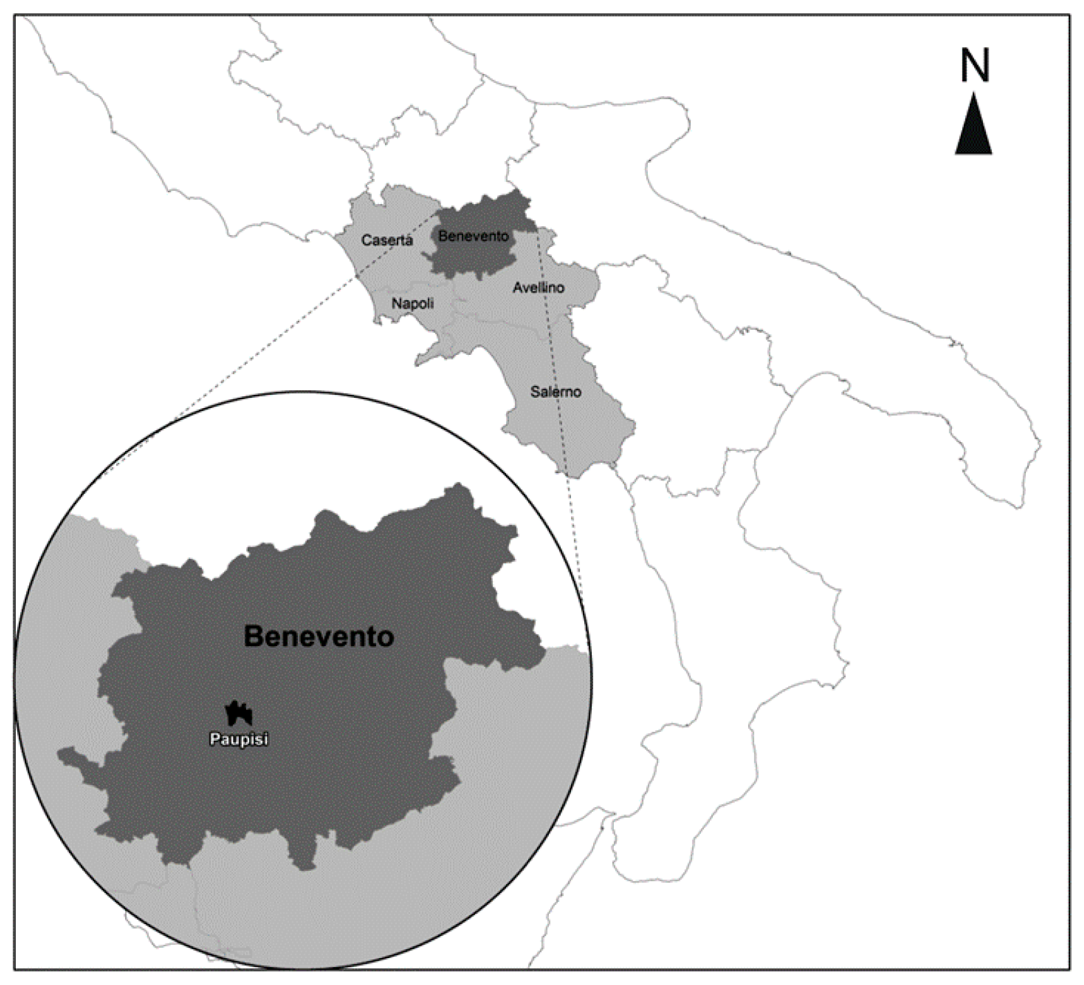
The study area is located upslope of the municipality of Paupisi, in the northern sector of the Campania region (Southern Italy) (Figure 1). It encompasses the northern slope of the Taburno-Camposauro Massif, up to the flood plain of the Calore River to the north.

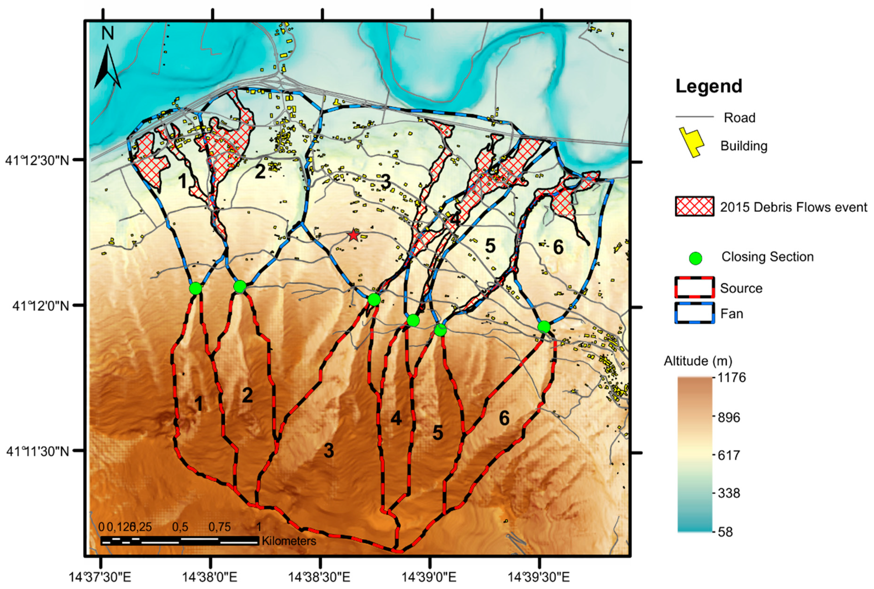
Several catchments prone to debris flows were selected for this study (Figure 2). The geology is characterized by the presence of a Mesozoic calcareous and dolomitic ridge, on which the town of Paupisi is partially built. Limestone slopes are covered by fossil talus deposits and soil alteration, interbedded with paleosols and pyroclastic materials deposited by eruptions of the Somma-Vesuvius. Within the soil mantle and especially in channels, limestone blocks are embedded. The thickness of the cover material range is up 2 m along the slope, while it is almost absent along the watershed. During the night between 14th and 15th October 2015, the area of Paupisi was struck by numerous debris flows triggered by an intense rainfall event [31]. A total rainfall amount of 415.6 mm was recorded in few hours, characterized by a maximum intensity of 27.4 mm/10 min [32]. In this area the average annual precipitation is about 1000–1300 mm [33].

Satellite and aerial images were used to preliminarily map landslide paths that occurred on 14–15 October 2015 (Figure 2). In particular, Google Earth ® images, taken on 4 November 2015 and EROS-B satellite images, taken on 19 October 2015, were compared to obtain the overall fan area affected by both propagation and deposition. Additionally, subsequent field campaigns were carried out to define the limits of the propagation area and define erosion action due to water flow propagation (liquid fraction) on the finer granular fraction of the cultivated fan surface.

2.2. Catchment and Fan Morphometric Features

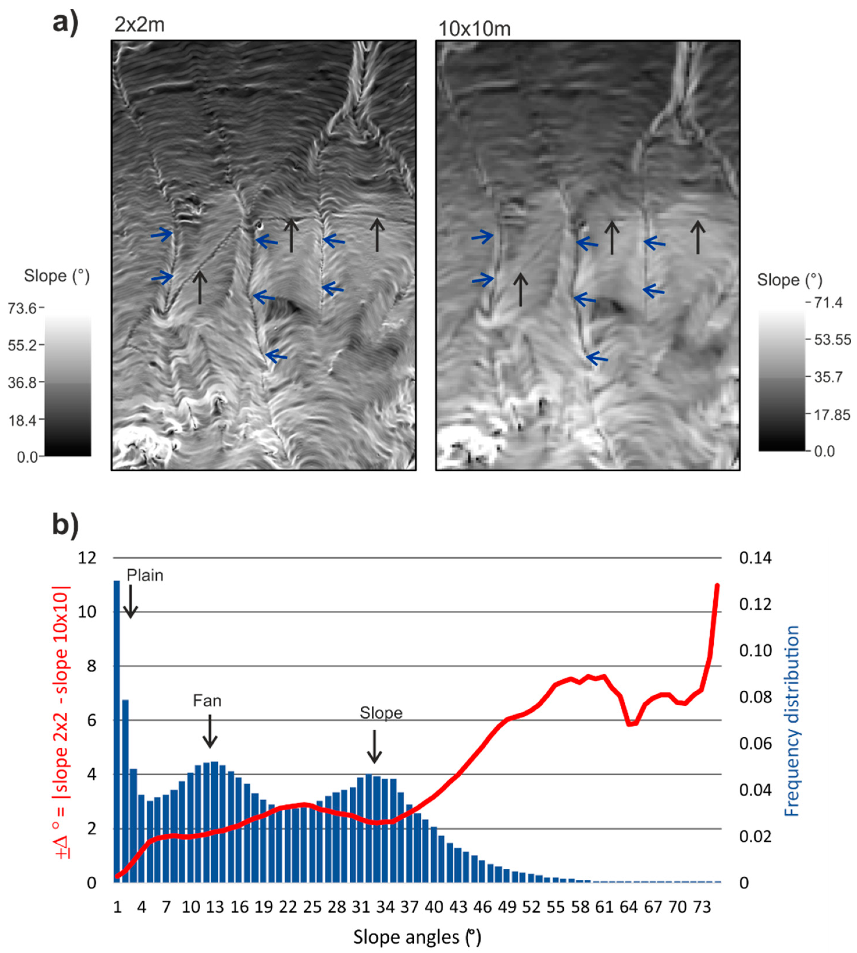
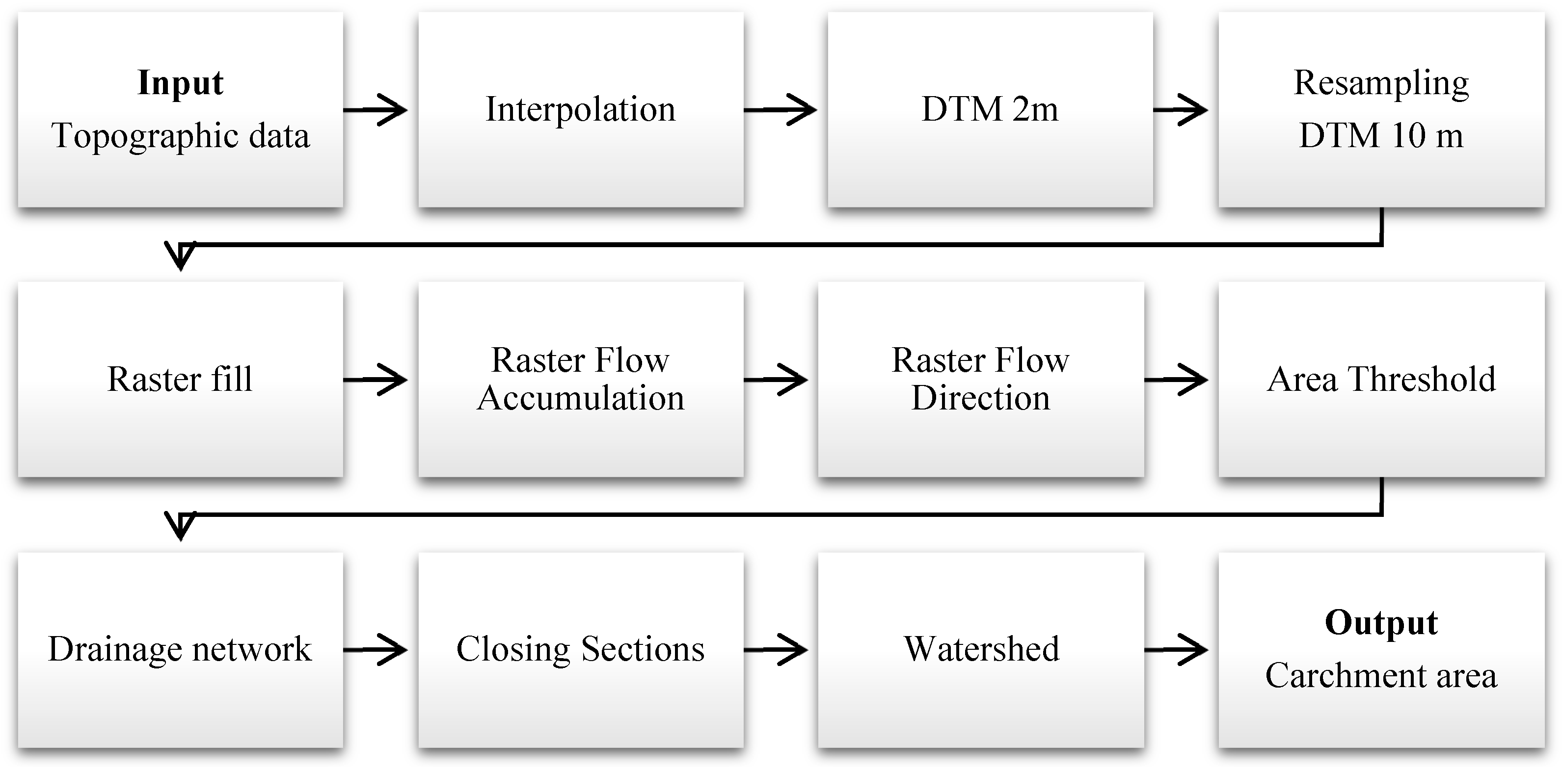
The DEM is the basic geometric model used for the development of the procedure. It was obtained from a 2 × 2 m cell size from vector numerical cartography by using the Topo to Raster interpolation method, specifically designed for the creation of hydrologically correct DEMs. Subsequently, it was resampled by the bilinear interpolation method to a 10 × 10 m planimetric resolution (vertical root mean squared error, RMSE, from 0.21 m to 0.38 m). As highlighted by the Horton et al. [19], this DEM resolution permits a satisfactory compromise between the detail required for the analysis of the hydrographic network and the surface of the study area, in term of roughness attenuation (it increases with lower resolution) and identification of the hydrographic order of channels (it increases with higher resolution) (Figure 3a). In the proposed procedure, slope angle plays a key role in detecting the hydrological pattern, as well as the erosional and depositional areas. In fact, the slope angle frequency distribution shows a multimodal shape in relation to the different sectors of the study area, as follows: 1) alluvial plain (0–5°), 2) fan area (5–22°) with a max frequency of 13° and 3°) slope area (> 22°), with a max frequency ranging from 33–35° (Figure 3b). Such a distribution highlights that error resulting from resampling increases with slope angles. However, by considering a cell resolution of 10 m, the absolute error is very small on a flat area and is within 2° for a slope angle of up to 40°; for slope angles over 40°, a high non-linear increasing of the error occurs.

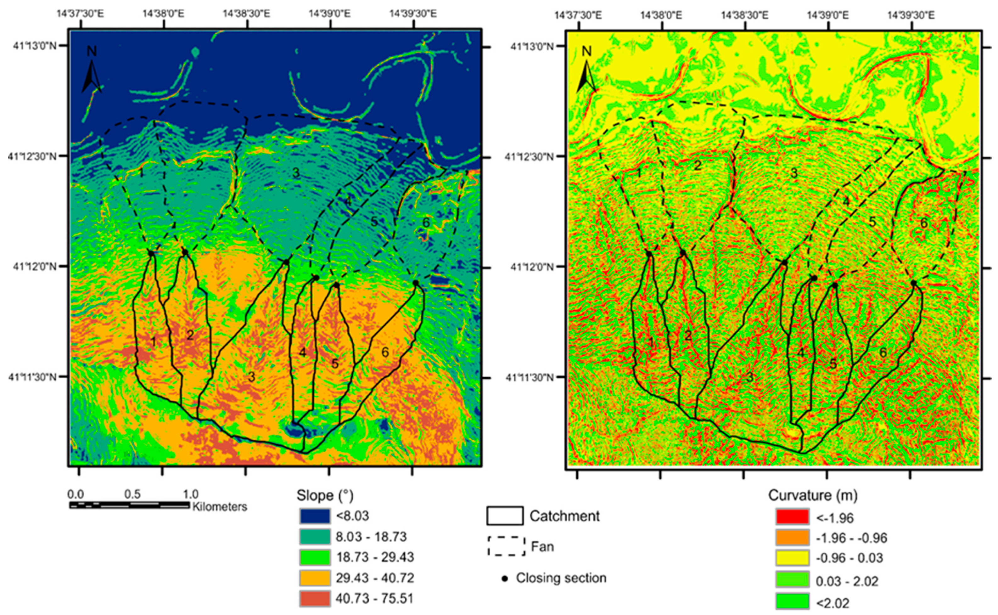
The input data of the proposed procedure are: (1) the DEM-derived maps, which are the Slope map, computed as a gradient of the DEM surface and the Curvature map, computed as a gradient of the slope surface (Figure 4) and (2) the morphometric parameters of the selected basin-fan systems (

Table 1. Morphometric parameters computed for the basins.

CATCHMENT		1	2	3	4	5	6
Area	[m2]	281,945	338,058	741,880	189,398	335,058	270,032
Perimeter	[m]	2967	3141	4260	2668	3253	2975
Length	[m]	1310	1406	1510	1230	1434	1356
Max Altitude	[m]	1120	1175	1177	1103	1153	1064
Min Altitude	[m]	349	353	357	378	378	294
Average Altitude	[m]	764	731	858	761	821	659
Height of relief	[m]	771	822	819	725	775	770
Max Slope	[degree]	75.1	67.0	73.6	63.5	6.9	63.4
Min Slope	[degree]	0.9	1.6	0.1	0.7	0.6	0.6
Average Slope	[degree]	35.3	35.5	34.1	34.5	31.9	33.6
Elevation Relief Ratio	-	0.54	0.46	0.61	0.53	0.57	0.47
Form Factor	-	1.56	1.51	1.38	1.72	1.57	1.60
Drainage Intensity	[1/km]	17.66	14.64	16.82	15.25	15.91	15.09

,

Table 2. Time of concentrations for the six catchments computed using several empirical relationships. A_b, projected basin surface area (km²); Ls, length of the main stream (km); Hm, altitude at the closing section (m a.s.l.); H_MAX, maximum altitude of the catchment (m a.s.l.); H_MIN, minimum altitude of the catchment (m a.s.l.); M and d, numerical dimensionless constants depending on soil type and permeability; for the present analysis we assumed M = 0.20 and d = 0.81; i, average slope gradient of the of the main stream; i_m, average slope gradient of the catchment.

Empirical Relationships	Catchment
	Time of Concentration at the Closing Sections (Minutes)
	1	2	3	4	5	6
$T_c=\frac{\frac{1}{M d}\sqrt{A_b}+1.5{\mathrm{Ls}}_{}}{0.8\sqrt{H_m}}$ [34]	23.00	15.99	31.39	22.66	20.86	22.40
$T_C=0.055\frac{{\mathrm{Ls}}_{}}{\sqrt{i}}$ [35]	6.34	4.19	8.66	6.23	5.65	7.03
$T_C=\frac{ Ls}{3.6}$ [35]	22.63	15.90	28.83	23.35	21.22	24.83
$T_c=0.396 \frac{Ls}{\sqrt{i}}\left(\frac{A_{b } \sqrt{i}}{L{s}^2 \sqrt{i_m}}\right)$ [35]	5.69	5.58	12.13	6.66	6.08	6.60
$T_c=\frac{24·0.045·\sqrt[3]{A_b Ls}}{\sqrt{i}}$ [35]	6.56	4.87	10.68	6.80	6.20	7.35
$c=\frac{0.95 L{s}^{1.155}}{{\left(H_{MAX}-H_{MIN}\right)}^{0.385}}$ [36]	6.28	4.28	8.11	6.35	5.83	6.98
$Tc=0.1272 \sqrt{\frac{A_b}{i}}$ [35]	5.61	4.42	9.97	5.98	5.45	6.31
Average values	10.87	15.99	31.39	22.66	20.86	22.40

and

Table 3. Morphometric parameters computed for the fans.

FAN		1	2	3	4	5	6
Area	[m2]	381,956	665,369	1,010,130	250,121	355,342	369,726
Perimeter	[m]	2822	3405	4206	3190	3329	2540
Max Altitude	[m]	348	357	363	382	381	298
Min Altitude	[m]	67	71	73	84	73	77
Average Altitude	[m]	153	150	168	192	201	183
Height of relief	[m]	280	285	291	298	308	221
Max Slope	[degree]	55.43	60.27	65.03	43.59	67.38	66.93
Min Slope	[degree]	0.02	0.01	0.01	0.26	0.18	0.18
Average Slope	[degree]	12.95	12.16	12.52	11.75	13.82	16.22
Melton’s index (R)	-	1.45	1.41	0.95	1.66	1.33	1.48
Curv. Plane Min	-	−50.25	−46.85	−44.58	−31.17	−65.34	−70.53
Curv. Plane Max	-	33.61	37.31	61.06	28.77	63.65	60.63
Curv. Plane Average	-	−0.03	0.00	0.04	−0.05	0.16	−0.10

). The DEM-derived maps and the morphometric parameters were extracted using GIS geomantic techniques.

The procedure for river basin extraction applied to the study area led to the identification of six catchments and related fans exposing NNE (Figure 2). As shown in Table 1, the basins are located at an average altitude of 766 m a.s.l. (height ranging between 294 and 1176 m a.s.l.) and show an average difference in height of 780 m (difference ranging between 725 m and 822 m). The mean slope angle is 34.2° (data ranging from 31.9° to 35.5°).

Some morphometric parameters were obtained using known empirical laws. More specifically, the hypsometric analysis permitted definition of the Elevation Relief Ratio, ERR, by using the following equation:

$$ERR=\frac{Z_{mean}-Z_{min}}{Z_{max}-Z_{min}}$$

(1)

where Z_max, Z_mean and Z_min are the maximum, average and minimum altitude of the basin. This parameter is tightly related to the morphometric erosional evolution of the catchment and reflects the stages of youth, mature or old [37]. The basins analysed, although having a poorly stratified or massive limestone and calcareous-conglomeratic bedrock, have a calculated ERR ranging between 0.46 and 0.61. The value of ERR shows that they are subject to a medium-high erosion activity and their relief can be classified as ranging between youthful and mature [37].

In addition, the Horton’s relationship [38] was used to calculate the Form Factor:

$$HSF=\frac{A_b}{L_S^2}$$

(2)

where A_b is the projected basin surface area and L_S is the length of the main stream. The Shape Factor ranges between 3.0 and 5.2 and reveals that the basins have an elongated shape, which is an important factor in terms of hydrological response because it influences the time of concentration at the closing sections. Strictly connected to flow phenomena, the time of concentration is computed by using different empirical laws validated in mountain areas (see Table 2). Therefore, the time of concentration, Tc, computed at the closing sections shows an average range of 8–16 min in relation to the length of the basin, rather than its surface (Table 2).

Finally, the Drainage Intensity, DI, was defined as [38]:

$$DI=\frac{LD}{A_b}$$

(3)

where LD is the total length of the hydrographic streams and A_b the drainage surface of the basin described above. The high drainage density values reflect the low permeability of the outcropping soils and the high erosive activity.

Alluvial fans (Figure 4, Table 3) are larger than the corresponding catchments and are located at an average altitude of 174 m a.s.l. (height ranging between 68 and 382 m a.s.l.). The average slope angle is 13.2° with values ranging from 11.7° to 16.2°. The fans consist mainly of limestone gravel in a silty sandy matrix, deposited in the lower-middle Pleistocene. The heterogeneous nature of the fan material will be carefully discussed in Section 2.4.

2.3. Synthetic Hydrographic Network and Catchment-Fan System

Starting from the basic information provided by the digital topography, it was possible to map key parameters of the hydrological processes connected to slope morphometry [39].

The DEM obtained was first corrected for local height anomalies [40]; subsequently, it was possible to define the flow directions according to the path identified by the topographic gradient. The topographic connection of each raster cell allowed creation of a raster of the flow direction using the D8 model [41], which assigns to each cell one of the eight likely flow directions according to the maximum slope direction (E, N, W, S, NE, NW, SW, SE).

The raster of accumulated flows [40,41,42,43,44] represents, for each cell, the cumulative weight of the overhanging area. Cells have a value equal to 1 at the watershed; the cell at the closing section (outflow) is equal to the sum of all the cells of the whole catchment. The definition of a threshold value (Threshold Area) allows filtering of the grid of the drained area by discriminating the cells with values below the threshold (slope cells) from those with higher values (hydrographic network cells).

A value equal to 40,000 m² was given for this specific area, allowing us to obtain a drainage network that is congruent with the size of the single basin (less than 10,000 m²). In this way, the hydrographic network that is defined is comparable with the national official hydrographic network. A univocal value equal to 1 was assigned to the cells with a Flow Accumulation value greater than the threshold value, which were considered as cells of the hydrographic network; a value equal to 0 was assigned to the remaining slope cells. Once the closing section for each basin below the last tributary river segment is identified, it is possible to calculate the extent of the contributing basin by using GIS analysis, which identifies basins and fans as singular independent hydrogeological entities.

Deposition areas were defined by qualitative interpretation of the typical morphological shapes of fans. More specifically, limits of the alluvial fans were assumed to lie at the sudden variation of the topographic gradient.

Definition of the geometrical boundary of the basin-fan systems gave rise to a cluster of polygons used as a basis for the calculation of the morphometric and hydrographic variables by using different GIS tools (Figure 5). These parameters represent important data to discriminate the type of deposit that is predominant in fans [45].

2.4. Event Characteristics and Type of Sediment Transport

The main morphometric parameters of catchments and fans required for the identification of the type of sediment transport process (stream flow, mixed, debris flow) were defined using an indirect method [46,47]. This method defines the type of flow events expected for alluvial fans in relation to the average fan slope and to the Melton’s roughness index, R. This index is defined by the ratio between the difference in height of the highest point in the drainage basin with respect to the fan apex and the square root, HR, of the catchment area, Ab [48]:

$$R=\frac{{\mathrm{H}}_{\mathrm{R}}}{\sqrt{{\mathrm{A}}_{\mathrm{b}}}}$$

(4)

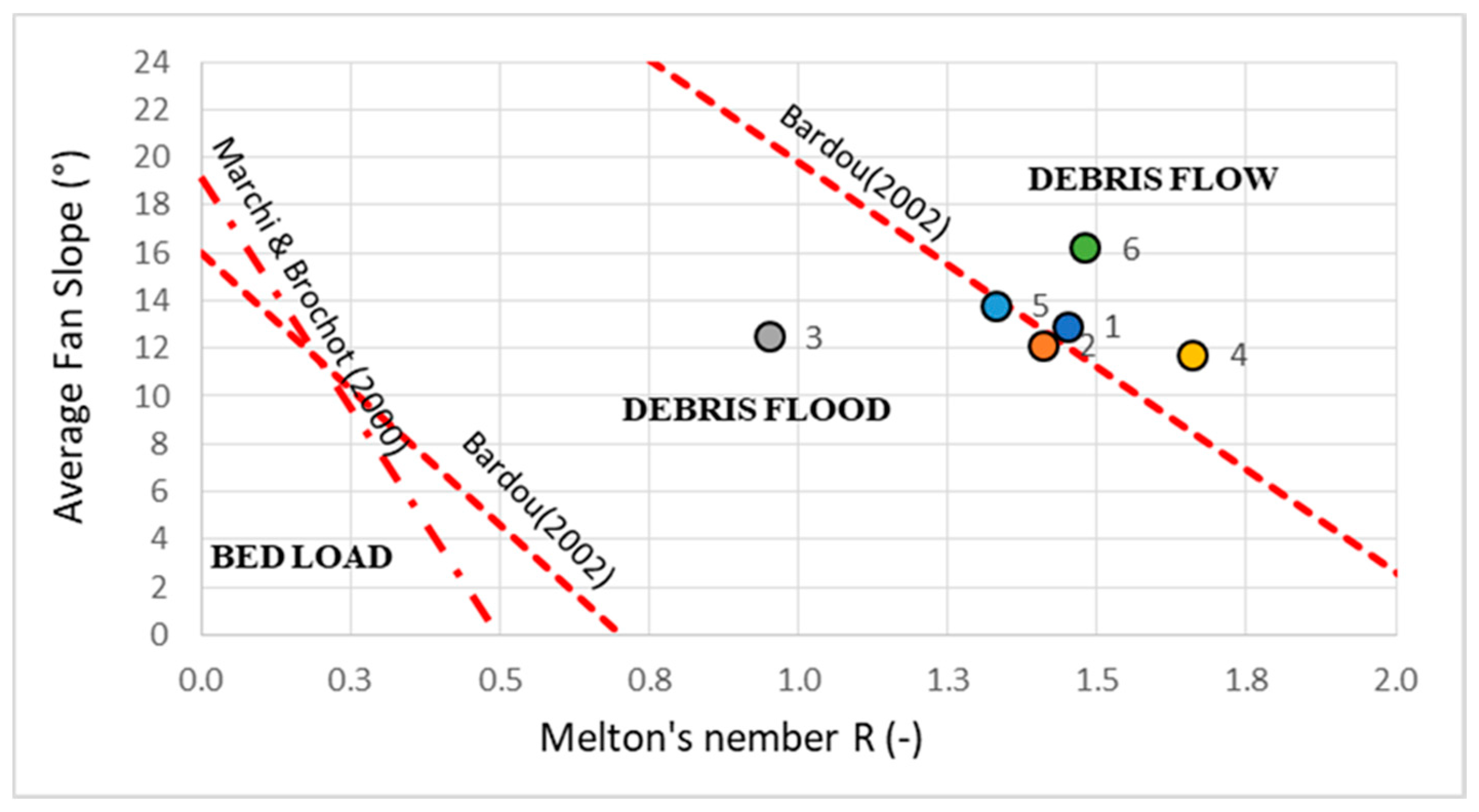
Knowledge of the prevailing sediment transport type allows information to be obtained on the relative intensity of alluvial events that produce debris flows in small-scale mountain basins. This approach, supported by geomorphic or sedimentologic evidence, was applied by Marchi et al. [46] on fan systems in the Dolomites. Others [47,49] have used the same approach in several valleys of the eastern Alps, confirming the morphometric observations with historical observations of high-intensity events. In this way, it is possible to identify those fans mainly exposed to debris flows, which represent the basins potentially more prone to intense alluvial events. The application of the morphometric method proposed by Marchi et al. [46] and experimented with by several authors [50,51,52,53], made it possible to highlight the correlation between the average slope of the fans and the Melton’s index for the studied basins and the predisposition to generate debris flow events (Figure 6). Additionally, following suggestions by Wilford et al. 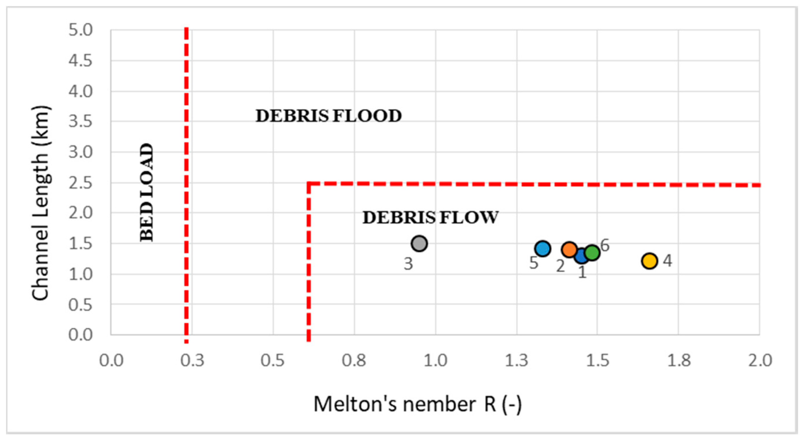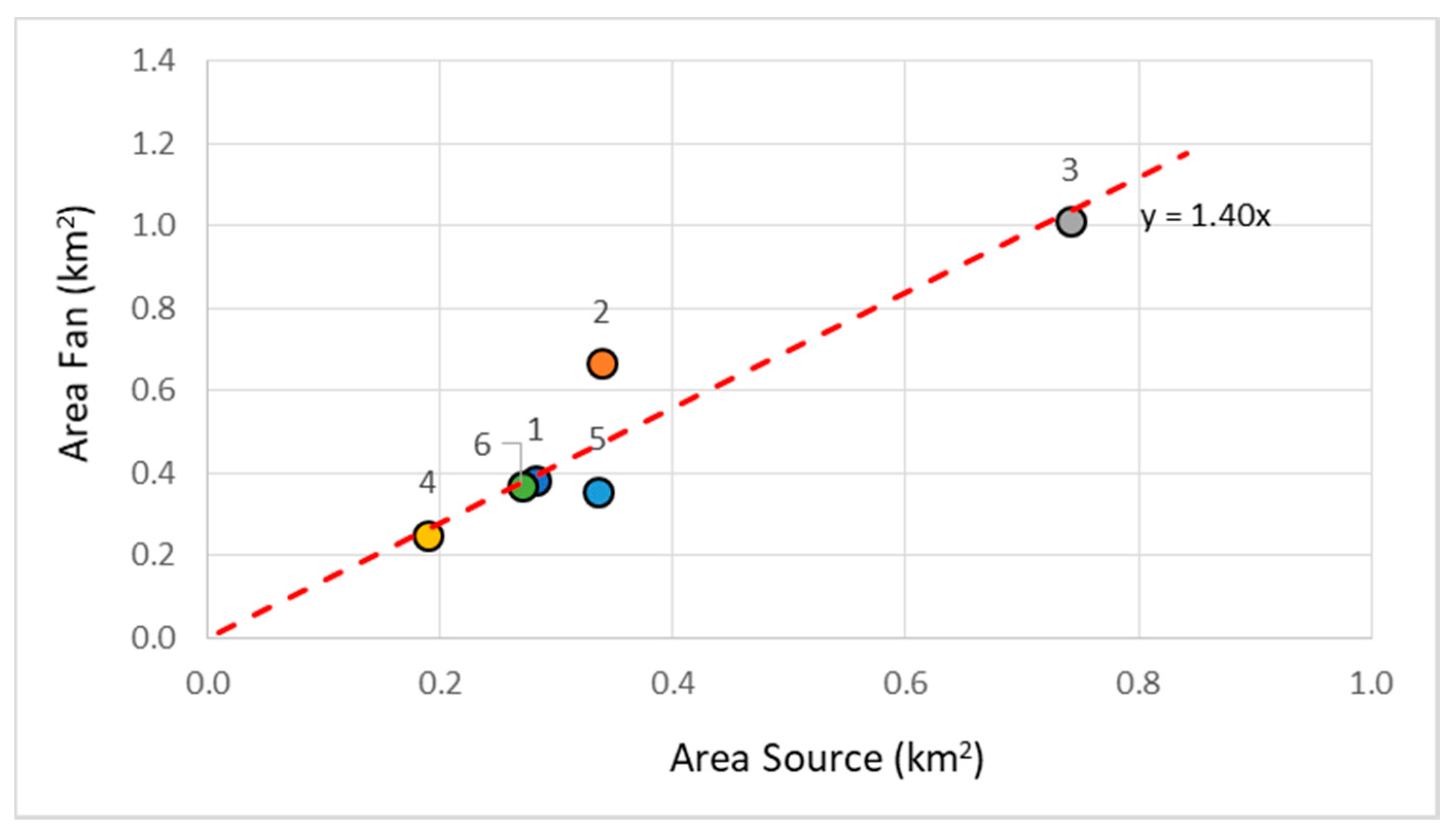[54], the length of basins was found to be related to their respective Melton’s index values (Figure 7), giving analogous results. In addition, the ratio between source area and related fan area shows a common linear relationship which reveals that the fan area is 1.4 times greater that the source area (Figure 8). It should be noted that, in this area, elongation of the foot of fans is generally controlled and prevented by erosion of the Calore River.

With regards to the nature of the fan, field observations and surveys of stratigraphic sequence outcroppings pointed out the repetition of deposits with different grain size distributions for all the fans. In particular, coarse layers are almost always interbedded with silty-sandy deposits consisting of volcanic-ash debris and ancient paleosoils. Analysis of fan materials was defined considering both the phenomena which recently occurred and the sequences of progressive accretion, which contributed to the alluvial fan build-up. As a representative of the whole fans, sampling was performed on a 4.00 m in height cut slope into the fan n° 3 (see Figure 2 for location), where a typical depositional sequence can be considered common to the other nearby fans (Figure 9). The stratigraphy of Figure 9 shows that recurrent extreme flow events could be responsible for the coarse layers present at the top and at the middle-bottom of the analysed sequence and mainly consist of calcareous debris and blocks from bedrock. Other less coarse deposits, consisting of varying thicknesses of pyroclastic soils and pyroclastic debris flows, were interbedded following the main eruptions of both the Somma-Vesuvius and the Phlegrean Fields volcanoes that affected the region at about 10,500 and 3500 years B.P. [57]. In addition, thin layers of colluvium and slow gravity sediment flow are also present, following relatively quiet periods of deposition.

In order to define the specific geotechnical properties of the material forming the stratigraphic sequence of Figure 9, soil samples were taken for each soil layer and tested. More specifically, 15 samples of the exposed cut and 3 samples from a vertical pit excavation were collected. Index properties and mechanical characterization of the coarser layers were carried out on a fraction less than 20 mm in size (

Table 4. Soil profile and geotechnical parameters of the stratigraphic sequence in Figure 8. Particle identification: GwS, gravel with sand; SwGS, silty sand with gravel; GwSS, silty gravel with sand; SlG, low gravelly sand; SwG, sand with gravel; S, sand; SSA, clayey-sandy silt; GwSwS, gravel with silt with sand; SwSGlC, low clayey and low gravelly silt with sand; GS, sandy gravel; SSlC, low clayey sandy silt; SSL, silty sandy gravel.

Sample	Height/Depth Range from Ground Level (cm)	Layer Thickness (cm)	Particle Identification	Unit Weight γs (kN/m3)	Dry Unit Weight γd (kN/m3)	Void Ration e (−)	Friction Angle φ (°)	Water Content w (%)	Carbonate Content CaCO3 (%)
C15	>400	−	GwS	24.7	10.6	1.34	38.2	10.76	8.22
C14	340–400	60	SwGS	24.7	9.0	1.75	none	23.63	7.91
C13	295–340	45	GwSS	23.7	10.2	1.32	none	28.07	5.17
C12	260–295	35	SlG	24.9	10.0	1.50	none	28.14	0.09
C11	235–260	25	SwG	24.6	9.5	1.58	28.5	34.6	0.38
C10	190–235	45	SwG	24.6	17.4	0.41	none	12.01	2.14
C9	178–190	12	S	23.2	9.1	0.98	30.1	52.88	0.06
C8	168–178	10	GwS	23.1	4.6	4.06	none	87.7	0.64
C7	160–168	8	SlG	22.0	8.6	1.55	none	58.28	0.80
C6	148–160	12	SSA	24.1	10.8	1.23	none	35.8	6.50
C5	110–148	38	GS	24.0	11.3	1.13	none	9.53	36.45
C4	80–110	30	GwSwS	25.2	11.0	1.29	none	22.8	17.34
C3	50–80	30	GwSS	24.5	12.9	0.90	none	14.08	10.26
C2	40–50	10	SwSGlC	25.3	10.5	1.40	none	36.30	10.26
C1	0–40	40	GS	25.1	13.3	0.88	34.2	12.01	55.98
B0	−80	80	SSlC	23.4	8.1	1.88	none	50.62	3.23
B1	−80–180	100	SSL	25.2	13.0	0.95	none	11.76	14.32
B2	−180–230	50	SSlC	24.3	9.3	1.62	none	51.56	1.88

). A procedure for the analysis of the grain size distribution of coarse gravels and boulders was utilized for the more superficial layer (C15 sample), deposited before the event of 14–15 October 2015 (Figure 9). This procedure provided for digitalization on photos, by means of polygons of the boundary for the larger particle size fraction (Figure 9). The photos were appropriately scaled by means of a metric target. Polygons were converted into circles of equal area and then to equivalent spheres. The diameter distribution of these equivalent spheres was related to a virtual percentage passing by weight, considering for these soils a unit weight of γ_s, of 24.5 KN/m³ was assumed as an average value of gravel deposits sampled within the depositional sequence (Table 3). Comparison with field surveys and all the laboratory tests indicates that the total grain-size distribution of this deposit can be considered as representative of all deposits originating from stony debris flows, included the event of 14–15 October 2015. The resulting grain-size distribution permitted evaluation of the average value of the friction angle, which is representative of the material, ranging between 38° and 43°. This range defines friction angles slightly greater than those found for sandy granular deposits in Table 4 and matches with the modal slope angle range of the slope surfaces (Figure 3).

2.5. Semi-Automatic Procedure for Debris Flow Dynamics

Debris flows tend to affect inter-mountain catchments rarely exceeding an area of 10 km² [58], involving drainage system formed by narrow valleys and gullies. There are several factors that influence sediment dynamics along the hydrographic network but one of the main roles is played by the topographic setting of the slopes. According to several authors [59,60], topographic parameters that combine the extent of the sediment source areas that can feed debris flows and the local slope angle are able to identify, in the DEM of a basin, the possible initial points of channels of the hydrographic network. In particular, the sediment source area and the local slope angle can be considered as main parameters in debris flow triggering and their erosive capacity.

With regards to the proposed procedure, identification at the basin scale of likely erosion and deposit areas of debris flows is based on the analysis of raster maps derived from the flow chart in Figure 10. In particular, the definition of the trigger zones is defined through a GIS procedure based on the spatial distribution of three parameters: the trigger ratio, TR; slope ratio, SR; and catchment surface, A. Unlike SR and A, which can be obtained by normal GIS procedures, TR is calculated as the ratio between SR and ST, which is the slope threshold. ST (defined in terms of m/m) is given by the following relationship [60]:

$$ST=k A^{-0.2}$$

(5)

where A is the catchment surface in km² and k is a coefficient influencing the model sensitivity [61,62]. It depends on rainfall and the shear strength of soil, plus the contribution given by the vegetation root system [60]. This approach is based on the fact that, in the presence of sediment available to be mobilized, debris flow development and propagation depends on (1) overcoming of the critical values of water discharge and (2) slope angle of the channel.

The analysis is implemented with a semi-automatic procedure within the Raster Calculator tool. Following the equation proposed by Zimmermann et al. [61], the conversion of the A’s raster in square kilometres was carried out. For the application of the procedure in the study area, different values of k and therefore of ST were used. As reported by Wichmann et al. [62], the choice of k plays a key role in the distribution of the erosion along the hydrographic network within the source areas. The spatial recognition of likely triggering points is defined as the product of the binary mask values (e.g., 1 = yes and 0 = no) obtained by combining the fields of existence in

Table 5. Raster masks for erosion prediction.

Switch on/off Raster	Value	Mask Value
Catchment surface	≤10 km2	1
Catchment surface	>10 km2	0
Slope	≤38°	1
Slope	>38°	0
Trigger ratio, TR	≥1	1
Trigger ratio, TR	<1	0

. The mask of the catchment surface ≤ 10 km² assigns a value equal to 1 to all pixels with an area less than 10 km² and a value equal to 0 to pixels with areas greater than 10 km². High values of the drained area are usually linked with solid transport processes at the bed and suspended [58]. The slope mask ≤ 38° gives a value of 1 to all cells with a slope angle less than 38° and a value of 0 to cells with slope angle greater than this value.

For a local slope angle greater than 38°, which is a value close to the internal frictional angle of debris materials often present in the source areas’ debris flows, the amount of debris material that can be mobilized is considered modest or negligible. These areas are therefore excluded from the likely triggering zones of debris flows [26]. The trigger ratio mask R ≥ 1 assigns a value of 1 to cells with slope angles greater than or equal to the slope threshold ST and a value of 0 to those that have an R less than one. Areas prone to debris flow initiation are obtained through the product of the mask values of the above fields of existence, which depend on the depositional characteristics of past phenomena and on the specific features of the study area. Moreover, in order to take into account the depositional attitude in relation to the surface convexity (positive values) or concavity (negative values), the parameter curvature was used as a further discriminating factor for the identification of the deposition areas. Conditions applied for sediment deposition are reported in

Table 6. Raster masks for deposition prediction.

Switch on/off Raster	Value	Mask Value
Slope	≤15°	1
Slope	>15°	0
Slope	>6°	1
Slope	<6°	0
Trigger ratio, TR	≤0.5	1
Trigger ratio, TR	>0.5	0
Curvature plane	<0.1	1
Curvature plane	≥0.1	0
Curvature plane	>−0.3	1
Curvature plane	<−0.3	0

.

In this study, susceptible deposit areas were identified on the base of slope angles ranging from 6 to 15°, as inferred by comparison with the 2015 events and with previous studies investigating the relationship between slope angle and debris flow runout and deposition. In particular, Prochaska et al. [63] identified the propagation phase on the fan area in reference to a slope angle ratio equal to 0.88, which is computed between the debris flow’s runout angle and slope angle at the closing sections. Therefore, assuming in these sites a minimum slope angle of 18° (Figure 2), it follows that runout without deposition is always possible for slope angles higher than 15°. The slope angle range for deposition prediction is selected in the procedure by using two different binary masks (Table 6). In addition, several others binary masks are associated with a trigger ratio, TR, greater than 0.5, which takes into account propagation without deposition. Finally, curvature values ranging from –0.3 to –0.1 detect the poorly convex and concave depressions that are not associated with channel shape conditions (curvature < –0.3).

3. Results

The procedure previously described permitted introduction of a semi-automatized GIS-morphometrical model able to estimate erosion and deposition areas due to canalized water flow that may develop into debris flow responsible for fan accretion.

With regards to the prediction of the debris flow initiation areas (Figure 11), defined as areas of the channel bed subject to intense erosion, we used values of k (Equation (5)) equal to 0.20, 0.28, 0.32 and 0.36, selected after model sensitivity analysis, in order to evaluate the influence of this parameter on model results. In reality, as shown in Figure 11, variation of k influences the extent of the involved channel area and consequently the likely erosion area within the hydrographic network. Generally, a decrease of k leads to an increase of the debris flow initiation areas towards upstream; moreover, a non-linear persistence of the erosional phenomenon in the main channels occurs when k increases. Therefore, an evident decrease (about 50%) of areas involved in channel bed erosion is observed for k = 0.20 and k = 0.28; further decreases of these values have a minor influence on the distribution of the erosion channel areas (Figure 11). In qualitative terms, from field observations and aerial and satellite images, it seems reasonable that the debris flows of 14–15 October 2015 can be simulated with an intermediate value of k. In this regard, it should be noted that an extensive dendritic pattern of erosion crossing the hydrographic networks was not observed from areal and satellite images. Conversely, field surveys highlighted that the main channel showed several areas subjected to erosion that could be successfully modelled by using k values between 0.28 and 0.32. This means that the model estimated a range between 15–21% of the basin drainage channel, respectively, as erosion areas.

Deposition areas identified by the application of this procedure must be considered as areas of potential accumulation of material transported downstream during high intensity storms. The prediction of these areas is entirely based on morphometric factors and, therefore, is independent from the characteristics of the flow event and the amount of debris mobilized. The distribution of the deposition areas predicted by the procedure overlaps almost entirely the existing fans, assuming an apical arrangement and splitting from the basin closing sections (Figure 12). Coherently, deposition areas within the catchment domain are not predicted in any cases. Deposit distribution on the fan surface is discontinuous, highlighting material concentrations along flow directions constituted by morphological depressions. Non-deposit areas are identified along banks of deepened channels and in areas of specific convergence of slope surface steepness and convexity.

4. Discussion

In addition, as defined in Table 5, the trigger ratio (TR) is a relevant value in prediction that increases fan depositional areas. In general terms, when TR increases (increasing the k value), a higher number of cells pass under the 0.5 value, even though the predicted areas are always obtained by a combination of these cells with others that are defined by the slope and curvature thresholds. 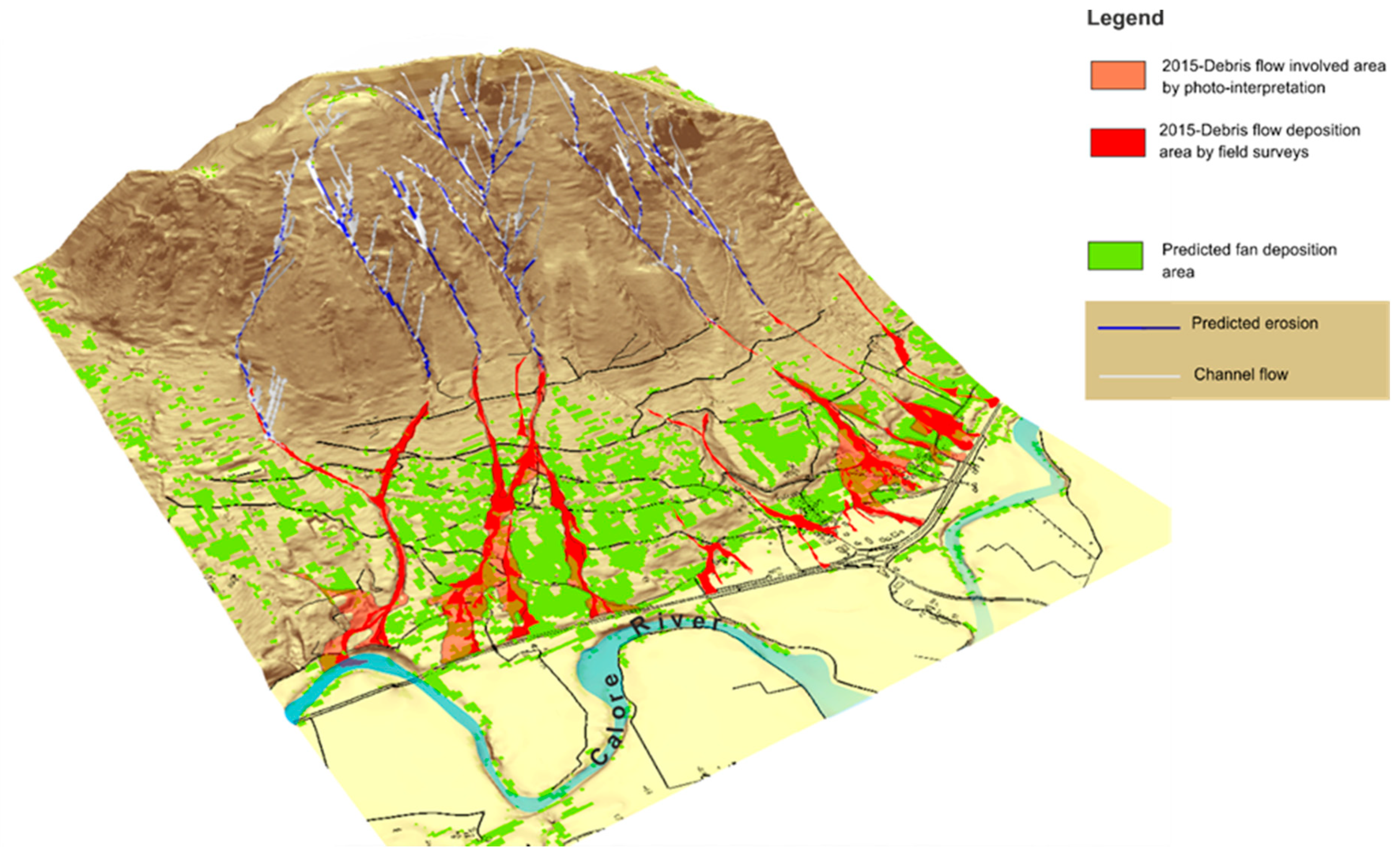This latter aspect produces a non-linear relationship between the predictable areas of deposition and the k values, as inferred from the graph of Figure 11. In addition, for the deposition areas, variation of the k parameter does not increase the extension of the deposit itself but as k increases, a localized growth of deposit area density occurs (higher point density within the same area unit). This effect is more evident compared with the depositional area of the 2015 debris flow events mapped by the field survey. In this case, due to the k increase, the depositional area increase intensifies the positive prediction of cells, mainly into the already predicted areas. A comparison of the 2015 debris flow deposition mapped by the field survey shows that about 62% of the deposit matches the model results by using k = 0.32, without considering the channel area on the fan. Conversely, including the larger invasion area detected by photo-interpretation, comparison with the model results gives the result of 46% matching (Figure 12). Moreover, the model results on fans #3 and #4 show a concentration of deposits strongly localized in a zone which is not aligned with the axis of the main channel and with the fan geometry. This area experienced a larger invasion and deposition of the actual debris flow event.

The preliminary GIS analysis permitted characterization in terms of type of evolution of the basin-fan systems of the study area. First, the Melton’s index was used to classify the flow events responsible for fan accretion. Analyses of fan stratigraphic sequences and materials from a cut slope and an excavated pit confirmed the main event types of slope evolution, consisting of stony debris flows and pyroclastic or mixed debris flow in relation to the regional volcanic activity. Second, the Elevation Relief Ratio, ERR, highlighted medium-high erosion activity and catchments which can be classified as ranging between youthful and mature. In addition, an average time concentration ranging between 7 and 15 min can be assigned to the basin areas in relation to their extensions, rather than their elongations.

Subsequently, the proposed procedure, mainly based on morphometric DEM-derived parameters, was applied to estimate basin channel areas prone to erosion and fan areas prone to deposition as a result of debris flow events. Both these areas were detected without considering the magnitude of the triggering rainfall events, the material volume involved and its rheological characteristics.

The procedure allowed the definition of the hydrographic network for each selected basin and the potential erosion and deposition area, in an automated way. For application at the study area, it required the extraction of several key map parameters, such as the trigger ratio, TR and other specific DEM-derived maps (e.g., Slope and Curvature). All these maps were switched-on and switched-off in specific range values by binary raster masks. Particularly, it was possible to find that the values of the k parameter controlled the TR’s influence on the extension/density of the erosion and deposit predicted areas in the opposite way. By considering this influence, a parameterized analysis by changing the k values was performed. It results in k assuming a non-linear relationship with the area detected both for erosion and deposition and in particular:

k_D = 0.5 (1 − k_S)

(6)

where k_D and k_S are the k values used in the depositional and erosion modelling, respectively.

Considering such a k-trend, it was possible to define that general modelling for prediction of erosion of depositional areas can be carried about by using different values of k. Figure 13 shows an overall view of the procedure applied at the study area, compared with the 2015 debris flow, by using k_D = 0.36 and k_S = 0.28. Qualitative-quantitative comparison with the model output revealed that a range of 15–21% of the depositional area is computed for the six-fan area. Moreover, in this predicted area falls about 46% of the invasion/depositional area of the 2015 debris flow event detected by photo-interpretation and 62% of the depositional area detected by field investigation. Most of the unpredicted areas were related to the head of the debris flow that had reached the alluvial plain of the Calore River. This river exerts a control action on the distal limit of the fan due to the progressive erosion of material that has reached the fan base. A marker of this morphological control is a border escarpment that joins the fans with the river plain (Figure 13).

It should be noted that this procedure, similarly to other recently-proposed GIS-based models [19,20,30], presents some limitations related to the empirical character of the morphometrical and morphological criteria used. As a matter of the fact, despite one of the main advantages of the procedure being its easy applicability and reproducibility due to the limited input data required from DEM alone, it does not consider specific aspects related to debris flow triggering, such as features of the storm event and material properties, such as rheological parameters. Moreover, debris volume available or transported and debris flow velocity or energy are also not considered.

5. Conclusions

A simplified GIS-based procedure for assessing areas exposed to debris flows is presented in this study. The morphometric nature of the proposed GIS computational model means that it can be considered as a quick and easy tool for preliminary estimation of potential erosion and deposition area into channels and along alluvial fans. It should be noted that the model aims to estimate areas prone to being eroded or deposited, rather than areas that will be involved in a probabilistic debris flow event. Prediction of the latter requires complex multiparametric computational models, which should be based on the physics of the phenomenon and also on the probabilistic analysis of the rainstorm triggering event, of the thickness of the debris material into the channel and on its geotechnical behaviour during the initial, propagation and deposition phases. However, although this proposed approach can be affected by limitations in prediction, due to the empirical character of the morphometrical and morphological criteria used as for others based on DEM data, it can be used to support the design of susceptibility maps which are preparatory steps for hazard analysis in vast areas.

For the study area, taking into consideration the non-exclusive predictive nature of the model, the comparison of the model results with the actual erosion and deposition areas of the 2015 debris flow showed a good performance of the procedure.

Finally, the identification of (i) key parameters controlling the evolution of the basin-fan systems, (ii) the hydrographic network with respect to erosion and transport areas and (iii) the likely deposit areas can play an important role in zones where information about likely future debris flow events are not available.

References

- Hungr, O.; Leroueil, S.; Picarelli, L. The Varnes classification of landslide types, an update. Landslides 2014, 11, 167–194. [Google Scholar] [CrossRef]
- Revellino, P.; Hungr, O.; Guadagno, F.M.; Evans, S.G. Velocity and runout simulation of destructive debris flows and debris avalanches in pyroclastic deposits, Campania Region, Italy. Environ. Geol. 2004, 45, 295–311. [Google Scholar] [CrossRef]
- Grelle, G.; Revellino, P.; Donnarumma, A.; Guadagno, F.M. Bedding control on landslides: A methodological approach for computer-aided mapping analysis. Nat. Hazard Earth Syst. 2011, 11, 1395–1409. [Google Scholar] [CrossRef]
- Jakob, M.; Hungr, O. Debris-Flow Hazards and Related Phenomena; Springer: Chichester, UK, 2005. [Google Scholar]
- Welsh, A.J.; Davies, T. Identification of alluvial fans susceptible to debris-flow hazards. Landslides 2011, 8, 183–194. [Google Scholar] [CrossRef]
- Skilodimou, H.D.; Bathrellos, G.D.; Koskeridou, E.; Soukis, K.; Rozos, D. Physical and Anthropogenic Factors Related to Landslide Activity in the Northern Peloponnese, Greece. Land 2018, 7, 85. [Google Scholar] [CrossRef]
- Guerriero, L.; Revellino, P.; Grelle, G.; Fiorillo, F.; Guadagno, F.M. Landslides and infrastructures: The case of the montaguto earth flow in southern Italy. Ital. J. Eng. Geol. Environ. 2013, 6, 459–466. [Google Scholar]
- Santi, P.M.; Hewitt, K.; VanDine, D.F.; Barillas Cruz, E. Debris-flow impact, vulnerability and response. Nat. Hazards 2010, 56, 371–402. [Google Scholar] [CrossRef]
- Pierson, T.C. Initiation and Flow Behavior of the 1980 Pine Creek and Muddy River Lahars, Mount St. Helens, Washington. Geol. Soc. Am. Bull. 1985, 96, 1056–1069. [Google Scholar] [CrossRef]
- Takahashi, T. Debris Flows; Balkema: Rotterdam, The Netherlands, 1991. [Google Scholar]
- Hungr, O. A model for the runout analysis of rapid flow slides, debris flows and avalanches. Can. Geotech. J. 1995, 32, 610–623. [Google Scholar] [CrossRef]
- Hurlimann, M.; Rickenmann, D.; Medina, V.; Baterman, A. Evaluation to calculate debris flow parameters for hazard assessment. Eng. Geol. 2008, 12, 152–163. [Google Scholar] [CrossRef]
- Rickenmann, D. Empirical Relationships for Debris Flows. Nat. Hazards 1999, 19, 47–77. [Google Scholar] [CrossRef]
- Revellino, P.; Guerriero, L.; Grelle, G.; Esposito, L.; Guadagno, F.M. Initiation and propagation of the 2005 debris avalanche at Nocera Inferiore (Southern Italy). Ital. J. Geosci. 2013, 132, 366–379. [Google Scholar] [CrossRef]
- Tarolli, P.; Arrowsmith, J.R.; Vivoni, E.R. Understanding earth surface processes from remotely sensed digital terrain models. Geomorphology 2009, 113, 1–3. [Google Scholar] [CrossRef]
- Tarolli, P.; Tarboton, D.G. A new method for determination of most likely landslide initiation points and the evaluation of digital terrain model scale in terrain stability mapping. Hydrol. Earth Syst. Sci. 2006, 10, 663–677. [Google Scholar] [CrossRef] [Green Version]
- Montgomery, D.R.; Dietrich, W.E.A. physically-based model for topographic control on shallow landsliding. Water Resour. Res. 1994, 30, 1153–1171. [Google Scholar] [CrossRef]
- Yin, L.; Zhu, J.; Li, Y.; Zeng, C.; Zhu, Q.; Qi, H.; Liu, M.; Li, W.; Cao, Z.; Yang, W.; et al. A Virtual Geographic Environment for Debris Flow Risk Analysis in Residential Areas. ISPRS Int. J. Geo. Inf. 2017, 6, 377. [Google Scholar] [CrossRef]
- Horton, P.; Jaboyedoff, M.; Rudaz, B.; Zimmerman, M. Flow-R, a model for susceptibility mapping of debris flows and other gravitational hazards at a regional scale. Nat. Hazards Earth Syst. 2013, 13, 869–885. [Google Scholar] [CrossRef] [Green Version]
- Yu, F.C.; Chen, C.Y.; Chen, T.C.; Hung, F.Y.; Lin, S.C. A GIS Process for Delimitating Areas Potentially Endangered by Debris Flow. Nat. Hazards 2006, 37, 169. [Google Scholar] [CrossRef]
- Ayalew, L.; Yamagishi, H.; Marui, H.; Kanno, T. Landslides in Sado Island of Japan: GIS-based susceptibility mapping with comparisons of results from two methods and verifications. Eng. Geol. 2005, 81, 432–445. [Google Scholar] [CrossRef]
- Han-Saem, K.; Choong-Ki, C.; Sang-Rae, K.; Kyung-Suk, K. A GIS-Based Framework for Real Time Debris-Flow Hazard Assessment for Expressways in Korea. Int. J. Disas. Risk 2016, 7, 293–311. [Google Scholar]
- Castelli, F.; Freni, G.; Lentini, V.; Fichera, A. Modelling of a debris flow event in the Enna area for hazard assessment. Procedia Eng. 2017, 175, 287–292. [Google Scholar] [CrossRef]
- Beguería, S.; Van Asch, T.W.J.; Malet, J.-P.; Gröndahl, S. A GIS-based numerical model for simulating the kinematics of mud and debris flows over complex terrain. Nat. Hazards Earth Syst. 2009, 9, 1897–1909. [Google Scholar] [Green Version]
- Mergili, M.; Fischer, J.-T.; Krenn, J.; Pudasaini, S.P. R.avaflow v1, an advanced open-source computational framework for the propagation and interaction of two-phase mass flows. Geosci. Model Dev. 2017, 10, 553–569. [Google Scholar] [CrossRef]
- Iverson, G.R.M.; Schilling, S.P.; Vallance, J.W. Objective delineation of lahar-inundation hazard zones. Geol. Soc. Am. Bull. 1998, 110, 972–984. [Google Scholar] [CrossRef]
- Carrara, A.; Guzzetti, F.; Cardinali, M.; Reichenbach, P. Use of GIS technology in the prediction and monitoring of landslide hazard. Nat. Hazards 1999, 20, 117–135. [Google Scholar] [CrossRef]
- Van Westen, C.J.; van Asch, T.W.J.; Soeters, R. Landslide hazard and risk zonation—Why is it so difficult? Bull. Eng. Geol. Environ. 2006, 65, 167–184. [Google Scholar] [CrossRef]
- Berti, M.; Simoni, A. Prediction of debris flow inundation areas using empirical mobility relationships. Geomorphology 2007, 90, 144–161. [Google Scholar] [CrossRef]
- Cavalli, M.; Crema, S.; Trevisani, S.; Marchi, L. GIS tools for preliminary debris-flow assessment at regional scale. J. Mt. Sci. 2017, 14, 2498–2510. [Google Scholar] [CrossRef]
- Santo, A.; Santangelo, N.; Forte, G.; De Falco, M. Post flash flood survey: The 14th and 15th October 2015 event in the Paupisi-Solopaca area (Southern Italy). J. Maps 2017, 13, 19–25. [Google Scholar] [CrossRef]
- Guerriero, L.; Focareta, M.; Fusco, G.; Rabuano, R.; Guadagno, F.M.; Revellino, P. Flood hazard of major river segments, Benevento Province, Southern Italy. J. Maps 2018, 14, 597–606. [Google Scholar] [CrossRef]
- Grelle, G.; Soriano, M.; Revellino, P.; Diodato, N.; Guadagno, F.M. Space-time prediction of rainfall-induced shallow landslides through a combined probabilistic/deterministic approach, optimized for initial water table conditions. Bull. Eng. Geol. Environ. 2014, 73, 877–890. [Google Scholar] [CrossRef]
- Aronica, I.; Paltrinieri, E. Bonifica Montana nel Comprensorio dell’Alto Simeto; Istituto Poligrafico dello Stato: Rome, Italy, 1954; p. 164. [Google Scholar]
- Viparelli, M. Lezioni di Idraulica; Liguori: Naples, Italy, 1975. [Google Scholar]
- Kirpich, Z.P. Time of concentration of small Agricultural Watersheds. Civ. Eng. 1940, 10, 362. [Google Scholar]
- Pike, R.J.; Wilson, S.E. Elevation-Relief Ratio, Hypsometric Integral and Geomorphic Area—Altitude Analysis. Geol. Soc. Am. Bull. 1971, 82, 1079–1084. [Google Scholar] [CrossRef]
- Horton, R.E. Drainage-basin characteristics. Trans. Am. Geophys. Union 1932, 13, 350–361. [Google Scholar] [CrossRef]
- Cazorzi, F.; Dalla Fontana, G.; Fattorelli, S. GIS capabilities in hydrological studies. TERR@A Brief 2000, 3, 14–17. [Google Scholar]
- Tarboton, D.G.; Bras, R.F.; Rodriguez-Iturbe, I. On the extraction of channel networks from digital elevation data. Hydrol. Process. 1991, 5, 81–100. [Google Scholar] [CrossRef]
- O’Callaghan, J.F.; Mark, D.M. The extraction of drainage networks from digital elevation data. Lect. Notes Comput. Sci. 1984, 28, 323–344. [Google Scholar]
- Martz, L.W.; Garbrecht, J. Numerical definition of drainage network and subcatchment areas from digital elevation models. Comput. Geosci. 1992, 18, 747–761. [Google Scholar] [CrossRef]
- Jenson, S.K.; Domingue, J.O. Extracting topographic structure from digital elevation models. Photogramm. Eng. Remote Sens. 1988, 54, 1593–1600. [Google Scholar]
- Marks, D.; Dozier, J.; Frew, J. Automated basin delineation from digital elevation data. Geo-Processing 1984, 2, 299–311. [Google Scholar]
- Jackson, L.; Kostaschuk, R.; Mac Donald, G. Identification of debris flow hazard on alluvial fans in the Canadian Rocky Mountains. In Debris Flows/avalanches: Process, Recognition, and Mitigation; Costa, J.E., Wieczorek, F.G., Eds.; Geological Society of America: Boulder, CO, USA, 1987; Volume 7, pp. 115–124. [Google Scholar]
- Marchi, L.; Pasuto, A.; Tecca, P.R. Flow processes on alluvial fans in the Eastern Italian Alps. Z. Geomorphol. 1993, 37, 447–458. [Google Scholar]
- Marchi, L.; Dalla Fontana, G. GIS morphometric indicators for the analysis of sediment dynamics in mountain basins. Environ. Geol. 2005, 48, 218. [Google Scholar] [CrossRef]
- Melton, M.A. The Geomorphic and Palaeoclimatic Significance of Alluvial Deposits in Southern Arizona. J. Geol. 1965, 73, 1–38. [Google Scholar] [CrossRef]
- Marchi, L.; Tecca, P.R. Alluvial fans of the Eastern Italian Alps: Morphometry and depositional processes. Geodin. Acta 1995, 8, 20–27. [Google Scholar] [CrossRef]
- Bonifazi, G.; Sappa, G.; De Casa, G. Applications of images digital analysis in the characterisation of grains morphology influence in mechanical behaviour of granular soils. Mater. Res. Soc. Symp. Proc. 1995, 362, 167–172. [Google Scholar]
- Guzzetti, F.; Marchetti, M.; Reichenbach, P. Large alluvial fans in the north-central Po Plain (Northern Italy). Geomorphology 1997, 18, 119–136. [Google Scholar] [CrossRef]
- Sorriso-Valvo, M.; Antronico, L.; Le Pera, E. Controls on modern fan morphology in Calabria, Southern Italy. Geomorphology 1988, 24, 169–187. [Google Scholar] [CrossRef]
- De Scally, F.A.; Owens, I.F. Morphometric controls and Geomorphic responses on fans in the Southern Alps, New Zealand. Earth Surf. Proc. Landf. 2004, 29, 311–322. [Google Scholar] [CrossRef]
- Wilford, D.J.; Sakals, M.E.; Innes, J.L.; Sidle, R.C.; Bergerud, W.A. Recognition of debris flow, debris flood and flood hazard through watershed morphometrics. Landslides 2004, 1, 61–66. [Google Scholar] [CrossRef] [Green Version]
- Marchi, L.; Brochot, S. Mountain torrent alluvial fans in the French Alps: Morphometry and solid flow processes [Les cones de dejection torrentiels dans les Alpes francaises: Morphometrie et processus de transport solide torrentiel]. Rev. Geogr. Alp. 2000, 88, 23–38. [Google Scholar] [CrossRef]
- Bardou, E. Methodologie de Diagnostic des Laves Torrentiells sur un Bassin Versant. Ph.D. Thesis, Ecole Polytechnique de Lausanne, Lausanne, Switzerland, 2002. [Google Scholar]
- Revellino, P.; Guadagno, F.M.; Hungr, O. Morphological methods and dynamic modelling in landslide hazard assessment of the Campania Apennine carbonate slope. Landslides 2008, 5, 59–70. [Google Scholar] [CrossRef]
- Marchi, L.; D’agostino, V. Estimation of debris flow magnitude in the eastern Italian Alps. Earth Surf. Proc. Land. 2004, 29, 207–220. [Google Scholar] [CrossRef]
- Desmet, P.J.J.; Poesen, J.; Govers, G.; Vandaele, K. Importance of slope gradient and contributing area for optimal prediction of the initiation and trajectory of ephemeral gullies. Catena 1999, 37, 377–392. [Google Scholar] [CrossRef]
- Montgomery, D.R.; Foufoula-Georgiou, E. Channel network source representation using digital elevation models. Water Resour. Res. 1993, 29, 3925–3934. [Google Scholar] [CrossRef]
- Zimmermann, M.; Mani, P.; Gamma, P.; Gsteiger, P.; Heiniger, O.; Hunziker, G. Murganggefahr und Klimaänderung—ein GIS-basierter Ansatz; Schlussbericht NFP 31; Hochschulverlag an der ETH: Zürich, Switzerland, 1997. [Google Scholar]
- Wichmann, V.; Becht, M. Modelling of Geomorphic Processes in an Alpine Catchment. GeoDynamics 2005, 20, 151–167. [Google Scholar]
- Prochaska, A.B.; Santi, P.M.; Higgins, J.D.; Cannon, S.H. Debris-flow runout predictions based on the average channel slope (ACS). Eng. Geol. 2008, 98, 29–40. [Google Scholar] [CrossRef]
Figure 1.
Geographic location of the study area.
Figure 2.
Catchments (red-black boundary) and related fans (blue-black boundary) selected for this study and identified by progressive numbering. The red star indicates the position of the sampling site and reconstruction of a representative stratigraphic log of fans.
Figure 3.
(a) Resampling from a 2 × 2 m to a 10 × 10 m cell size DEM: the main hydrographic network (blue arrows) is preserved and the road scarp (black arrows) is smoothed. (b) Slope angle frequency distribution and absolute error distribution from resampling.
Figure 4.
Raster maps of the six basins derived by DEM: (a) Slope; (b) Curvature.
Figure 5.
Flow chart of the hydrology tools.
Figure 6.
Transportation type: Melton’s index vs. average fan slope (modified from Marchi et al. [
46]). Numbered coloured dots correspond to the six catchments. Fields defined by Marchi and Brochot and Bardou [
55,
56] are also shown.
Figure 7.
Transportation type: Melton’s index and channel length (modified from Wilford et al. [
54]). Numbered coloured dots correspond to the six catchments.
Figure 8.
Relation between fans and source areas. Numbered coloured dots correspond to the six catchments.
Figure 9.
Typical grain size distribution of the fan sequence in the study area. Digital-photo analysis for boulders and gravels of the near surface sample and stratigraphic log are also shown. Location of the soil sequence is reported in
Figure 10.
Flow chart of the predictive procedure of trigger and deposit areas.
Figure 11.
Hydrographic network and erosion areas within the channels predicted by the model using different values of k. Red columns are the percentage of the eroded hydrographic network simulated by the model, blue columns are the relative complementary value to 100% of the channel length.
Figure 12.
Deposition areas on fans predicted by the model and compared with debris flow deposits of the 2015 event. The relationship between the predicted area and k values are also shown.
Figure 13.
3D view of the predicted erosion and deposition area computed by using kS = 0.28 and kD = 0.36 and comparison with the 2015 debris flow events.