Article

Development of a Composite Model for Simulating Landscape Pattern Optimization Allocation: A Case Study in the Longquanyi District of Chengdu City, Sichuan Province, China

1
College of Resources, Sichuan Agricultural University, Chengdu 611130, China
2
Remote Sensing Application Institute, Sichuan Academy of Agricultural Sciences, Chengdu 610066, China
*
Authors to whom correspondence should be addressed.
Sustainability 2019, 11(9), 2678; https://0-doi-org.brum.beds.ac.uk/10.3390/su11092678
Submission received: 26 March 2019 / Revised: 26 April 2019 / Accepted: 30 April 2019 / Published: 10 May 2019

Abstract

:
The simulation of landscape pattern optimization allocation (LPOA) to achieve ecological security is an important issue when constructing regional ecological security patterns. In this study, an LPOA model was developed by integrating a binary logistic regression model and a nonlinear programming model with a particle swarm optimization algorithm in order to consider the complexity of landscape pattern optimization in terms of the quantitative structure and spatial layout optimization, integrating the landscape suitability and factors that influence landscape patterns, and under constraints to maximize the economic, ecological, and comprehensive benefits of landscape patterns. The model was employed to simulate the LPOA in the Longquanyi District of Chengdu City, Sichuan Province, China. The model successfully obtained an appropriate combination of the landscape quantitative structure and spatial layout, as well as effectively integrating the landscape suitability and factors that influence the landscape pattern. Thus, the model addressed the problems of previous studies, such as neglecting the coupling between quantitative structure optimization and spatial layout optimization, ignoring the macrofactors that affect landscape patterns during optimization modeling, and initializing particles without considering the suitability of the landscape. Furthermore, we assessed and analyzed the accuracy and feasibility of the landscape pattern spatial layout optimization results, where the results showed that the overall accuracy of the optimization results was 84.98% with a Kappa coefficient of 0.7587, thereby indicating the good performance of the model. Moreover, the simulated optimization allocation scheme for the landscape pattern was consistent with the actual situation. Therefore, this model can provide support and a scientific basis for regional landscape pattern planning, land use planning, urban planning, and other related spatial planning processes.

1. Introduction

During the rapid economic development process worldwide, the lack of effective regulation for urban expansion has led to a disorderly urban sprawl, where the blind occupation of ecological spaces and severe destruction of the natural ecological environment have caused many global or regional ecological environmental problems, such as global warming, ozone layer depletion, loss of biodiversity, spread of acid rain, sharp decline of forests, land desertification, air pollution, water pollution, and marine pollution. These problems have severely restricted the sustainable development of human society. Since the start of economic reform in 1978, China has achieved remarkable economic progress. At present, China is the second largest economy and it is among the fastest growing economies in the world. However, similar to other countries in the midst of rapid economic development, disorderly urban sprawl, rapid industrial development, and inappropriate farmland use in China have led to problems, including the blind development of land resources and casual occupation of ecological space. These problems have resulted in inappropriate land use and poor ecological protection, as well as adversely affecting the structure and function of terrestrial ecosystems, thereby resulting in environmental issues that restrict sustainable development practices in China, such as farmland loss and land degradation, increased pollution with waste from industry, severe soil pollution of farmland, shortages of water and soil resources, loss of biodiversity, and fragmentation of the countryside landscape [1,2,3,4,5]. The local ecological environment has been improved by controlling the environment in China with tough measures, such as central government environmental supervision and ecological conservation redline planning, but the overall trend toward deterioration has not been halted. This is mainly because the protection of natural resources has not been planned scientifically from a spatial perspective. Thus, the current ecological protection processes were often implemented blindly and in an inefficient manner. Moreover, the conflict between the requirements for economic development and ecological protection has intensified [6,7,8,9]. Thus, coordinating the contradictory relationship between economic development and ecological protection in order to maximize the value of natural resources without affecting ecological protection has become a key issue that affects the sustainable development of China. Many studies have confirmed that constructing a reasonable landscape (land resource) spatial pattern by optimizing the landscape (land resource) allocation from a spatial perspective is effective for mitigating conflicts between economic development and ecological protection, and to achieve the goal of sustainable development [6,9,10,11,12,13,14,15,16].
Landscape pattern optimization allocation (LPOA) is a complex and challenging spatial resource optimization allocation problem, which involves resolving conflicts of interest between economic development and ecological protection, considering attribute characteristics (e.g., ecological, environmental, economic, and cultural factors) and spatial characteristics (e.g., morphology and compactness), and solving multiobjective optimization problems and complex models and algorithms [7,17]. In order to achieve LPOA, researchers in China and other countries have launched extensive studies and initiatives regarding this problem. Four main types of optimization models have been applied comprising quantitative structure optimization, spatial evolution simulation, spatial layout optimization, and composite optimization models.
The methods used for optimizing the quantitative structures of landscape patterns mainly comprise mathematical programming (MP)-based models (e.g., linear programming, nonlinear programming (NP), goal programming, integer programming, and uncertain programming), system dynamics (SD)-based models, and heuristic algorithm (HA)-based models, which have been employed widely for optimizing land use in terms of the quantitative structure and land area [16,18,19,20,21,22,23]. MP-based models can rapidly determine the optimal land use structure according to specific objectives and constraints, but they cannot change the land use for parcels and allow spatial optimization [24]. However, compared with other types of models, MP-based models can be generated relatively conveniently from the optimization toolbox in software such as MATLAB, LINGO, and LINDO. Therefore, MP methods still have many possible applications in the optimization of the quantitative structure of landscape patterns. SD-based models can explain the driving factors and the trends in land use changes in a region fairly well, as well as dynamically allocating the future land use quantitative structure in a region [23]. Thus, SD-based models mainly focus on dynamic simulations of the components of the system as well as the relationships among the components, and they are generally used to simulate how land use demands are influenced by the economy, technology, population, policy, and their interactions at macroscales [25]. Hence, it is impossible to optimize the spatial layout of the landscape pattern directly with these models.
Due to advances in computers and GIS technology, numerous models have been developed such as cellular automata [26,27], the conversion of land use and its effect on small regional extent (CLUE-S) [28,29], agent-based models [30,31], scenario analysis [32,33], future land use simulation model [27,34], and hybrid simulation models [35,36,37], which can be employed for simulating the spatial dynamics of changes in landscape patterns. However, these simulation models aim to predict future landscape patterns or land use, rather than optimizing the spatial layout of landscape patterns or land use. Moreover, these models are limited to optimizing landscape patterns or land use types to generate only a few landscape patterns or land use optimization allocation schemes. Heuristic methods can generate many more landscape pattern (land use) optimization allocation schemes to search for a better solution [14]. Therefore, heuristic algorithms such as genetic algorithm (GA), simulated annealing algorithm, particle swarm optimization (PSO), artificial immune system algorithm, artificial bee colony algorithm, ant colony optimization, and tabu search methods have been employed frequently for land use spatial layout optimization with the support of GIS technology [17,19,38,39,40,41,42], whereas they have been applied rarely to landscape pattern spatial layout optimization (LPSLO). Compared with other heuristic algorithms, the main advantages of PSO algorithms are the flexibility and simplicity of its operators, improved space search capability and adaptability, and rapid convergence rate. Thus, PSO algorithms have been widely applied to solve the land-use spatial allocation optimization problem [9,40,43], and they are effective tools for solving complex spatial layout optimization problems for landscape patterns [44]. However, these heuristic-based models mainly focus on spatial pattern optimization whereas they ignore the quantitative structures and beneficial optimization of land use.
The aforementioned models, including quantitative structure optimization, spatial evolution simulation, and spatial layout optimization models, have made positive contributions to studies of LPOA and land-use optimization allocation, but they only have specific advantages. For example, MP-based models are good at optimizing quantitative structures, SD-based models are good at integrating macrofactors in resource allocation processes, and HA-based models are good at optimizing spatial layouts, and thus these models have difficulty with LPOA, which is a complicated spatial optimization decision-making problem. To address these challenges, various composite models for making spatial optimization decisions have been applied to solve the problems of optimizing the landscape and land resource spatial allocation because composite models are capable of integrating the advantages of various models, including quantitative structure optimization, spatial evolution simulation, and spatial layout optimization models. These composite optimization models include a loosely coupled model based on GA and game theory [41], spatially explicit genetic algorithm that integrates land use planning knowledge with GA [45], differential evolution-cellular automata model [46], multiobjective land use optimization allocation model that integrates a multiagent system with PSO [47], mathematical-spatial optimum utilization model using fuzzy goal programming and multiobjective land allocation [48], and a method for supporting land use planning by combining the GA method, CLUE-S model, and water assessment tool model [49]. In recent years, some composite optimization models that integrate PSO algorithms with other optimization methods have been applied widely in land resource spatial optimization configuration research. For example, Liu et al. [6] presented a PSO model combined with multiobjective optimization techniques for the spatial optimization of rural land-use allocation. They first obtained the optimal land-use quantitative structure by linear programming, and then conducted land-use spatial layout optimization according to the initial particles generating by the optimal land type area. Liu et al. [25] proposed a novel model that integrated SD and hybrid PSO for solving land-use allocation problems in a large area. They first used the SD module to project land use demands under various scenarios, and further modified the PSO by incorporating genetic operators to allocate land use in various scenarios. The composite optimization model is an effective method for solving the problem of complicated spatial optimization decisions, and it provides a reference for the application of LPOA.
However, the aforementioned models for making spatial optimization decisions are still affected by problems that need to be solved urgently. First, most of the optimization models and methods employed for making spatial optimization decisions are focused on the quantitative structure or the spatial layout, whereas few consider both. They usually perform spatial layout optimization according to the land demand areas, but most ignore the coupling between quantitative structure optimization and spatial layout optimization. Second, some models and methods have failed to integrate macrofactors that influence landscape (land use) patterns, such as social, economic, ecological, policy, and institutional factor, thereby resulting in landscape pattern (land use) optimization allocation schemes that are obviously not appropriate for real situations. Third, when making spatial optimization decisions by integrating PSO algorithms with other optimization methods, most studies employed random functions to generate the initial particles, while a few studies initialized the particles according to the land requirement areas, whereas few studies generated the initial particles based on the actual suitability of the landscape or land use spatial layouts, thereby affecting the rationality of the optimization results to some extent.
To address the problems mentioned above, the composite model developed in this study aimed to simultaneously optimize the quantitative structure and spatial layout of the landscape pattern, as well as effectively integrating the landscape suitability and macrofactors that affect landscape pattern. Therefore, in terms of the optimization approaches employed, this composite model mainly involved landscape suitability evaluation methods, landscape pattern quantitative structure optimization (LPQSO) methods, and LPSLO methods. Early efforts at land-use spatial optimization mainly focused on allocating the most feasible land with the highest suitability to a specified land use unit [50,51]. Thus, landscape suitability evaluation was an important basis for LPOA. Binary logistic regression (BLR) models are highly appropriate for landscape suitability evaluations (LSEs) because each landscape type can have two statuses, i.e., “present” and “not present,” within a certain spatial range. Optimizing the quantitative structure of landscape pattern is a complex constrained optimization problem because this problem includes many constraints, such as land use planning and the ecological environment. NP is an effective method for solving constrained optimization problems and the underlying theory of the algorithms employed is mature (e.g., reduced gradient method and penalty function method), while they can be readily implemented using MATLAB. Therefore, there have been many successful applications of NP to practical quantitative structure optimization [45,52,53,54]. In addition, PSO is a stochastic optimization algorithm based on swarm intelligence, which guides particles to determine the optimum feasibility region in complex search spaces by simulating the social behavior of bird flocking and fish schooling. Compared with other traditional evolutionary algorithms, PSO has a superior capacity for searching the space as well as adaptability, in addition to a rapid convergence rate [25,43,47,55]. Furthermore, the successful applications of PSO to various problems have demonstrated its potential, such as the spatial optimization of land-use allocation [6,9,25,40,43,47], facilities location selection [56], optimal allocation of earthquake emergency shelters [57], model parameter optimization [58], feature selection in classification [59], and other problems [60,61]. Many studies have demonstrated that PSO is highly robust and it can obtain more different routes through the problem hyperspace than other evolutionary algorithms [62]. Therefore, a composite optimization method that integrates BLR and NP with PSO for LPOA may be an effective approach for addressing the problems caused by neglecting the coupling between quantitative structure optimization and spatial layout optimization, ignoring the macrofactors that affect landscape patterns when optimizing modeling, and initializing particles without considering the suitability of the landscape, as well as enhancing the practical utility of the LPOA results. Thus, in this study, we developed an LPOA composite model by integrating BLR and NP with PSO, which we employed to simulate the LPOA for Longquanyi District of Chengdu City, Sichuan Province, China. The results of this study may provide a useful reference for formulating landscape pattern planning, land use planning, urban planning, and other related spatial planning, as well as providing a valuable basis for implementing similar studies in other areas.

2. Materials and Methods

2.1. Study Area and Data

2.1.1. Study Area

Longquanyi District is the main eastern urban development area in Chengdu City and the location of the National Economic and Technological Development Zone. We selected this district as the study area (Figure 1) because of its high representativeness and research value for LPOA. This area has also been affected by series of ecological and environmental problems during the process of industrialization and urbanization. The area is located in the central section of Sichuan Province, to the east edge of Chengdu Plain and the west side of Longquan Mountain. Geographically, this district is located between 104°08′19″ E–104°27′09″ E and 30°27′52″ N–30°43′23″ N, at 12 km from the center of Chengdu City and it has the typical characteristics of a suburban area in a metropolis. The total area of the entire district is 556.4 km2. The geological structure comprises a structural fault block between the Chengdu fault depression belt and the Longquan Mountain uplift fold belt. The characteristic terrain is high in the southeast but low in the northwest. The highest elevation is 1037 m, the lowest elevation is 407 m, and the relative elevation is 630 m. The geomorphic types mainly include plains, hills, and mountains, where the plains are piedmont alluvial dam distributed in the mid-west of the district, mountains are present with a northeast-southwest alignment in the southeast of the district, and the hills are distributed in the west of the district to the east and west sides of the middle section of Longquan Mountain. The regional climate type is subtropical humid in the Sichuan Basin. The mean annual temperature = 16.5 °C, precipitation = 852.4 mm, sunshine duration = 1021 h, and evaporation capacity = 984.7 mm. The soil types mainly comprise rice soil, yellow soil, purple alluvial soil, and purple soil. The forest vegetation type is subtropical evergreen broad-leaved forest and the major vegetation is natural secondary forest and plantation.

2.1.2. Data Sources

The original raw data included GIS data, remote sensing images, socioeconomic statistics, environmental data, as summarized in Table 1. The GIS data included Global Digital Elevation Model Version 2 (GDEM V2) at 30 m resolution and the current land-use status map (1:100,000) for the year 2009. The remote sensing image comprised a Landsat Operational Land Imager (OLI) image taken in August 2014, which included eight multispectral bands (with a spatial resolution of 30 m) and one panchromatic band (with a spatial resolution of 15 m) with the WGS84 coordinate system (WGS84 ellipsoid and datum, universal transverse Mercator projection, and central meridian 105° E) and the world-wide reference system (path/row, 129/039). The socioeconomic statistics included the total population for the years 1978–2014, the permanent populations in the city and countryside during 2001–2014, fruit yields in 2000–2012, total production by major agriculture (agriculture, forestry, animal husbandry, side-lines, and fisheries) in 2014, the gross products of the primary, secondary, and tertiary industries, and the gross domestic product (GDP) in 2000–2014. The environmental data included the soil organic matter contents of 1842 soil samples in 2013, and annual rainfall and annual temperature data from nine automatic meteorological observation stations in Longquan District during 2004–2014. In addition, we used other data related to field survey results for landscape types, field survey data for the amounts of fertilizer applied to the main fruits and crops, and the general plan of Chengdu National Economic and Technological Development Zone.

2.1.3. Data Processing

In this study, the data imported into the model had two formats: spatial data and nonspatial data. During spatial data processing, the landscape type was classified into six categories (farmland, orchard, forest, urban-rural residential and industrial-mining, and waters) using the quick unbiased efficient statistical tree (QUEST) classification based on the Landsat OLI image from 2014, GDEM V2 data, the current land use status map, and the landscape field survey results, where the overall classification accuracy was 95.94% and it was sufficient for the purposes of this study [63]. We then obtained the landscape map of the study area (Figure 2a) and landscape maps of the priority planning area (Figure 2b) in the study area. Furthermore, derivative data such as the slope, aspect, and hypsography degree were obtained based on calculations using GDEM V2 data. Environmental data related to the soil organic matter content, average annual rainfall, and average annual temperature were obtained by spatial interpolation using ESRI ArcGIS 10.0. Neighborhood factors including the nearest distances to the city center, town center, major roads, and waters were calculated using a Euclidean distance tool based on related data such as the city center, administrative center of each town, major roads, and waters derived from the landscape map in 2014 with ESRI ArcGIS. In addition, socioeconomic data such as the population density and per capita GDP were calculated according to relevant sources, including the administrative district area, population, and GDP statistical data, before they were converted into grid data with the vector-raster conversion function in ESRI ArcGIS. In order to implement the models, all of the spatial data were converted into grid data format at 30 m resolution using the Xi’an 1980 coordinate system and the Gauss–Kruger projection. During nonspatial data processing, nonspatial data were collected for the study area, including natural status data and socioeconomic statistical data, which were used to establish the NP models to conduct the LPQSO.

2.2. LPOA Model

The LPOA model comprises three parts: LSE, LPQSO, and LPSLO. The implementation of the LPOA model can be divided into three parts, as follows. First, based on the values of the LSE indexes, the BLR model is used to conduct the LSEs. Second, according to the actual regional situation, where the conflict between economic development and ecological protection has become increasingly intense, we consider three scenarios comprising economic development, ecological protection, and overall considerations. Next, the NP model was used to conduct the LPQSO by selecting the maximum benefit in each development scenario as the optimization objective, as well as using each landscape type area as a decision variable, and the landscape area, ecological service value, nonpoint source pollution, and industrial structure as constraints. Finally, based on the spatial distribution of the landscape suitability obtained in the first step, optimal area of each landscape type obtained in the second step, landscape type conversion rules, and landscape type raster graphics in the base year for particle initialization, as well as the LPQSO results produced in the second step as the quantitative constraint conditions for the particle fitness function, an LPSLO model was established according to the principle of the PSO algorithm in order to optimize the landscape pattern spatial layout for each scenario. The framework of the LPOA model is shown as Figure 3.

2.2.1. LSE Model Based on BLR

An LSE measures the adaptability category for a certain landscape spatial distribution and it forms the basis of LPOA. The BLR model is highly appropriate for conducting an LSE because each landscape type has two possible statuses, i.e., “present” and “not present,” within a certain spatial range. Given that the probability of an event occurring in the BLR model represents the landscape suitability degree, then in the two-dimensional grids of M × N landscape pattern spatial distribution cells, a greater probability value of some landscape type appearing in a grid domain indicates that it is more suitable for allocating this landscape type. Thus, a higher probability for a landscape type represents a higher degree of suitability for the landscape spatial distribution. Hence, the LSE model based on BLR can be expressed as
p θ = exp ( a + β 1 X 1 + β 2 X 2 + + β θ X θ ) 1 + exp ( a + β 1 X 1 + β 2 X 2 + + β θ X θ )
where p θ within the [0, 1] region is the probability of some landscape type appearing in a grid domain in the study area, i.e., it denotes the degree of suitability for a landscape type spatial distribution in a grid domain in the study area; X κ ( κ = 1 , 2 , , θ ) is a factor that influences the landscape spatial distribution; a is the regression equation constant; and β κ ( κ = 1 , 2 , , θ ) is the regression coefficient. In the present study, the BLR model was implemented by Python programming using the ESRI ArcGIS platform. The interpretability of this model was checked using the receiver operating characteristic (ROC) method according to Pontius and Schneider [64].

2.2.2. LPQSO Model Based on NP

We established an LPQSO model to optimize the landscape quantitative structure under different scenarios in the target years of 2021 and 2028 by using the year 2014 as the base year, and then considering the areas with landscape types including farmland, orchard, forest, urban-rural residential and industrial-mining, and waters as the decision variables, as well as the landscape area, ecological service value, nonpoint source pollution, and industrial structure as constraints, and by selecting the maximum economic benefit, ecological security degree, and comprehensive benefit as optimization objectives.

Objective Functions

The objective functions in the LPQSO model are as follows.
(1) Objective functions in the economic development scenario: Producing more products and providing more services through the rational use of limited landscape resources were the main goals of economic development scenario. Therefore, in this study, the maximum summed economic outputs from all landscape types was selected in the model as the optimization objective for the economic development scenario, i.e.,
Maximize :   f ( z ) = k = 1 K c k z k
where f ( z ) is the summed economic gross product value for all landscapes types, c k is the product value coefficient for landscape type k , z k is the area of landscape type k , and K is the number of landscape types.
(2) Objective functions in the ecological protection scenario: Obtaining the maximum ecological security degree through the rational distribution of landscape resources was the main goal of ecological protection scenario. Therefore, in this study, the maximum summed ecological security indexes for all landscapes types was selected in the model as the optimization objective for the ecological protection scenario, i.e.,
Maximize :   g ( z ) = k = 1 K a k z k
where g ( z ) is the summed ecological security indexes for all landscapes types, a k is the ecological security coefficient of landscape type k , and z k has the meaning stated above.
(3) Objective functions in the overall consideration scenario: Overall, the aim was to ensure the security of the ecological environment and to promote the continuous steady growth of the economy. Obtaining the maximum comprehensive benefit based on the overall layout of various landscape resources in the study area was the main goal of the overall consideration scenario. Thus, the maximum summed economic outputs and ecological security indexes for all landscape types were selected in the model as the optimization objectives for the overall consideration scenario, i.e.,
Maximize :   F ( z ) = ω 1 k = 1 K v k z k + ω 2 k = 1 K v k z k
where F ( z ) are the comprehensive benefits of various landscapes in the study area; ω 1 and ω 2 are the weights of the objective functions for the economic development scenario and ecological protection scenario, respectively; v k and v k are the standardized product value coefficient and standardized ecological security coefficient for landscape type k , respectively; and z k has the meaning stated above.

Constraints

The constraints in the LPQSO model are as follows.
(1) Landscape area: In this study, there were six landscape area constraints, i.e., total landscape area, farmland area, orchard area, forest area, urban-rural residential and industrial-mining area, and waters area. These constraint conditions can be expressed as:
k = 1 K z k = A
where A is the total area of each landscape type and z k and K have the meanings stated above;
A L z 1 < A
where A L is the minimum demand area for farmland in the target year, z 1 is the optimal area of farmland in the target year, and A has the meaning stated above;
A G z 2 < A
where A G is the minimum demand area for orchard in the target year, z 2 is the optimal area of orchard in the target year, and A has the meaning stated above;
A S z 3 < A
where A S is the minimum demand area for forest in the target year, z 3 is the optimal area of forest in the target year, and A has the meaning stated above;
A C z 4 < m 1 p 1 + m 2 p 2 + φ + δ
where A C is the minimum demand area for urban-rural residential and industrial-mining in the target year; z 4 is the optimal area of urban-rural residential and industrial-mining in the target year; m 1 and m 2 are the highest per capita land use standard in urban and countryside areas, respectively; p 1 and p 2 are the urban and rural resident populations in the target year, respectively; φ is the planning area for industrial land; and δ is the maximum planning area for transportation land;
A W z 5 < A
where A W is the minimum demand area for waters in the target year, z 5 is the optimal area of waters in the target year, and A has the meaning stated above.
(2) Ecological service value: The ecological service value refers to the economic value of ecological services provided by landscape functions. This value can be estimated according to the ecosystem ecological services value equivalence factor [65], the grain yield per unit area, and the market price. In this study, the ecological service value is expressed as:
ξ min k = 1 K ε k z k < ξ max
where ξ min and ξ max are the lowest and highest ecological service values in the study area, respectively; ε k is the ecological service value per unit area for landscape type k ; and z k has the meaning stated above.
(3) Nonpoint source pollution: In this study, we considered three constraints on nonpoint source pollution, i.e., annual load of chemical oxygen demand (COD), annual load of total nitrogen (TN), and annual load of total phosphorus (TP), which can be expressed as:
C O D min 10 4 k = 1 K u k h L C k z k < C O D max
where C O D min and C O D max are the minimum and maximum annual loads of COD in the target year, respectively; u k is the runoff coefficient for landscape type k ; h is the average rainfall; L C k is the COD concentration in surface runoff for landscape type k ; and z k has the meaning stated above;
T N min 10 4 k = 1 K u k h L N k z k < T N max
where T N min and T N max are the minimum and maximum annual loads of TN in the target year, respectively; L N k is the TN concentration in surface runoff for landscape type k ; h and z k have the meanings stated above;
T P min 10 4 k = 1 K u k h L P k z k < T P max
where T P min and T P max are the minimum and maximum annual loads of TP in the target year, respectively; L P k is the TP concentration in surface runoff for landscape type k ; and u k , h , and z k have the meanings stated above.
(4) Industrial structure: In this study, the industrial structure is expressed as:
ζ min c 4 z 4 c 1 z 1 + c 2 z 2 + c 3 z 3 + c 5 z 5 ζ max
where ζ min and ζ max are the minimum and maximum secondary industry product value divided by the summed product values for primary industry and service industry, respectively; and c k ( k = 1 , 2 , , 5 ) and z k ( k = 1 , 2 , , 5 ) have the meanings stated above.

LPQSO Model Solution

In this study, the LPQSO models for the economic development, ecological protection, and overall consideration scenarios were implemented by MATLAB programming using the solution function FMINCON for the constraint optimization problem in the MATLAB optimization toolbox. We then determined the optimal areas for various landscape types under each scenario in the target years.

2.2.3. LPSLO Model Based on the PSO Algorithm

Spatial Optimization Principle for the LPSLO Model

Adjusting the position of a pixel according to a specific optimization objective is the basis of spatial layout optimization using landscape type raster data. Therefore, simulating the spatial distribution of pixels in a landscape pattern raster map using particle positions is important for conducting LPSLO with the PSO evolution algorithm. The raster map can be regarded as a real matrix, and thus its pixels correspond to the matrix elements, the pixel locations correspond to the row and column numbers of the matrix elements, and the pixel attribute values denoting landscape type codes correspond to the values of the matrix elements. Hence, adjusting the pixel locations and attribute values in the raster map is equivalent to adjusting the element row and column numbers and values in the matrix. Therefore, we assumed that the matrix A m × n denoted the landscape type raster map and the matrix element value denoted the landscape type code, while the matrix denoted particles, matrix element values denote particle elements, and the row and column numbers of the matrix elements denote the locations of the particle elements. Thus, according to the principle of the PSO algorithm [66], regardless of how much the particle element space position changes, the particle element itself, i.e., the landscape type code, was not changed, and thus the element values comprising the matrix never changed. Therefore, a matrix element moved from one location to another by optimizing its row and column numbers using the PSO algorithm. Subsequently, a new matrix was obtained containing the optimized matrix element. Thus, the LPSLO was obtained successfully when the new matrix corresponding to the landscape pattern spatial layout obtained the maximum optimization objective. The spatial optimization principle for the LPSLO model is shown in Figure 4.

Key Modeling Techniques of the LPSLO Model

Considering that MATLAB is an advanced programming language where its basic programming unit is matrix, and that it has a powerful capacity for calculating matrices and image processing [67], we designed a PSO model and algorithm for implementing the LPSLO using MATLAB. We employed the following four key modeling techniques.
(1) Spatial mapping of the relationship between landscape type raster graphics and particles: We assume that B is a vector quantity ( α 1 , α 2 , , α N ) for the valid elements of matrix A m × n corresponding to the landscape type raster graphics in the base year. A valid matrix element is the landscape type code, which has a corresponding grid value, but we exclude an element with a null value or one that is not within the range of encoding values for the landscape type. The vector quantity B denotes a particle and it corresponds to a landscape pattern spatial layout scheme. α B is the value of a valid element and it denotes a particle element, where its row and column number also denote the position of the particle element. Therefore, the spatial mapping relationship between landscape type raster graphics and particles during the model optimization process is summarized in Figure 4.
(2) Optimization objective and constraints in the LPSLO model: Considering that the LPSLO is a multiobjective optimization problem, the maximum landscape suitability and spatial aggregation degree were selected as the optimization objective functions in the LPSLO model. The summed products for various landscape type spatial suitability values and their weights were selected to denote the landscape suitability, and the patch shape index was employed to denote the landscape spatial aggregation degree. In addition, three types of constraints were considered: landscape area, landscape type, and landscape type conversion rules. The optimization objective function and constraints can be expressed as
Maximize : F ( A ) = w 1 k = 1 K l = 1 Q λ k p k l + w 2 k = 1 K r = 1 R c k r / s k r Subject   to : { d k ( A ) = D k * , k = 1 K d k ( A ) = k = 1 K D k * α j [ 1 , 2 , , K ] 0 T j ( k k ) 1
where λ k is the weight of landscape type k ; p k l is the spatial suitability value for pixel l of landscape type k ; c k r and s k r are the perimeter and area for patch r of landscape type k , respectively; w 1 and w 2 are the weights for the landscape suitability and spatial aggregation degree during the objective function calculation process, respectively; k , l , and r are the serial numbers for the landscape type, pixel, and patch, respectively; K , Q , and R are the number of landscape types, grids of landscape raster graphics, and landscape patches, respectively; d k ( A ) is the grid number for landscape type k in LPSLO scheme A ; D k = z k / e 2 ( z k is the optimal area of landscape type k and e is the grid size) is the grid number in LPQSO result for landscape type k in a designed scenario; α j [ 1 , 2 , , K ] ( j = 1 , 2 , , N ) is the encoding range of landscape types corresponding to grids; and T j ( k k ) is the conversion possibility that a landscape type corresponding to grid α j can be transformed from landscape type k to k .
(3) Particle initialization: According to the landscape type conversion rules and landscape suitability, the spatial redistribution of the grids corresponding to the LPQSO results is achieved based on the landscape type raster graphics in the base year in order to generate an initial particle with an element number that is equal to the grid number for quantitative structure optimization of the corresponding landscape type. We assumed that V (the structure of which is shown in Equation (17) was the cell array [67] used to store the row and column values of valid elements as well as the suitability values of the corresponding landscape types; Δ d k = | d k ( A ) D k * | is the absolute difference between the grid number d k ( A ) for landscape type k in the base year and the grid number for quantitative structure optimization for landscape type k in the designed scenario; s o r t ( V a l ) and s o r t ( V a l ,   descend ) denote the ascending and descending sorting of variable V a l , respectively; and A ( x , y ) = α indicates that the grid of a landscape type, where a row is x and a column is y , in LPSLO scheme A is converted into a pixel of the landscape type corresponding to that encoding α . Thus, the particle initialization process is illustrated in Figure 5:
V = { ( x 1 y 1 p 1 ( x 1 , y 1 ) p K ( x 1 , y 1 ) x 2 y 2 p 1 ( x 2 , y 2 ) p K ( x 2 , y 2 ) x L y L p 1 ( x L , y L ) p K ( x L , y L ) ) , , ( x 1 y 1 p 1 ( x 1 , y 1 ) p K ( x 1 , y 1 ) x 2 y 2 p 1 ( x 2 , y 2 ) p K ( x 2 , y 2 ) x W y W p 1 ( x W , y W ) p K ( x W , y W ) ) }
where, V { 1 } , V { 2 } , , V { K } are the row and column values, and the corresponding suitability values of valid elements for farmland, orchard, forest, urban-rural residential and industrial-mining, and waters landscapes, respectively; ( x L , y L ) , ( x G , y G ) , ( x S , y S ) , ( x C , y C ) , ( x W , y W ) are the row and column numbers for farmland, orchard, forest, urban-rural residential and industrial-mining, and waters landscapes in matrix A m × n , respectively; and p K ( x L , y L ) , p K ( x G , y G ) , p K ( x S , y S ) , p K ( x C , y C ) , p K ( x W , y W ) are the suitability values for landscape type K corresponding to the elements of farmland, orchard, forest, urban-rural residential and industrial-mining, and waters landscapes, respectively.
(4) Updating the particle velocity and location: We assume that P M × ( 4 N + 1 ) is the storage matrix for the locations, velocities, and current fitness (the objective function values) of M particles, where in matrix P , the column 1 ~ 2 N is the particle location variable ( x i 1 , x i 2 , , x i N , y i 1 , y i 2 , , y i N ) ( i = 1 , 2 , , M ) , the column 2 N + 1 ~ 4 N is the particle velocity variable ( δ x i 1 , δ x i 2 , , δ x i N , δ y i 1 , δ y i 2 , , δ y i N ) , and the column 4 N + 1 is the current fitness p F i ; O ( 2 M + 1 ) × 2 N is the storage matrix for the historical best values, local best values, and global best values of M particles, where in matrix O , row 1 ~ M is the historical best value variable ( x i 1 , x i 2 , , x i N , y i 1 , y i 2 , , y i N ) of a particle, row M + 1 ~ 2 M is the local best value variable ( l x ( M + i ) 1 , l x ( M + i ) 2 , , l x ( M + i ) N , l y ( M + i ) 1 , l y ( M + i ) 2 , , l y ( M + i ) N ) of a particle, and the row 2 M + 1 is the global best value variable ( g x 1 , g x 2 , , g x N , g y 1 , g y 2 , , g y N ) of a particle. The velocity and location are constantly updated for a particle according to its historical best value and local best value during the flight process. The operation equation for the particle velocity is expressed as:
{ P t ( i , 2 N + j ) = ω ( t ) P t 1 ( i , 2 N + j ) + c 1 μ 1 [ O t 1 ( i , j ) P t 1 ( i , j ) ] + c 2 μ 2 [ O t 1 ( M + i , j ) P t 1 ( i , j ) ] P t ( i , 3 N + j ) = ω ( t ) P t 1 ( i , 3 N + j ) + c 1 μ 1 [ O t 1 ( i , N + j ) P t 1 ( i , N + j ) ] + c 2 μ 2 [ O t 1 ( M + i , N + j ) P t 1 ( i , N + j ) ]
where P t ( i , 2 N + j ) and P t ( i , 3 N + j ) are the longitudinal and transverse velocities of a particle in iterations t , respectively; t = 1 , 2 , I max is the number of iterations, where I max is the maximum number of iterations; ω ( t ) is the inertia weight for iterations t ; c 1 and c 2 are the different acceleration weights; μ 1 and μ 2 are random numbers within the [0, 1] range; O t 1 ( i , j ) , O t 1 ( i , N + j ) is the historical best value for a particle in iterations t 1 ; O t 1 ( M + i , j ) , O t 1 ( M + i , N + j ) is the local best value for a particle in iterations t 1 ; and P t 1 ( i , j ) , P t 1 ( i , N + j ) is the current best position of the particle in iterations t 1 . In this study, we consider two constraints on a particle’s longitudinal velocity, i.e., when P t ( i , 2 N + j ) > υ x max , P t ( i , 2 N + j ) = υ x max ; and when P t ( i , 2 N + j ) < υ x min , P t ( i , 2 N + j ) = υ x min . The constraints on a particle’s transverse velocity are similar to those on the longitudinal velocity. The operation equation for a particle’s location can be expressed as:
{ P t ( i , j ) = i n t [ P t 1 ( i , j ) + P t ( i , 2 N + j ) ] P t ( i , N + j ) = i n t [ P t 1 ( i , N + j ) + P t ( i , 3 N + j ) ]
where the constraints on the particle’s longitudinal location can be expressed as: if P t ( i , j ) > m , then P t ( i , j ) = m ; and if P t ( i , j ) < 1 , then P t ( i , j ) = 1 . Thus, the constraints on a particle’s transverse location are similar to those on its longitudinal location. The constraints given above can ensure that a particle’s movement is restricted to a rectangular range, the length of which is the longest transverse span of the study area and the width is the longest longitudinal span of the study area, but some of the particles will still fly throughout the optimization range because the range is an irregular polygon. Therefore, new constraints are formulated as follows: when the value of the element with a row value of P t ( i , j ) and column value of P t ( i , N + j ) in matrix A satisfies A [ P t ( i , j ) , P t ( i , N + j ) ] 0 , the particle’s location [ P t ( i , j ) , P t ( i , N + j ) ] is changed back to the original location.

LPSLO Model Solution

In the LPSLO model, the solution steps are as follows.
Step 1: The particle locations are initialized as the row and column values of the valid elements in matrix E m × n * , and the particle velocities are then initialized as random integers within the region of the particle velocity constraint variable r g , where they are generated using the interior function RANDINT in MATLAB.
Step 2: The current fitness of a particle is calculated according to Equation (16) and the local best value of the particle within the region of the first iterations is determined by the annular topology structure method [68], before the global best value of the particle is determined according to the maximum current fitness.
Step 3: The inertia weight of a particle is calculated based on a linearly decreasing formula according to Ma et al. [40].
Step 4: The velocity and location of a particle are updated according to Equations (18) and (19).
Step 5: The current fitness p F i ( t ) and historical fitness h F i ( t ) of a particle in iterations t are calculated according to Equation (16), before comparing the fitness of these particles, and the historical best value of a particle is then updated when the particle’s fitness satisfies p F i ( t ) > h F i ( t ) .
Step 6: The local best value and the corresponding local fitness l F i ( t ) for particle i within the region of iterations t are extracted by the annular topology structure method [68]. The local fitness l F i ( t 1 ) of a particle in iterations t - 1 is then calculated according to Equation (16), and when the fitness of this particle satisfies l F i ( t ) > l F i ( t 1 ) , the local best value for the particle is updated.
Step 7: The maximum current fitness max p F i ( t ) and the corresponding location of the particle in iterations t are extracted. The global fitness g F ( t 1 ) of a particle in iterations t 1 is calculated according to Equation (16) and when the fitness of this particle satisfies max p F i ( t ) > g F ( t 1 ) , the global best value for the particle is updated.
Step 8: When the iterations t satisfy t I max , the algorithm executes t = t + 1 and returns to steps 3–7; otherwise, it returns to step 9.
Step 9: The global best value for a particle in iterations I max is exported for mapping according to the spatial mapping relationship shown in Figure 4, where the LPSLO map is finally produced.

2.3. Implementation of the LPOA Model

2.3.1. Implementation of the LSE Model

As described previously [69,70,71] and according to the basic principles of LSEs [72], we selected various indexes in terms of natural factors, neighborhood factors, and socioeconomic factors to construct the index system for LSEs (Table 2). In the study area, the landscape spatial distribution is influenced greatly by topographic differences due to the three common terrain types comprising plains, mountainous regions, and hills, so the elevation, slope, aspect, and hypsography degree were used to denote the topography impact factors for the landscape pattern [69,71]. Climate is the major factor that determines the landscape distribution, and the spatial variations in temperature and rainfall in the study area are significant due to differences in the surface morphology. Thus, we selected the average annual rainfall and temperature as climatic factors that affected the landscape distribution. Landscape spatial patterns are affected by the soil distribution to some extent, while the soil organic matter content is the main index that reflects soil fertility as well as forming the basis of the soil classification [73], and thus it was selected to denote the effects of soil factors on the landscape distribution. According to the first law of geography [74], landscape patterns are affected by relevant neighborhood factor, as confirmed in many similar studies [25,47,70,71]. Hence, considering the actual situation in the region, the nearest distances from the city center, town center, major roads, and major waters were employed to denote the effects of neighborhood factors on the landscape pattern. At small spatio-temporal scales, the effects of socioeconomic factors on landscape patterns are more intense than those of natural factors [72]. The study area comprised a suburban area of a metropolis and the population distribution was imbalanced because people migrate continually to cities as a consequence of rapid development in terms of urbanization and industrialization. Furthermore, regional differences in economic development were obvious. Thus, the effects of population and economics on the landscape pattern had great spatial differences. Therefore, the population density and per capita GDP were used to denote the effects of socioeconomic factors on the landscape distribution.
Using the indexes mentioned above and ESRI ArcGIS, we implemented the LSE model of the study area as follows. First, we extracted farmland, orchard, forest, urban-rural residential and industrial-mining, and waters landscape maps from the landscape map of the study area for the year 2014. The locations in the grids where landscape was present were assigned values of 1; otherwise, the grid locations were assigned values of 0. Second, we extracted the grid values from each landscape type map and the corresponding spatial distribution raster graphics for various evaluation indexes, and we then used these extracted grid values to determine each landscape pattern influence index and the corresponding regression coefficients by using stepwise regression for BLR analysis with SPSS software. Finally, we calculated the probability map for each landscape type spatial distribution, i.e., a suitability map for each landscape type spatial distribution, according to Equation (1) by Python programming based on the effect indexes and the corresponding regression coefficients for each landscape type.

2.3.2. Implementation of the LPQSO Model

Implementation of the Objective Functions

In the objective functions of the LPQSO model, the values of the optimization objectives (Equations (2)–(4)) were obtained by calculating the summed economic gross product value for all landscapes types, the summed ecological security index for all landscapes types, and the comprehensive benefits of various landscapes types. According to Equations (2)–(4), calculating the target values required the determination of the product value coefficient for each landscape type, the ecological security coefficient for each landscape type, the standardized product value coefficient for each landscape type, the standardized ecological security coefficient for each landscape type, the weight of the economic development scenario, and the weight of the ecological protection scenario. The product value coefficient for each landscape type was expressed as the total major agricultural and industrial production divided by the corresponding landscape type area. The ecological security index was obtained by calculating the summed grid values of various index raster data using a weighted sum method, which was performed by embedding the comprehensive evaluation index model into GIS based on the ecological security evaluation index system [75]. This index system comprised 25 indicators, including the population density, natural population growth rate, per capita water area, per capita grain output, quantity of chemical fertilizer applied per unit area of cultivated land, urbanization level, industrial added value, regional development index, elevation, slope, grain yield per unit area of cultivated land, per capita construction land area, annual average rainfall, annual average temperature, soil organic matter content, soil type, landscape fragmentation, area-weighted average patch fractal dimension, contagion index, NDVI index, population mortality, agricultural mechanization level, tertiary industry proportion, per capita GDP, and landscape types [75]. The summed ecological security index for each landscapes type was calculated using the SUM function in the Zonal Statistics Tool in ArcGIS, where the input feature zone data in this tool were set as the landscape type vector data and the input value raster in this tool was set as the raster data for the ecological security index in the base year. After obtaining the summed ecological security index for each landscapes type, the ecological security coefficient for each landscape type was expressed as the summed ecological security index for each landscapes type divided by the corresponding landscape type area. The standardized product value coefficient and the standardized ecological security coefficient were calculated for each landscape type using the linear normalization method. Furthermore, considering that economic development is as important as ecological protection, the objective function weights for the economic development scenario and ecological protection scenario were both set to 0.5.

Implementation of the Constraints

The LPQSO model includes many constraints in terms of the landscape area, ecological service value, nonpoint source pollution, and industrial structure. Thus, the constraints were implemented as follows.
First, according to Equations (5)–(10), implementing the landscape area constraints required the determination of the minimum demand areas and maximum areas for farmland, orchard, forest, urban-rural residential and industrial-mining, and waters in each target year. The minimum demand area for farmland was determined based on the minimum per capita farmland area and anticipated registered population in the target year. The minimum per capita farmland area in Longquanyi District during 1988–2014 was 0.0106 hm2, and the anticipated registered population in the target year was calculated by a first order linear regression model based on the demographic data for 1978–2014. After obtaining the minimum per capita farmland area and the anticipated registered population, the minimum demand area for farmland in the target year was equal to the product of both. According to the requirement that the basic fruit demand for residents in the study area was met, the minimum demand area for orchards was determined by calculating the annual mean yield per unit area for orchards and the anticipated total yield for orchards in the target year. The annual mean yield per unit area for orchards was determined according to the fruit yield during 2000–2012, and the anticipated total yield for orchards in the target year was calculated based on the mean level of fruit consumption by residents and the resident population in the study area. After obtaining the anticipated total yield for orchards and the annual mean yield per unit area for orchards, the minimum demand area for orchards in the target year was equal to the former divided by the latter. In order to consider the establishment of the national ecological demonstration district in Longquanyi, the minimum demand area for forest in the target year was set as the current area. Given that it would be almost impossible to reduce the urban-rural residential and industrial-mining area because the study area was located in suburban district of Chengdu City, the minimum demand area in the target year was set as the current area. The eastern section of the study area comprises arid mountains and water shortages are very severe, so the minimum demand area for waters in the target year was set as the current area to ensure the safety of the regional water resources. The maximum area for urban-rural residential and industrial-mining was obtained by determining the construction land areas in the city and countryside, the industrial land area, and the traffic land area in the target year. The construction land areas in the city and countryside were calculated based on the maximum residential land area per capita, where both were determined as described previously [76], and the anticipated residential population of both areas in the target year, which were calculated by a first order linear regression model using the resident populations in the city and countryside during 2001–2014. The industrial land area was set as the planning area of the National Chengdu Economic and Technological Development Zone. The traffic land area was set as 15% of the total area of city construction land, countryside construction land, and industrial land [77]. After obtaining the maximum residential land area per capita and the anticipated resident populations of the city and countryside areas, the industrial land area, and traffic land area, we calculated the maximum area of urban-rural residential and industrial-mining in the target year according to Equation (9). In addition to urban-rural residential and industrial-mining, the maximum areas of other landscape types were all set as the total areas of the various landscape types in the study area.
Next, according to Equation (11), implementing the ecological service value constraints required the determination of the ecological service value per unit area for each landscape type, and the minimum and maximum ecological service values for the study area. The ecological service value per unit area was determined according to the ecosystem ecological service value equivalence factor, regional average grain yield per unit area, and the market price using the ecosystem service value calculation methods proposed by Xie et al. [65]. The ecosystem ecological service value equivalence factor was determined according to the table of the “ecosystem service values per unit area for the Chinese terrestrial ecosystem” [65]. This table provides the ecological service value equivalence factors for gas regulation, climate regulation, water conservation, soil formation and protection, waste disposal, biodiversity protection, food production, raw materials, and entertainment culture functions for five types of terrestrial ecosystems comprising forests, orchards, farmland, wetlands, waters, and deserts. The ecological service value equivalent factors for each function of the farmland, forest, and waters landscapes were determined by referring to this table. Thus, due to their absence from this table, the ecological service value equivalence factors for various functions of orchards, urban-rural residential and industrial-mining were estimated indirectly according to the ecological service value equivalence factors for the various functions of each ecosystem provided in this table. The ecological service value equivalence factor for each function of orchards was approximately equal to the mean of the ecological service value equivalence factors for the corresponding functions of forest and farmland in this table. The ecological service value equivalence factor for the entertainment culture function of urban-rural residential and industrial-mining was equal to the mean equivalence factors for the corresponding functions of forest, orchard, farmland, and wetland, and the equivalence factors for the other service functions of urban-rural residential and industrial-mining were assumed to be zero. After determining the ecological service value equivalence factors for various functions of each landscape type, the regional average grain yield per unit area and the market price in the base year, the ecological service value per unit area of landscape type could be expressed as the sum of 1/7th of the product of the ecological service value equivalence factors, grain yield per unit area, and the market price for each landscape function. Subsequently, the minimum and maximum ecological service values for the study area were equal to the sum of the product of the ecological service value per unit area for each landscape type, and the corresponding minimum and maximum constraints as mentioned above.
According to Equations (12)–(14), implementing the nonpoint source pollution constraints requires the calculation of the minimum and maximum annual loads for COD, TN, and TP. Previous studies of nonpoint source pollution [78,79] indicate that calculating the values of the constraints requires the determination of the mean annual rainfall, the runoff coefficient for each landscape type, the concentrations of COD, TN, and TP in the surface runoff from each landscape type, and the amounts of fertilizer applied to the main fruits and crops. The mean annual rainfall was calculated based on rainfall monitoring data from the study area, the amounts of fertilizer applied to the main fruits and crops were obtained from field surveys, and the values of other variables were obtained from previous studies [65,78]. After obtaining these variable values, the annual loads per unit area were estimated for COD, TN, and TP according to Equations (12)–(14), and the minimum and maximum annual loads of COD, TN, and TP were then calculated according to the corresponding minimum and maximum landscape constraints for the area as mentioned above.
Finally, according to Equation (15), implementing the industrial structure constraints required the determination of the minimum and maximum secondary industry product values divided by the summed product values for primary industry and service industry. Based on the macroeconomic situation and industrial development status in Longquanyi District, the growth rates for primary industry, secondary industry, and service industry were set as 2%, 12%, and 8%, respectively. Subsequently, the minimum and maximum secondary industry product values divided by the summed product values for primary industry and service industry were estimated based on industrial development statistical data and the corresponding growth rates given above.
In summary, the values of the main variables for each constraint on the LPQSO model of Longquanyi District in this study are shown in Table 3.

2.3.3. Implementation of the LPSLO Model

According to the LPSLO model and solution algorithm, five main parameters had to be determined, i.e., the landscape type weight for each scenario, optimal grid number for each landscape type, landscape suitability, landscape type encoding, and landscape type conversion rules. The landscape type weight was calculated for each scenario using the analytic hierarchy process method. We invited 15 experts in related fields (four experts in ecology, four experts in economics, four experts in land, and three experts in agriculture) to construct the judgment matrix based on three rounds of scoring, before calculating the weights for each landscape type in each scenario. The calculated results are shown in Table 4. The optimal grid number for each landscape type was equal to the landscape type area, which was equal to the landscape type optimal area calculated by the LPQSO model minus the corresponding landscape type area in the priority planning area, divided by the grid size setting as 60 m. The landscape suitability was obtained using the LSE model. Next, based on the landscape types in the study area, the landscape type codes for farmland, orchard, forest, urban-rural residential and industrial-mining, and waters in the areas, except for priority planning areas, were set as 1, 2, 3, 4, and 5, respectively, and the landscape type codes in the priority planning areas were set as a negative value. Finally, according to the characteristic changes in the landscape patterns in the study area [80], four landscape type conversion rules were constructed, as follows:
(1)
Urban-rural residential and industrial-mining, and farmland or orchard could be exchanged with each other fully;
(2)
Waters and farmland could be exchanged with each other fully;
(3)
Forest and farmland or orchard could be exchanged with each other fully;
(4)
Farmland and orchard could be exchanged with each other fully.
In addition, according to the actual situation in the study area and based on trial-and-error experiments, the configuration parameters for the LPSLO model and the algorithm were set as follows: maximum iterations I max = 100 , accelerated weight c 1 = c 2 = 100 , minimum longitudinal and transverse velocity of a particle u x min = 6 , maximum longitudinal and transverse velocity of a particle u x max = 6 , maximum longitudinal span m = 478 , maximum transverse span n = 502 , and the inertia weight ω ( t ) was determined using a linearly decreasing formula, as described previously [40].

3. Results

3.1. Evaluation Results Obtained from the LSE Model

Using the LSE model, we determined the evaluation indexes and corresponding regression coefficients for each landscape type, before obtaining the spatial suitability maps for each landscape type, as shown in Table 5 and Figure 6.
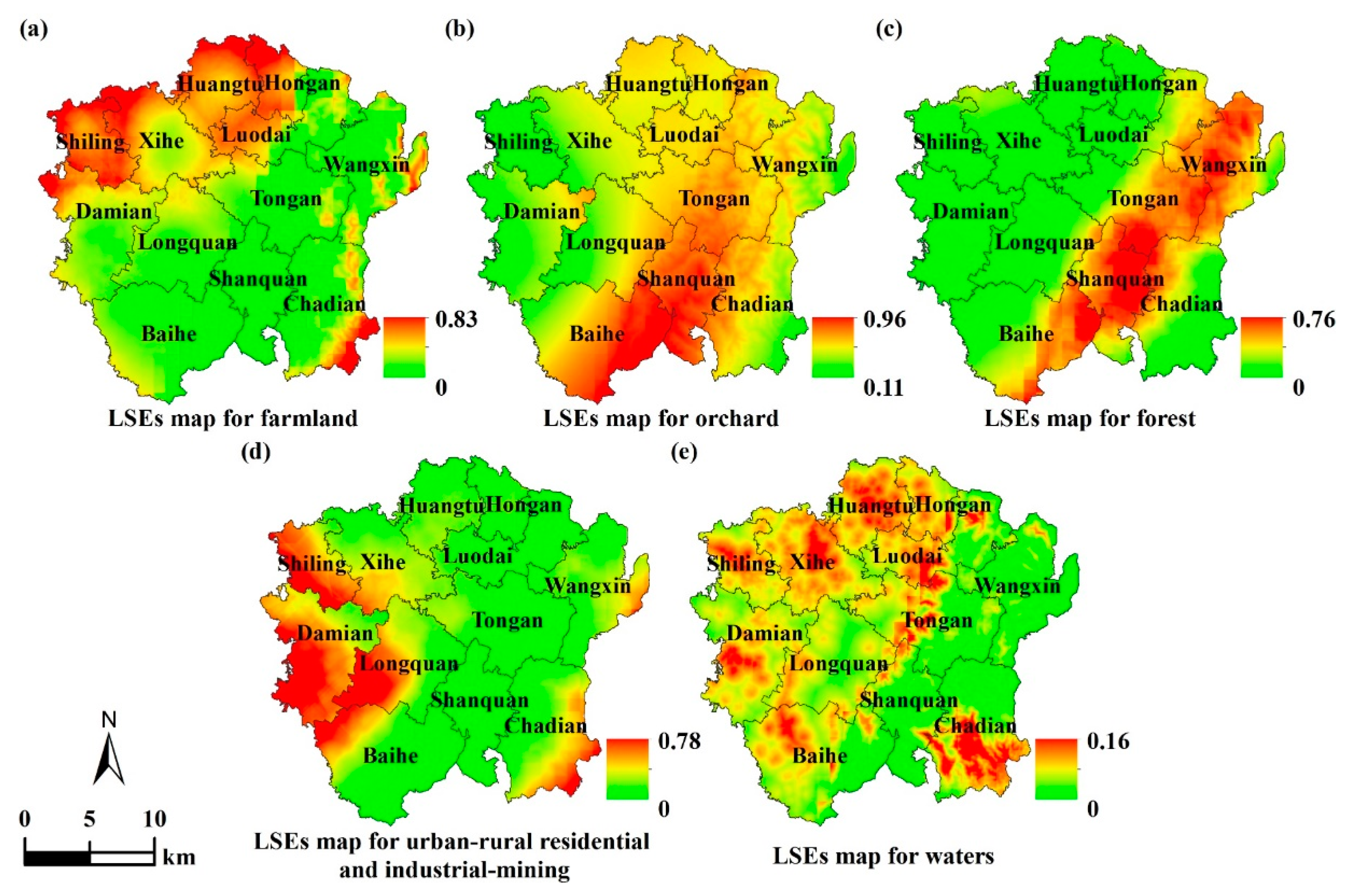
Among the BLR models for all the landscape types (Table 5), the predictive accuracies of the modeling and test data using the BLR model were 85.1% and 85.3% for farmland landscape, respectively, both accuracies were 65.6% for orchard landscape, 90.1% and 89.5% for forest landscape, 82.7% and 81.7% for urban-rural residential and industrial-mining landscape, and 97.2% and 97.6% for waters landscape. Thus, the predictive accuracy was high for each landscape type and the results predicted by the model were highly reliable. In addition, the ROC values obtained by the BLR model for each landscape type were all higher than 0.7 (Table 5). Therefore, the evaluation indicators selected for the regression equation had high explanatory power for the effects of landscape patterns, and thus these indicators were used for suitability evaluations of landscape patterns.
In addition, Figure 6 shows the spatial characteristics of the suitability evaluation results for each landscape type in the study area. The higher suitability areas for farmland were mainly distributed in the towns of Shiling, Huangtu, Hongan, Luodai, Xihe, and east of Wanxing, surrounding Longquan Lake in the town of Chadian. The higher suitability areas for orchard were mainly distributed in the towns of Shanquan and Tongan, east of Baihe, and west of Chadian and Wanxing. The higher suitability areas for forest were mainly distributed in the towns of Shanquan, Wanxing, and Baihe, east of Tongan, and west of Chadian. The higher suitability areas for urban-rural residential and industrial-mining were mainly distributed in the towns on plains in the study area, such as Shiling, Damian, Xihe, Longquan, and Baihe. The higher suitability areas for waters were mainly distributed in the towns on plains in the study area, such as Shiling, Xihe, Huangtu, Hongan, Luodai, Damian, Tongan, and Baihe, as well as Longquan Lake and its surrounding areas to the south of Chadian in the mountains in the study area. According to these characteristic distributions, there was some overlapping in the higher suitability areas for orchard and forest, where the overlapping distribution areas were distributed centrally to the east of Shanquan, Baihe, and Tongan, and to the west of Chadian.

3.2. Optimal Results Obtained by the LPQSO Model

Using the LPQSO model, we obtained the optimal areas for farmland, orchard, forest, urban-rural residential and industrial-mining, and waters under the economic development, ecological protection, and overall consideration scenarios in the target years of 2021 and 2028, as shown in Table 6. Compared with the area for each landscape type in the year 2014, the optimal areas for each landscape type under each scenario in the target year (Table 6) exhibited specific characteristics, as follows.
Under the economic development scenario, the areas for urban-rural residential and industrial-mining and farmland increased, whereas the area for orchard decreased, while the areas for forest and waters were unchanged. Moreover, the area for urban-rural residential and industrial-mining increased the most, whereas the area for orchard decreased the most. Thus, the scheme can achieve the maximum objective in terms of economic benefit because the economic benefit of urban-rural residential and industrial-mining is higher than that of orchard. Hence, the results obtained by the scheme agreed with the actual economic development scenario.
Under the ecological protection scenario, the areas for forest and farmland increased, whereas the area for orchard decreased, while the areas for urban-rural residential and industrial-mining and waters were unchanged. Moreover, the area for forest increased the most, whereas the area for orchard decreased the most. Thus, orchard was changed to forest by the scheme to achieve the maximum ecological security degree because the ecological security associated with forest is higher than that linked with orchard. Hence, the results obtained by the scheme agreed with the actual ecological protection scenario.
Under the overall consideration scenario, the areas for forest, urban-rural residential and industrial-mining, and farmland increased, whereas the area for orchard decreased, while the area for waters was unchanged. Moreover, the area for forest increased the most, followed by the area for urban-rural residential and industrial-mining, and the area for orchard decreased the most. Thus, orchard was changed to forest and urban-rural residential and industrial-mining, thereby significantly improving the maximum comprehensive benefit, including economic and ecological benefits, because the ecological security degree associated with forest and the economic benefit of urban-rural residential and industrial-mining are higher than those linked with orchard. Hence, the results obtained by the scheme agreed with the actual overall consideration scenario.

3.3. Optimal Results Obtained by the LPSLO Model

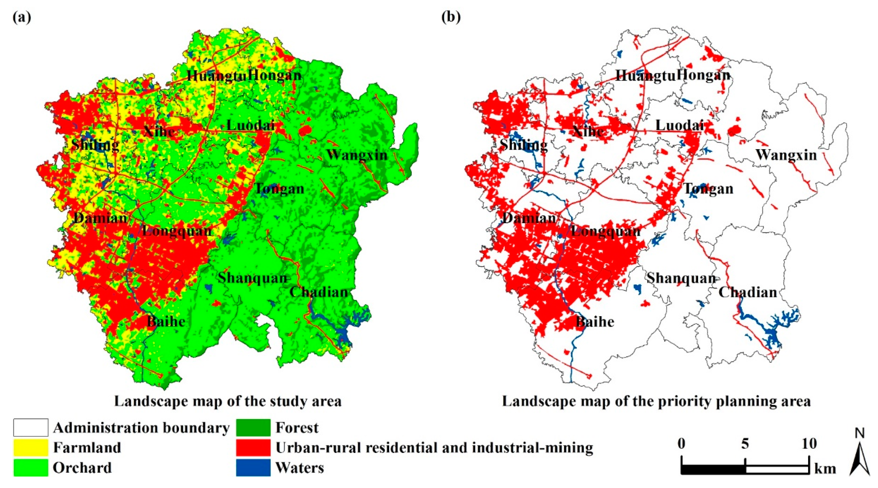
According to the basic data, such as the landscape map for the base year 2014 (Figure 2a), landscape maps of the priority planning areas (Figure 2b), spatial suitability evaluation maps for each landscape type (Figure 6), and quantitative structure optimization areas for each landscape under each scenario in the target year (Table 6), we obtained the landscape pattern spatial layout schemes for each scenario in the target years of 2021 and 2028 by using the LPSLO model and solution algorithm implemented in MATLAB, as shown in Table 7 and Figure 7. 
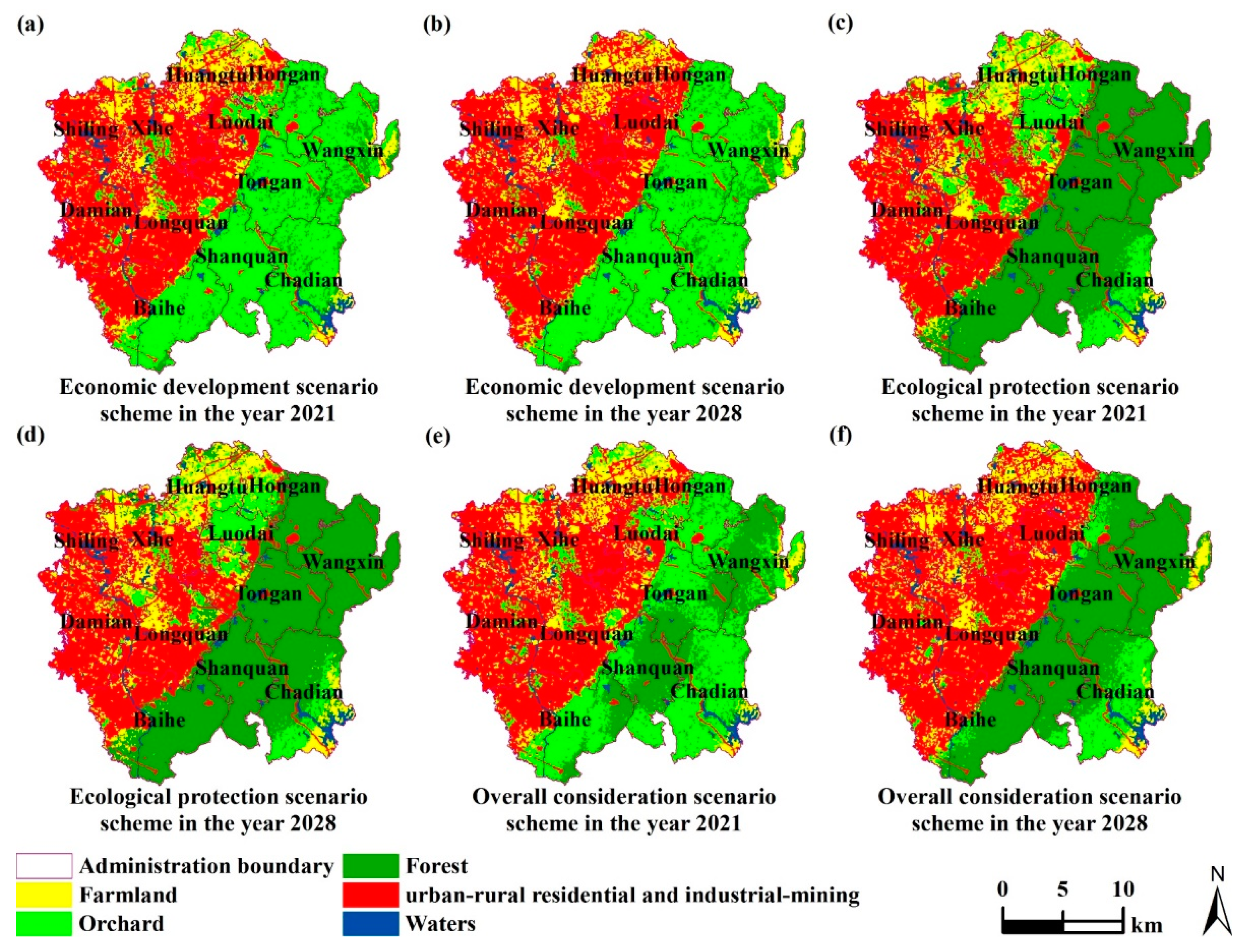
Figure 7 shows that the optimization results obtained for the landscape pattern spatial layout under each scenario in the target year had specific characteristics, as follows.
Under the economic development scenario, in the target year 2021, farmland was distributed throughout towns on the plains, including Huangtu, Hongan, and Xihe, as well as east of towns in mountainous areas such as Wanxing and Chadian; orchard was distributed in towns in mountainous areas, such as Shanquan, Chadian, and Wanxing, as well as east of Luodai, Tongan, and Baihe; forest was distributed in the towns of Wanxing and Chadian, as well as east of the towns of Luodai, Tongan, and Baihe; urban-rural residential and industrial-mining was distributed centrally in the towns of Shiling, Xihe, Damian, Longquan, Huangtu, and Hongan, and west of Luodai, Tongan, and Baihe; waters were mainly distributed in lakes in the mountainous region to the east of the study area, and in ponds and canals in the plains to the west of the study area. Compared with the landscape spatial layout under the economic development scenario in the target year of 2021, the areas covered by urban-rural residential and industrial-mining and farmland increased in the target year of 2028, whereas the area covered by orchard decreased.
Under the ecological protection scenario, in the target year of 2021, farmland was distributed throughout towns on the plains, including Huangtu, Hongan, Xihe, and Longquan, as well as the areas surrounding Longquan Lake in the town of Chadian in the mountainous region of the study area; orchard was distributed in towns on the plains such as Huangtu, Hongan, and Luodai, as well as southeast of Chadian in the mountainous region of the study area; forest covered the whole areas of the towns of Shanquan and Wanxing, as well as east of Baihe, Tongan, and Luodai, and northwest of Chadian; urban-rural residential and industrial-mining was distributed centrally in the towns of Shiling, Xihe, Damian, and Longquan, as well as west of the towns of Tongan and Baihe; while the characteristic distribution of the waters landscape spatial layout was similar to that under the economic development scenario. Compared with the landscape spatial layout under the ecological protection scenario in the target year of 2021, the areas covered by forest and farmland increased in the target year of 2028, whereas the area covered by orchard decreased.
Under the overall consideration scenario, in the target year 2021, farmland was distributed throughout the towns on the plain, including Huangtu, Hongan, and Xihe, as well as east of Wanxing and Chadian in the mountainous region of the study area; orchard was distributed mainly in the towns of Luodai and Chadian, as well as east of Tongan and Baihe, but less widely in the towns of Shanquan, Wanxing, Huangtu, Xihe, and Longquan; forest was distributed mainly to the east of Tongan and Baihe, and in the towns on the plains, such as Wanxing and Shanquan; urban-rural residential and industrial-mining was distributed mainly in the towns of Shiling, Xihe, Damian, and Longquan, and west of Tongan, Baihe, and Luodai, but less widely in the towns of Huangtu and Hongan; while the distribution characteristics of the landscape spatial layout for waters was similar to that under the economic development scenario as well as the ecological protection scenario. Compared with the landscape spatial layout under the overall consideration scenario in the target year of 2021, the area covered by forest increased in the target year of 2028 to cover the whole of the towns of Wanxing and Chadian, as well as east of the towns of Luodai, Tongan, and Baihe, and northwest of Chadian, whereas the area covered by orchard decreased greatly in the target year of 2028, where it was mainly distributed southeast of Chadian and on the piedmont to the east of Luodai.

4. Discussion

4.1. Analysis of the LPOA Model for Longquanyi

4.1.1. Accuracy of the Spatial Optimization Results

There were differences in the optimal areas obtained by LPSLO and LPQSO for each scenario in the target year (Table 5 and Table 6). The maximum error obtained after spatial optimization was for the forest area under the economic development scenario in the target year of 2028, where the relative error before and after optimization with the LPSLO model was 3.47%. The minimum error obtained after spatial optimization was for the urban-rural residential and industrial-mining area under the economic development scenario in the target year of 2028, where the relative error before and after optimization with the LPSLO model was 0.08%. Thus, the solutions obtained by the LPSLO model could not satisfy the equality constraints because of the effects of some particle elements during the flight process. Therefore, the solutions obtained by the model could not satisfy the equality constraints because the locations of particle elements corresponding to certain landscape types were replaced by particle elements corresponding to other landscape types during the flight process (i.e., the first particle element moved to a location while the second particle element moved to the same location occupied previously), thereby decreasing the previous landscape type area but increasing the subsequent landscape type area. According to the principles of the LPSLO model and the algorithm, the initial particles fully satisfy the equality constraints at initialization. However, the equality constraints are broken by some particles because the objective function values of some particles that break the equality constraints are higher than those of the initial particles. Thus, the landscape pattern spatial layout undergoes further optimization. Moreover, breaking the equality constraints in a specific error range may be a strategy for resolving the coupling problem between the objective functions for LPQSO and LPSLO. Thus, the LPSLO model can be used to optimize the landscape pattern spatial layout.
Furthermore, in order to validate the reliability and feasibility of the LPSLO model proposed in this study, we quantitatively assessed the accuracy of the landscape pattern simulation results using the widely employed confusion assessment method [46], where we compared the simulated and actual landscape pattern maps, and the accuracy was computed based on point-by-point comparisons using a confusion matrix. First, considering that Longquanyi District has been undergoing a period of rapid economic development and urbanization in the past ten years, we set the current landscape pattern status in the base year of 2014 as the actual landscape pattern for the economic development scenario. Next, according to the grid number for each landscape type in the current landscape pattern status in 2014, we obtained the simulated spatial allocation of the landscape pattern under the economic development scenario by using the LPSLO model with the parameters given above. Using ENVI 5.1, the confusion matrix shown in Table 8 was computed by comparing the simulated results obtained by the LPSLO model with the current landscape pattern status map in 2014 for each cell. The results showed that the overall accuracy of the simulated results was 84.98% and the Kappa coefficient was 0.7587, thereby indicating that the LPSLO model could simulate the landscape pattern spatial layout objectively and accurately. Therefore, it is feasible to employ this model to simulate the spatial allocation of future landscape patterns under each scenario based on the LPQSO model and LSE model, and thus the simulated results obtained were acceptable.

4.1.2. Rationality of the Spatial Optimization Results

In order to analyze the rationality of the spatial optimization results, we compared the characteristics of the current landscape pattern spatial status in the base year of 2014 with the landscape pattern optimization spatial layouts for the target years of 2021 and 2028, where the changes were analyzed according to the algorithm for the LPSLO model. As shown in Figure 2 and Figure 7, Table 6 and Table 7, the landscape pattern spatial optimization layout for each scenario in the target year exhibited specific characteristics, as follows.
Under the economic development scenario, the landscape pattern spatial layout obtained by the optimal schemes for the two periods indicated large increases in the urban-rural residential and industrial-mining areas but large decreases in orchard, while the forest and waters areas increased slightly and farmland decreased slightly. According to the algorithm in the LPSLO model, parts of some landscape types with lower suitability would be adjusted for other landscape types with higher suitability, while the optimized quantitative structure area for the former landscape type was decreased in the target years compared with the area of the corresponding landscape types in the base year, whereas the area for the latter landscape type in the target year was better than the area for the corresponding landscape types in the base year. Thus, the urban-rural residential and industrial-mining areas increased greatly compared with the corresponding area in the base year because the optimized quantitative structure areas in the target years were greater than the corresponding area in the base year. In addition, the orchard area decreased greatly because the optimized quantitative structure area was smaller in the target years than the corresponding area in the base year. However, the optimized quantitative structure areas for farmland in the target years were greater than those in the base year, and the optimized quantitative structure areas for forest and waters were the same as those in the base year, while the areas for farmland decreased slightly and the areas for forest and waters increased slightly. This was probably because the objective function value was improved by reducing the area of farmland and by increasing the areas for forest and waters according to the algorithm in the LPSLO model, as well as due to the error caused by particles colliding during the flight process.
Under the ecological protection scenario, the optimized landscape pattern spatial layouts obtained in the two periods indicated increases in the forest and urban-rural residential and industrial-mining areas, but decreases in the farmland and orchard areas, while the waters areas were unchanged. The optimized spatial areas for forest were increased compared with the corresponding area in the base year. This was mainly because the optimized quantitative structure areas in the target year were larger than the corresponding area in the base year, and thus other landscape types that were highly suitable for conversion into forest landscape were converted by the algorithm in the LPSLO model. Thus, the optimized spatial areas for orchard decreased because their optimized quantitative structure areas in the target year were smaller than the corresponding area in the base year, and thus the low suitability regions were converted into other landscape types by the algorithm in the LPSLO model. However, similar to the farmland, forest, and waters types under the economic development scenario, although the optimized quantitative structure areas for farmland were larger in the target years than the base year and the areas for urban-rural residential and industrial-mining were also the same in the target years as the base year, the optimized spatial areas for farmland decreased and the areas for urban-rural residential and industrial-mining increased.
Under the overall consideration scenario, the optimized landscape pattern spatial layouts in the two periods indicated that the areas for urban-rural residential and industrial-mining and forest increased greatly, whereas the areas for orchard and farmland decreased, while the waters areas were unchanged, in the same manner as the ecological protection scenario. Given that the human demand for landscape resources is unlimited, game selection among the various landscape types was necessary during the spatial optimization process because of the finite amount of land to sustain landscape resources. Therefore, the weights for the urban-rural residential and industrial-mining and forest types shown in Table 4 were larger than those for other landscape types, and thus they were preferentially increased in the specified area. Furthermore, waters had a low weight but there was little spatial change in the areas for water areas because a protection strategy for water resources was considered in the LPSLO model (Figure 2). In addition, the difference between the weights was slight for orchard and farmland, but the orchard type decreased greatly, whereas the farmland type only decreased slightly. This was mainly because the high suitability areas for orchard overlapped with those for forest in the study area (Figure 6), and thus orchard was favored less by the game selection where forest had a higher weight than orchard, so the spatial expansion of orchard decreased greatly.

4.1.3. Comparative Analysis of the LPOA Scheme Under Each Scenario

In order to conduct comparative analyses of the LPOA schemes under each scenario, we analyzed the feasibility of the landscape pattern spatial allocation scheme for each scenario in the target years by considering the actual status of socioeconomic development and ecological construction. The Chinese economy has slowed down, but the overall economy and population of Longquanyi District will continue to increase in the future because this area is located in a special location for economic growth, i.e., a suburban area of Chengdu City, and it is the location of the high-end manufacturing industry in Sichuan province. Population growth will inevitably lead to increases in the demand for land for residential and public service uses as well as for economic development, which will increase the demand for industrial land and ancillary land. Hence, the potential growth of urban-rural residential and industrial-mining areas will be very high in this area in the future. Substantial increases in urban-rural residential and industrial-mining areas will decrease the availability of other landscape resources, including farmland, orchard, forest, and waters landscape types because of the finite availability of land resources. However, the growth of forest and waters landscape types has greater ecological benefits and Longquanyi is a National Ecological Demonstration Zone, so a decrease in ecological construction efforts is unlikely, and thus potential decreases in the farmland and orchard landscape types are very likely in the future. Under the economic development scenario for landscape patterns, we found that the urban-rural residential and industrial-mining area increased greatly whereas the orchard area decreased considerably in order to achieve the maximum economic benefit. However, the areas of the forest, waters, and farmland landscape types changed little, especially forest, which has higher ecological value and it increased slightly. This is inconsistent with the actual situation because the growth of forest in this area has high potential. Thus, the feasibility of the schemes obtained under this scenario may be lower in the future. Under the ecological protection scenario for landscape patterns, the area of forest increased greatly when emphasizing the maximum ecological security level. However, in this scheme, there was not an adequate supply of urban-rural residential and industrial-mining land, which maintains steady economic growth, and this is inconsistent with the actual situation where a substantial expansion of land allocated to urban-rural residential and industrial-mining is very likely. Thus, the feasibility of the scheme obtained under this scenario is also less likely in the future. Under the overall consideration scenario for landscape patterns, the scheme considered the supply of land resources required to maintain economic growth as well as the ecological resources required to improve the quality of the environment, so there were adequate allocations to the urban-rural residential and industrial-mining landscape type to maintain economic growth and to the forest landscape type to preserve ecological security. This scheme agrees with the likely changes in the regional landscape as well as providing appropriate allocations to meet the actual needs of economic development and ecological construction in the study area. Thus, the scheme obtained under this scenario is the most likely compared with the other two schemes and it is the optimal scheme for determining the future landscape pattern spatial layout in the study area.

4.2. Discussion of the Potential Usefulness of the LPOA Model

4.2.1. Useful Results obtained from the Application of the LPOA Model

Three useful results were obtained from the application of the LPOA model, i.e., a planning concept for balancing economic and ecological benefits, a planning strategy that considers both quantitative structure optimization and spatial layout optimization, and a planning strategy that closely connects the theoretical model with the actual region, and these results provide a useful reference for formulating related spatial planning activities, including landscape pattern planning, land use planning, and urban planning in other regions.
First, the conflict between economic development and ecological protection has become the principal contradiction that affects sustainable development in human society. During the modernization process throughout the world, many disasters have been caused by ignoring ecological protection while focusing on economic construction, such as nuclear pollution, air pollution, ocean pollution, rainforest felling, and industrial mining. However, the desire for a better life is the tireless pursuit of humanity. We cannot stop economic development to protect the ecological environment or seek economic development at the expense of the environment. Thus, balancing the conflict between the needs of economic development and ecological protection is a major problem which must be solved urgently to allow the sustainable development of human society. The LPOA model optimization results confirmed that LPOA, by balancing economic and ecological benefits, is an effective approach for mitigating conflicts between economic development and ecological protection from the perspective of spatial planning. This planning concept can provide a useful reference for other regions when conducting landscape pattern planning, land use planning, urban planning, and other related spatial planning processes.
Second, in the past, when we formulated spatial planning processes such as land use planning and urban planning, we attached great importance to planning and forecasting the resource quantity in the target year, whereas we often ignored the rational spatial allocation of resources, thereby making some plans difficult to implement because spatial optimization allocation planning was ignored. The LPOA model achieves a successful planning strategy by effectively coupling the landscape quantity structure with the spatial layout during the LPOA process. Other regions can employ this planning strategy to guide the preparation of landscape pattern planning, land use planning, urban planning, and other related forms of spatial planning.
Third, many spatial optimization models were mentioned above, but most are difficult to apply directly for practical planning. This is mainly because some optimization models fail to consider macrofactors, including social, economic, policy, system, and other factors, and thus the optimization results are far from reality and difficult to implement. During the LPOA process, the LPOA model first formulates large urban built-up areas and waters as priority planning areas, before applying the optimization model to spatially optimize the allocation of the landscape pattern in other areas, thereby allowing the effective combination of macrofactors and theoretical models. This approach is universal because when formulating similar types of spatial planning in other regions, specified unadjusted areas (e.g., ecological protection and basic farmland protection zones) can be planned as priority planning zones and the other areas can be subjected to spatial layout optimization allocation using the optimization model, thereby ensuring a close connection between the theoretical model and the reality in the region.

4.2.2. Beneficial Contributions of the LPOA Model

The LPOA model addresses three problems related to the current spatial optimization decision-making methods, such as neglecting the coupling between quantitative structure optimization and spatial layout optimization, ignoring the macrofactors that affect landscape patterns when optimizing modeling, and initializing particles without considering the suitability of the landscape. Our proposed LPOA model is beneficial because it can complement the simulation of spatial optimization allocation processes, such as LPOA, land use spatial allocation, urban space optimization allocation.
First, the key to establishing the LPOA model is integrating the landscape optimal area, landscape suitability, and macrofactors (e.g., social, economic, policy, and system factors) in order to conduct the LPOA to maximize the landscape benefits. We established a new LPOA model for optimizing the allocation of the landscape spatial pattern by integrating the landscape optimal area, landscape suitability, and macrofactors that influence landscape patterns in order to maximize the economic, ecological, and comprehensive benefits of landscape patterns. The optimal landscape areas in various landscape types are optimized with the LPQSO model based on NP. The suitability of each landscape type is then calculated with the LSE model based on BLR. The macrofactors that affect landscape patterns are combined with the LPOA models by setting model constraint conditions and priority planning areas. A PSO evolutionary algorithm is then embedded into the LPSLO model in order to integrate the results obtained by the LPQSO and LSEs, thereby establishing an LPOA model and algorithm to address the problems caused by ignoring the coupling between quantitative structure optimization and spatial layout optimization, the macrofactors that affect landscape patterns when optimizing modeling, and the suitability of landscape types, as found in previous studies.
Second, based on raster data, the focus when optimizing the landscape pattern spatial layout using PSO is how to use the positions of particle elements to simulate the spatial positions of cells for landscape type raster graphics, and establishing the spatial mapping of the relationships between landscape type raster graphics and particles. We assume that the matrix denotes the landscape type raster map and the matrix element value denotes the pixel attribute value of the landscape type raster map. The matrix is abstracted as a particle that corresponds to a landscape pattern spatial layout scheme. The matrix element value is abstracted as particle element that corresponds to a landscape type code. According to the principle of the PSO algorithm, we can program using the powerful matrix operation capability in MATLAB software to simulate the particle flight process to search for the best scheme for the landscape pattern spatial layout, i.e., a matrix element value moves from one location to another by adjusting its row and column numbers to form a new matrix (a new landscape pattern spatial layout scheme). Thus, the LPSLO is obtained successfully when the new matrix corresponding to the landscape pattern spatial layout achieves the maximum optimization objective. The type and number of the particle element (landscape type code) comprising the particle (landscape pattern spatial layout scheme) will never change in terms of its spatial position. Therefore, according to the landscape suitability and landscape type conversion rules, we generate an initial particle with an element number equal to the grid number for the optimal area of the corresponding landscape type based on the landscape type raster map in the base year, which effectively combines landscape pattern quantity structure optimization and spatial layout optimization, as well as skillfully integrating the landscape suitability evaluation results during the optimization of the landscape spatial layout. Therefore, this approach successfully overcomes the problem of neglecting the coupling between quantitative structure optimization and spatial layout optimization for the landscape pattern, as well as addressing the problem of ignoring the landscape suitability when initializing particles.
Third, during the establishment of the spatial mapping relationship between the landscape type raster graphics and particles, we first set the code value of landscape type in the priority planning area as negative values (e.g., setting the code value for urban-rural residential and industrial-mining as −4 or setting the code value for waters as −5), and encode the landscape type code values in other areas as positive values (e.g., setting the code values for farmland, orchard, forest, urban-rural residential and industrial-mining, and waters as 1, 2, 3, 4, and 5, respectively). We then define the elements with codes that have positive values as the valid elements and store them as vector quantity data structures denoting a particle, whereas we define the elements with codes that have negative and null values as invalid elements that do not map to particles, i.e., the invalid elements will not participate in the optimization allocation for the spatial locations. Thus, after each iterative computation of the particles, we amalgamate the landscape pattern spatial layout corresponding to the invalid elements in the priority planning area with the landscape pattern spatial layout searched for by the flight of the particles, and then calculate the particle fitness based on the merged spatial layout to obtain the optimal scheme of LPOA for the entire area. Therefore, this approach allows the effective combination of the spatial optimization model and macroscopic factors, such as society, economy, policy, and system factors, as well as successfully addressing the problem of coupling macroscopic factors that affect the landscape pattern with the spatial optimization model.

5. Conclusions

In this study, we proposed a new composite model called the LPOA model for optimizing the spatial allocation of a landscape pattern, which aims to solve a set of optimal problems in LPOA, such as neglecting the coupling between quantitative structure optimization and spatial layout optimization, ignoring the macrofactors that affects landscape patterns during optimization modeling, and initializing particles without considering the suitability of the landscape. The LPOA model mainly comprises LSEs, LPQSO, and LPSLO, where it successfully integrates BLR and NP with PSO, thereby overcoming the problem of optimizing either the quantitative structure or the spatial layout of the landscape pattern, as found in previous studies, as well as addressing the problem of ignoring the landscape suitability and macrofactors that influence the landscape pattern during the LPOA process. The model proposed in this study is a beneficial and useful complement to methods for simulating the spatial optimization allocation, such as LPOA, land use spatial allocation, and urban space optimization allocation, thereby providing a useful reference for formulating related spatial planning processes, including landscape pattern planning, land use planning, and urban planning, in other regions.
We employed the LPOA model to optimize the landscape pattern for the target years of 2021 and 2028 in Longquanyi District. We found that the LPOA model could simultaneously optimize the quantitative structure and spatial landscape pattern, as well as effectively integrating the landscape suitability and relevant factors that influence landscape patterns, such as social, economic, policy, and system factors. Moreover, the LPOA model could optimize the landscape pattern in terms of its quantitative structure, spatial layout, and benefits, where we established optimized landscape pattern schemes under economic development, ecological protection, and overall consideration scenarios. The model significantly improved the overall economical, ecological, and comprehensive benefits of the landscape pattern. In addition, we assessed and analyzed the accuracy and rationality of the spatial optimization results, where we found that the overall accuracy of the spatial optimal results was 84.98% with a Kappa coefficient of 0.7587. This indicates that performance of the LPSLO model was good and the application of this model can satisfy the demands for LPOA under multiple constraints. Furthermore, the results obtained by the simulated scheme were consistent with the actual situation. The proposed model can provide support and a scientific basis for regional landscape pattern planning, land use planning, urban planning, and other related spatial planning.
LPOA is a complex and multiobjective decision-making process. In this study, we present a new LPOA model that integrates LSE and LPQSO models with an LPSLO model based on the grid units in a landscape type raster map. Our results demonstrated that this model can achieve LPOA by simultaneously combining the quantitative structure optimized using the LPQSO model, the spatial layout optimized using the LPSLO model, the landscape suitability obtained using the LSE model, as well as the macrofactors that affect landscape patterns, including social, economic, policy, and system factors. However, the number of calculations required by this model and the runtime of the algorithm increase with the resolution of the raster images or the size of the study area, so it is necessary to select a raster map with an appropriate resolution according to the study area size and research scale before conducting spatial optimal decision making with this model. Furthermore, by considering the coupling of the objective functions for both the LPQSO and LPSLO models, as well as the efficiency of the algorithm, the proposed model does not include particle collision constraints. The relative error in the calculation results is acceptable for macroplanning in terms of regional landscape security patterns. Nevertheless, it is necessary to specify particle collision constraints after resolving the coupling problem between the objective functions for LPQSO and LPSLO, as well as improving the efficiency of the algorithm for the LPOA model when conducting detailed planning and design for landscape patterns and other related spatial planning.

Author Contributions

Conceptualization, D.O. and J.X.; methodology, D.O.; software, D.O.; validation, D.O., X.Y., X.G. and J.Y.; formal analysis, D.O., X.Y., X.G. and Z.H.; investigation, D.O., W.C. and X.Y.; resources, D.O., J.X., X.G. and C.W.; data curation, D.O., X.Y., Q.L. and Z.H.; writing the original draft preparation, D.O.; writing the review and editing, D.O. and W.C.; visualization, D.O., X.Y., Q.L. and J.Y.; supervision, D.O. and C.W.; project administration, D.O. and J.X.; funding acquisition, D.O., J.X., X.G. and C.W.

Funding

This research was funded by the Double Support Program Project of Discipline Construction of Sichuan Agricultural University of China (No. 2018), Cultivating Funds of Academic and Technical Leaders of Sichuan Province of China (No. 2014), Science and Technology Program Project of Sichuan Province of China (Nos. 2013GZ0024, 2017GZ0325), and National Key Technology Research and Development Program of the Ministry of Science and Technology of China (No. 2008BAD98B05).

Acknowledgments

The authors would like to thank the anonymous reviewers for their valuable comments, which helped us improve the original manuscript.

Conflicts of Interest

The authors have no conflicts of interest to declare.

References

  1. Deng, X.; Huang, J.; Rozelle, S.; Zhang, J.; Li, Z. Impact of urbanization on cultivated land changes in China. Land Use Policy 2015, 45, 1–7. [Google Scholar] [CrossRef]
  2. Chen, W.; Carsjens, G.; Zhao, L.; Li, H. A spatial optimization model for sustainable land use at regional level in China: A case study for Poyang Lake region. Sustainability 2015, 7, 35–55. [Google Scholar] [CrossRef]
  3. Liu, Y.; Huang, X.; Yang, H.; Zhong, T. Environmental effects of land-use/cover change caused by urbanization and policies in Southwest China Karst area—A case study of Guiyang. Habitat Int. 2014, 44, 339–348. [Google Scholar] [CrossRef]
  4. Bawa, K.S.; Koh, L.P.; Lee, T.M.; Liu, J.; Ramakrishnan, P.S.; Douglas, W.Y.; Zhang, Y.P.; Raven, P.H. China, India, and the environment. Science 2010, 327, 1457–1459. [Google Scholar] [CrossRef] [PubMed]
  5. Li, T.; Shilling, F.; Thorne, J.; Li, F.; Schott, H.; Boynton, R.; Berry, A.M. Fragmentation of China’s landscape by roads and urban areas. Landsc. Ecol. 2010, 25, 839–853. [Google Scholar] [CrossRef]
  6. Liu, Y.; Liu, D.; Liu, Y.; He, J.; Jiao, L.; Chen, Y.; Hong, X. Rural land use spatial allocation in the semiarid loess hilly area in China: Using a Particle Swarm Optimization model equipped with multi-objective optimization techniques. Sci. China Earth Sci. 2012, 55, 1166–1177. [Google Scholar] [CrossRef]
  7. Yang, L.; Sun, X.; Peng, L.; Shao, J.; Chi, T. An improved artificial bee colony algorithm for optimal land-use allocation. Int. J. Geogr. Inf. Sci. 2015, 29, 1470–1489. [Google Scholar] [CrossRef]
  8. Tong, H.; Shi, P.; Bao, S.; Zhang, X.; Nie, X. Optimization of urban land development spatial allocation based on ecology-economy comparative advantage perspective. J. Urban Plan. Dev 2018, 144, 05018006. [Google Scholar] [CrossRef]
  9. Li, F.; Gong, Y.; Cai, L.; Sun, C.; Chen, Y.; Liu, Y.; Jiang, P. Sustainable land-use allocation: A multiobjective particle swarm optimization model and application in Changzhou, China. J. Urban Plan. Dev. 2018, 144, 04018010. [Google Scholar] [CrossRef]
  10. Yue, D.; Wang, J.; Liu, Y.; Zhang, X.; Li, H.; Wang, J. Ecologically based landscape pattern optimization in northwest of Beijing. J. Geogr. Sci. 2009, 19, 359–372. [Google Scholar] [CrossRef]
  11. Jiang, M.; Chen, H.; Chen, Q.; Wu, H. Study of landscape patterns of variation and optimization based on nonpoint source pollution control in an estuary. Mar. Pollut. Bull. 2014, 87, 88–97. [Google Scholar] [CrossRef]
  12. Zhang, J.; Fu, M.; Zhang, Z.; Tao, J.; Fu, W. A trade-off approach of optimal land allocation between socio-economic development and ecological stability. Ecol. Model. 2014, 272, 175–187. [Google Scholar] [CrossRef]
  13. Tang, L.; Wang, H.; Wang, L.; Qiu, Q. Landscape pattern optimization for Xianghe Segment of China’s Grand Canal. Int. J. Sustain. Dev. World Ecol. 2015, 23, 305–311. [Google Scholar] [CrossRef]
  14. Liu, Y.; Peng, J.; Jiao, L.; Liu, Y. PSOLA: A heuristic land-use allocation model using patch-level operations and knowledge-informed rules. PLoS ONE 2016, 11, e0157728. [Google Scholar] [CrossRef] [PubMed]
  15. Masoumi, Z.; Maleki, J.; Mesgari, M.S.; Mansourian, A. Using an evolutionary algorithm in multiobjective geographic analysis for land use allocation and decision supporting. Geogr. Anal. 2017, 49, 58–83. [Google Scholar] [CrossRef]
  16. Sharmin, N.; Haque, A.; Islam, M.M. Generating Alternative land-use allocation for mixed use areas: Multi-objective optimization approach. Geogr. Anal. 2018, 25, 62–73. [Google Scholar] [CrossRef]
  17. Liu, X.; Li, X.; Shi, X.; Huang, K.; Liu, Y. A multi-type ant colony optimization (MACO) method for optimal land use allocation in large areas. Int. J. Geogr. Inf. Sci. 2012, 26, 1325–1343. [Google Scholar] [CrossRef]
  18. Kucukmehmetoglu, M.; Geymen, A. Optimization models for urban land readjustment practices in Turkey. Habitat Int. 2016, 53, 517–533. [Google Scholar] [CrossRef]
  19. Mohammadi, M.; Nastaran, M.; Sahebgharani, A. Development, application, and comparison of hybrid meta-heuristics for urban land-use allocation optimization: Tabu search, genetic, GRASP, and simulated annealing algorithms. Comput. Environ. Urban Syst. 2016, 60, 23–36. [Google Scholar] [CrossRef]
  20. Türk, E.; Zwick, P.D. Optimization of land use decisions using binary integer programming: The case of Hillsborough County, Florida, USA. J. Environ. Manag. 2019, 235, 240–249. [Google Scholar] [CrossRef]
  21. Li, X.; Ma, X. An uncertain programming model for land use structure optimization to promote effectiveness of land use planning. Chin. Geogr. Sci. 2017, 27, 974–988. [Google Scholar] [CrossRef]
  22. Shen, Q.; Chen, Q.; Tang, B.; Yeung, S.; Hu, Y.; Cheung, G. A system dynamics model for the sustainable land use planning and development. Habitat Int. 2009, 33, 15–25. [Google Scholar] [CrossRef]
  23. Ma, X.; Zhao, X. Land use allocation based on a multioObjective artificial immune optimization model: An application in Anlu County, China. Sustainability 2015, 7, 15632–15651. [Google Scholar] [CrossRef]
  24. Santé-Riveira, I.; Crecente-Maseda, R.; Miranda-Barrós, D. GIS-based planning support system for rural land-use allocation. Comput. Electron. Agric. 2008, 63, 257–273. [Google Scholar] [CrossRef]
  25. Liu, X.; Ou, J.; Li, X.; Ai, B. Combining system dynamics and hybrid particle swarm optimization for land use allocation. Ecol. Model. 2013, 257, 11–24. [Google Scholar] [CrossRef]
  26. Feng, Y. Modeling dynamic urban land-use change with geographical cellular automata and generalized pattern search-optimized rules. Int. J. Geogr. Inf. Sci. 2017, 31, 1198–1219. [Google Scholar]
  27. Liang, X.; Liu, X.; Li, D.; Zhao, H.; Chen, G. Urban growth simulation by incorporating planning policies into a CA-based future land-use simulation model. Int. J. Geogr. Inf. Sci. 2018, 32, 2294–2316. [Google Scholar] [CrossRef]
  28. Zhou, R.; Zhang, H.; Ye, X.Y.; Wang, X.J.; Su, H.L. The delimitation of urban growth boundaries using the CLUE-S Land-Use Change Model: Study on Xinzhuang Town, Changshu City, China. Sustainability 2016, 8, 1182. [Google Scholar] [CrossRef]
  29. Kucsicsa, G.; Popovici, E.A.; Bălteanu, D.; Grigorescu, I.; Dumitraşcu, M.; Mitrică, B. Future land use/cover changes in Romania: Regional simulations based on CLUE-S model and CORINE land cover database. Landsc. Ecol. Eng. 2019, 15, 75–90. [Google Scholar] [CrossRef]
  30. Bakker, M.M.; Alam, S.J.; van Dijk, J.; Rounsevell, M.D. Land-use change arising from rural land exchange: An agent-based simulation mode. Landsc. Ecol. 2015, 30, 273–286. [Google Scholar] [CrossRef]
  31. Zagaria, C.; Schulp, C.J.; Kizos, T.; Gounaridis, D.; Verburg, P.H. Cultural landscapes and behavioral transformations: An agent-based model for the simulation and discussion of alternative landscape futures in East Lesvos, Greece. Land Use Policy 2017, 65, 26–44. [Google Scholar] [CrossRef]
  32. Bryan, B.A.; Crossman, N.D.; King, D.; Meyer, W.S. Landscape futures analysis: Assessing the impacts of environmental targets under alternative spatial policy options and future scenarios. Environ. Model. Softw. 2011, 26, 83–91. [Google Scholar] [CrossRef]
  33. Han, H.; Yang, C.; Song, J. Scenario simulation and the prediction of land use and land cover change in Beijing, China. Sustainability 2015, 7, 4260–4279. [Google Scholar] [CrossRef]
  34. Liu, X.; Liang, X.; Li, X.; Xu, X.; Ou, J.; Chen, Y.; Li, S.; Wang, S.; Pei, F. A future land use simulation model (FLUS) for simulating multiple land use scenarios by coupling human and natural effects. Landsc. Urban Plan. 2017, 168, 94–116. [Google Scholar] [CrossRef]
  35. Keshtkar, H.; Voigt, W. A spatiotemporal analysis of landscape change using an integrated Markov chain and cellular automata models. Model. Earth Syst. Environ. 2016, 2, 10. [Google Scholar] [CrossRef]
  36. Tian, G.; Ma, B.; Xu, X.; Liu, X.; Xu, L.; Liu, X.; Xiao, L.; Kong, L. Simulation of urban expansion and encroachment using cellular automata and multi-agent system model—A case study of Tianjin metropolitan region, China. Ecol. Indic. 2016, 70, 439–450. [Google Scholar] [CrossRef]
  37. Islam, K.; Rahman, M.F.; Jashimuddin, M. Modeling land use change using Cellular Automata and Artificial Neural Network: The case of Chunati Wildlife Sanctuary, Bangladesh. Ecol. Indic. 2018, 88, 439–453. [Google Scholar] [CrossRef]
  38. Liu, Y.; Tang, W.; He, J.; Liu, Y.; Ai, T.; Liu, D. A land-use spatial optimization model based on genetic optimization and game theory. Comput. Environ. Urban Syst. 2015, 49, 1–14. [Google Scholar] [CrossRef]
  39. Li, X.; Ma, X. An improved simulated annealing algorithm for interactive multi-objective land resource spatial allocation. Ecol. Complex. 2018, 36, 184–195. [Google Scholar] [CrossRef]
  40. Ma, S.; He, J.; Liu, F.; Yu, Y. Land-use spatial optimization based on PSO algorithm. Geo-Spat. Inf. Sci. 2011, 14, 54–61. [Google Scholar] [CrossRef]
  41. Huang, K.; Liu, X.; Li, X.; Liang, J.; He, S. An improved artificial immune system for seeking the Pareto front of land-use allocation problem in large areas. Int. J. Geogr. Inf. Sci. 2013, 27, 922–946. [Google Scholar] [CrossRef]
  42. Yang, L.; Zhu, A.; Shao, J.; Chi, T. A knowledge-informed and pareto-based artificial bee colony optimization algorithm for multi-objective land-use allocation. ISPRS Int. J. Geogr. Inf. Sci. 2018, 7, 63. [Google Scholar] [CrossRef]
  43. Masoomi, Z.; Mesgari, M.S.; Hamrah, M. Allocation of urban land uses by multi-objective particle swarm optimization algorithm. Int. J. Geogr. Inf. Sci. 2013, 27, 542–566. [Google Scholar] [CrossRef]
  44. Li, X. Emergence of bottom-up models as a tool for landscape simulation and planning. Landsc. Urban Plan. 2011, 100, 393–395. [Google Scholar] [CrossRef]
  45. Liu, Y.; Yuan, M.; He, J.; Liu, Y. Regional land-use allocation with a spatially explicit genetic algorithm. Landsc. Ecol. Eng. 2015, 11, 209–219. [Google Scholar] [CrossRef]
  46. Wang, S.; Wang, X.; Zhang, H. Simulation on optimized allocation of land resource based on DE-CA model. Ecol. Model. 2015, 314, 135–144. [Google Scholar] [CrossRef]
  47. Zhang, H.; Zeng, Y.; Jin, X.; Shu, B.; Zhou, Y.; Yang, X. Simulating multi-objective land use optimization allocation using Multi-agent system: A case study in Changsha, China. Ecol. Model. 2016, 320, 334–347. [Google Scholar] [CrossRef]
  48. Heydari, M.; Honarbakhsh, A.; Pajoohesh, M.; Zangiabadi, M. Land use optimization using the fuzzy mathematical-spatial approach: A case study of Chelgerd watershed, Iran. J. Environ. Eng. Landsc. Manag. 2018, 26, 75–87. [Google Scholar] [CrossRef]
  49. Wang, Q.; Liu, R.; Men, C.; Guo, L. Application of genetic algorithm to land use optimization for nonpoint source pollution control based on CLUE-S and SWAT. J. Hydrol. 2018, 560, 86–96. [Google Scholar] [CrossRef]
  50. Christodoulou, M.; Nakos, G. An approach to comprehensive land use planning. J. Environ. Manag. 1990, 31, 39–46. [Google Scholar] [CrossRef]
  51. Carsjens, G.J.; Van Knaap, W.D. Strategic land-use allocation: Dealing with spatial relationships and fragmentation of agriculture. Landsc. Urban Plan. 2002, 58, 171–179. [Google Scholar] [CrossRef]
  52. Özcan, Z.; Kentel, E.; Alp, E. Determination of unit nutrient loads for different land uses in wet periods through modelling and optimization for a semi-arid region. J. Hydrol. 2016, 540, 40–49. [Google Scholar] [CrossRef]
  53. Aljanabi, A.; Mays, L.; Fox, P. Optimization model for agricultural reclaimed water allocation using mixed-integer nonlinear programming. Water 2018, 10, 1291. [Google Scholar] [CrossRef]
  54. Grové, B. Improved Water Allocation under Limited Water Supplies Using Integrated Soil-Moisture Balance Calculations and Nonlinear Programming. Water Resour. Manag. 2019, 33, 423–437. [Google Scholar] [CrossRef]
  55. Van den Berg, F.; Engelbrecht, A.P. A study of particle swarm optimization particle trajectories. Inf. Sci. 2006, 176, 937–971. [Google Scholar] [CrossRef]
  56. Wang, S.; Watada, J. A hybrid modified PSO approach to Var-based facility location problems with variable capacity in fuzzy random uncertainty. Inf. Sci. 2012, 192, 3–18. [Google Scholar] [CrossRef]
  57. Hu, F.; Xu, W.; Li, X. A modified particle swarm optimization algorithm for optimal allocation of earthquake emergency shelters. Int. J. Geogr. Inf. Sci. 2012, 26, 1643–1666. [Google Scholar] [CrossRef]
  58. Chatterjee, S.; Sarkar, S.; Hore, S.; Dey, N.; Ashour, A.S.; Balas, V.E. Particle swarm optimization trained neural network for structural failure prediction of multistoried RC buildings. Neural Comput. Appl. 2017, 28, 2005–2016. [Google Scholar] [CrossRef]
  59. Xue, B.; Zhang, M.; Browne, W.N. Particle swarm optimization for feature selection in classification: A multi-objective approach. IEEE Trans. Cybern. 2013, 43, 1656–1671. [Google Scholar] [CrossRef]
  60. Zhang, M.; Ma, J.; Gong, M. Unsupervised hyperspectral band selection by fuzzy clustering with particle swarm optimization. IEEE Geosci. Remote Sens. Lett. 2017, 14, 773–777. [Google Scholar] [CrossRef]
  61. Abdel-Basset, M.; Fakhry, A.E.; El-Henawy, I.; Qiu, T.; Sangaiah, A.K. Feature and intensity based medical image registration using particle swarm optimization. J. Med. Syst. 2017, 41, 197. [Google Scholar] [CrossRef] [PubMed]
  62. Boeringer, D.W.; Werner, D.H. Particle swarm optimization versus genetic algorithms for phased array synthesis. IEEE Trans. Antennas Propag. 2004, 52, 771–779. [Google Scholar] [CrossRef]
  63. Ou, D.; Xia, J.; Zhang, L.; Zhao, Z.; Ou, X. The application of RS and GIS technology in meso-scale landscape classification and cartography: A case study in Longquanyi District of Chengdu. Chin. J. Ecol. 2015, 34, 2971–2982. (In Chinese) [Google Scholar]
  64. Pontius, R.G., Jr.; Schneider, L.C. Land-cover change model validation by an ROC method for the Ipswich watershed, Massachusetts, USA. Agric. Ecosyst. Environ. 2001, 85, 239–248. [Google Scholar] [CrossRef]
  65. Xie, G.; Lu, C.; Leng, Y.; Zheng, D.; Li, S. Ecological assets valuation of the Tibetan Plateau. J. Nat. Resour. 2003, 18, 189–196. (In Chinese) [Google Scholar]
  66. Eberhart, R.C.; Kennedy, J. A new optimizer using particle swarm theory. In Proceedings of the Sixth International Symposium on Micromachine and Human Science, Nagoya, Japan, 4–6 October 1995; pp. 39–43. [Google Scholar]
  67. Chapman, S.J. MATLAB Programming for Engineers, 4th ed.; Thomson Learning: Toronto, ON, Canada, 2008; pp. 2–19, 327–340. [Google Scholar]
  68. Eberhart, R.C.; Shi, Y. Particle swarm optimization: Developments, applications and resources. In Proceedings of the 2001 Congress on Evolutionary Computation, Seoul, Korea, 27–30 May 2001; pp. 81–86. [Google Scholar]
  69. Zhang, P.; Liu, Y.; Pan, Y.; Yu, Z. Land use pattern optimization based on CLUE-S and SWAT models for agricultural nonpoint source pollution control. Math. Comput. Model. 2013, 58, 588–595. [Google Scholar] [CrossRef]
  70. Batisani, N.; Yarnal, B. Uncertainty awareness in urban sprawl simulations: Lessons from a small us metropolitan region. Land Use Policy 2009, 26, 178–185. [Google Scholar] [CrossRef]
  71. Luo, G.; Yin, C.; Chen, X.; Xu, W.; Lu, L. Combining system dynamic model and CLUE-S model to improve land use scenario analyses at regional scale: A case study of Sangong watershed in Xinjiang, China. Ecol. Complex. 2010, 7, 198–207. [Google Scholar] [CrossRef]
  72. Fu, B.; Chen, L.; Ma, K.; Wang, Y. Landscape Ecology Principles and Applications; Science Press: Beijing, China, 2011; pp. 207–212. (In Chinese) [Google Scholar]
  73. He, M.; Li, Z.; Liu, Y. A review of soil organic matter on its research methods and the prospect of forecast. J. Xinjiang Norm. Univ. (Nat. Sci. Ed.) 2007, 26, 249–251. (In Chinese) [Google Scholar]
  74. Tobler, W. On the first law of geography: A reply. Ann. Am. Assoc. Geogr. 2004, 94, 304–310. [Google Scholar] [CrossRef]
  75. Ou, D.; Xia, J.; Ou, X. Regional ecological security assessment and change trend prediction in peri-urban areas based on GIS and RBF: A case study in Longquanyi District of Chengdu City. Geogr. Geogr. Inf. Sci. 2017, 31, 413–420. (In Chinese) [Google Scholar]
  76. Li, X.; Ou, M.; Liu, J.; Yan, S. Regional land use structure optimization under uncertain theory. Trans. Chin. Soc. Agric. Eng. 2014, 30, 176–184. (In Chinese) [Google Scholar]
  77. Guo, D.; Feng, X. Discussions of reasonable density of networks in urban area. J. Chongqing Jiaotong Univ. (Soc. Sci. Ed.) 2002, 2, 52–55. (In Chinese) [Google Scholar]
  78. Xiong, L. Study of nonpoint source based on GIS: Calculation of Nonpoint in the Southwestern of Zhangjiagang. Master’s Thesis, Hehai University, Nanjing, China, 2004; pp. 19–31. (In Chinese). [Google Scholar]
  79. Wan, L.; Hu, Q.; Lin, X.; Qiu, Z. Land use planning based on control of nonpoint source pollution in reservoir watersheds. Water Resour. Prot. 2007, 23, 71–74. (In Chinese) [Google Scholar]
  80. Ou, D.; Xia, J. Characteristics, potential and simulation of landscape pattern change in peri-urban areas: A case of Longquanyi District, Chengdu City. Geogr. Res. 2016, 35, 534–550. (In Chinese) [Google Scholar]
Figure 1. Geographical location of the study area.
Sustainability 11 02678 g001
Figure 2. Landscape map of the study area and landscape map of the priority planning area.
Sustainability 11 02678 g002
Figure 3. Framework of the landscape pattern optimization allocation (LPOA) model.
Sustainability 11 02678 g003
Figure 4. Schematic diagram of the landscape pattern spatial layout optimization (LPSLO) model based on particle swarm optimization (PSO).
Sustainability 11 02678 g004
Figure 5. Flow chart illustrating the particle initialization process.
Sustainability 11 02678 g005
Figure 6. LSEs maps for farmland, orchard, forest, urban-rural residential and industrial-mining, and waters in Longquanyi District.
Sustainability 11 02678 g006
Figure 7. Optimized allocation schemes for the landscape pattern spatial layout under each scenario in the target years in Longquanyi District.
Sustainability 11 02678 g007
Table 1. Data used for landscape pattern optimization allocation.
TypesDataSource
GIS dataGDEM V2National Aeronautics and Space Administration (NASA)
Current land use status mapLocal Bureau of Land and Resources
Remote sensing imagesLandsat OLI imageUnited States Geological Survey (USGS)
Socioeconomic statisticsTotal population, permanent populations in city and countryside, fruit yields, total production by major agriculture, gross products of primary, secondary, and tertiary industries, GDPLocal Bureau of Statistics
Environmental dataSoil organic matter contentLocal Bureau of Rural Development and Forestry
Annual rainfall, annual temperatureLocal Bureau of Meteorological
Other dataInterpretation of remote sensing images, amounts of fertilizer applied to the main fruits and cropsField survey
General plan of Chengdu National Economic-Technological Development ZoneLocal Bureau of Planning and Administration
Table 2. Indexes used for landscape suitability evaluations (LSEs) in Longquanyi District.
Index CategoriesEvaluation Indexes
Natural factorsElevation, slope, aspect, hypsography degree, average annual rainfall, average annual temperature, soil organic matter content
Neighborhood factorsNearest distance from city center, nearest distance from town center, nearest distance from major roads, nearest distance from major waters
Socioeconomic factorsPopulation density, per capita GDP
Table 3. Values of the main variable for each constraint on the landscape pattern quantitative structure optimization (LPQSO) model of Longquanyi District.
Constraint VariableBy 2021By 2028
Landscape area (hm2)Total area of each landscape type55,56955,569
Minimum demand area for farmland72357901
Minimum demand area for orchard47775216
Minimum demand area for forest51675167
Minimum demand area for urban-rural residential and industrial-mining16,20716,207
Maximum demand area for urban-rural residential and industrial-mining19,75421,586
Minimum demand area for waters16101610
Ecological service value (million CNY)Lowest ecological service value in the studied area669.72691.80
Highest ecological service value in the studied area10,081.0710,086.88
Nonpoint source pollution (kg)Minimum annual load of COD9,412,7029,481,387
Maximum annual load of COD17,895,61218,864,542
Minimum annual load of TN682,316715,596
Maximum annual load of TN3,863,5753,897,836
Minimum annual load of TP138,262141,448
Maximum annual load of TP470,088481,631
Industrial structureMinimum secondary industry product value divided by the summed product values for primary industry and service industry55,56955,569
Maximum secondary industry product value divided by the summed product values for primary industry and service industry72357901
Table 4. Weights for each landscape type in each scenario in Longquanyi District.
ScenarioWeight
FarmlandOrchardForestUrban-Rural Residential and Industrial-MiningWaters
Economic development0.13780.21070.06060.55140.0395
Ecological protection0.07060.13660.50710.03500.2507
Overall consideration0.09300.16130.35820.20720.1803
Table 5. Regression coefficients and significant test results obtained by the binary logistic regression (BLR) models.
Evaluation IndicatorRegression Coefficient a
FarmlandOrchardForestUrban-Rural Residential and Industrial-MiningWaters
Elevation −6.37 × 10−32.34 × 10−3−1.49 × 10⁻³——−8.56 × 10⁻³
Slope——————————
Aspect——————————
Hypsography degree−1.19 × 10−21.17 × 10−32.69 × 10⁻³−2.86 × 10−34.83 × 10−3
Nearest distance from city center6.99 × 10−59.93 × 10−51.38 × 10−4−1.90 × 10⁻⁴——
Nearest distance from town center2.72 × 10−4————−1.08 × 10⁻⁴−1.57 × 10⁻⁴
Nearest distance from major roads−9.97 × 10⁻⁵——−1.63 × 10⁻⁴————
Nearest distance from major waters————−1.59 × 10−43.45 × 10−4−6.65 × 10⁻⁴
Mean annual rainfall−3.19 × 10−36.44 × 10−37.14 × 10⁻³−1.10 × 10⁻²——
Mean annual temperature————−1.21 × 103.72 × 10−1——
Soil organic matter content2.21 × 10−2————−3.08 × 10⁻²——
Population density——−1.19 × 10⁻⁴——————
Per capita GDP−1.72 × 10−24.25 × 10−24.42 × 10⁻²−6.04 × 10⁻²——
Constant2.49 × 100−7.29 × 1001.06 × 1013.82 × 1001.33 × 100
ROC0.80400.71250.78920.78580.7000
a In the BLR analysis process, if the significance level of the regression coefficient between a landscape type and evaluation indicator was less than 0.02, the indicator was retained and the regression coefficient is shown in the table. However, if the significance level was more than 0.02, the indicator was deleted and this regression coefficient is not shown in the table.
Table 6. Quantitative structure optimization results for each landscape type area under each scenario for the target year in Longquanyi District (hm2).
Target YearScenarioFarmlandOrchardForestUrban-Rural Residential and Industrial-MiningWaters
2021Economic development7235.0021,803.005167.0019,754.001610.00
Ecological protection7235.007380.7523,136.2516,207.001610.00
Overall consideration7235.0016,231.3110,738.6919,754.001610.00
2028Economic development7901.0019,305.005167.0021,586.001610.00
Ecological protection7901.005216.0024,635.0016,207.001610.00
Overall consideration7901.005216.0019,256.0021,586.001610.00
Base year 2014Current landscape pattern6723.0025862.005167.0016,207.001610.00
Table 7. Solutions obtained by the LPSLO model under each scenario for the target year in Longquanyi District.
Target YearDesigned ScenarioFarmlandOrchardForestUrban-Rural Residential and Industrial-MiningWaters
2021Economic development19,870 (0.98%)60,677 (0.34%)14,600 (1.88%)54,541 (0.45%)4435 (0.67%)
Ecological protection19,796 (1.35%)20,950 (2.34%)64,261 (0.14%)44,664 (0.64%)4452 (0.29%)
Overall consideration19,890 (0.88%)45,121 (0.23%)30,165 (1.28%)54,539 (0.46%)4408 (1.28%)
2028Economic development21,754 (0.73%)53,271 (0.51%)14,829 (3.47%)59,825 (0.08%)4444 (0.47%)
Ecological protection21,810 (0.47%)14,734 (1.85%)68,246 (0.12%)44,905 (0.10%)4428 (0.83%)
Overall consideration21,840 (0.34%)14,533 (0.46%)53,570 (0.31%)59,705 (0.28%)4475 (0.22%)
Base year 2014Current landscape pattern22,13682,91714,26830,4394363
The statistical analysis of the area of each landscape type was conducted according to the number of grid units measuring 60 m. The values in brackets show the relative error between the optimal areas obtained by LPSLO and LPQSO.
Table 8. Confusion matrix for the simulated landscape pattern obtained using the LPSLO model and the actual landscape pattern in the base year of 2014.
Ground Truth ClassificationFarmlandOrchardForestUrban-Rural Residential and Industrial-MiningWaters
Farmland15,28052187140583
Orchard377075,4993354766167
Forest198650572773958
Urban-rural residential and industrial-mining46810465129,29130
Waters26957530433574

