Study on the Fracture Distribution Law and the Influence of Discrete Fractures on the Stability of Roadway Surrounding Rock in the Sanshandao Coastal Gold Mine, China

Abstract
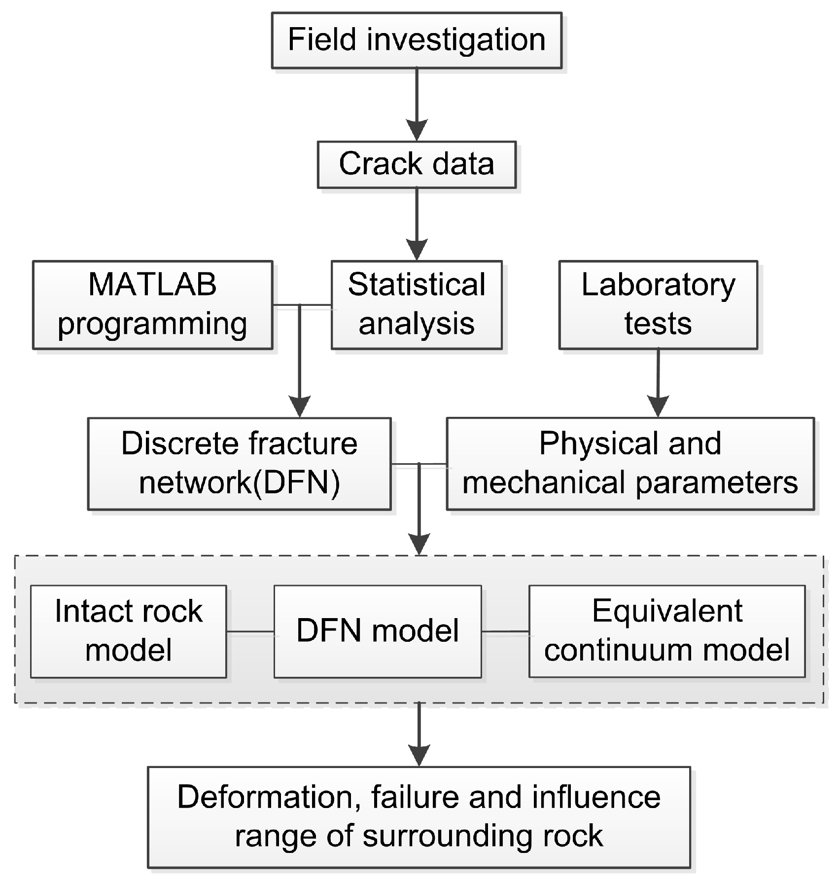
:1. Introduction
2. Crack Investigation and Distribution Law of the Mining Area
2.1. Geological Background
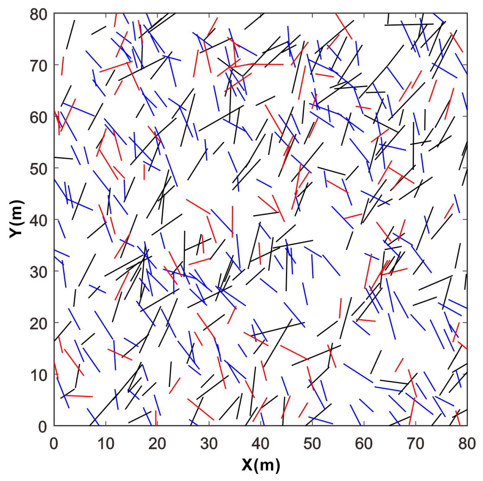
2.2. Crack Distribution
3. Physical and Mechanical Properties of the Surrounding Rocks
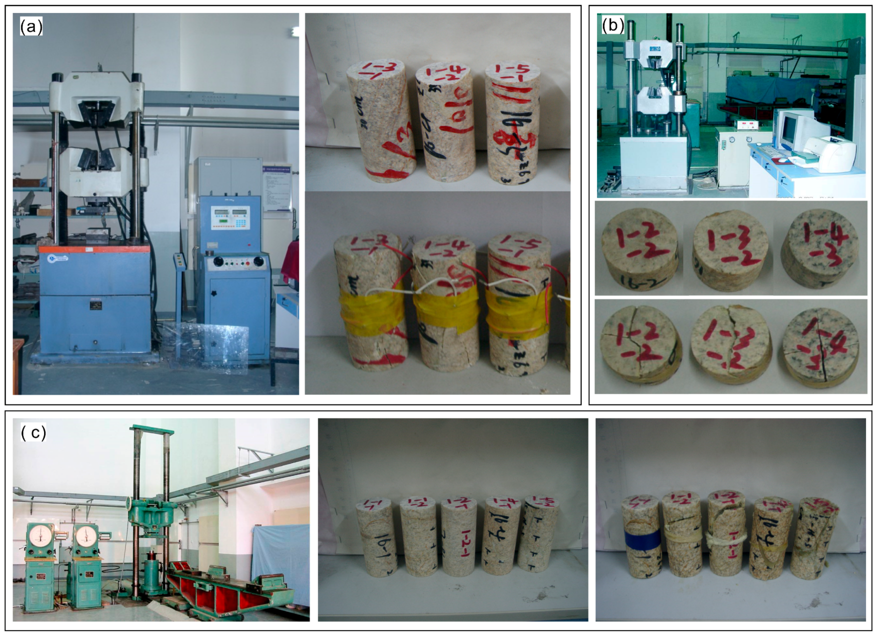
3.1. Laboratory Tests
3.2. Parameter Calibration in the Numerical Model
4. DFN Model
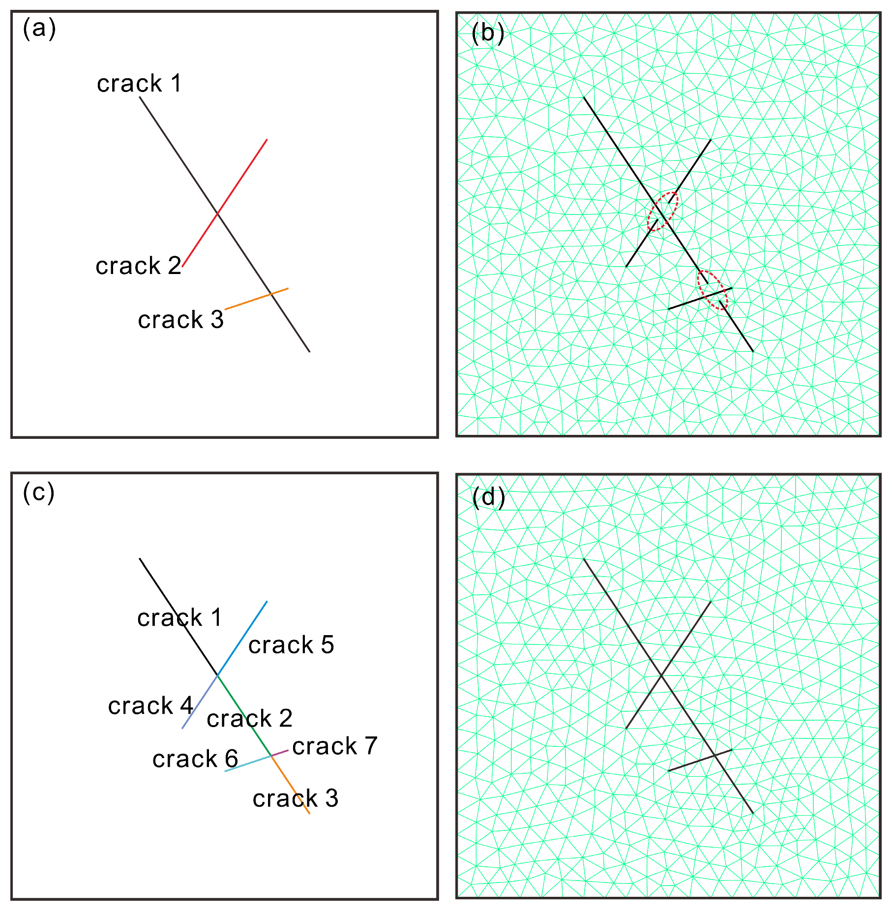
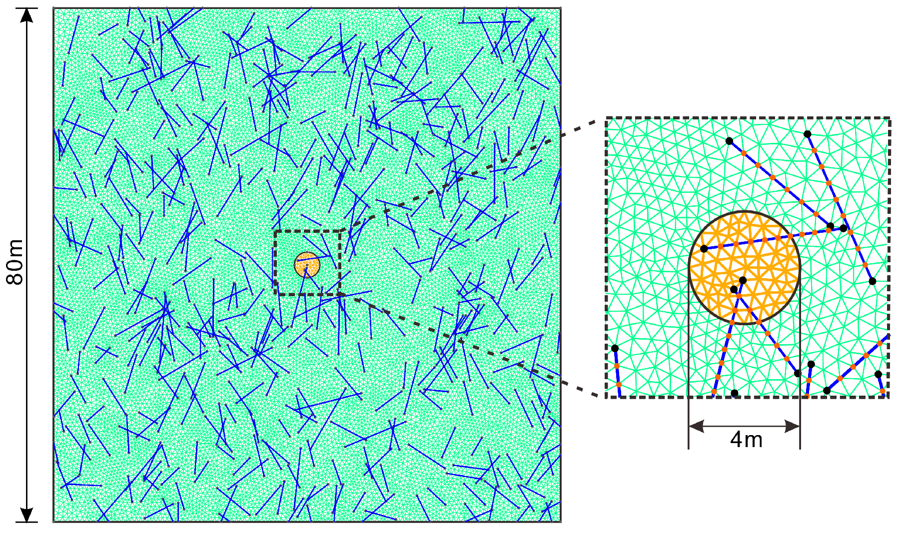
4.1. Geometry Model
4.2. Meshing of the Model
5. Influence of the DFN Model on Roadway Stability
5.1. Parameters and Scheme Designs for the Simulation
5.2. Modeling Results and Analyses
5.2.1. Deformation Features of the Roadway
5.2.2. Influence Scope of Excavation
6. Summary and Conclusions
Author Contributions
Funding
Acknowledgments
Conflicts of Interest
References
- Kamb, W.B. Ice petrofabric observations from Blue Glacier, Washington, in relation to theory and experiment. J. Geophys. Res. 1959, 64, 1891–1909. [Google Scholar] [CrossRef]
- Vollmer, F.W. C program for automatic contouring of spherical orientation data using a modified Kamb method. Comput. Geosci. 1995, 21, 31–49. [Google Scholar] [CrossRef]
- Wu, F.Q. Principles of Statistical Mechanics of Rock Masses; China University of Geosciences Press: Wuhan, China, 1993. [Google Scholar]
- Chen, J.P. 3-D network numerical modeling technique for random discontinuities of rock mass. Chin. J. Geotech. Eng. 2001, 23, 397–402. [Google Scholar]
- Li, S.; Tang, D.; Xu, H.; Yang, Z. Advanced characterization of physical properties of coals with different coal structures by nuclear magnetic resonance and X-ray computed tomography. Comput. Geosci. 2012, 48, 220–227. [Google Scholar] [CrossRef]
- Xie, J.; Gao, M.Z.; Zhang, R. Quantitative description methods and anisotropic characteristics of reconstructed DFN model. Chin. J. Geotech. Eng. 2016, 38, 98–103. [Google Scholar]
- Kulatilake, P.; Wu, T.H. Estimation of mean trace length of discontinuities. Rock Mech. Rock Eng. 1984, 17, 215–232. [Google Scholar] [CrossRef]
- Priest, S.D.; Hudson, J.A. Discontinuity spacings in rock. Int. J. Rock Mech. Min. Sci. Geomech. Abstr. 1976, 13, 135–148. [Google Scholar] [CrossRef]
- Dverstorp, B.; Andersson, J. Application of the discrete fracture network concept with field data: Possibilities of model calibration and validation. Water Resour. Res. 1989, 25, 540–550. [Google Scholar] [CrossRef]
- Baghbanan, A.; Jing, L. Stress effects on permeability in a fractured rock mass with correlated fracture length and aperture. Int. J. Rock Mech. Min. Sci. 2008, 45, 1320–1334. [Google Scholar] [CrossRef]
- Liu, R.C.; Jiang, Y.J.; Li, B. Numerical calculation of directivity of equivalent permeability of fractured rock masses network. Rock Soil Mech. 2014, 35, 2394–2400. [Google Scholar]
- Yao, C.; Zhao, M.; Yang, J.H. A coupled RBSM-DFN model for simulating hydraulic fracturing. Chin. J. Rock Mech. Eng. 2018, 37, 1438–1445. [Google Scholar]
- Song, X.M.; Gu, T.F.; Liu, C.W. Experimental study on roadway stability in rock mass with connected fissures. Chin. J. Rock Mech. Eng. 2002, 21, 1781–1785. [Google Scholar]
- Elmo, D.; Stead, D. An integrated numerical modelling–discrete fracture network approach applied to the characterisation of rock mass strength of naturally fractured pillars. Rock Mech. Rock Eng. 2010, 43, 3–19. [Google Scholar] [CrossRef]
- Huang, D.; Li, X.Q. Research on representative elementary volume based on discrete fracture network. Eng. J. Wuhan Univ. 2016, 750–755. [Google Scholar]
- Liu, X.L.; Lin, P.; Han, G.F. Hydro-mechanical coupling process on rock slope stability based on discontinuous deformation analysis and discrete fracture network models. Chin. J. Rock Mech. Eng. 2013, 32, 1248–1256. [Google Scholar]
- Guo, J.; Ma, F.S.; Zhao, H.J. Preferred seepage channels and source of water inrush in seabed gold mine at Sanshandao. J. Eng. Geol. 2015, 23, 784–789. [Google Scholar]
- Li, S.H.; Wang, J.G.; Liu, B.S. Analysis of critical excavation depth for a jointed rock slope using a face-to-face discrete element method. Rock Mech. Rock Eng. 2007, 40, 331–348. [Google Scholar] [CrossRef]
- Feng, C.; Li, S.; Wang, J. Stability analysis method for bedding rock slopes under seismic load. Chin. J. Geotech. Eng. 2012, 22, 717–724. [Google Scholar]
- Hudson, J.A.; Crouch, S.L.; Fairhurst, C. Soft, stiff and servo-controlled testing machines: A review with reference to rock failure. Eng. Geol. 1972, 6, 155–189. [Google Scholar] [CrossRef]
- Carpinteri, A. Fractal nature of material microstructure and size effects on apparent mechanical properties. Mech. Mater. 1994, 18, 89–101. [Google Scholar] [CrossRef]
- Guo, Z. The mechanical characteristics of mine-controlled fault F1 on Sanshandao gold mine and reinforcement measures. J. Eng. Geol. 1994, 2, 23–30. [Google Scholar]
- Miao, S.J.; Wan, L.H.; Lai, X.P. Relation analysis between in situ stress field and geological tectonism in Sanshandao Gold Mine. Chin. J. Rock Mech. Eng. 2004, 23, 3996–3999. [Google Scholar]


| Set of Cracks | Set 1 | Set 2 | Set 3 | |
|---|---|---|---|---|
| Number of Cracks | 451 | 453 | 216 | |
| Inclination | Distribution law | Gaussian normal | Gaussian normal | Uniform |
| Range (°) | (30, 200) | (0, 30), (200, 360) | (−10, 70), (170, 250) | |
| Expectation (°) | 123 | 297 | - | |
| Standard deviation (°) | 28.7 | 38.2 | - | |
| Dip | Distribution law | Gaussian normal | Gaussian normal | Uniform |
| Range (°) | (0, 90) | (0, 90) | (70, 90) | |
| Expectation (°) | 68 | 62 | - | |
| Standard deviation (°) | 25.2 | 18.6 | - | |
| Lithology | Density (g·cm–3) | Brazilian Split Test | Uniaxial Compression Test | Triaxial Compression Test | |||
|---|---|---|---|---|---|---|---|
| Tensile Strength (MPa) | Uniaxial Compression Strength (MPa) | Young’s Modulus (GPa) | Poisson’s Ratio | Cohesion (MPa) | Friction Angle (°) | ||
| Sericite-Quartz Granitic Cataclastic Rock | 2.627 | 3.43 | 27.73 | 7.13 | 0.120 | 10.98 | 46.25 |
| 2.620 | 5.69 | 41.97 | 23.38 | 0.197 | |||
| - | 6.62 | 63.24 | 22.08 | 0.348 | |||
| Mean Value of Properties | 2.624 | 5.25 | 44.31 | 17.53 | 0.222 | - | - |
| Parameter | Normal Stiffness (Pa/m) | Shear Stiffness (Pa/m) | Friction Angle (°) | Cohesion (MPa) | Tensile Strength (MPa) | Tensile Fracture Energy (Pa·m) | Shear Fracture Energy (Pa·m) |
|---|---|---|---|---|---|---|---|
| Value | 2 × 10¹³ | 2 × 10¹³ | 40 | 9.8 | 4.8 | 20 | 140 |
| Parameters for Scheme 1 and 2 | Parameters for Scheme 3 | Parameters of DFN for Scheme 2 | |||
|---|---|---|---|---|---|
| Set 1 and 2 | Set 3 | ||||
| Block Elements | Young’s modulus (GPa) | 1.75 | 0.88 | - | - |
| Poisson’s ratio (-) | 0.20 | 0.20 | - | - | |
| Density (g·cm−3) | 2.60 | 2.60 | - | - | |
| Cohesion (MPa) | 1.01 | 1.00 | - | - | |
| Friction angle (°) | 35 | 25 | - | - | |
| Tensile strength (MPa) | 0.52 | 0.50 | - | - | |
| Springs | Cohesion (MPa) | 1.10 | 1.00 | 1.40 × 10⁻² | 7.00 × 10⁻³ |
| Friction angle (°) | 30 | 22 | 10 | 10 | |
| Tensile strength (MPa) | 0.52 | 0.50 | 7.00 × 10⁻³ | 3.50 × 10⁻³ | |
| Normal stiffness (Pa/m) | 2 × 10¹² | 1 × 10¹² | 5 × 10¹⁰ | 5 × 10¹⁰ | |
| Shear stiffness (Pa/m) | 2 × 10¹² | 1 × 10¹² | 5 × 10¹⁰ | 5 × 10¹⁰ | |
| Tensile fracture energy (Pa·m) | 10.0 | 8.0 | 0.2 | 0.1 | |
| Shear fracture energy (Pa·m) | 60.0 | 48.0 | 1.2 | 0.6 | |
© 2019 by the authors. Licensee MDPI, Basel, Switzerland. This article is an open access article distributed under the terms and conditions of the Creative Commons Attribution (CC BY) license (http://creativecommons.org/licenses/by/4.0/).
Share and Cite
Liu, G.; Ma, F.; Zhao, H.; Li, G.; Cao, J.; Guo, J. Study on the Fracture Distribution Law and the Influence of Discrete Fractures on the Stability of Roadway Surrounding Rock in the Sanshandao Coastal Gold Mine, China. Sustainability 2019, 11, 2758. https://0-doi-org.brum.beds.ac.uk/10.3390/su11102758
Liu G, Ma F, Zhao H, Li G, Cao J, Guo J. Study on the Fracture Distribution Law and the Influence of Discrete Fractures on the Stability of Roadway Surrounding Rock in the Sanshandao Coastal Gold Mine, China. Sustainability. 2019; 11(10):2758. https://0-doi-org.brum.beds.ac.uk/10.3390/su11102758
Chicago/Turabian StyleLiu, Gang, Fengshan Ma, Haijun Zhao, Guang Li, Jiayuan Cao, and Jie Guo. 2019. "Study on the Fracture Distribution Law and the Influence of Discrete Fractures on the Stability of Roadway Surrounding Rock in the Sanshandao Coastal Gold Mine, China" Sustainability 11, no. 10: 2758. https://0-doi-org.brum.beds.ac.uk/10.3390/su11102758