Renewable Power Output Forecasting Using Least-Squares Support Vector Regression and Google Data


1
Department of Industrial Engineering and Management, National Chin-Yi University of Technology, Taichung 41170, Taiwan
2
Institute of Innovation and Circular Economy, Asia University, Taichung 41354, Taiwan
3
Department of Medical Research, China Medical University Hospital, China Medical University, Taichung 40402, Taiwan
4
Department of Information Management, Lunghwa University of Science and Technology, Taoyuan 33306, Taiwan
5
Department of Industrial Engineering and Enterprise Information, Tunghai University, Taichung 40704, Taiwan
*
Author to whom correspondence should be addressed.
Sustainability 2019, 11(11), 3009; https://0-doi-org.brum.beds.ac.uk/10.3390/su11113009
Submission received: 10 May 2019
/
Revised: 21 May 2019
/
Accepted: 22 May 2019
/
Published: 28 May 2019
Abstract
:Sustainable and green technologies include renewable energy sources such as solar power, wind power, and hydroelectric power. Renewable power output forecasting is an essential contributor to energy technology and strategy analysis. This study attempts to develop a novel least-squares support vector regression with a Google (LSSVR-G) model to accurately forecast power output with renewable power, thermal power, and nuclear power outputs in Taiwan. This study integrates a Google application programming interface (API), least-squares support vector regression (LSSVR), and a genetic algorithm (GA) to develop a novel LSSVR-G model for accurately forecasting power output from various power outputs in Taiwan. Material price and the search volume via Google’s search engine for keywords, which is used for various power outputs and is collected by Google APIs, are used as input data. The forecasting model uses LSSVR. Furthermore, the LSSVR employs a GA to find the optimal parameters for the LSSVR. Real-world annual power output datasets collected from Taiwan were used to demonstrate the forecasting performance of the model. The empirical results reveal that the proposed LSSVR-G model is superior to all other considered models both in terms of accuracy and stability, and, thus, can be a useful tool for renewable power forecasting. Moreover, the accuracy forecasting thermal power and nuclear power could effectively assist in understanding the future trend of renewable power output in Taiwan. The accurately forecasting result could effectively provide basic information for renewable power, thermal power, and nuclear power planning and policy making in Taiwan.
1. Introduction
Governments currently promote methods of electricity generation with high efficiency, minimal pollution, and greenhouse gas emissions in accordance with the United Nations’ Sustainable Development Goals (SDGs). Sustainable and green technologies have been widely studied, including non-dispatched renewable energy sources such as solar power and wind power. However, thermal and nuclear power outputs still contribute a higher percentage toward industry and public requirements in Taiwan. Governments need to engage in long-term planning for electricity generation. Therefore, an accurate forecasting system is needed for governments to efficiently plan the future distribution of power generation. Material price and government policy influence thermal power and nuclear power generations. Moreover, renewable power generation mainly depends on government policy and public expectations, and the trend of thermal power and nuclear power outputs would influence the renewable power generation. Therefore, this study develops a forecasting model for observing the changes in annual power output in Taiwan combining the least-squares support vector regression with google (LSSVR-G).
In recent times, many researchers have studied the power output forecasting problem. Shi et al. [1] developed a hybrid model that forecasts wind power output 15 min ahead of time and is based on grey relational analysis and wind speed distribution features. Their hybrid model combined a least-squares support vector machine (LSSVM) model and a radial basis function neural networks (RBFNN) model, which improves forecasting accuracy and reduced computational burden. Xu et al. [2] proposed a forecasting model that comprised a K-means clustering-based bad data detection module and a neural network (NN)-based forecasting module. Results indicated an accuracy improvement resulting from an adjustment in short-term wind power forecast detection. Zhang et al. [3] indicated that weather conditions cause solar power generation to be highly volatile. They developed and presented a similar day-based forecasting tool and analyzed the challenges of solar power forecasting. Yang et al. [4] developed a support vector machine (SVM)-enhanced Markov model for short-term wind power forecasts. Their model takes into account wind ramps, diurnal non-stationarity, and the seasonality of wind farm generation. Numerical examples showed that Yang et al.’s approach significantly improved accuracy. Li et al. [5] developed multivariate adaptive regression splines for the daily power output of a grid-connected photovoltaic system. A numerical example showed that the method outperformed artificial neural networks (ANNs), k-nearest neighbors (KNNs), classification and regression trees (CARTs), and support vector machines (SVMs). Hossain et al. [6] designed an extreme learning machine (ELM) approach to forecast three grid-connected photovoltaic systems. The proposed ELM model was judged as an acceptable and efficient machine learning approach and to be superior to support vector regression (SVR) and ANNs. Yang et al. [7] proposed a day-ahead forecasting method of photovoltaic output power with similar cloud space fusion based on incomplete historical data mining. Simulation tests based on the measured data of photovoltaic systems at a photovoltaic power station in China verified the effectiveness and correctness of the proposed method. Paulescu et al. [8] developed a black-box Takagi–Sugeno fuzzy model and a semiparametric statistical model for forecasting the output power of photovoltaic plants. Output power at time horizons of 1–72 h ahead was used as an example to examine the proposed two models. Results showed that the proposed models effectively improved predictive performance. Zjavka and Mišák [9] developed a new general differential equation that used a polynomial decomposition method for wind power forecasting. The new polynomial networks were able to describe the local atmospheric dynamics and could produce fraction substitution sum terms for all nodes. Their results indicated that midterm numerical forecasts or adaptive intelligence techniques using a local time series that outperformed all other models. Seyedmahmoudian et al. [10] used differential evolution and particle swarm optimization for a forecasting model of a polynomial (six-dimensional) form on the basis of the Maclaurin series expansion. The proposed method outperformed other methods in terms of photovoltaic output power. Rosiek et al. [11] presented a hybrid system for forecasting building-integrated photovoltaics. The system combined satellite images with a neural network. This hybrid system yielded spectacular results. Dadkhah et al. [12] proposed a hybrid system, using Kohonen’s self-organizing map (SOM) as a clustering method and radial basis function (RBF) as a classification method for accurate wind power output forecasting in a power plant. A real-world case study demonstrated the effectiveness of the proposed approach. Hao and Tain [13] used a nonlinear ensemble method and a multi-objective grey wolf optimizer algorithm for wind power forecasting. The results indicated superior performance in three real-world wind power datasets. Abuella and Chowdhury [14] showed that forecast tools could be used to manage the ramp rates of wind and solar resources. They used a post-processing adjustment approach for forecasting. The method was able to improve the capability of combined hour-ahead forecasts of solar power to capture ramp events.
Over the past few decades, the studies mentioned above have led to superior forecasting of hourly/daily power output datasets for wind and solar power. However, previous literature indicates that (1) Google data has not been widely used as a data source for forecasting problems and that (2) the yearly renewable power output dataset mainly was discussed with economic optimization strategies [15,16]. The yearly power output forecasting has not been widely investigated because of higher uncertainty. Our proposal is a prediction model that adopts LSSVR coupled with the Google API for the prediction of annual power output values. In addition, our method adopts a GA to determine the optimal parameters for LSSVR-G, which enhances performance. The rest of this paper is organized as follows. Section 2 introduces the proposed method—LSSVR with Google data—which include procedures for using the Google API and LSSVR technology. Section 3 presents the experimental results of LSSVR-G in long-term power output prediction of parameters such as renewable power, thermal power, and nuclear power outputs. Conclusions are drawn and suggestions for further research are made in Section 4.
2. LSSVR with Google
The LSSVR-G prediction model adopts the Google API for collecting public information and LSSVR technology to approach annual power output datasets. The main difference between LSSVR and support vector machines is that LSSVR adopts the minimization of the sum square errors (SSEs) of the training dataset and minimizes the margin error by an objection function. Some studies have extended the LSSVR and obtained good performance, which yields, for example, intuitionistic fuzzy LSSVR [17], twin least squares support vector regression [18], robust weighted least squares support vector regression [19], evolutionary seasonal decomposition least-square support vector regression [20], robust Lp-norm least squares support vector regression [21], and bi-sparse optimization-based least squares regression [22]. Furthermore, the LSSVR-G prediction model considers the public information that may improve the degree of accuracy while the forecasting values will be affected by public information.
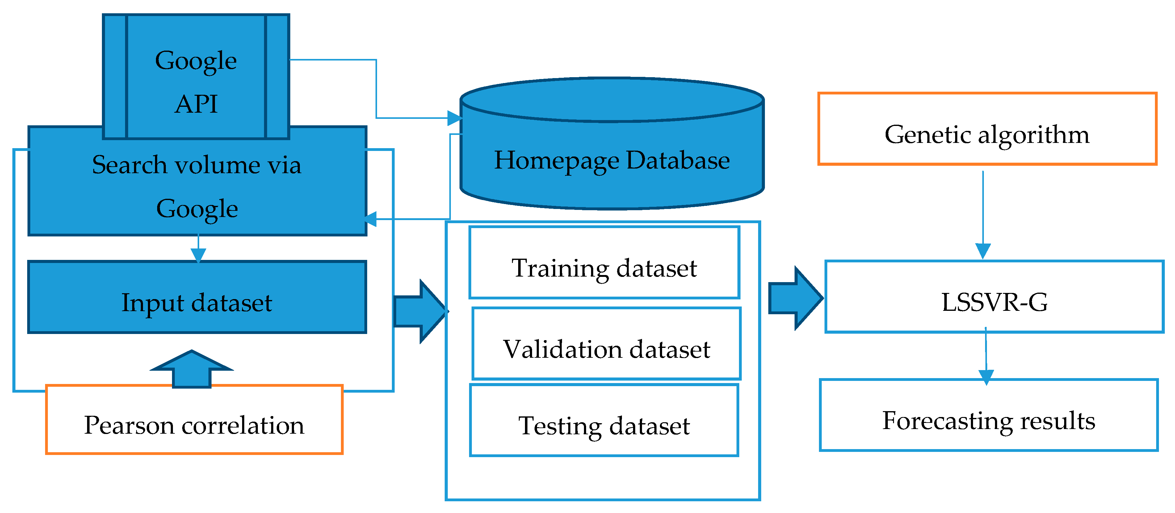
Figure 1 shows the flowchart of the proposed LSSVR-G model. The input data include yearly material prices, search volume via Google, and yearly power output are divided into three parts when using the LSSVR-G model: the training set, the validation set, and the testing set. (1) The training dataset is used to determine a proper LSSVR-G model. The input datasets were collected from the Internet, which count the number of discussion times from the Google search engine and Google plus. (2) The optimal parameter combination is determined by using the GA to train the LSSVR-G model with training data and the parameter (G) via a linear kernel function. The validation dataset is employed to search for the parameter of LSSVR-P. The negative error measure index is designed as a fitness function. (3) Based on the GA, the optimal parameters are input to examine the testing dataset and determine the predictive performance of the LSSVR-G model. The testing errors measured via root mean square error (RMSE) and mean absolute percentage error (MAPE) were calculated. The procedures of the LSSVR-P prediction model are as follows.
Step 1 (Google API): This procedure uses crawlers. (1) The Google API is employed in the LSSVR-G, which (2) extracts and places downloaded pages that generate a queue set based on input key terms. (3) Downloaded information is analyzed and compressed into a storage database via Python. (4) The process is repeated for each of the desired periods. In this study, the condition period is one year.
Step 2 (LSSVR with Google data): LSSVR is applied to the regression problem. The LSSVR-G approach is to approximate an unknown function using a training dataset {(XGi, yi), i = 1, …, N, } and following notations are adopted.
| The regression function. | |
| The feature of the inputs. | |
| ω | Coefficients of LSSVR-G. |
| β | Coefficients of LSSVR-G. |
| αi | Lagrangian multiplier vector due to the i input pattern. |
| εi | Error due to the i input pattern. |
| k(·) | The kernel function. |
The regression function can be formulated as follows.
where denotes the feature of the inputs, and ω and β indicate coefficients. Formulating the regression problem by LSSVR-G, we have the following equation.
This study adopts the Lagrangian to solve the constrained minimization problems as seen in the formula below.
where αi is the Lagrangian multiplier vector. We apply the Karush–Kuhn–Tucker conditions to provide the necessary conditions for identifying local optima of non-linear programming problems. The conditions for optimality are shown below.
In this scenario, k(XGi, XGj) denotes a kernel function whose value is equal to the inner product of two vectors, XGi and XGj, in the feature space ϕ(XGi) and ϕ(XGj), which means that k(XGi, XGj) = ϕT(XGi) ϕ(XGj). This work examines linear kernel functions in a numerical example: . We denote K = (kij)N×N, kij = k(XGi, XGj), and V = diag{1/G,1/G,…, 1/G}, so LSSVR-G can be described by the equation below.
where β = K + V. Hence, the regression model is formulated from Equation (3). The resulting LSSVR-G then becomes the equation below.
Note that, in the case of linear kernels, only one tuning parameter (G) is tested in the GA.
Step 3 (Genetic algorithm): In this study, LSSVR-G employs a GA to search for the optimal model parameters. The parameter selection is crucial for the success of the LSSVR-G model and well-chosen parameters improve LSSVR-G performance. Therefore, a GA [23,24] is used to select constant parameters (G) for the LSSVR-G.
Step 4 (Measure indexes): The root mean square error (RMSE) and MAPE were used to measure the forecasting accuracy of the model. The estimated values approached the actual values more closely than those of the RMSE or the MAPE (in percentage terms). Equations (7) and (8) illustrate the expression of the RMSE and MAPE (as a percent), respectively.
3. Numerical Examples, Experimental Results, and Discussion
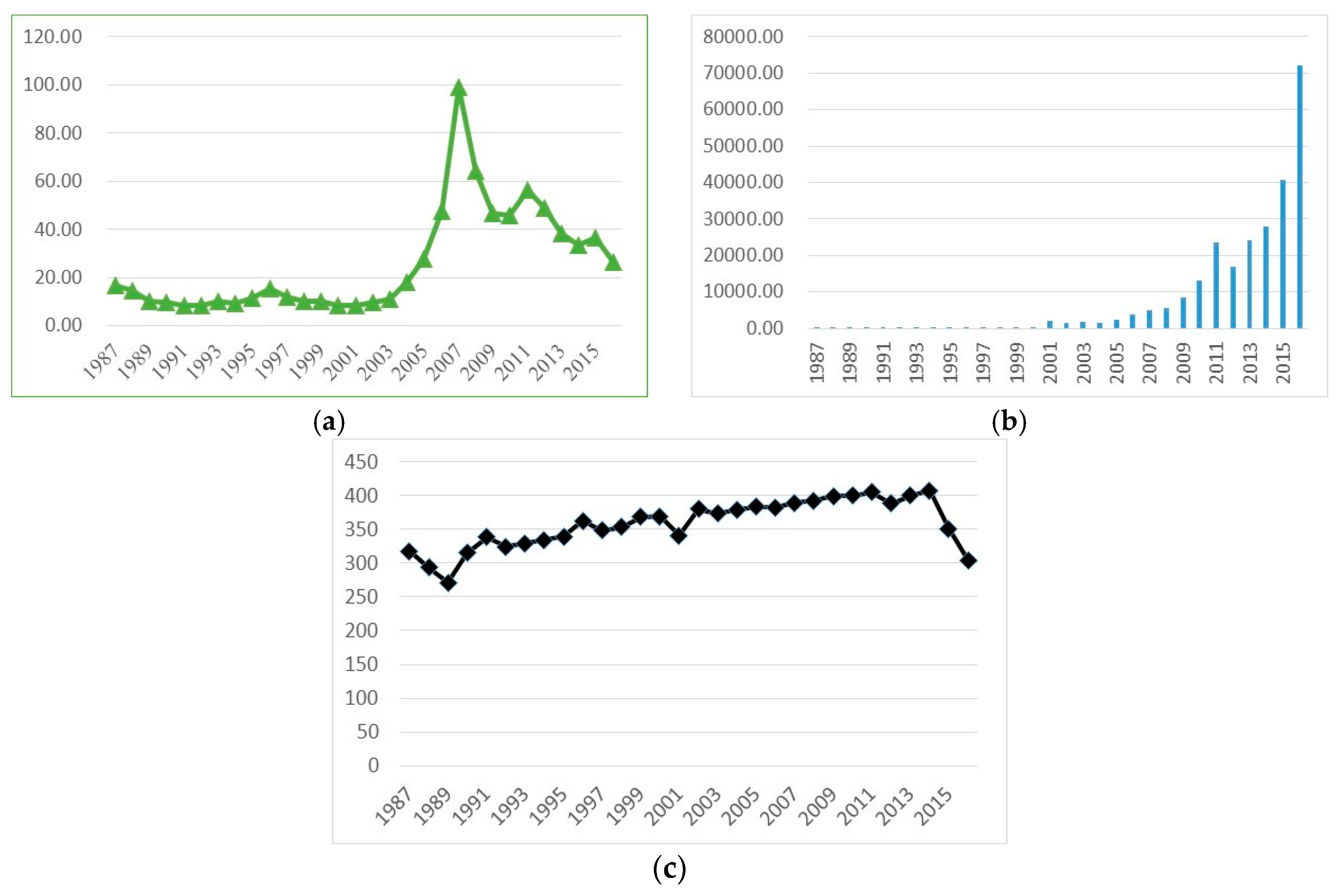
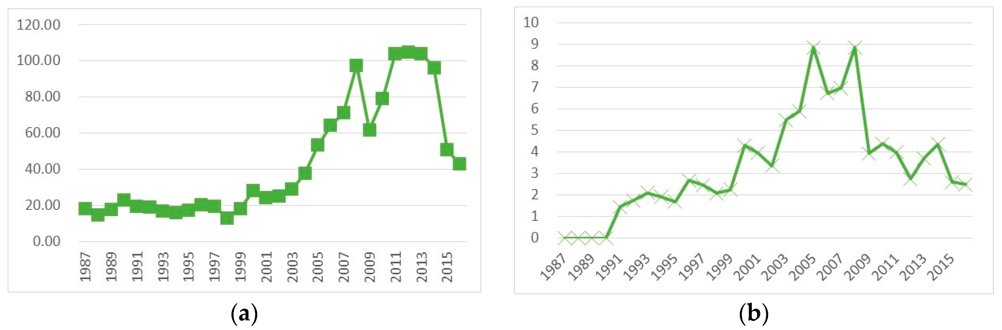
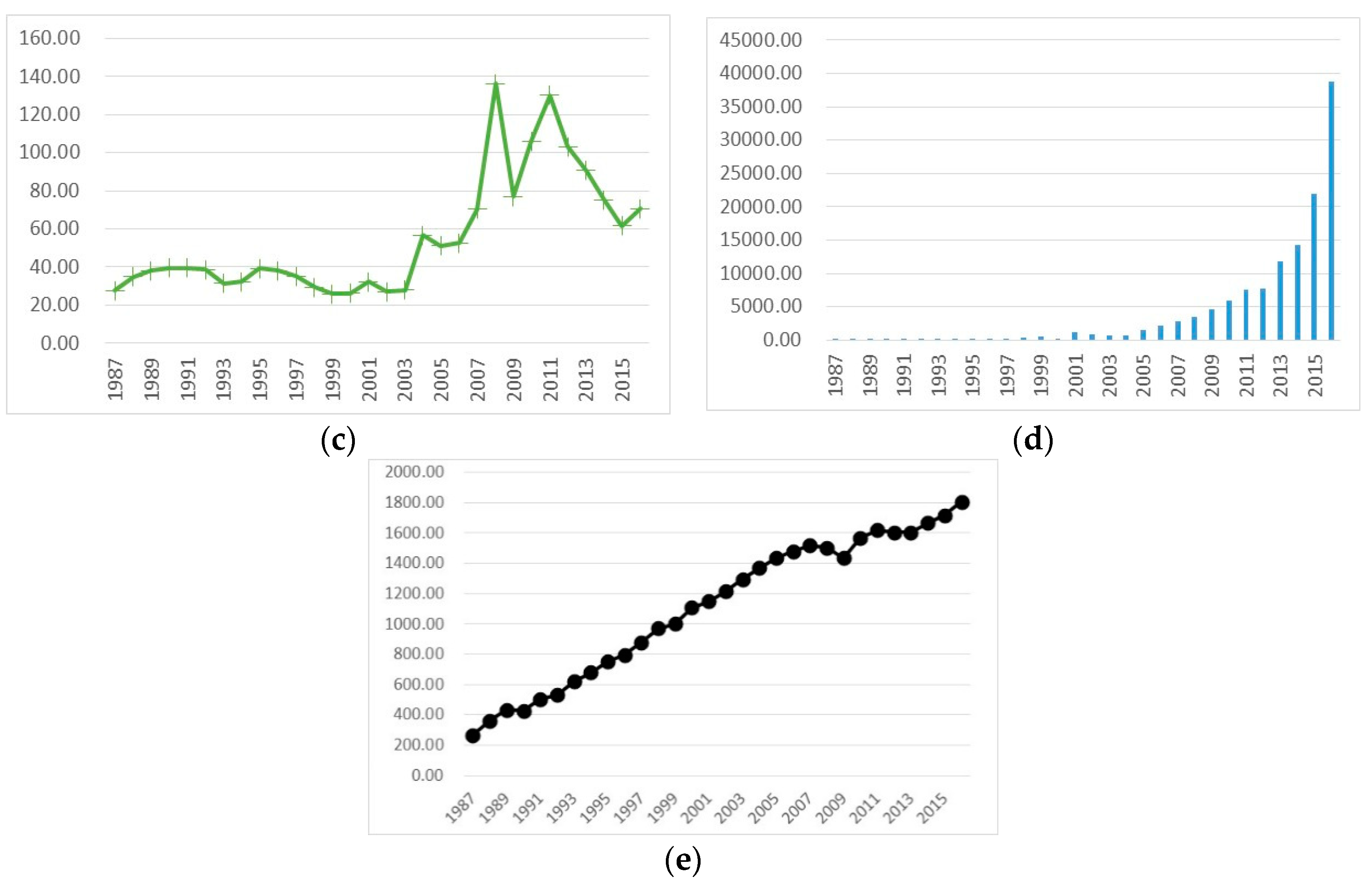
This research investigated the LSSVR-G model and its usefulness as a yearly forecast-generating mechanism with renewable power, thermal power, and nuclear power outputs from Taiwan. All yearly various power output datasets could be collected from a Taiwan power company. Figure 2, Figure 3 and Figure 4 show material prices, the search volumes via Google, and actual power output during the period from 1987 to 2016. Figure 2a–c show that the trend of uranium price decreased in the past 10 years. The trend of the search volume via Google increased and the trend of nuclear power output decreased in the past two years because of government policy. The people of Taiwan requested that a new nuclear power plant not be built during the period of 2014 to 2016. Hence, the trend of nuclear power output decreased, as shown in Figure 2c, and the search volume via Google data was larger in the past two years, as shown in Figure 2b. Figure 3a–c shows that the trend of crude oil, natural gas, and coal prices increased in the past several years. The trend of the search volume via Google for thermal power generation has also increased, as shown in Figure 3d, and the trend of thermal power output increased in the past several years, as shown in Figure 3e. This is because a nuclear power output reduction strategy was implemented in Taiwan. Figure 4a,b show that the search volume via Google increased, and the trend of renewable power increased in the past 10 years. The yearly renewable power output is the amount of the wind, solar, and hydroelectric power outputs in Taiwan.
As shown in Figure 2, Figure 3 and Figure 4, the training set covers 1987–1996, the validation set covers 1997–2006, and the testing set covers 2007–2016. Table 1 displays Pearson’s correlation coefficients between the input datasets and actual power output datasets. The search volume via Google for renewable power generation has a higher positive correlation (0.805) and is statistically significant, and total input datasets are statistically significant, except for the search volume via Google data for nuclear power generation. The reason for this phenomenon is that nuclear power generation reduces power output.
To demonstrate the superiority of the proposed LSSVR-G model, three other forecasting models—the back propagation neural network (BPNN) [25], the general regression neural network (GRNN) [26], and the autoregressive integrated moving average (ARIMA) [27]—were used for comparison. Furthermore, the LSSVR-G model in this study was also extended to LSSVR with material prices and LSSVR with both Google data and material prices, which are referred to as LSSVR-P and LSSVR-GP, respectively.
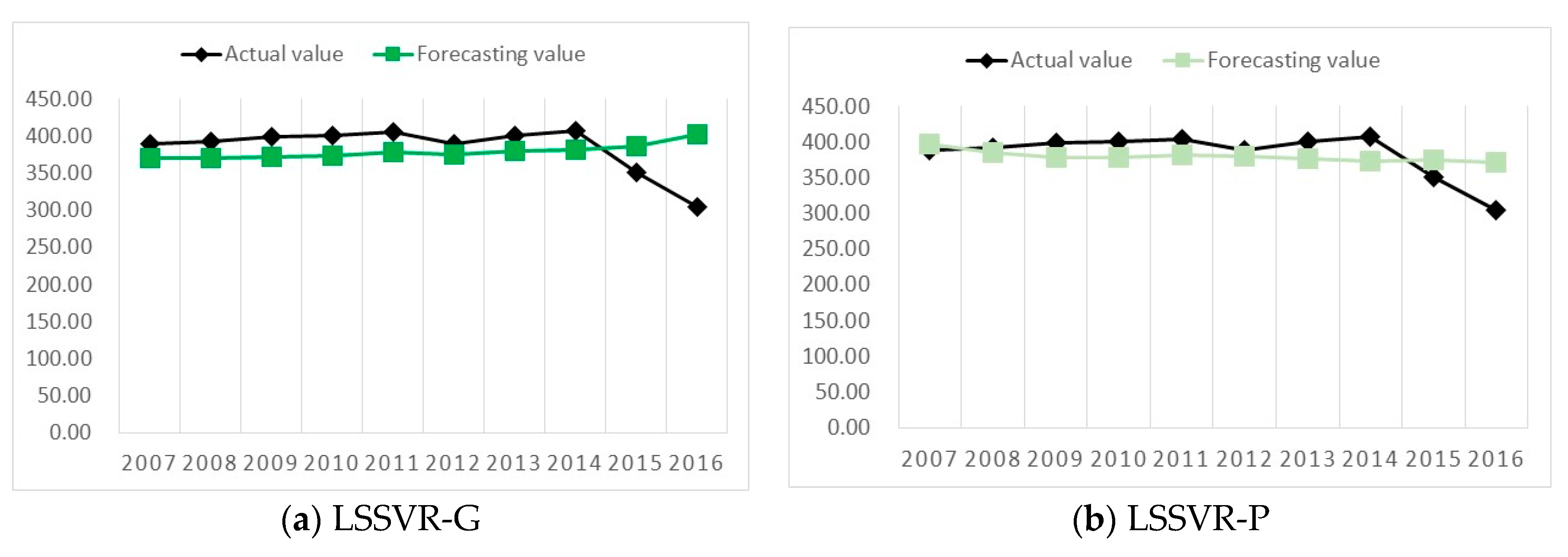
Table 2 shows the actual nuclear power output forecasting results from 2007 and 2016. It indicates that the LSSVR-P model performed better (MAPE and MSE were 6.57 and 844.03, respectively) than the compared methods. Figure 5a–f show the point-to-point comparisons of actual values and predicted values of the nuclear power output data. Based on Table 2 and Figure 5, the following were observed. First, the proposed LSSVR-G, LSSVR-P, and LSSVR-GP models outperformed the other models in terms of forecasting accuracy. MAPE was smaller than 10%. Second, LSSVR-P based on MSE obtained a superior performance to the traditional approaches (BPNN, GRNN, and ARIMA (1,1,0)) because the mechanism was extended with higher relational multi-variables. In the nuclear power output example, the uranium price had a higher relation with nuclear power output. Moreover, the GA improved the testing performance based on the optimal parameters of LSSVR-G, LSSVR-P, and LSSVR-GP. This verifies that our proposed forecasting models can assist traditional prediction models to obtain optimal performances.
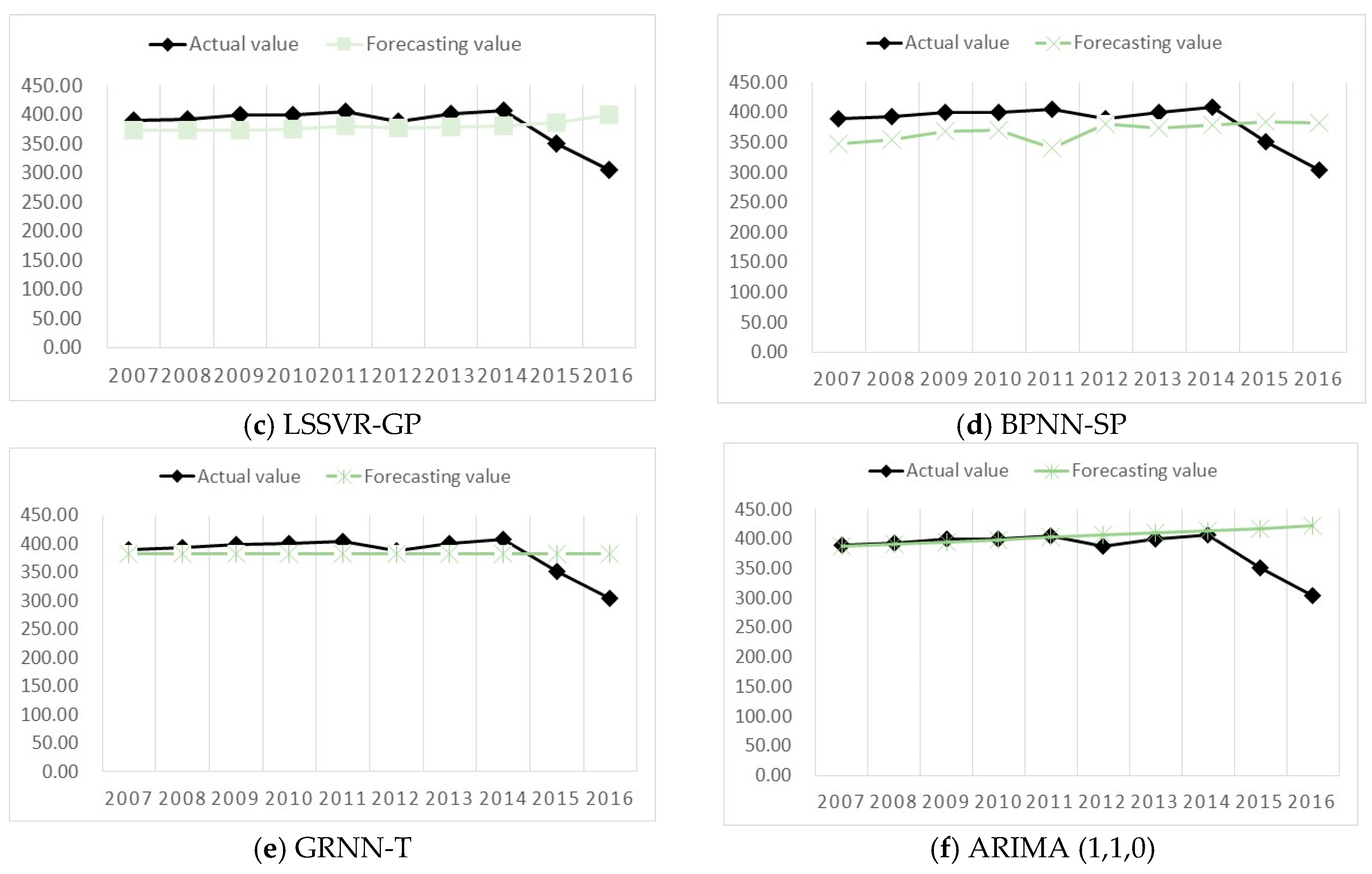
Table 3 shows the actual thermal power output forecasting results from 2007 and 2016. Table 3 indicates that the LSSVR-GP model can perform better than the compared methods (MAPE and MSE were 12.51 and 43,284.69, respectively). Figure 6a–f show the point-to-point comparisons of actual values and predicted values of the thermal power output data. Based on Table 3 and Figure 6, the following was observed. The proposed LSSVR-GP model outperformed the other models in terms of forecasting accuracy because the search volume via Google obtain high correlation for thermal power output. The material prices of thermal power generation have decreased in the last 10 years. The LSSVR-GP simultaneously considered the search volume via Google and material prices for thermal power generation. Therefore, the proposed forecasting models could more robustly predict thermal power output.
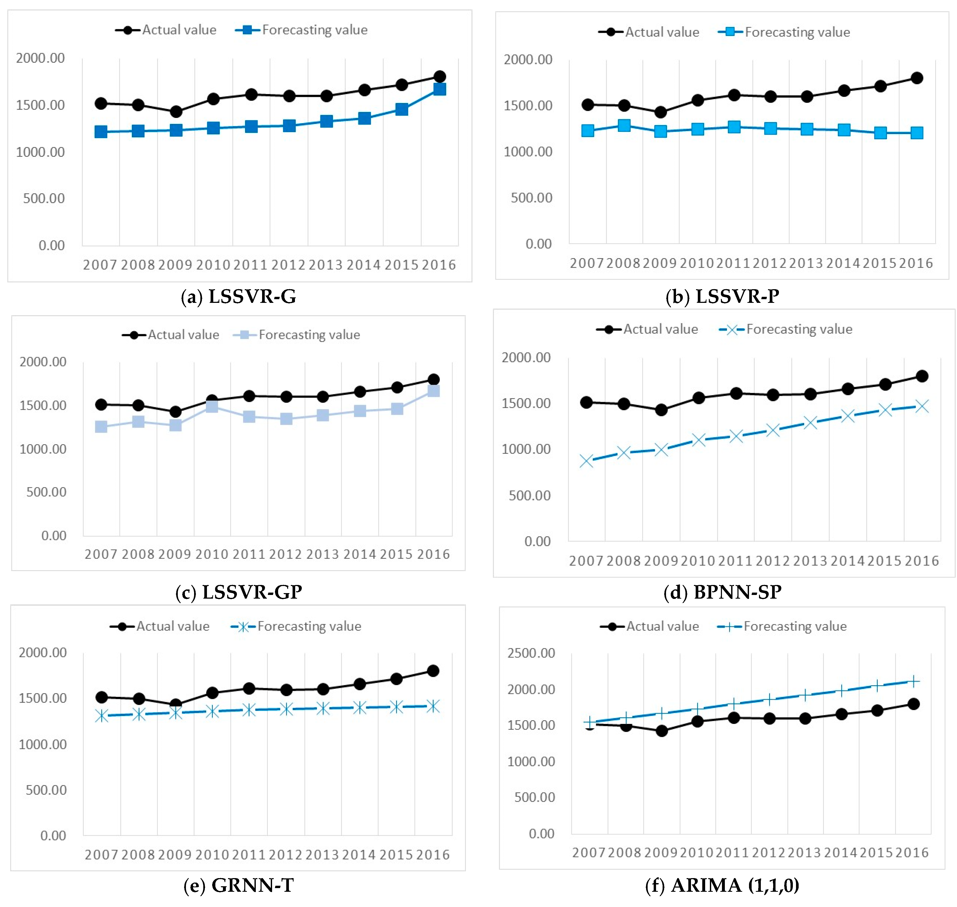
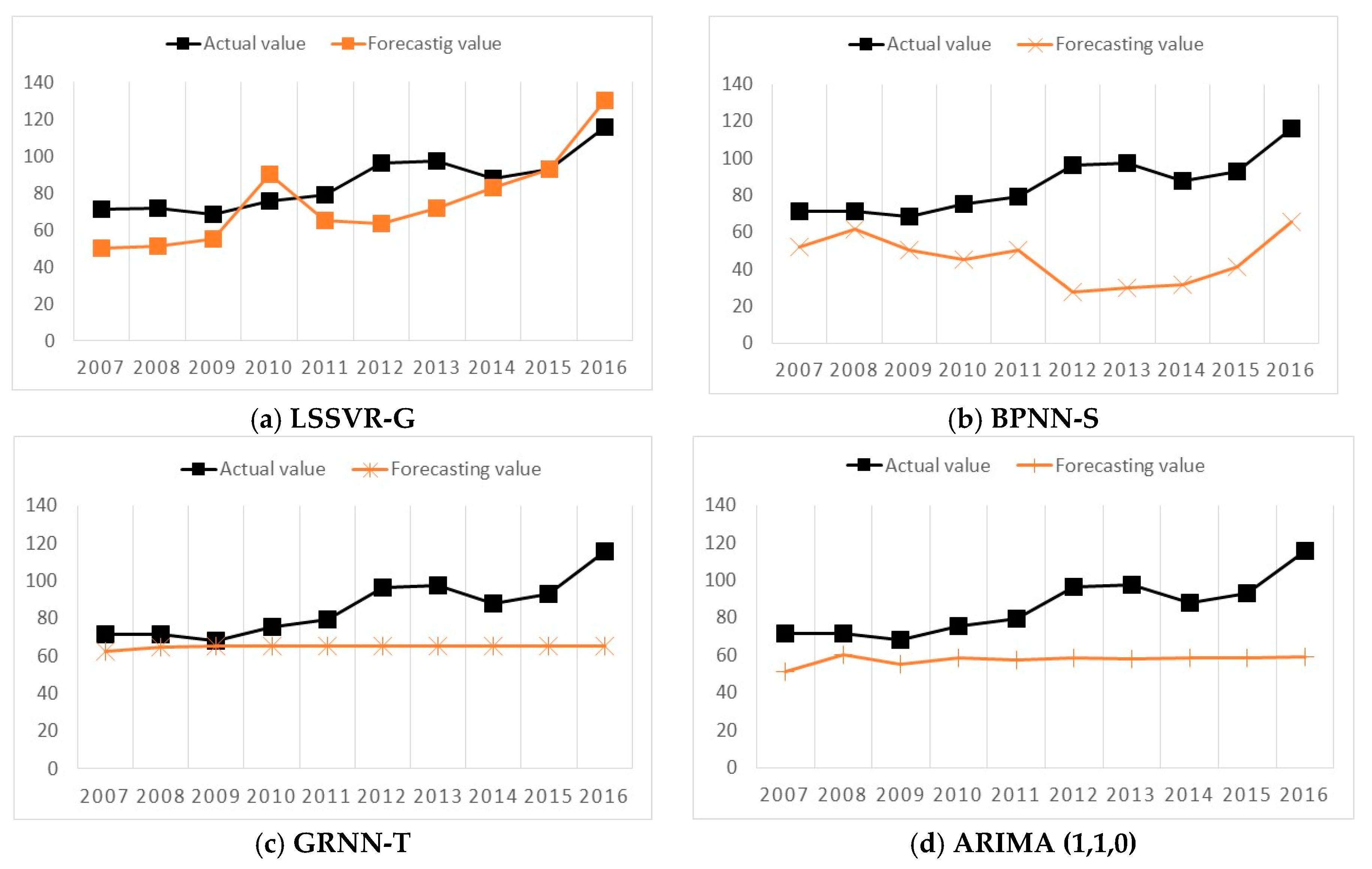
Table 4 shows the actual renewable power output forecasting results from 2007 to 2016. It indicates that the LSSVR-G model performs better than the other methods (MAPE and MSE were 19.25 and 340.46, respectively). Figure 7a–d shows the point-to-point comparisons of actual and predicted values of the renewable power output data. Based on Table 4 and Figure 7, the following was observed. For renewable power output, only the search volume via Google was considered as an input dataset, since renewable power does not require any material and utilizes only the natural environment. However, the natural environment cannot be easily controlled. The Google data mainly focused on promoting renewable power output in Taiwan. Therefore, the proposed LSSVR-G models outperformed the other models in terms of forecasting accuracy because the search volume via Google had a higher correlation with renewable power output than thermal and nuclear power output.
For assessment of power output in Taiwan, government policy, costs, and social perception should be considered. Choosing the right forecasting tool is an important factor for government and decision-makers. The LSSVR-G, LSSVR-P, and LSSVR-GP models proposed in this study provide accurate forecasts for power output generation. Our study suggests that the LSSVR-G model can be implemented to enhance renewable power output forecasting for government/decision-makers. Due to the trend of thermal power and how nuclear power outputs would influence the renewable power generation, the study suggests that the LSSVR-GP can be implemented for thermal power output, and LSSVR-P can be implemented for nuclear power output. The proposed methods can be used as an alternative forecasting tool for government and decision-makers in Taiwan. Furthermore, the forecasting results show that the renewable power output grow gradually in 2012 to 2016. The engine police promote the renewable power output that actually reflects the yearly renewable power output in Taiwan. The government will implement large investment software and hardware equipment for renewable energy based on the forecasting results.
4. Conclusions
Power output prediction is a crucial issue in many countries, and power output forecasting is an essential contributor to energy technology and strategy analysis. This study investigates the LSSVR-G, LSSVR-P, and LSSVR-GP models and their usefulness as a forecasting mechanism for power output generation. The results indicate that the LSSVR-G model is a promising alternative for forecasting power output, especially renewable power output. In addition, the LSSVR-GP model offers a promising alternative for thermal power output forecasting, and LSSVR-P offers a promising alternative model for nuclear power output. The superior performance of the LSSVR-G, LSSVR-GP, and LSSVR-GP models for renewable thermal and nuclear power output, respectively, can be attributed to two causes. First, the proposed method can efficiently capture trends in Google data via the Google API. Second, GA mechanisms can effectively improve the performance of predictions for power output forecasting. Future studies may consider using social media data to incorporate other forecasting models, such as deep learning networks.
Author Contributions
Conceptualization and methodology: K.-S.C. Methodology and writing—original draft preparation: K.-P.L. Data curation: J.-X.Y. Writing—review and editing: W.-L.H.
Funding
The Ministry of Science and Technology of the Republic of China, Taiwan, grant number MOST 107-2622-E-468-005-CC3, funded this research.
Acknowledgments
The authors would like to express appreciation to the Ministry of Science and Technology of the Republic of China, Taiwan, for financially supporting this research under Contract Numbers MOST 107-2622-E-468-005-CC3.
Conflicts of Interest
The authors declare no conflict of interest.
References
- Shi, J.; Ding, Z.; Lee, W.-J.; Yang, Y.; Liu, Y.; Zhang, M. Hybrid forecasting model for very-short term wind power forecasting based on grey relational analysis and wind speed distribution features. IEEE Trans. Smart Grid 2014, 5, 521–526. [Google Scholar] [CrossRef]
- Xu, Q.; He, D.; Zhang, N.; Kang, C.; Xia, Q.; Bai, J.; Huang, J. A Short-Term Wind Power Forecasting Approach With Adjustment of Numerical Weather Prediction Input by Data Mining. IEEE Trans. Sustain. Energy 2015, 6, 1283–1291. [Google Scholar] [CrossRef]
- Zhang, Y.; Beaudin, M.; Taheri, R.; Zareipour, H.; Wood, D. Day-Ahead Power Output Forecasting for Small-Scale Solar Photovoltaic Electricity Generators. IEEE Trans. Smart Grid 2015, 6, 2253–2262. [Google Scholar] [CrossRef]
- Yang, L.; He, M.; Zhang, J.; Vittal, V. Support-Vector-Machine-Enhanced Markov Model for Short-Term Wind Power Forecast. IEEE Trans. Sustain. Energy 2015, 6, 791–799. [Google Scholar] [CrossRef]
- Li, Y.; He, Y.; Su, Y.; Shu, L. Forecasting the daily power output of a grid-connected photovoltaic system based on multivariate adaptive regression splines. Appl. Energy 2016, 180, 392–401. [Google Scholar] [CrossRef]
- Hossain, M.; Mekhilef, S.; Danesh, M.; Olatomiwa, L.; Shamshirband, S. Application of extreme learning machine for short term output power forecasting of three grid-connected PV systems. J. Clean. Prod. 2017, 167, 395–405. [Google Scholar] [CrossRef]
- Yang, X.; Xu, M.; Xu, S.; Han, X. Day-ahead forecasting of photovoltaic output power with similar cloud space fusion based on incomplete historical data mining. Appl. Energy 2017, 206, 683–696. [Google Scholar] [CrossRef]
- Paulescu, M.; Brabec, M.; Boata, R.; Badescu, V. Structured, physically inspired (gray box) models versus black box modeling for forecasting the output power of photovoltaic plants. Energy 2017, 121, 792–802. [Google Scholar] [CrossRef]
- Zjavka, L.; Mišák, S. Direct Wind Power Forecasting Using a Polynomial Decomposition of the General Differential Equation. IEEE Trans. Sustain. Energy 2018, 9, 1529–1539. [Google Scholar] [CrossRef]
- Seyedmahmoudian, M.; Jamei, E.; Thirunavukkarasu, G.S.; Soon, T.K.; Mortimer, M.; Horan, B.; Stojcevski, A.; Mekhilef, S. Short-Term Forecasting of the Output Power of a Building-Integrated Photovoltaic System Using a Metaheuristic Approach. Energies 2018, 11, 1260. [Google Scholar] [CrossRef]
- Rosiek, S.; Alonso-Montesinos, J.; Batlles, F.J. Online 3-h forecasting of the power output from a BIPV system using satellite observations and ANN. Electr. Power Energy Syst. 2018, 99, 261–272. [Google Scholar] [CrossRef]
- Dadkhah, M.; Rezaee, M.J.; Chavoshi, A.Z. Short-term power output forecasting of hourly operation in power plant based on climate factors and effects of wind direction and wind speed. Energy 2018, 148, 775–788. [Google Scholar] [CrossRef]
- Hao, Y.; Tian, C. A novel two-stage forecasting model based on error factor and ensemble method for multi-step wind power forecasting. Appl. Energy 2019, 238, 368–383. [Google Scholar] [CrossRef]
- Abuella, M.; Chowdhury, B. Forecasting of solar power ramp events: A post-processing approach. Renew. Energy 2019, 133, 1380–1392. [Google Scholar] [CrossRef]
- Kasperowicz, R.; Pinczyński, M.; Khabdullin, A. Modeling the power of renewable energy sources in the context of classical electricity system transformation. J. Int. Stud. 2017, 10, 264–272. [Google Scholar] [CrossRef]
- Shayesteh, E.; Yu, J.; Hilber, P. Maintenance optimization of power systems with renewable energy sources integrated. Energy 2018, 149, 577–586. [Google Scholar] [CrossRef]
- Hung, K.-C.; Lin, K.-P. Long-term business cycle forecasting through a potential intuitionistic fuzzy least-squares support vector regression approach. Inf. Sci. 2013, 224, 37–48. [Google Scholar] [CrossRef]
- Zhao, Y.-P.; Zhao, J.; Zhao, M. Twin least squares support vector regression. Neurocomputing 2013, 118, 225–236. [Google Scholar] [CrossRef]
- Chen, C.; Yan, C.; Li, Y. A robust weighted least squares support vector regression based on least trimmed squares. Neurocomputing 2015, 168, 941–946. [Google Scholar] [CrossRef]
- Lin, K.-P.; Pai, P.-F. Solar power output forecasting using evolutionary seasonal decomposition least-square support vector regression. J. Clean. Prod. 2016, 134, 456–462. [Google Scholar] [CrossRef]
- Ye, Y.-F.; Shao, Y.-H.; Deng, N.-Y.; Li, C.-N.; Hua, X.-Y. Robust Lp-norm least squares support vector regression with feature selection. Appl. Math. Comput. 2017, 305, 32–52. [Google Scholar] [CrossRef]
- Zhang, Z.; He, J.; Gao, G.; Tian, Y. Bi-sparse optimization-based least squares regression. Appl. Soft Comput. J. 2019, 77, 300–315. [Google Scholar] [CrossRef]
- Holland, H. Adaptation in Natural and Artificial System; University of Michigan Press: Ann Arbor, MI, USA, 1975. [Google Scholar]
- Lin, K.-P.; Pai, P.-F.; Yang, S.-L. Forecasting concentrations of air pollutants by support vector regression models with data preprocessing procedures and immune algorithms. Appl. Math. Comput. 2011, 217, 5318–5327. [Google Scholar]
- Rumelhart, D.E.; Hinton, G.E.; Williams, R.J. Learning representations by back-propagating errors. Nature 1986, 323, 533–536. [Google Scholar] [CrossRef]
- Specht, D.F. A general regression neural network. IEEE Trans. Neural Netw. 1991, 2, 568–576. [Google Scholar] [CrossRef] [PubMed]
- Box, G.; Jenkins, G. Time Series Analysis: Forecasting and Control; Holden-Day: San Francisco, CA, USA, 1976. [Google Scholar]
Figure 1.
A flowchart of the LSSVR-G prediction model.

Figure 2.
Illustration of actual values from 1987 to 2016 for nuclear power output. (a) Uranium price (US$/pound). (b) Search volume via Google related to nuclear power generation. (c) Actual nuclear power output (Giga watts, GW).
Figure 2.
Illustration of actual values from 1987 to 2016 for nuclear power output. (a) Uranium price (US$/pound). (b) Search volume via Google related to nuclear power generation. (c) Actual nuclear power output (Giga watts, GW).

Figure 3.
Illustration of actual values from 1987 to 2016 for thermal power output. (a) Crude oil price (US$/barrel). (b) Natural gas price (US$/million British thermal units). (c) Coal price (US$/Metric tons). (d) Search volume via Google for thermal power generation. (e) Actual thermal power output (GW).


Figure 4.
Illustration of actual values from 1987 to 2016 for renewable power output. (a) Search volume via Google for renewable power generation. (b) Actual renewable power output (GW).
Figure 4.
Illustration of actual values from 1987 to 2016 for renewable power output. (a) Search volume via Google for renewable power generation. (b) Actual renewable power output (GW).

Figure 5.
Illustration of actual values and forecasting values (GW/Year) of various models for nuclear power output.
Figure 5.
Illustration of actual values and forecasting values (GW/Year) of various models for nuclear power output.


Figure 6.
Illustration of actual values and forecasting values (GW/Year) of various models for thermal power output.
Figure 6.
Illustration of actual values and forecasting values (GW/Year) of various models for thermal power output.

Figure 7.
Illustration of actual values and forecasting values (GW/Year) of various models for renewable power output.
Figure 7.
Illustration of actual values and forecasting values (GW/Year) of various models for renewable power output.


Table 1.
Pearson’s correlation coefficients between input datasets and actual power output datasets.
Table 1.
Pearson’s correlation coefficients between input datasets and actual power output datasets.
| Search Volume via Google | Crude Oil Price | Natural Gas Price | Coal Price | Uranium Price | |||
|---|---|---|---|---|---|---|---|
| Renewable Power Generation | Thermal Power Generation | Nuclear Power Generation | Thermal Power Generation | Nuclear Power Generation | |||
| Pearson Correlation | 0.805 | 0.612 | 0.079 | 0.780 | 0.530 | 0.665 | 0.585 |
| p-value | 0.000 * | 0.000* | 0.677 | 0.000 * | 0.005 * | 0.000 * | 0.001 * |
* p-value < 0.05.
Table 2.
Comparison of the forecasting results for nuclear power output.
| Actual Value (GW/Year) | LSSVR-G | LSSVR-P | LSSVR-GP | BPNN-SP | GRNN | ARIMA | |
|---|---|---|---|---|---|---|---|
| 2007 | 389.61 | 369.94 | 397.88 | 374.06 | 348.46 | 383.25 | 388.26 |
| 2008 | 392.60 | 370.32 | 385.35 | 372.62 | 354.08 | 383.19 | 391.71 |
| 2009 | 399.81 | 371.66 | 379.09 | 372.96 | 369.07 | 383.17 | 395.61 |
| 2010 | 400.29 | 373.96 | 378.84 | 375.04 | 369.96 | 383.17 | 399.38 |
| 2011 | 405.22 | 378.92 | 382.51 | 380.16 | 340.94 | 383.17 | 403.19 |
| 2012 | 388.87 | 375.79 | 379.89 | 376.89 | 380.09 | 383.17 | 406.99 |
| 2013 | 400.79 | 379.26 | 376.20 | 379.56 | 373.71 | 383.17 | 410.79 |
| 2014 | 408.01 | 381.04 | 374.39 | 380.95 | 379.39 | 383.17 | 414.60 |
| 2015 | 351.43 | 387.21 | 375.55 | 386.81 | 384.04 | 383.17 | 418.40 |
| 2016 | 304.61 | 402.29 | 371.82 | 400.22 | 383.17 | 383.17 | 422.20 |
| MAPE | 8.84 | 6.57 | 8.47 | 10.26 | 6.46 | 6.87 | |
| MSE | 1524.26 | 844.03 | 1434.62 | 1803.84 | 932.38 | 1881.08 | |
| Ranking | (4) | (1) | (3) | (5) | (2) | (6) |
Table 3.
Comparison of the forecasting results for thermal power output.
| Actual Value (GW/Year) | LSSVR-G | LSSVR-P | LSSVR-GP | BPNN-SP | GRNN | ARIMA | |
|---|---|---|---|---|---|---|---|
| 2007 | 1518.27 | 1213.94 | 1235.88 | 1257.94 | 878.59 | 1317.19 | 1550.41 |
| 2008 | 1503.57 | 1223.05 | 1290.14 | 1317.98 | 969.73 | 1335.09 | 1609.63 |
| 2009 | 1434.94 | 1237.58 | 1223.18 | 1275.14 | 999.37 | 1351.08 | 1675.27 |
| 2010 | 1567.55 | 1254.98 | 1248.43 | 1489.93 | 1106.72 | 1365.25 | 1737.82 |
| 2011 | 1616.92 | 1275.35 | 1271.85 | 1375.16 | 1148.22 | 1377.73 | 1801.86 |
| 2012 | 1602.47 | 1277.79 | 1253.74 | 1349.59 | 1215.26 | 1388.67 | 1865.18 |
| 2013 | 1604.27 | 1329.04 | 1250.40 | 1392.58 | 1295.66 | 1398.25 | 1928.85 |
| 2014 | 1665.27 | 1360.82 | 1240.97 | 1443.23 | 1367.70 | 1406.63 | 1992.35 |
| 2015 | 1716.49 | 1459.49 | 1204.68 | 1463.51 | 1432.95 | 1413.97 | 2055.93 |
| 2016 | 1804.51 | 1675.53 | 1204.90 | 1668.29 | 1477.86 | 1420.40 | 2119.47 |
| MAPE | 17.13 | 22.16 | 12.51 | 26.23 | 13.86 | 14.17 | |
| MSE | 78,118.00 | 143,940.71 | 43,284.6 | 183,675.83 | 56,809.92 | 62,900.79 | |
| Ranking | (4) | (5) | (1) | (6) | (2) | (3) |
Table 4.
Comparison of the forecasting results for renewable power output.
| Actual Value (GW/Year) | LSSVR-G | BPNN-S | GRNN | ARIMA | |
|---|---|---|---|---|---|
| 2007 | 71.44 | 50.04 | 52.22 | 62.81 | 51.47 |
| 2008 | 71.65 | 51.46 | 61.78 | 64.88 | 60.37 |
| 2009 | 68.4 | 55.41 | 50.26 | 65.43 | 55.45 |
| 2010 | 75.54 | 90.09 | 45.41 | 65.57 | 58.82 |
| 2011 | 79.39 | 65.10 | 50.73 | 65.61 | 57.22 |
| 2012 | 96.49 | 63.62 | 27.62 | 65.62 | 58.59 |
| 2013 | 97.49 | 72.03 | 30.22 | 65.62 | 58.19 |
| 2014 | 87.87 | 82.90 | 31.99 | 65.62 | 58.85 |
| 2015 | 92.89 | 92.953 | 41.33 | 65.62 | 58.87 |
| 2016 | 115.97 | 130.19 | 65.62 | 65.62 | 59.27 |
| MAPE | 19.25 | 44.61 | 21.92 | 31.08 | |
| MSE | 340.46 | 2010.96 | 616.11 | 966.02 | |
| Ranking | (1) | (4) | (2) | (3) |
© 2019 by the authors. Licensee MDPI, Basel, Switzerland. This article is an open access article distributed under the terms and conditions of the Creative Commons Attribution (CC BY) license (http://creativecommons.org/licenses/by/4.0/).
Share and Cite
MDPI and ACS Style
Chen, K.-S.; Lin, K.-P.; Yan, J.-X.; Hsieh, W.-L. Renewable Power Output Forecasting Using Least-Squares Support Vector Regression and Google Data. Sustainability 2019, 11, 3009. https://0-doi-org.brum.beds.ac.uk/10.3390/su11113009
AMA Style
Chen K-S, Lin K-P, Yan J-X, Hsieh W-L. Renewable Power Output Forecasting Using Least-Squares Support Vector Regression and Google Data. Sustainability. 2019; 11(11):3009. https://0-doi-org.brum.beds.ac.uk/10.3390/su11113009
Chicago/Turabian StyleChen, Kuen-Suan, Kuo-Ping Lin, Jun-Xiang Yan, and Wan-Lin Hsieh. 2019. "Renewable Power Output Forecasting Using Least-Squares Support Vector Regression and Google Data" Sustainability 11, no. 11: 3009. https://0-doi-org.brum.beds.ac.uk/10.3390/su11113009
Note that from the first issue of 2016, this journal uses article numbers instead of page numbers. See further details here.