Using Microscopic Simulation-Based Analysis to Model Driving Behavior: A Case Study of Khobar-Dammam in Saudi Arabia


Abstract
:1. Introduction
2. Literature Review
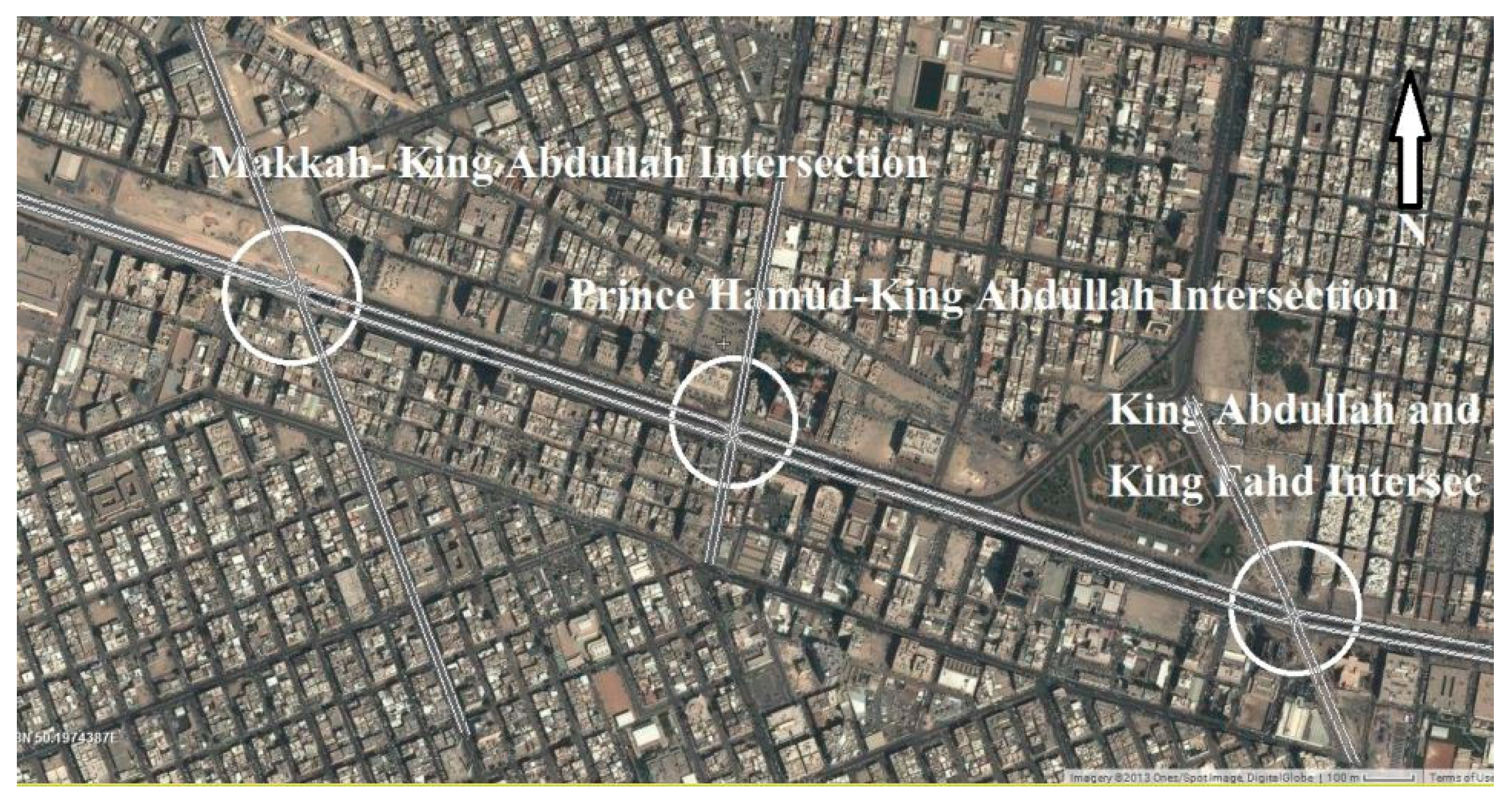
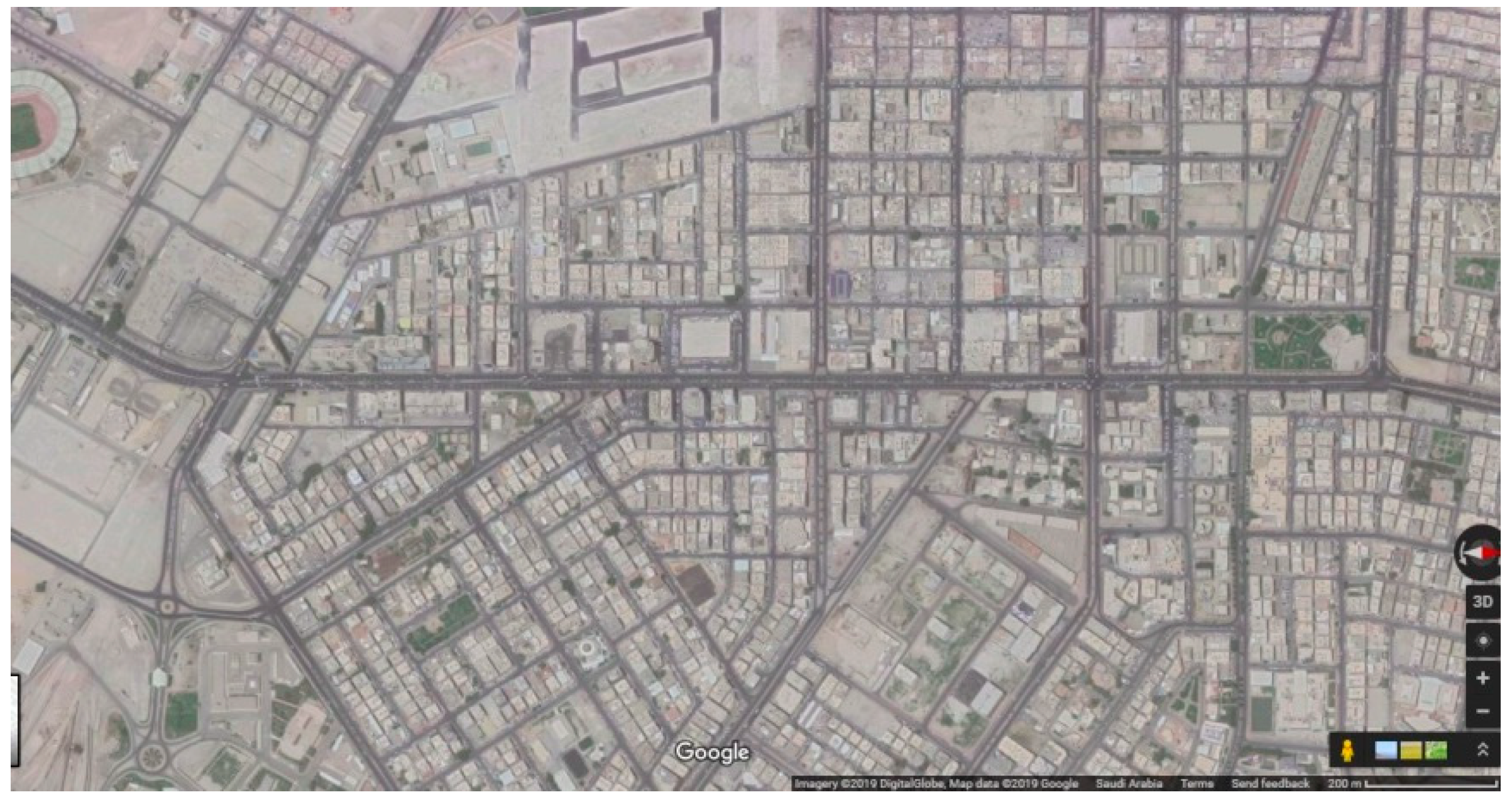
3. Study Area
4. Data Collection
5. Selection of Simulation Model
6. Selection of Calibration Parameters
7. Network Coding in VISSIM and Model Verification
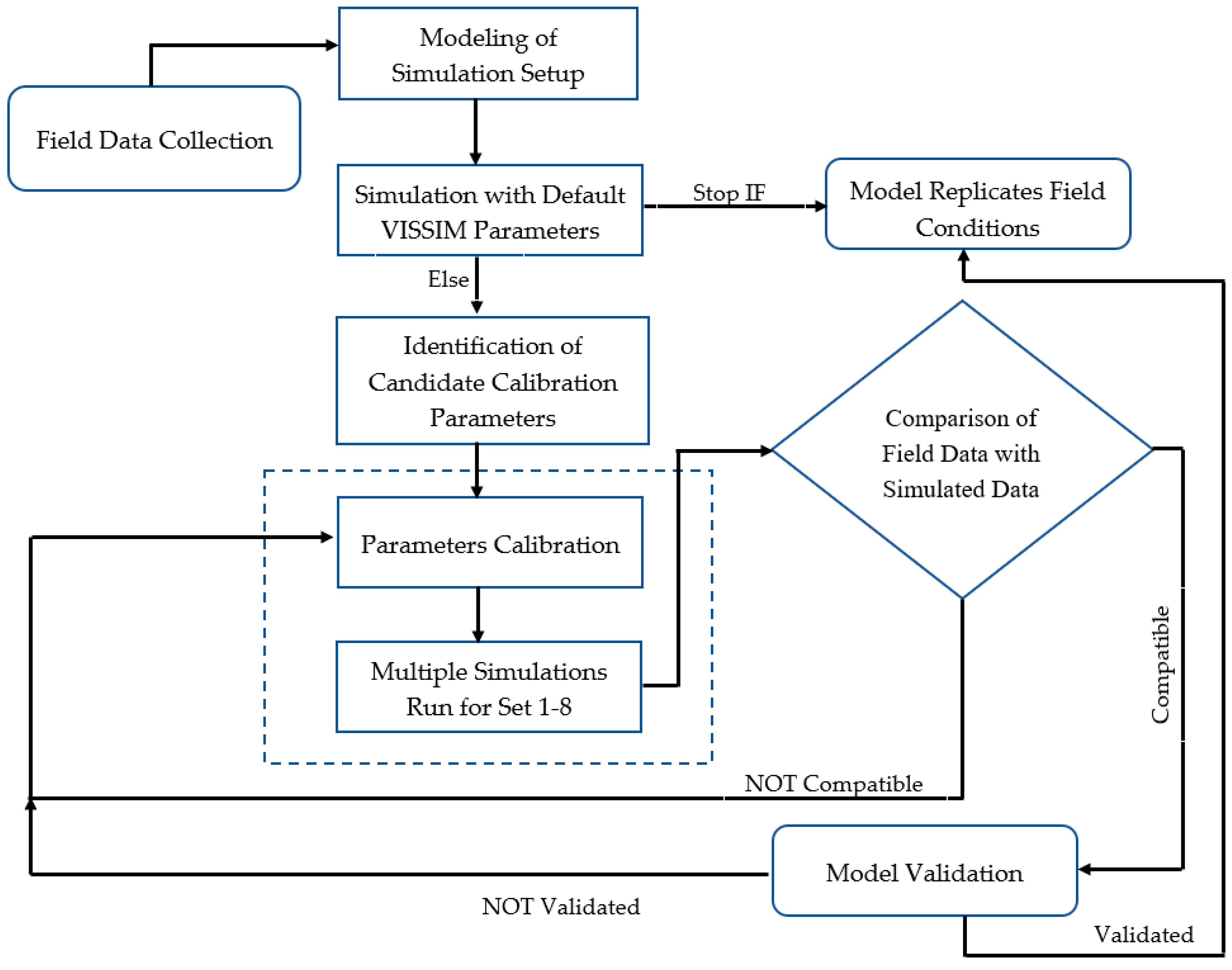
8. Calibration and Validation of VISSIM
8.1. Calibration Procedure
8.2. Results and Discussion
8.3. Model Validation
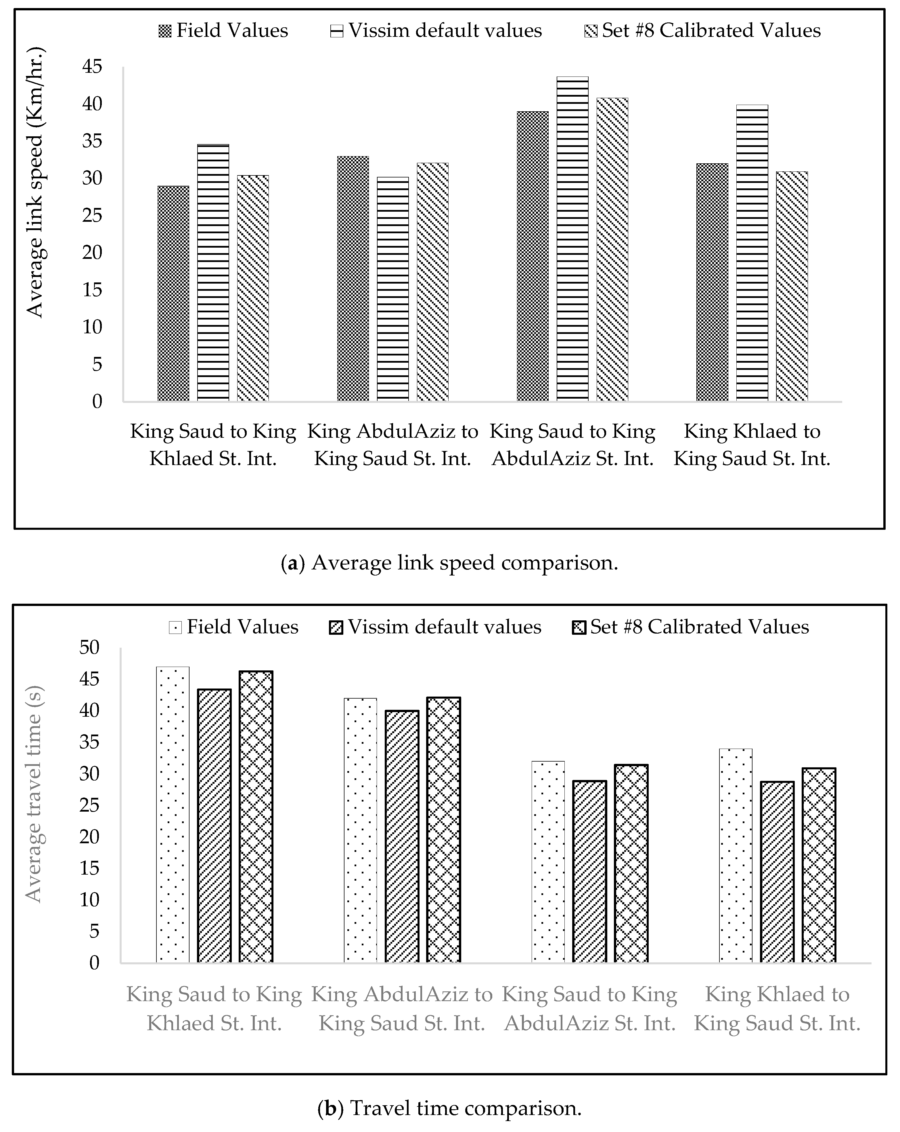
8.4. Comparison of Calibrated Driving Behavior Parameters
9. Conclusions
10. Study Limitations and Recommendations
Author Contributions
Funding
Acknowledgments
Conflicts of Interest
References
- Giuffrè, T.; Trubia, S.; Canale, A.; Persaud, B. Using microsimulation to evaluate safety and operational implications of newer roundabout layouts for European Road networks. Sustainability 2017, 9, 2084. [Google Scholar] [CrossRef]
- Young, W.; Sobhani, A.; Lenné, M.G.; Sarvi, M. Simulation of safety: A review of the state of the art in road safety simulation modelling. Accid. Anal. Prev. 2014, 66, 89–103. [Google Scholar] [CrossRef] [PubMed]
- Chen, C.; Zhao, X.; Liu, H.; Ren, G.; Zhang, Y.; Liu, X. Assessing the Influence of Adverse Weather on Traffic Flow Characteristics Using a Driving Simulator and VISSIM. Sustainability 2019, 11, 830. [Google Scholar] [CrossRef]
- Astarita, V.; Giofré, V.; Guido, G.; Vitale, A. Calibration of a new microsimulation package for the evaluation of traffic safety performances. Procedia-Soc. Behav. Sci. 2012, 54, 1019–1026. [Google Scholar] [CrossRef]
- Mahmud, S.S.; Ferreira, L.; Hoque, M.S.; Tavassoli, A. Micro-simulation modelling for traffic safety: A review and potential application to heterogeneous traffic environment. IATSS Res. 2018, 43, 27–36. [Google Scholar] [CrossRef]
- Lu, Z.; Fu, T.; Fu, L.; Shiravi, S.; Jiang, C. A video-based approach to calibrating car-following parameters in VISSIM for urban traffic. Int. J. Transp. Sci. Technol. 2016, 5, 1–9. [Google Scholar] [CrossRef] [Green Version]
- Espejel-Garcia, D.; Saniger-Alba, J.A.; Wenglas-Lara, G.; Espejel-Garcia, V.V.; Villalobos-Aragon, A. A Comparison among Manual and Automatic Calibration Methods in VISSIM in an Expressway (Chihuahua, Mexico). Open J. Civ. Eng. 2017, 7, 539–552. [Google Scholar] [CrossRef] [Green Version]
- Fellendorf, M.; Vortisch, P. Fundamentals of Traffic Simulation; Springer: New York, NY, USA, 2010; Volume 145. [Google Scholar]
- Henclewood, D.; Suh, W.; Rodgers, M.O.; Fujimoto, R.; Hunter, M.P. A calibration procedure for increasing the accuracy of microscopic traffic simulation models. Simulation 2017, 93, 35–47. [Google Scholar] [CrossRef]
- Manjunatha, P.; Vortisch, P.; Mathew, T. Methodology for the Calibration of VISSIM in Mixed Traffic. Transportation Research Board 92nd Annual Meeting. 2013. Available online: http://docs.trb.org/prp/13-3677.pdf (accessed on 12 March 2019).
- Mehar, A.; Chandra, S.; Velmurugan, S. Highway capacity through vissim calibrated for mixed traffic conditions. KSCE J. Civ. Eng. 2014, 18, 639–645. [Google Scholar] [CrossRef]
- Park, B.; Schneeberger, J.D. Microscopic simulation model calibration and validation: Case study of VISSIM simulation model for a coordinated actuated signal system. Transp. Res. Rec. 2003, 1856, 185–192. [Google Scholar] [CrossRef]
- Song, R.; Sun, J. Calibration of a micro-traffic simulation model with respect to the spatial-temporal evolution of expressway on-ramp bottlenecks. Simulation 2016, 92, 535–546. [Google Scholar] [CrossRef]
- Srikanth, S.; Mehar, A.; Parihar, A. Calibration of Vissim Model for Multilane Highways Using Speed Flow Curves. Stavební Obz. Civ. Eng. J. 2017, 26, 303–314. [Google Scholar] [CrossRef]
- Bonsall, P.; Liu, R.; Young, W. Modelling safety-related driving behaviour—impact of parameter values. Transp. Res. Part A Policy Pract. 2005, 39, 425–444. [Google Scholar] [CrossRef]
- Yu, M.; Fan, W.D. Calibration of microscopic traffic simulation models using metaheuristic algorithms. Int. J. Transp. Sci. Technol. 2017, 6, 63–77. [Google Scholar] [CrossRef]
- Jing, D.; Andrew, H.; Navid, S.; Chaoru, L.; Neal, H. VISSIM Calibration for Urban Freeways ISU Non-Discrimination Statement Iowa DOT Statements; Iowa State University: Ames, IA, USA, 2015. [Google Scholar]
- Sacks, J.; Rouphail, N.; Park, B.; Thakuriah, P. Statistically-based validation of computer simulation models in traffic operations and management. J. Transp. Stat. 2002, 5, 1–24. Available online: http://www.academia.edu/download/30900159/JTSStatisticalCORSIMWithDiscussion.pdf (accessed on 19 February 2019).
- Siddharth, S.P.; Ramadurai, G. Calibration of VISSIM for Indian heterogeneous traffic conditions. Procedia-Soc. Behav. Sci. 2013, 104, 380–389. [Google Scholar] [CrossRef]
- Mathew, T.V.; Radhakrishnan, P. Calibration of microsimulation models for nonlane-based heterogeneous traffic at signalized intersections. J. Urban Plan. Dev. 2010, 136, 59–66. [Google Scholar] [CrossRef]
- Nomani Kabir, M.; Alginahi, Y.M.; Mohamed, A.I. Modeling and Simulation of Traffic Flow: A Case—First Ring Road in Downtown Madinah. Int. J. Softw. Eng. Comput. Syst. (IJSECS) 2016, 2289–8522. [Google Scholar] [CrossRef]
- Ratrout, N.T.; Rahman, S.M.; Reza, I. Calibration of PARAMICS Model: Application of Artificial Intelligence-Based Approach. Arab. J. Sci. Eng. 2015, 40, 3459–3468. [Google Scholar] [CrossRef]
- Reza, I.; Ratrout, N.; Rahman, S.M. Calibration protocol for PARAMICS microscopic traffic simulation model: Application of neuro-fuzzy approach. Can. J. Civ. Eng. 2007, 43, 361–368. [Google Scholar] [CrossRef]
- Yang, Y.; Qin, Y.; Dong, H.; Zhang, Q. Parameter Calibration Method of Microscopic Traffic Flow Simulation Models based on Orthogonal Genetic Algorithm. In Proceedings of the 22nd International Conference on Distributed Multimedia Systems, Salerno, Italy, 25–26 November 2016; pp. 55–60. [Google Scholar] [CrossRef]
- Menneni, S.; Sun, C.; Vortisch, P. Microsimulation calibration using speed-flow relationships. Transp. Res. Rec. 2008, 2088, 1–9. [Google Scholar] [CrossRef]
- Wiedemann, R. Simulation des Strassenverkehrsflusses; Schriftenreihe des Instituts für Verkehrswesen der Universität Karlsruhe: Karlsruhe, Germany, 1974. [Google Scholar]
- Wiedemann, R. Modelling of RTI-Elements on multi-lane roads. In Advanced Telematics in Road Transport, Proceedings of the DRIVE Conference. Volume II; Elsevier: New York, NY, USA, 1991. [Google Scholar]
- Shaaban, K.; Kim, I. Comparison of SimTraffic and VISSIM microscopic traffic simulation tools in modeling roundabouts. Procedia Comput. Sci. 2015, 52, 43–50. [Google Scholar] [CrossRef]
- Uludamar, E.; Tuccar, G. Comparison of Traffic Densities at Different Signalization Timings in Roundabouts. J. Eng. Sci. 2018, 7, 217–223. [Google Scholar] [CrossRef]
- Ciuffo, B.; Punzo, V.; Torrieri, V. Comparison of simulation-based and model-based calibrations of traffic-flow microsimulation models. Transp. Res. Rec. 2008, 2088, 36–44. [Google Scholar] [CrossRef]
- Ma, J.; Dong, H.; Zhang, H.M. Calibration of microsimulation with heuristic optimization methods. Transp. Res. Rec. 2007, 1999, 208–217. [Google Scholar] [CrossRef]
- Hourdakis, J.; Michalopoulos, P.G.; Kottommannil, J. Practical procedure for calibrating microscopic traffic simulation models. Transp. Res. Rec. 2003, 1852, 130–139. [Google Scholar] [CrossRef]
- Lee, J.B.; Ozbay, K. New calibration methodology for microscopic traffic simulation using enhanced simultaneous perturbation stochastic approximation approach. Transp. Res. Rec. 2009, 2124, 233–240. [Google Scholar] [CrossRef]
- Balakrishna, R.; Antoniou, C.; Ben-Akiva, M.; Koutsopoulos, H.N.; Wen, Y. Calibration of microscopic traffic simulation models: Methods and application. Transp. Res. Rec. 2007, 1999, 198–207. [Google Scholar] [CrossRef]
- Abdalhaq, B.K.; Baker, M.I. Using meta heuristic algorithm to improve traffic simulation. J. Algorithm Optim. 2014, 2, 110–128. [Google Scholar]
- Kim, S.J.; Kim, W.; Rilett, L.R. Calibration of microsimulation models using nonparametric statistical techniques. Transp. Res. Rec. 2005, 1935, 111–119. [Google Scholar] [CrossRef]
- Asamer, J.; van Zuylen, H.J.; Heilmann, B. Calibrating VISSIM to adverse weather conditions. In Proceedings of the 2nd International Conference on Models and Technologies for Intelligent Transportation Systems, Leuven, Belgium, 22–24 June 2011; Volume 22, p. 24. [Google Scholar]
- Zhizhou, W.; Jian, S.; Xiaoguang, Y. Calibration of VISSIM for shanghai expressway using genetic algorithm. In Proceedings of the IEEE Winter Simulation Conference, Orlando, FL, USA, 4 December 2005; p. 4. [Google Scholar]
- Park, B.; Qi, H. Development and Evaluation of a Procedure for the Calibration of Simulation Models. Transp. Res. Rec. J. Transp. Res. Board 2005, 208–217. [Google Scholar] [CrossRef]
- Punzo, V.; Ciuffo, B. How parameters of microscopic traffic flow models relate to traffic conditions and implications on model calibration. Transp. Res. Rec. J. Transp. Res. Board 2009, 2124, 249–256. [Google Scholar] [CrossRef]
- Ge, Q.; Menendez, M. Sensitivity Analysis for Calibrating VISSIM in Modeling the Zurich Network. In Proceedings of the 12th Swiss Transport Research Conference, Ascona, Switzerland, 2–4 May 2012. [Google Scholar]
- Chu, L.; Liu, H.X.; Oh, J.S.; Recker, W. A calibration procedure for microscopic traffic simulation. In Proceedings of the 2003 IEEE International Conference on Intelligent Transportation Systems, Shanghai, China, 12–15 October 2003; Volume 2, pp. 1574–1579. [Google Scholar] [CrossRef]
- Oregon Department of Transportation. Protocol for VISSIM Simulation; Oregon Department of Transportation: Salem, OR, USA, 2011.
- Washington State Department of Transportation. Protocol for VISSIM Simulation; Washington State Department of Transportation: Olympia, WA, USA, 2014.
- Maryland Department of Transportation. VISSIM Modeling Guidance; Maryland Department of Transportation: Hanover, MD, USA, 2017.
- Fred, C.; Milam, R.T.; David, S. CORSIM, PARAMICS, and VISSIM: What the Manuals Never Told You. In Proceedings of the Ninth TRB Conference on the Application of Transportation Planning Methods, Baton Rouge, LA, USA, 6–10 April 2003. [Google Scholar]
- Park, B.; Won, J.; Yun, I. Application of microscopic simulation model calibration and validation procedure: Case study of coordinated actuated signal system. Transp. Res. Rec. 2006, 1978, 113–122. [Google Scholar] [CrossRef]


| Authors | Microsimulation Used | Calibration Parameters |
|---|---|---|
| Ciuffo et al. [30] | AIMSUN | Drivers’ reaction time and speed acceptance |
| Ma et al. [31] | PARAMICS | Mean reaction time and mean headway |
| Mennini et al. [25] | VISSIM | CC1, CC2, CC3, CC4, CC5 (Wiedemen co-efficient) |
| Hourdakis et al. [32] | AIMSUN | Max. acc. rate, max speed diff., avg. speed, and 9 other parameters |
| Lee and Ozbay [33] | PARAMICS | Mean reaction time and mean headway |
| Balakrishna et al. [34] | MITSimLab | Car following and lane changing co-efficients |
| Abdalhaq and Baker [35] | SUMO | Deceleration, acceleration, and driver imperfections, etc. |
| Kim et al. [36] | VISSIM | Number of observed preceding vehicles, look-ahead distance, average standstill distance, Additive parameter and a multiplicative parameter and lane change distance |
| Parameter Description | VISSIM Default Values |
|---|---|
| Lane change distance (m) | 200 m |
| No. of preceding observed vehicles | 2 |
| Amber signal decision model | Continuous Check |
| Additive part of safety distance (m) | 2 |
| Multiplicative Part of safety distance (m) | 3 |
| Minimum headway (s) | 0.5 |
| Parameters | Description | Validation Benchmark |
|---|---|---|
| Average travel speed | Standard deviation for individual links is within simulated average travel speed and floating car average travel speed | Within 1 Standard Deviation (SD) |
| Average travel time | Standard deviation for series of links is within simulated average travel time and floating car average travel time | Within 1 Standard Deviation (SD) |
| Maximum and average queue length | Percent difference in simulated and observed queue lengths | 80–120% of actual observed value |
| Parameters | Parameter Values VISSIM Default | Calibrated Parameter Values | |||||||
|---|---|---|---|---|---|---|---|---|---|
| Set#1 | Set#2 | Set#3 | Set#4 | Set#5 | Set#6 | Set#7 | Set#8 | ||
| Lane change distance (m) | 200 | 300 | 300 | 300 | 250 | 250 | 250 | 200 | 200 * |
| No. of preceding Observed vehicles | 2 | 2.25 | 2.50 | 2.75 | 3.0 | 3.5 | 3.5 | 3.75 | 4 * |
| Additive part of safety- distance | 2 | 2.10 | 2.10 | 2.15 | 2.20 | 2.20 | 2.25 | 2.25 | 2.25 * |
| Multiplicative part of safety distance | 3 | 3.15 | 3.15 | 3.15 | 3.20 | 3.25 | 3.25 | 3.25 | 3.25 * |
| Minimum headway | 0.5 | 1.0 | 1.0 | 1.0 | 1.5 | 1.5 | 1.5 | 1.75 | 1.75 |
| Amber signal decision model | Continuous check | One decision | One decision | Continuous check | One decision | Continuous check | Continuous check | One decision | Continuous check * |
| Route | Distance (m) | Field Values | SD | VISSIM Default (within 1 SD) | Calibrated Travel Time (s) (All Sets are within 1 SD Range) | |||||||
|---|---|---|---|---|---|---|---|---|---|---|---|---|
| Set#1 | Set#2 | Set#3 | Set#4 | Set#5 | Set#6 | Set#7 | Set#8 | |||||
| Hamoud St. Int. to Macca St. Int. | 750 | 55 | 3.79 | 49.57 (NO) | 50.86 (NO) | 49.48 (NO) | 49.49 (NO) | 49.86 (NO) | 49.94 (NO) | 50.9 (NO) | 51.13 (NO) | 51.2 (YES) |
| Hamoud St. Int. to Abdul Aziz St. Int. | 985 | 68 | 4.77 | 62.21 (NO) | 62.42 (NO) | 61.7 (NO) | 61.8 (NO) | 62.48 (NO) | 62.44 (NO) | 62.55 (NO) | 63.01 (NO) | 63.4 (YES) |
| Macca St. Int. to Hamoud St. Int. | 735 | 59 | 4.56 | 54.12 (NO) | 54.9 (YES) | 53.88 (NO) | 54.99 (YES) | 54.20 (NO) | 55 (YES) | 55.29 (YES) | 55.44 (YES) | 56.1 (YES) |
| Macca St. Int. to Ab. Aziz St. Int. | 1873.5 | 188 | 4.69 | 183 (NO) | 182.8 (NO) | 181.6 (NO) | 182.9 (NO) | 182.37 (NO) | 183.9 (YES) | 184.5 (YES) | 183.9 (YES) | 185 (YES) |
| Ab. Aziz St. Int. to Macca St. Int. | 1898.2 | 168 | 5.02 | 162.16 (NO) | 164.3 (YES) | 162.7 (NO) | 162.7 (NO) | 162.70 (NO) | 162.9 (NO) | 164.4 (YES) | 164.4 (YES) | 165 ((YES) |
| Abdul Aziz St. Int. to Hamoud St. Int. | 1000 | 73 | 3.74 | 68.78 (NO) | 69.87 (YES) | 68.97 (NO) | 69 (NO) | 68.94 (NO) | 69 (NO) | 69.79 (YES) | 69.85 (YES) | 69.8 (YES) |
| Route | Distance (m) | Field Values | SD | VISSIM Default (within 1 SD) | Calibrated Average Speed (km/h) (All sets are within 1 SD range) | |||||||
|---|---|---|---|---|---|---|---|---|---|---|---|---|
| Set#1 | Set#2 | Set#3 | Set#4 | Set#5 | Set#6 | Set#7 | Set#8 | |||||
| Macca St. Int. to Hamoud St. Int. | 735 | 46.2 | 2.93 | 50.21 (NO) | 49.48 (NO) | 50.39 (NO) | 49.59 (NO) | 50.14 (NO) | 49.6 (NO) | 48.83 (YES) | 49.14 (NO) | 48.67 (YES) |
| Abdul-Aziz St. Int. to Hamoud St Int | 1000 | 50.15 | 2.4 | 52.73 (NO) | 51.92 (YES) | 52.55 (NO) | 52.54 (YES) | 52.55 (YES) | 52.5 (YES) | 51.98 (YES) | 51.93 (YES) | 51.95 (YES) |
| Hamoud St. Int. to Abdul-Aziz St. Int. | 985 | 52.15 | 3.06 | 56.09 (NO) | 55.87 (NO) | 56.44 (NO) | 56.42 (NO) | 55.81 (NO) | 55.8 (NO) | 55.76 (NO) | 55.46 (NO) | 55.14 (YES) |
| Hamoud St. Int. to Macca St. Int. | 750 | 57.45 | 2.66 | 54.51 (NO) | 53.46 (NO) | 54.61 (NO) | 54.62 (NO) | 54.24 (NO) | 54.2 (NO) | 53.38 (NO) | 53.12 (NO) | 53.1 (YES) |
| Intersection | Approach From | Queue Length Field (m) | Queue Length VISSIM Default (m) | Calibrated Maximum Queue Length (m) (% Variance is within the Range of 80–120% of Field Value) | ||||||||||||||||
|---|---|---|---|---|---|---|---|---|---|---|---|---|---|---|---|---|---|---|---|---|
| QL | % Var | Set#1 | Set#2 | Set#3 | Set#4 | Set#5 | Set#6 | Set#7 | Set#8 | |||||||||||
| QL | % Var | QL | % Var | QL | % Var | QL | % Var | QL | % Var | QL | % Var | QL | % Var | QL | % Var | |||||
| Abdul Aziz St. Int. | Dhahran | 39.2 | 40.8 | −4.1 (YES) | 40.1 | −2.3 (YES) | 41.1 | −4.8 (YES) | 41.5 | −5.9 (YES) | 40.5 | −3.3 (YES) | 40.9 | −4.3 (YES) | 40.7 | −3.8 (YES) | 39.8 | −1.5 (YES) | 39.9 | −1.8 (YES) |
| Abdul Aziz St. Int. | Khobar | 32.7 | 27.5 | 15.9 (YES) | 27.6 | 15.6 (YES) | 27.6 | 15.6 (YES) | 28.1 | 14.1 (YES) | 27.8 | 15.0 (YES) | 28.4 | 13.2 (YES) | 27.9 | 14.7 (YES) | 27.6 | 15.6 (YES) | 28 | 14.3 (YES) |
| Hamoud St. Int. | Dhahran | 52.7 | 58.8 | −11.6 (NO) | 57.3 | −8.7 (NO) | 58.4 | −10.9 (NO) | 60 | −13.9 (NO) | 58.4 | −10.8 (NO) | 60 | −13.9 (NO) | 58.8 | −11.6 (NO) | 57.9 | −9.9 (NO) | 58.8 | −11.6 (YES) |
| Hamoud St. Int. | Khobar | 31.5 | 33.8 | −7.3 (NO) | 32.9 | −4.4 (YES) | 34.2 | −8.6 (YES) | 34.4 | −9.2 (YES) | 34.2 | −8.6 (YES) | 34.2 | −8.6 (YES) | 33 | −4.8 (YES) | 32.7 | −3.8 (YES) | 32.7 | −3.8 (YES) |
| Macca St. Int. | Dhahran | 55.9 | 51.7 | 7.5 (YES) | 53 | 5.2 (NO) | 53.4 | 4.5 (YES) | 55.1 | 1.4 (YES) | 53.5 | 4.3 (YES) | 55.4 | 0.9 (YES) | 54.6 | 2.3 (YES) | 53.1 | 5.0 (YES) | 54.7 | 2.1 (YES) |
| Macca St. Int. | Khobar | 21.2 | 23.2 | −9.4 (NO) | 22 | −3.8 (NO) | 23.5 | −10.9 (NO) | 23.6 | −11.3 (NO) | 23.2 | −9.4 (YES) | 23.2 | −9.4 (YES) | 22.1 | −4.2 (YES) | 21.8 | −2.8 (YES) | 21.7 | −2.4 (YES) |
| Intersection | Approach From | Queue Length Field (m) | Queue Length VISSIM Default (m) | Calibrated Maximum Queue Length (m) (% Variance is within the Range of 80–120% of Field Value) | ||||||||||||||||
|---|---|---|---|---|---|---|---|---|---|---|---|---|---|---|---|---|---|---|---|---|
| QL | % Var | Set#1 | Set#2 | Set#3 | Set#4 | Set#5 | Set#6 | Set#7 | Set#8 | |||||||||||
| QL | % Var | QL | % Var | QL | % Var | QL | % Var | QL | % Var | QL | % Var | QL | % Var | QL | % Var | |||||
| Abdul Aziz St. Int. | Dhahran | 45 | 58.8 | −30.7 (NO) | 56.4 | −25.3 (NO) | 54.5 | −21.11 (NO) | 50.2 | −11.56 (YES) | 55.5 | −23.33 (NO) | 49.2 | −9.3 (YES) | 44.5 | 1.11 (YES) | 43.6 | 3.11 (YES) | 44.9 | 0.22 (YES) |
| Abdul Aziz St. Int. | Khobar | 40.5 | 31.2 | 22.9 (NO) | 30.8 | 23.95 (NO) | 28.5 | 29.63 (NO) | 29.5 | 27.16 (NO) | 32.6 | 19.51 (YES) | 31.1 | 23.2 (NO) | 31.2 | 22.9 (NO) | 31.2 | 22.96 (NO) | 36.4 | 10.1 (YES) |
| Hamoud St. Int. | Dhahran | 63 | 76.5 | −21.4 (NO) | 78.5 | −24.6 (NO) | 78.5 | −24.6 (NO) | 75.8 | −20.32 (NO) | 70.4 | −11.75 (YES) | 78.4 | −24.4 (NO) | 62.1 | 1.43 (YES) | 63.2 | −0.32 (YES) | 66.4 | −5.4 (YES) |
| Hamoud St. Int. | Khobar | 36 | 44.3 | −23.1 (NO) | 45.5 | −26.4 (NO) | 42.4 | −17.78 (YES) | 40.1 | −11.39 (YES) | 42.8 | −18.89 (YES) | 43.8 | −21.7 (NO) | 34.8 | 3.33 (YES) | 34.8 | 3.33 (YES) | 36.2 | −0.56 (YES) |
| Macca St. Int. | Dhahran | 63 | 78.2 | −24.1 (NO) | 76.4 | −21.3 (NO) | 72.2 | −14.6 (YES) | 74.4 | −18.1 (YES) | 72.8 | −15.56 (YES) | 60.4 | 4.12 (YES) | 56.2 | 10.8 (YES) | 57.5 | 8.73 (YES) | 57.1 | 9.36 (YES) |
| Macca St. Int. | Khobar | 36 | 25.6 | 28.89 (NO) | 25.4 | 29.44 (NO) | 26.5 | 26.39 (NO) | 27.4 | 23.89 (NO) | 28.6 | 20.56 (NO) | 32.6 | 9.44 (YES) | 24.4 | 32.2 (NO) | 26.4 | 26.7 (NO) | 32.7 | 9.17 (YES) |
| Street Name | Percentage Difference in Average Aped (kmph) | Percentage Difference in Travel Time (sec) | Percentage Difference in Average Queue (m) | Percentage Difference in Maximum Queue (m) | ||||
|---|---|---|---|---|---|---|---|---|
| VISSIM Default | Set #8 | VISSIM Default | Set #8 | VISSIM Default | Set #8 | VISSIM Default | Set #8 | |
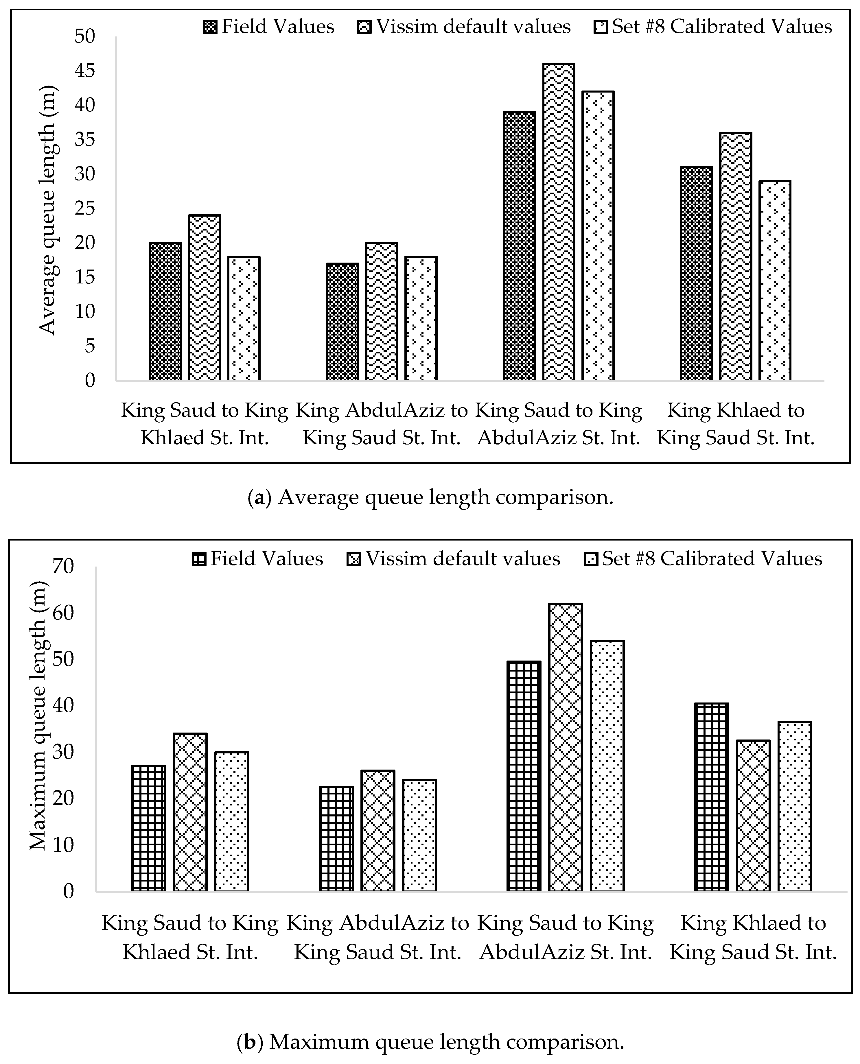
| King Saud to King Khaled St. Int. | 19.31 | 4.90 | −7.66 | −1.55 | 20.00 | −8.80 | 25.93 | 9.67 |
| King Abdul-Aziz to King Saud St. Int. | −8.48 | −2.73 | −4.76 | 0.29 | 17.65 | 5.88 | 15.56 | 6.67 |
| King Saud to King Abdul-Aziz St. Int. | 12.00 | 4.72 | −9.69 | −1.81 | 17.95 | 7.69 | 25.25 | 9.09 |
| King Khaled to King Saud St. Int. | 24.69 | −3.31 | −15.29 | −9.12 | 16.13 | −6.45 | −19.75 | −9.88 |
| Calibration Parameters | Default Value | Siddharth and Ramaduraib [19] | Park and Schneeberger [14] | Yu et al. [16] | Park et al. [47] | Park and Qi [39] | This Study |
|---|---|---|---|---|---|---|---|
| Minimum headway (front/rear) | 0.5 | 0.11 | 3.0 | 1.0 | 1.75 | - | 1.75 |
| Average standstill distance CC0 | 2.0 | 1.0 | 3.0 | 1.6 | 1.73 | 3.85 | - |
| Additive part of safety distance | 2.0 | 0.20 | - | 4.40 | 1.08 | 5.0 | 2.25 |
| Multiplicative part of safety distance | 3.0 | 0.78 | - | 3.72 | 2.57 | 5.3 | 3.25 |
| Lane change distance (m) | - | 175 | - | - | - | 200 | |
| No. of observed Vehicles | 2.0 | - | 4.0 | - | - | 4.0 | 4.0 |
| Waiting time before diffusion (s) | 60 | - | 60 | 64.2 | 32.73 | - | - |
© 2019 by the authors. Licensee MDPI, Basel, Switzerland. This article is an open access article distributed under the terms and conditions of the Creative Commons Attribution (CC BY) license (http://creativecommons.org/licenses/by/4.0/).
Share and Cite
Al-Ahmadi, H.M.; Jamal, A.; Reza, I.; Assi, K.J.; Ahmed, S.A. Using Microscopic Simulation-Based Analysis to Model Driving Behavior: A Case Study of Khobar-Dammam in Saudi Arabia. Sustainability 2019, 11, 3018. https://0-doi-org.brum.beds.ac.uk/10.3390/su11113018
Al-Ahmadi HM, Jamal A, Reza I, Assi KJ, Ahmed SA. Using Microscopic Simulation-Based Analysis to Model Driving Behavior: A Case Study of Khobar-Dammam in Saudi Arabia. Sustainability. 2019; 11(11):3018. https://0-doi-org.brum.beds.ac.uk/10.3390/su11113018
Chicago/Turabian StyleAl-Ahmadi, Hassan M., Arshad Jamal, Imran Reza, Khaled J. Assi, and Syed Anees Ahmed. 2019. "Using Microscopic Simulation-Based Analysis to Model Driving Behavior: A Case Study of Khobar-Dammam in Saudi Arabia" Sustainability 11, no. 11: 3018. https://0-doi-org.brum.beds.ac.uk/10.3390/su11113018