Assessment of Ecosystem Services Value Based on Land Use and Land Cover Changes in the Transboundary Karnali River Basin, Central Himalayas

Abstract

Land use and land cover change (LUCC) and its spatio-temporal characteristics are essential for natural resource management and sustainable development. LUCC is one of the major factors that affect the ecosystem and the services it provides. In this study, we used remote sensing techniques and a geographical information system to extract the land cover categories based on the Object-Based Image Analysis (OBIA) technique from Landsat TM/ETM/OLI satellite images in the transboundary Karnali River Basin (KRB, China and Nepal) of central Himalayas from 2000 to 2017. Spatio-temporal integrated methodology—Tupu was used to spatially show the LUCC as well as spatial characteristics of the arisen Tupu and shrunken Tupu. In addition, the ecosystem services value (ESV) were obtained and analyzed for each land cover category. In 2017, forest covered the highest area (33.45%) followed by bare area (30.3%), shrub/grassland (18.49%), agriculture (13.12%), snow/ice (4.32%), waterbody (0.3%) and built-up area (0.04%) in the KRB. From 2000 to 2017, the areas of forest, waterbody and snow/ice have decreased by 0.59, 6.14, and 1072.1 km², respectively. Meanwhile, the areas of shrub/grassland, agriculture, barren land, and built-up categories have increased by 82.21, 1.44, 991.97, and 3.11 km², respectively. These changes in the land cover have led to an increase in the ESV of the basin, especially the increase in shrub/grassland, agriculture, and water bodies (in the higher elevation). The total ESV of the basin was increased by $1.59 × 10⁶ from 2000 to 2017. Anthropogenic factors together with natural phenomena drive LUCC in the basin and thus the ESV. The findings of this study could facilitate the basin-level policy formulation to guide future conservation and development management interventions.

1. Introduction

Land use and land cover change (LUCC) significantly affect the major functioning aspects of the ecosystem [1] and are easily detectable indicators of changes in the global ecology [2,3,4,5,6,7]. Humans have been altering the earth’s surface at an alarming rate. The alteration in the land use and land cover (LULC) has a direct impact on biological diversity [8,9] as well as contributing to climate change at a different scale [10,11,12]. This leads to changes in the ecosystem services affecting the biological systems to support human needs [13]. These changes also partly determine the vulnerability of people and their dwelling places to climatic, economic or socio-political perturbations [14,15]. Thus, robust knowledge on LULC is fundamental to understand the landscape patterns and their changes—essential to assess the drivers and their impacts on the ecosystem services [16].

Ecosystem function refers to the habitat, biological or system properties and physical processes that occur within or across the ecosystem [17]. Ecosystem services are the benefits humans reap from the ecosystem function [17,18,19] that includes provisioning, regulating, cultural and supporting services [18,20]. In addition, the ecosystem function plays an important and multi-dimensional (ecological, socio-cultural and economic) role in the human society [21]. Ecosystem services do not directly flow from nature to human well-being, rather this occurs through the interaction with other forms of capital such as human capital (presence of human being), built capital (human built environment) and social capital (their community) [22]. Generally, the structure of the ecosystem is modified due to increased land use intensity and frequent changes in the land cover types. This results in changes in the ecosystem functions and the associated services it provides [23,24,25]. In recent decades, ecosystem services have been degrading due to an ever-increasing demand for these services, leading to a substantial and largely irreversible loss of natural and biological diversity life on earth [18]. The assessment and valuation of ecosystem services based on LUCC can be an important tool to raise awareness and convey the importance of ecosystem services [26]. Researchers have profoundly assessed the value of ecosystem services and studies have been conducted at the global scale [17,22] and regional scale (Tibetan Plateau, TP) [27], as well as at the national scale [28,29], to analyze the status, changes, and trends of ecosystem services [27,30,31,32,33]. During 1997–2011, the loss in global ecosystem services due to LUCC was estimated to be $4.3–20.2 trillion [22]. The annual ecological value of the TP was estimated to be $151 billion, accounting for 17.68% of China’s annual ecological value and 0.61% of the world [27]. Climate warming and local socio-economic development are the prime factors for the environmental–ecological system degradation of the TP [32].

The values of ecosystem services based on LUCC have recently been assessed for the transboundary Koshi river basin [28] and Gandaki river basin [29] of central Himalayas. However, to date, similar studies have not been conducted in the transboundary Karnali River Basin (KRB). Paudel et al. (2016) states that the 2010 global datasets of land cover are far from the reality and 2010 national datasets published by ICIMOD in 2015 [34] are closer to ground truth in Nepal. In this study, we aim to present the latest remote sensing-based land cover statistics of KRB and compare them with those of the global and national land cover database. Furthermore, we trace the LUCC from 2000 and assess the ecosystem services value (ESV) in the KRB. The spatio-temporal integrated landscape information Tupu methodology was put forward and adopted to assess LUCC. The landscape information Tupu provides the integrated spatial pattern and temporal processes of LUCC units [35]. Percentage-wise land cover statistics are compared among the three major river basins in Nepal. In addition, district-wise LULC statistics and possible driving factors for the land cover changes within the basin are discussed. The quantification of the ESV for different land cover categories in KRB has been assessed according to the coefficients of each land cover on ecosystem services adopted for the TP.

2. Materials and Methods

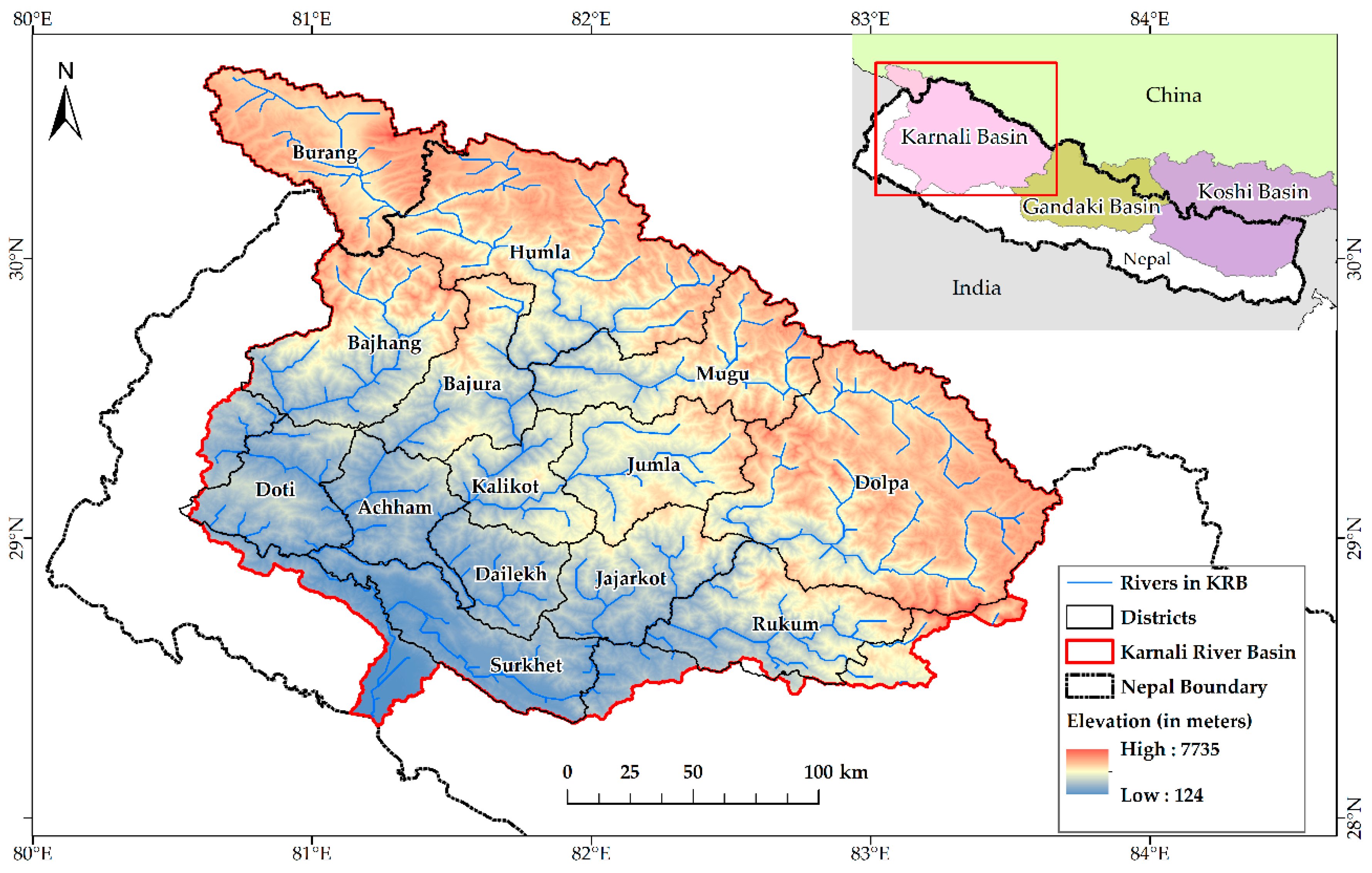
2.1. Study Area

The Karnali river basin (KRB) is one of the three major river basins in Nepal, the Gandaki and Koshi river basins being the other two (Figure 1). KRB is located in the western region of Nepal. The Karnali river that originates from the south of Mansarovar and Rokas lakes in China (Tibet) is the longest river flowing through Nepal, with many snow-fed rivers as its tributaries. This study focused on the transboundary KRB (China and Nepal) which extends from 28°19′39.44″ to 30°41′18.66″ N in latitude and 80°33′34.93″ to 83°40′55.74″ E in longitude. The KRB covers a total area of 46,124 km² with 3085 km² in China. With high variation in topography and elevation, the KRB covers all the five physiographic regions in Nepal, i.e., Terai (60–200 m), Siwalik (200–1300 m), Middle Mountain (1300–2700 m), High Mountain (2700–4000 m) and High Himalayas (>4000 m) [36]. Hence, all five climate zones exist in the basin that includes tropical, sub-tropical, temperate, sub-alpine and alpine climate zones. The climate of the KRB is influenced by South Asian Monsoon in the summer and westerlies in the winter season [37]. The average maximum and minimum temperature are 25 °C and 13 °C, respectively, with an average annual precipitation of 1479 mm. The temperature shows an increasing trend (by 0.05 °C per year for the maximum temperature and 0.01 °C per year for the minimum temperature), whereas the precipitation is in a decreasing trend by 4.91 mm per year in the KRB [38].

2.2. Data Collection

We used a total of 15 scenes of geometrically corrected Landsat Level 1 products that were downloaded from the United States Geological Survey’s (USGS) web portal. The details are shown in

Table 1. Landsat data used for the study.

Acquired Year	Number of Scenes	Sensor	Spatial Resolution (m)	Repeat Cycle (Days)	Number of Bands
2000	5	Enhanced Thematic Mapper (ETM)	30	16	6
2010	5	Thematic Mapper (TM)	30	16	6
2017	5	Operational Land Imager (OLI)	30	16	9

. The acquired Landsat images were of the post-monsoon period (October to early December) since this period is less affected by seasonal snow and cloud cover [39] and, the vegetation is mostly green to semi-deciduous [36]. Imageries of alternative years (±1 year) were used when good quality images (cloud and seasonal snow free) for a particular year were not available for improving classification accuracy. In some cases, the imageries from different seasons were used to check the best suitable images for classification.

Other datasets used were the national land cover data of 2010 developed by ICIMOD, which was downloaded from their website (http://rds.icimod.org/). The 30-m global land cover dataset of the year 2000 and 2010 produced by the National Geomatics Center of China was downloaded from their website (www.globallandcover.com). Other necessary auxiliary spatial datasets were collected from the Survey Department, Government of Nepal, which was basically used for the verification and validation of classification. The Shuttle Radar Topography Mission (SRTM) 30-m Digital Elevation Model (DEM) [40] was downloaded from the National Aeronautics and Space Administration’s (NASA) web portal (https://urs.earthdata.nasa.gov/).

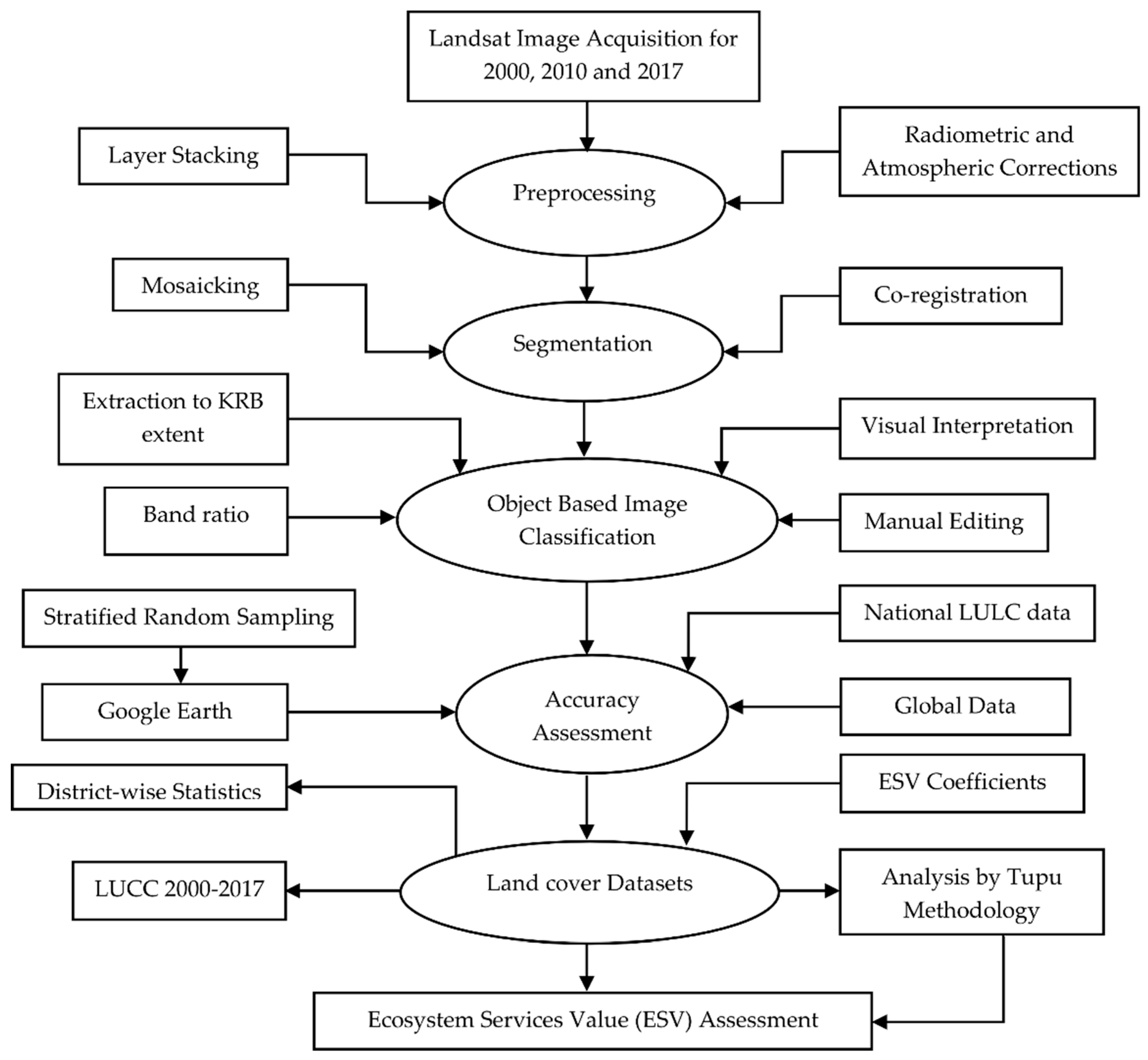
2.3. Image Pre-Processing and Classification

Different Landsat sensors have different bands and the bands were carefully stacked into one image using ENVI 5.3 software. Band composition is very crucial to carry out image classification (For Landsat 8, R, G, B: 5, 4, 3; for Landsat 5 and Landsat 7, R, G, B: 4, 3, 2). The Landsat images for the years 2000 and 2010 were clipped out to remove the colored lines at the edges of the images. Radiometric Calibration (Digital Number (DN) to top-of-atmosphere (TOA)) and atmospheric corrections (i.e., dark object subtraction) were applied to all the images. Images of the same study year were mosaicked to obtain a single image for the years 2000, 2010 and 2017, respectively. These images were co-registered for producing the change detection maps between different time periods, taking the 2017 image as baseline. The overall process followed in the study is shown in Figure 2.

The classification was carried out using the object-based image analysis (OBIA) in the eCognition Developer 9.0 software. OBIA gives better classification results with higher accuracy than the pixel-based methods because it uses spectral as well spatial information [16,41,42,43,44], which includes information such as texture, neighborhood, context and related ancillary data [45,46,47]. Meanwhile, SRTM DEM (30 m) was used to reduce the misclassification by removing the mountain shadow following the same procedure mentioned in a previous study [39]. The “multi-resolution segmentation” algorithm was used for the segmentation of the images, which clusters pixels into image objects based on their neighbors and relative homogeneity criteria [48,49,50]. Image layer weights of 1, scale parameter of 20, shape of 0.1, and compactness of 0.5 were used in the multiresolution segmentation algorithm. Multi-resolution segmentation is based on the assumption that similar features have similar spectral responses and the spectral response of an element would be unique concerning other aspects of interest [50].

The segmented objects were further processed and analyzed using different indices. The spectral values of the image layers were used to generate the image indices such as the normalized difference vegetation index (NDVI), normalized difference water index (NDWI), bare soil index (BSI) and normalized difference snow index (NDSI) derived through band rationing. The rules were set up for the image objects according to their attributes such as NDVI, NDWI, BSI, and NDSI layer values. Here, the image objects representing patterns are determined either by ground truth information or by comparing with high-resolution Google Earth images. Land cover data were extracted by classifying the image objects based on the rulesets developed by exploring the spectral bands and indices. Seven types of land cover categories were classified for the KRB. We used previous national [36] and global [51] datasets as well as Google Earth to validate and cross-check our classification output. The seven land cover classes were set up for the KRB, namely, Forest (1), Shrub/grassland (2), Agriculture (3), Bare area (4), Waterbody (5), Snow/Ice (6) and Built-up (7).

2.4. Accuracy Assessment

Accuracy assessment/validation of the results obtained from remotely sensed data is a necessity to know its quality [52,53]. The classification accuracy was assessed using user’s and producer’s accuracy, an error matrix and kappa coefficient [53]. The user’s accuracy measures error of commission—representing the likelihood of a classified pixel matching the ground reality. The producer’s accuracy measures error of omission—measuring how well the ground land cover types can be classified. The overall accuracy compares each classified pixel against the land cover obtained from corresponding ground truth [52,53]. Kappa statistics are used as a measure of agreement between reality and derived results [52] and were calculated using the equation that has been widely used in the previous LUCC studies [29,53,54]. The stratified random sampling method was used in this study to carry out the accuracy assessment of the classified data in Google Earth as well as in base imagery in ArcGIS. Google Earth is a freeware that provides high-resolution satellite imageries which act as an important reference for the validation of classification outputs [54] and has been widely used in many studies [29,36,55,56,57,58,59,60]. A total of 901, 905 and 890 stratified random points were generated in the classified image of 2000, 2010 and 2017, respectively, and were verified in Google Earth imageries. The topographical maps during 1992–2001 from the Survey Department, Government of Nepal were also used for data verification [29,59,61].

2.5. Spatio-Temporal Integrated Methodology—Tupu

Geo-information Tupu unit is the synthetic unit for geospatial-temporal analysis by “space-attribute-process” features and is composed of a relatively homogenous geographic and temporal unit, which was put forward by Ye et al. in 2004 [62]. When an integrated Tupu unit analysis is carried out, each geographical process of various events is synthesized into spatial and temporal attribute data [35]. Input and output are the two directions of land cover changes with regard to our starting set of attributes, the “reference” Tupu units. In the input diversion, also termed as the “arisen” series of Tupu units, other types of land cover are converted to the “reference” type. Similarly, in the output diversion, also termed as the “shrunken” series of Tupu units, the “reference” type of land cover diverts to other ones [62]. For example, when forest area is converted to agriculture, the arisen Tupu here is agriculture, whereas the shrunken Tupu is forest. We have evaluated the arisen and shrunken Tupu units from 2000 to 2017 and assessed the change in the value of ecosystem services. The detailed methodology described in the study carried out by Ye et al. [62] is used for calculation on Tupu units conversion.

2.6. Ecosystem Services Value Assessment

Costanza et al. [17] estimated the value per unit area of each ecosystem service for various ecosystems using the supply and demand analysis of the sum of consumer and producer surplus or the price times quantity for various ecological services. The 17 ecosystem services for 16 biomes were classified to estimate the global ESV. To derive the ESV coefficients, the values for ecosystem services per unit area by biome were estimated and then multiplied by the total area of each biome, which was summed over all services and biomes [17]. Various scholars have modified the global ESV coefficients [21,22,27]. Xie et al. [27] also updated and modified the coefficients of ESV for the TP based on Costanza’s global ESV. These modified coefficients of ESV were used in the assessment of ESV in the Koshi [28] and Gandaki river basins [29]. Since the physiographic as well as the climatic conditions of the KRB are similar to the other two basins in Nepal, the same modified coefficient values were used to estimate the ESV in the KRB (

Table 2. Land cover types and their ESV coefficients in Tibetan Plateau [27].

Land Cover Biome	ESV Coefficient ($ ha−1)
	2003	2010 *	2017 *
Forest	2168.84	2587.1	3017.23
Shrub land	1089.19	1299.24	1515.25
Grassland	565.88	675.01	787.24
Cropland	699.37	834.24	972.94
Barren area	59.83	71.37	83.23
Water bodies	6552.97	7816.72	9116.31
Snow/glacier	59.83	71.37	83.23

* Inflation-adjusted coefficient by using the Consumer Price Index (CPI) Inflation Calculator.

). In this study, the ESV coefficient for the category of shrub/grassland was calculated as the weighted average value between shrub and grassland. The ESV for the built-up category was not estimated due to the lack of coefficients values in the previous studies. Here, we adjusted the ESV coefficients of 2003 using the Consumer Price Index (CPI) Inflation Calculator obtained from the website of the Bureau of Labor Statistics, United States Department of Labor (https://www.bls.gov/data/inflation_calculator.htm) (Table 2).

The ESV for each land cover category was obtained by multiplying the area of each land cover with their individual coefficient (Table 2). Similarly, the ESV for each LC category that has changed was obtained in the form of arisen ESV and shrunken ESV. For instance, the arisen ESV of forest is assessed from the multiplication of the area of arisen forest Tupu with its respective ESV coefficient.

3. Results

3.1. Classification Accuracy Assessment

The user’s and producer’s accuracy for land cover classifications were calculated as 86.46 and 89.30% for 2017, 85.17 and 86.47% for 2010 and 83.83 and 85.72% for 2000, respectively. The overall accuracy was 89.4, 87.4 and 86.7% for the years 2017, 2010 and 2000, respectively. The kappa coefficients calculated were within the acceptable range of 0.87, 0.85 and 0.84 for the years 2017, 2010 and 2000, respectively [53]. The classification accuracy assessment in a confusion matrix for the year 2017 is given in

Table 3. User’s and producer’s accuracy assessment of the classification, 2017.

LULC Type	Forest	Shrub/Grassland	Agriculture	Bare Area	Waterbody	Snow/Ice	Built-Up	Total	User’s Accuracy	Producer’s Accuracy
Forest	185	8	3	2	0	0	0	198	93.43	94.87
Shrub/grassland	4	143	3	3	1	5	0	159	89.94	82.66
Agriculture	2	4	138	2	2	0	1	149	92.62	92.62
Bare Area	2	7	3	185	2	6	0	205	90.24	90.69
Waterbody	1	2	0	3	44	4	0	54	81.48	84.62
Snow/Ice	1	8	0	6	2	80	0	97	82.47	84.21
Built-up	0	1	2	3	1	0	21	28	75	95.45
Total	195	173	149	204	52	95	22	890

.

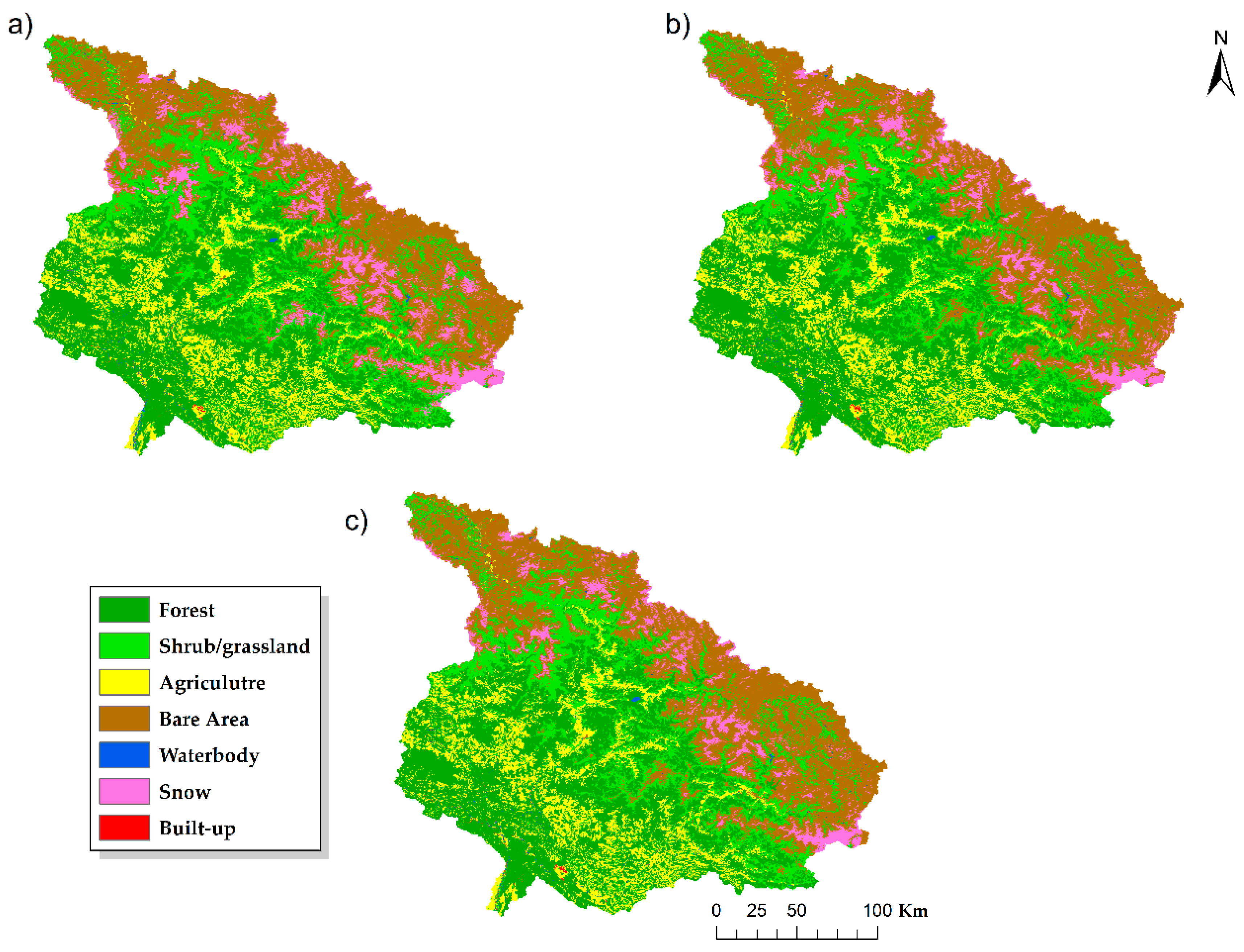
3.2. LC Statistics of the Basin

The KRB has been categorized into seven different LULC classes in 2000, 2010 and 2017 (Figure 3 and

Table 4. Land cover status in the KRB.

Land Cover Classes	Land Cover Area (km2)			Change from 2000–2017 (km2)
	2000	2010	2017
Forest	15,426.92	15,426.45	15,426.32	−0.59
Shrub/grassland	8445.37	8480.75	8527.58	82.21
Agriculture	6047.97	6103.79	6049.40	1.44
Bare Area	12,982.76	13,345.45	13,974.73	991.97
Waterbody	142.72	140.23	136.58	−6.14
Snow/Ice	3064.61	2610.55	1992.54	−1072.07
Built-up	13.45	16.50	16.57	3.11

). In 2017, forest covers the highest area (33.45%) in the basin, followed by bare area (30.3%), shrub/grassland (18.49%), agriculture (13.12%), snow/ice (4.32%), waterbody (0.3%) and built-up (0.04%). Similarly, in the year 2000, forest covers the highest area (33.45%), followed by bare area (28.15%), shrub/grassland (18.31%), agriculture (13.11%), snow/ice (6.64%), waterbody (0.31%) and built-up (0.03%). The result showed a slight decrease in the forest, waterbody and snow/ice categories in the datasets from 2000 to 2017. Meanwhile, the area of shrub/grassland, agriculture, bare area and built-up area have increased (Table 4).

3.3. LC Change from 2000 to 2017

The land cover of the Karnali basin has experienced subtle changes in the last 17 years. The result shows that 1.6 km² of forest area changed to agriculture. Similarly, the 2.9 km² change from agriculture was in the form of built-up (settlement) area due to human encroachment for settlements. The changes in the course of the river have led to 7 km² of bare area converting into the water bodies. The highest change in the entire basin was from snow to bare area by 997.6 km². Meanwhile, 70.7 km² of snow changed to shrub/grassland (

Table 5. Transition matrix of LUCC in the KRB from 2000 to 2017 (area km²).

2000	2017
	Forest	Shrub/Grassland	Agriculture	Bare	Waterbody	Snow	Built-Up
Forest	15,424.8	0.1	1.6	0.2	0.1	0	0
Shrub/grassland	0.3	8441.8	0.3	0.1	2.4	0	0
Agriculture	0.1	0.8	6043.7	0.3	0	0	2.9
Bare	0.1	7.8	0.2	12,967.1	7.0	0.1	0.3
Waterbody	0.3	6.0	3.2	8.6	123.2	0.9	0
Snow/ice	0	70.7	0.0	997.6	3.9	1991.1	0
Built-up	0	0	0.1	0	0	0	13.4

).

3.4. District-Wise LC Statistics

There are 13 districts in Nepal that completely lie inside the basin (Figure 1), while the China part is considered as a single administrative area aside from the Nepalese district boundary. The status of LULC varies within the districts of the basin (

Table 6. District-wise land cover status in 2000, 2010 and 2017 (km²).

Year	District	Forest	Shrub/Grassland	Agriculture	Bare Area	Waterbody	Snow	Built-Up
2017	Humla	554.85	1502.41	231.68	3139.61	10.38	557.95	0
	Bajhang	1111.30	965.99	490.65	676.13	5.67	189.58	0.07
	Mugu	744.70	583.43	268.33	1423.74	13.86	190.12	0
	Bajura	1073.73	665.64	383.70	127.74	2.28	44.39	0
	Dolpa	474.10	1553.26	117.54	5162.55	14.81	609.16	0.05
	Jumla	946.63	809.83	258.77	489.79	2.16	45.51	0
	Kalikot	1017.27	300.75	304.47	23.70	2.41	0.02	0
	Doti	1520.05	57.27	433.85	6.90	6.94	0	0
	Achham	1068.50	47.04	571.57	5.04	6.69	0	0
	Jajarkot	1254.53	332.02	544.05	83.08	2.82	3.35	0
	Dailekh	822.03	52.16	593.14	1.44	3.57	0.00	0
	Rukum	1273.07	672.41	552.40	317.39	6.47	31.53	0
	Surkhet	1725.61	103.76	600.81	13.45	20.97	0	13.26
	Burang *	-	529.24	40.30	2242.65	11.64	138.70	3.14
2010	Humla	554.47	1463.42	231.47	2181.66	4.34	1560.29	0
	Bajhang	1110.54	954.58	496.15	443.45	8.80	425.80	0.07
	Mugu	744.50	557.39	268.14	849.36	11.88	792.90	0
	Bajura	1073.00	662.65	383.85	103.11	2.78	72.09	0
	Dolpa	476.95	1057.18	117.52	3813.37	16.23	2450.14	0.05
	Jumla	946.32	790.80	258.00	290.02	0.00	267.54	0
	Kalikot	1015.49	297.50	308.67	15.61	3.44	7.91	0
	Doti	1519.37	46.73	434.57	15.47	8.86	0	0
	Achham	1068.13	36.70	571.58	12.76	9.68	0	0
	Jajarkot	1253.91	317.81	544.52	51.99	5.63	46.01	0
	Dailekh	822.24	50.96	592.62	2.56	3.86	0.09	0
	Rukum	1271.72	639.64	553.13	225.48	10.17	153.14	0
	Surkhet	1724.32	93.40	601.21	16.16	29.54	0	13.22
	Burang *	-	528.25	45.30	2226.90	12.11	150.35	3.10
2000	Humla	554.85	1502.45	231.64	3061.11	10.45	636.29	0
	Bajhang	1111.22	965.94	490.64	621.93	5.50	243.77	0.07
	Mugu	744.70	583.43	268.33	1363.23	13.86	250.62	0
	Bajura	1073.73	665.58	383.70	105.83	2.21	66.42	0
	Dolpa	474.10	1552.77	117.54	4690.94	10.10	1085.84	0.05
	Jumla	946.29	789.54	258.77	387.18	0.92	169.98	0
	Kalikot	1017.27	300.75	304.47	23.70	2.41	0.02	0
	Doti	1519.99	57.27	433.82	6.79	7.05	0.00	0
	Achham	1068.37	47.01	571.56	5.04	6.87	0.00	0
	Jajarkot	1254.53	314.83	544.05	59.41	2.75	44.28	0
	Dailekh	822.03	52.16	593.14	1.49	3.51	0	0
	Rukum	1273.07	666.71	552.39	244.18	6.08	110.85	0
	Surkhet	1726.82	103.67	601.09	14.09	21.24	0	10.90
	Burang *	-	526.67	41.21	2205.03	12.38	177.80	2.39

* Burang region is considered as a single administrative unit in the Tibetan part, China, of the KRB.

).

Forest, agriculture, waterbody, and the built-up area was highest in Surkhet district, whereas Dolpa district had the highest area of shrub/grassland as well as barren area and snow among the 14 administrative regions. Dolpa district had the least forest area after the China part. Our mapping showed that there is no forest cover in the China part, while the bare area had the highest area followed by shrub/grassland, snow, and agriculture. District-wise land cover status (Table 6) shows that the built-up area was increased by 2.36 km² in Surkhet district. Birendranagar municipality, located in Surkhet district, is the largest city in the KRB. In the China part, the built-up area had increased by 0.84 km². The conversion of forest into agricultural land and urban encroachment over the agricultural land were the prime factors for the decrease in forest area and agriculture area, respectively, in Surkhet district from 2000 to 2017 [59].

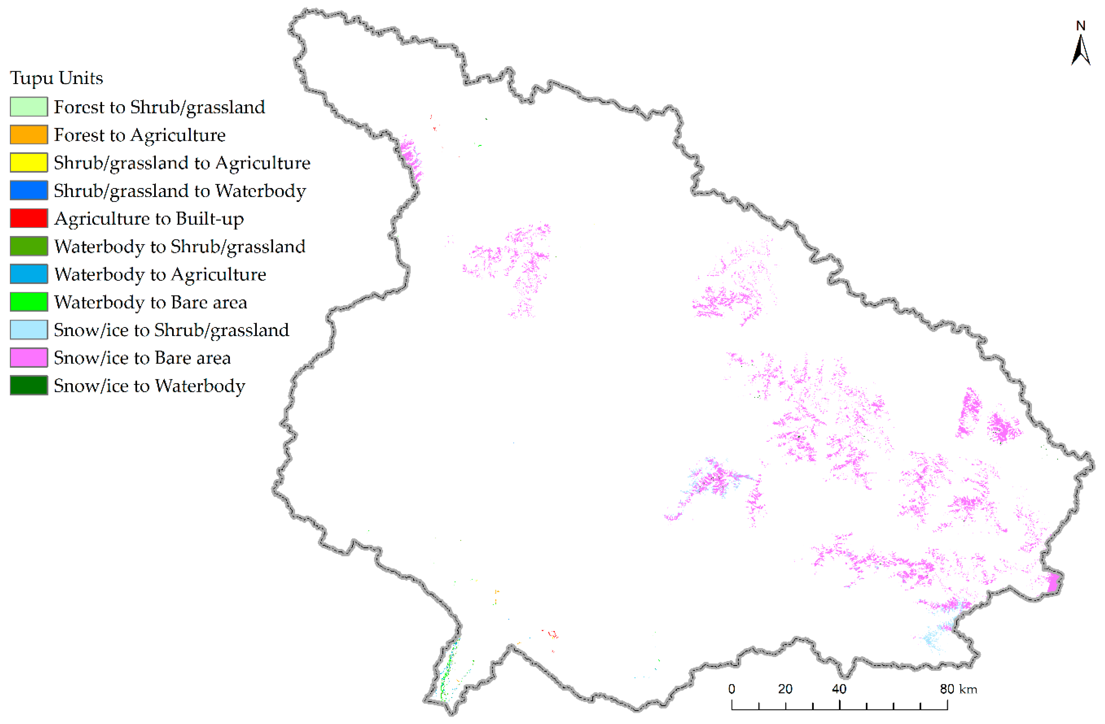
3.5. Analysis by Spatio-Temporal Integrated Methodology—Tupu

The spatial distribution of arisen and shrunken Tupu units in the KRB is shown in Figure 4. Among the arisen Tupu, the largest arising Tupu unit was in the bare area category, followed by shrub/grassland and waterbody areas. The largest shrunken Tupu unit was of snow/ice, followed by waterbody and bare area. The area of arisen and shrunken Tupu units along with their respective ESV for different land cover categories in the KRB is described in Section 3.6.

3.6. Ecosystem Services Value of the Basin

Based on the ESV coefficients derived for the TP in 2003 (Table 2), the total ESV in the basin was $45.87 × 10⁸ in 2000. The ESV value of the forest, shrub/grassland, and agriculture covered the largest ESV value of $33.46 × 10⁸, $6.29 × 10⁸ and $4.23 × 10⁸, respectively, since these three land cover categories occupy 95.9% of the whole basin area.

From the year 2000 to 2010, the ESV had increased by $5 million. The ESV for the categories of forest, shrub/grassland, and agriculture were $33.46 × 10⁸, $6.31 × 10⁸ and $4.27 × 10⁸, respectively, for the year 2010. This increase in total ESV was attributed to the increase in the area of shrub/grassland, agriculture and barren land with forest area almost being stable. During the same period, the ESV of snow/ice decreased from $0.94 × 10⁸ to $0.92 × 10⁸, and that of water bodies decreased from $0.18 × 10⁸ to $0.16 × 10⁸. Conversely, in the period of 2010 to 2017, the total ESV decreased by $3 million in the KRB. From 2010 to 2017, there was a decrease in ESV for the forest, agriculture, water bodies, and snow/ice, whereas, ESV increased for shrub/grassland and barren land (

Table 7. ESV of the KRB. The values in parentheses are after inflation adjustment.

Land Cover Types	ESV (108$)			Change in ESV (106$)
	2000	2010	2017	2000–2017
Forest	33.459	33.458 (39.91)	33.457 (46.545)	−0.1 (13.09)
Shrub/grassland	6.291	6.317(7.535)	6.352 (8.837)	6.12 (2.55)
Agriculture	4.230	4.269 (5.092)	4.231 (5.886)	0.1 (1.66)
Bare Area	0.777	0.798 (0.952)	0.836 (1.163)	5.90 (0.39)
Waterbody	0.935	0.919 (1.096)	0.895 1.245)	−3.90 (0.31)
Snow/Ice	0.183	0.156 (0.186)	0.119 (0.166)	−6.39 (−0.02)
Total	45.87	45.92 (54.77)	45.89 (63.84)	1.59 (17.97)

). Overall, from 2000 to 2017, the ESV in the basin increased by $1.59 × 10⁶. The ESV for the forest, shrub/grassland, and agriculture were $33.46 × 10⁸, $6.35 × 10⁸ and $4.23 × 10⁸, respectively, in 2017. The spatial distribution of ESV is shown in Figure 5. The ESV after adjusting the inflation is higher than the values without inflation adjustment (Table 7). The ESV for the years 2010 and 2017 after inflation adjustment is $54.77 × 10⁸ and $63.84 × 10⁸, respectively, which is higher by $8.85 × 10⁸ and $17.95 × 10⁸ than the respective ESV without inflation adjustment.

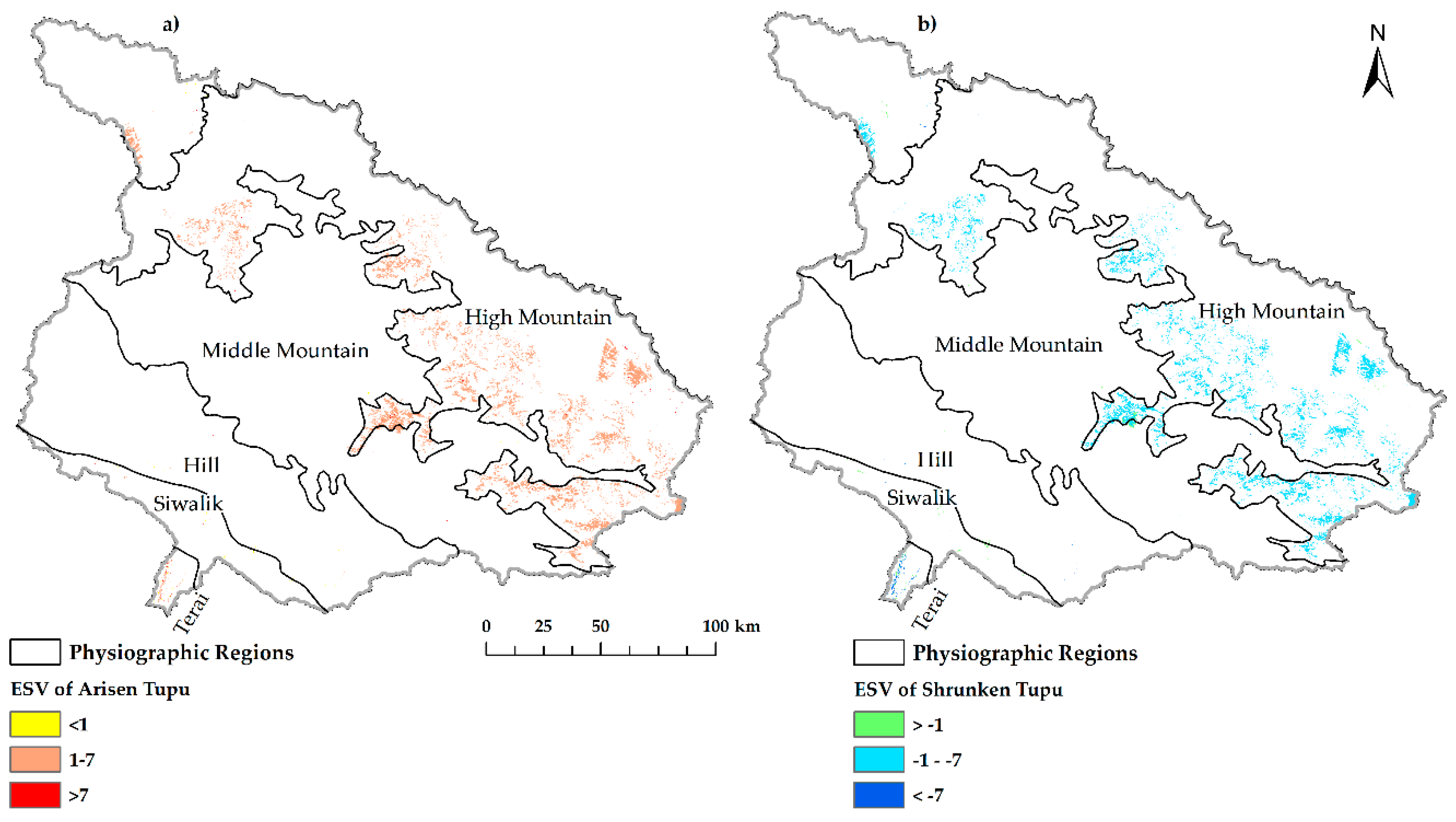
ESV Estimation from Tupu Methodology

ESV gain from the arisen Tupu (arisen ESV) and ESV loss from the shrunken Tupu (shrunken ESV) during 2000–2017 was assessed by multiplying the ESV coefficient with their respective arisen and shrunken land cover categories. For the arisen Tupu, the highest arisen ESV was from increasing waterbody ($8.73 × 10⁶), followed by shrub/grassland ($6.37 × 10⁶) and bare area ($6.02 × 10⁶). For the shrunken Tupu, the highest shrunken ESV was from loss of waterbody ($12.82 × 10⁶) followed by snow/ice ($6.40 × 10⁶) and forest ($0.45 × 10⁶) (

Table 8. Arisen and shrunken Tupu (2000 to 2017) with their respective ESV. The 2017 values in parentheses are after inflation adjustment.

Land Cover Categories	Arisen Tupu		Shrunken Tupu
	Area (×10−2 km2)	Total ESV ($106)	Area (×10−2 km2)	Total ESV ($ 106)
Forest	144	0.31 (0.43)	205.38	−0.45 (−0.62)
Shrub/grassland	8546.58	6.37 (8.86)	312.93	−0.23 (−0.32)
Agriculture	546.66	0.38 (0.53)	412.65	−0.29 (−0.40)
Bare area	100,677.51	6.02 (8.38)	1551.51	−0.09 (−0.13)
Waterbody	1332.18	8.73 (12.14)	1956.06	−12.82 (17.83)
Snow/ice	96.84	0.01 (0.01)	107,216.55	−6.41 (−6.41)
Total		21.82 (30.35)		−20.29 (−28.23)

).

It could be noted that the total gain in ESV ($1.53 × 10⁶) calculated from the addition of arisen ESV and shrunken ESV (Table 8) maintained good agreement with the estimation from the common method (Table 7) as described in Section 3.6, supporting both the methodologies. However, among them, the spatio-temporal integrated Tupu method had a better advantage to show the spatial distribution and characteristics of the ESV across the basin (Figure 5). The major advantage of the spatio-temporal integrated Tupu method is to locate the arisen and shrunken ESV and identify the process of changes it has gone through. This information further allows the users, policymakers, or concerned authority to identify and quantify the changes in the ESV due to LUCC. The shrunken ESV of the forest and agriculture was in the Terai and Siwalik physiographic region of the basin, whereas the shrunken ESV of the snow/ice was in the high mountain region (Figure 5). This shrinkage of snow/ice and conversion to waterbody was a prime factor for the increase in ESV in the high mountain region. The arisen ESV of shrub/grassland is due to the conversion from the bare area in the higher elevation.

4. Discussion

4.1. Mapping of LUCC and Its Dynamics in the KRB

Remote sensing techniques and a geographical information system have been widely used for the LUCC study at local, regional and global scales as they are powerful as well as cost-effective tools to analyze the spatio-temporal variations of the land surface [63,64]. The use of remote sensing techniques has some limitations. The acquisition season and the quality of satellite images (cloud-free) impact the classification scheme [65]. For example, the images from the monsoon period contain high cloud coverage, whereas using images from the winter season can overestimate the temporary snow cover. The significant changes in the categories of shrub/grassland, barren land and snow/ice (Section 3.3) were possibly due to the seasonal variation at the time of satellite image acquisition. In addition, the agricultural area can be misclassified as shrub/grassland when the images used are before the harvesting season. To overcome such limitations, we have used cloud-free and post-monsoon satellite images to maximize classification accuracy.

The KRB has gone through nominal changes in the land cover over a period of seventeen years. The decrease in forest area and increase in the agriculture area was mainly due to anthropogenic activities. The built-up area has increased by 23.14% in the entire basin. The population of Birendranagar municipality of Surkhet district, the largest town in the basin, increased by nearly 70,000 individuals between 2001 and 2015 [59]. Population growth and migration from rural areas to urban areas impact the LUCC [55,59,66]. Thus, the increase in population led to the increase in the built-up area in Surkhet district by 21.64% and in the Burang area by 31.6% from 2000 to 2017. The conversion of 4.06 km² of forest to agriculture, 0.6 km² of forest to built-up and 0.69 km² of forest to shrub/grassland indicate anthropogenic activities responsible for LUCC in the KRB. The study conducted by Uddin et al. [67] on the Kailash Sacred Landscape in the Nepal part (KSL-Nepal), which is also a part of the KRB, suggests that higher dependency on the forest, agricultural expansion, livestock grazing, daily fuelwood consumption, and illegal timber extraction are drivers for the LUCC changes in the region. Birendranagar is the newly declared capital of the Karnali province and, thus, has a high probability of urbanization due to migration. Climate change is also the driving factor for changes in the LUCC. Glacier area has decreased in the KRB by 30% from 1980 to 2010 [68] in the Nepal part and our study also shows a decrease in snow/ice class in the entire transboundary KRB by 35% (Table 5). Snow/ice has largely been converted to bare area (Table 5). The temperature is in increasing trend, while precipitation is in decreasing trend in the basin as mentioned in Section 2.1 [38].

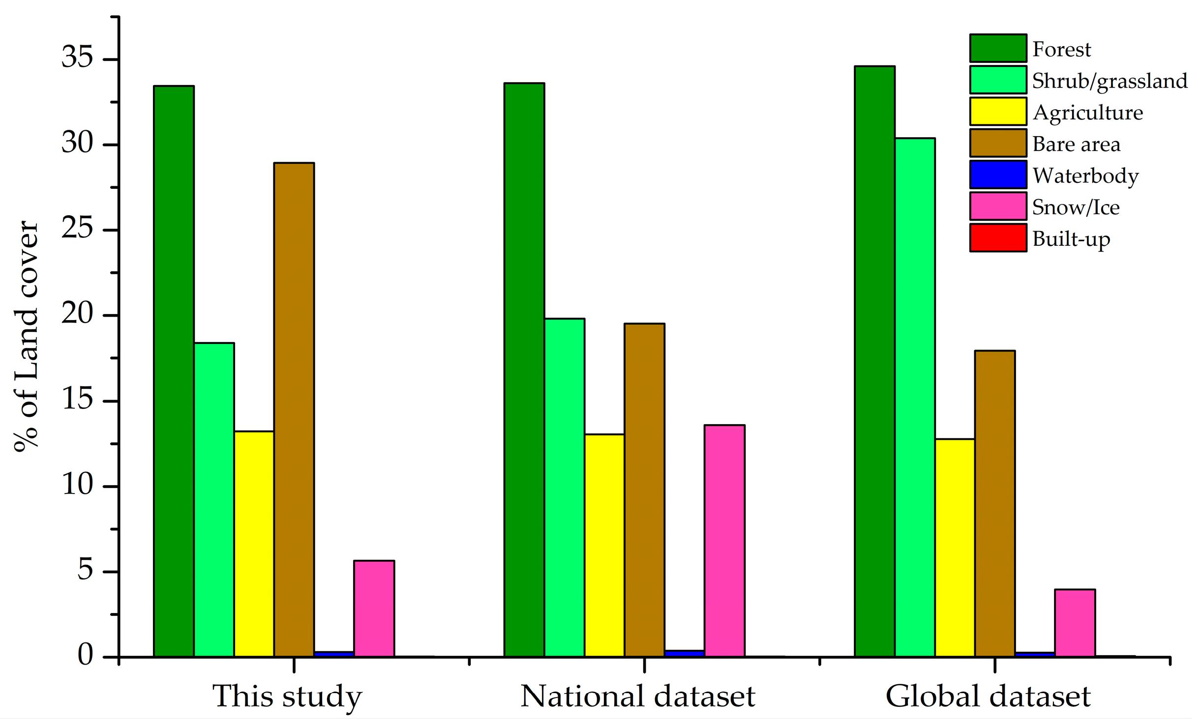
4.2. Global, National, and Regional Dataset Perspectives

Global-level [51] and national-level products [36] in 2010 have dissimilarity in the datasets, especially in the forest land. The area of forest in the KRB reported by Chen et al. [51] while studying global land cover was 15,961.31 km² (34.61%), whereas, Uddin et al. [36] reported the area to be 15,493.84 km² (33.6%) for the year 2010. The two studies differ in the calculation of the total area of grassland and snow/ice (Figure 6). The reason behind the dissimilar data might be due to the methodologies and validation approaches adopted for the classification schemes. The national datasets [36] were more favorable to use over the global datasets [51] because the national datasets were closer to the ground reality [34]. Also, the area of forest (15,426.45 km²) classified in this study is in good agreement with national datasets. The national-level LC of Nepal was validated with field points (435 location points in Google Earth and 130 GPS-tagged field validation points for the accuracy assessment) to rectify the errors [36].

The regional-level land cover data produced for the KRB of the year 2010 in our study was similar to that of national datasets [36] prepared by ICIMOD for the year 2010. The major changes between these two datasets are in the categories of bare area and snow/ice. In the national dataset, bare area has been under classified and the snow/ice has been overclassified. The reason behind these dissimilarities is the image acquisition period. The national dataset acquired data in the winter season, but regional-level data were acquired during the post-monsoon period.

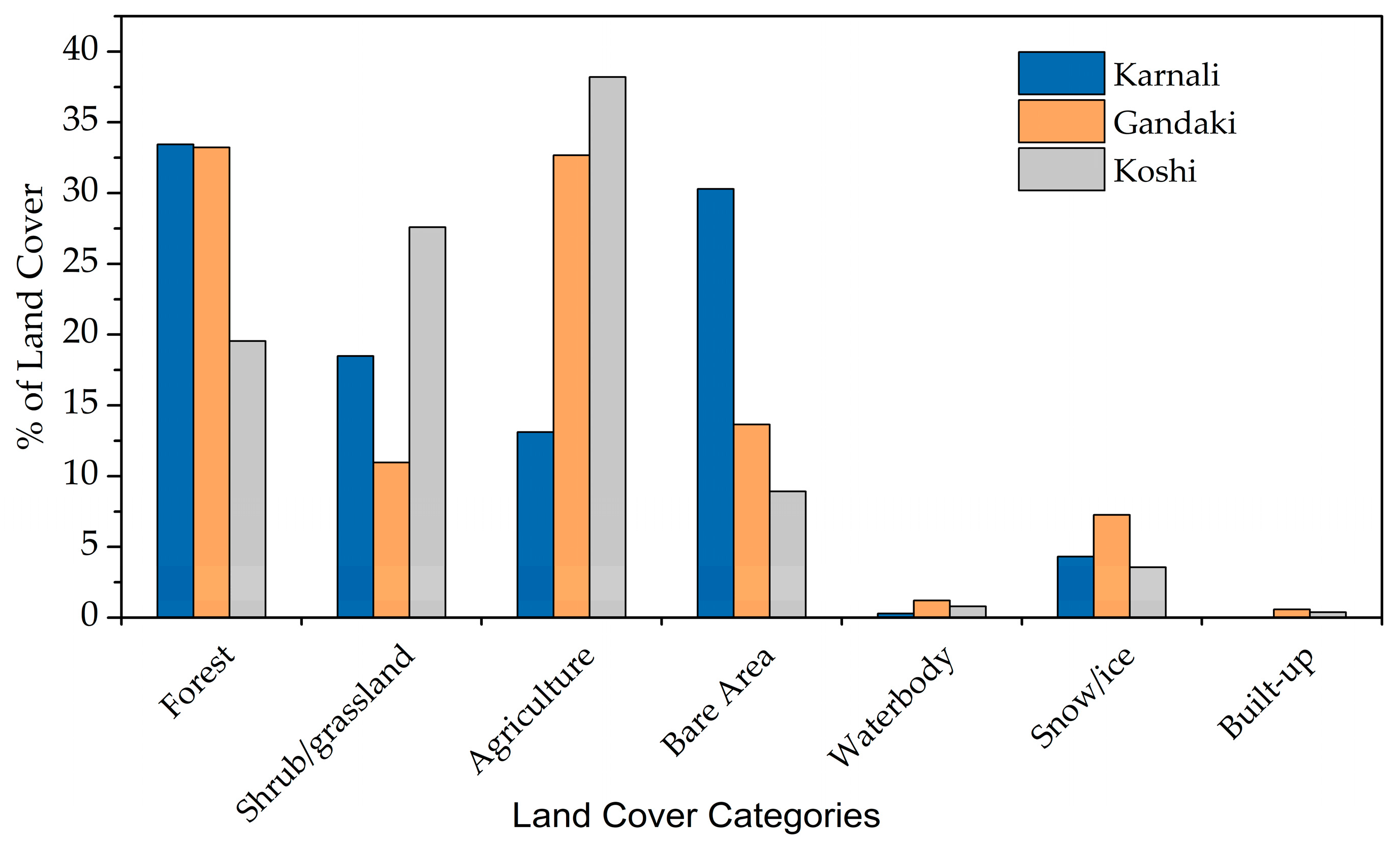
4.3. Comparison of LUCC Dynamics with the Other Two Major Basins in Nepal

Among the three basins, the KRB had the highest coverage of forest (33.45%) and bare area (30.3%). Similarly, the Gandaki basin had the highest coverage of waterbody (1.22%), snow/ice (7.27%) and built-up (0.59%) area, whereas the Koshi basin had the highest coverage of shrub/grassland (27.59%) and agriculture (38.19%) (Figure 7). Comparing LUCC among the three major river basins, it was more rigorous in the Koshi basin followed by the Gandaki basin, with lowest changes in the KRB. In the Koshi basin, cropland, swamp, built-up, shrubland, and grassland have increased, while forest, waterbodies, barren area and snow/ice have decreased between 1990 and 2010. The major changes in the Koshi basin were in the form of forest converted to cropland (4121.78 km²) and barren area converted to grassland (5414.09 km²) [28]. In the Gandaki basin, snow/ice and shrub/grassland area have decreased. However, all other categories have increased from 1990–2015. The forest cover has been increasing in the downstream of the Gandaki basin due to the conservation of the forest by implementing policies and government intervention in the form of various national parks and wildlife reserves [29]. In the KRB, waterbody and snow/ice have decreased and shrub/grassland, agriculture, bare area and built-up have increased during 2000–2017.

Rapid economic and development activities are major factors for LUCC [69,70,71,72]. Urban area expansion of the Kathmandu region and agricultural expansion were the major reasons for LUCC in the Koshi basin [28]. Population growth, migration from rural to urban areas, intensive agricultural practices and land reclamation in the Koshi basin were the prime driving factors for LUCC [29,73,74]. Similarly, urbanization is in increasing trend in Gandaki basin and Rai et al. [29] estimate that the built-up area had increased up by threefold from 1990 to 2015 in the basin. However, urbanization in the KRB was less than in the other two basins. The economic activities are very limited in the KRB. It is one of the most under-developed regions in Nepal facing various conservation and development challenges [67,75] and had the least human development index of 0.386 [76]. Thus, LUCC in the KRB basin was less than the other two basins in Nepal. The accessibility in the Terai region is easier and has experienced more economic and development activities than in hills and mountain area of the KRB [59]. Thus, the KRB region requires proper maintenance of the land cover database for future references as well as proper planning for resource utilization.

4.4. Status of ESV

The ESV in KRB has increased by $1.59 × 10⁶ from 2000 to 2017. This change in ESV is also in accordance with the positive change in ESV in the Gandaki River Basin which is adjacent to the KRB. The gain in ESV in the KRB was largely due to the arisen ESV of shrub/grassland, bare area, and waterbody (in the higher elevation) in the basin. This increase in the ESV of shrub/grassland further implies better ecosystem services. The shrub/grassland ecosystem are key habitats for different animals and particularly serve as pasture for cattle [77]. The ESV coefficient for the bare area and snow/ice category is the same, i.e., $59.83 per hectare [27] and, thus, the change from snow/ice to the bare area or vice-versa does not affect the ESV. In the high altitude region, the conversion of snow/ice to waterbody (Table 5) increased the total ESV, as the coefficient for waterbody is more than 100 times higher than that of snow/ice (Table 2). This result might show the improvement of ESV. However, in the high altitude region, the increase in the area of waterbody is primarily due to glacial lake expansion [39], which increases the risk of glacier lake outburst flood (GLOF), threatening the downstream communities and infrastructures [78]. Thus, the increase in ESV (from the conversion of snow/ice to waterbody) does not necessarily indicates benefit in the mountain ecosystem. The waterbodies in the lower elevation need to be preserved as the shrunken ESV from waterbody is the highest. The shrunken ESV of forest, agriculture, and waterbody in the lower elevation have contributed to a decrease in ESV. The diminishing ESV due to shrunken forest and agriculture in the lower elevation indicate the human activities responsible for deteriorating the ESV in the basin.

The inflation adjusted ESV is higher than the ESV without inflation adjustment. Even the same area of any LC category in two different time period would show an increase in ESV with inflation adjustment. Here, in our study, the forest area has decreased from the year 2000 to 2017. However, with inflation adjustment, the ESV of forest has increased from $33.46 × 108 in 2000 to $46.55 × 108 in 2017, implying betterment in forest ecosystem. But the decrease in forest area actually implies degradation in the forest ecosystem [79,80]. For a temporal comparison of changes in the ESV, the values without inflation adjustment give a better understanding of the changes in the ESV. We recommend that new ESV coefficients need to be derived to represent the actual ESV in a given time, rather than use the adjusted inflation to compare the ESV for the different time period.

From 1997 to 2011, the loss in global ecosystem services due to LUCC was about $4.3–20.2 trillion [22]. In the Tibetan Plateau, the ESV increased at the rate of $67.10 × 10⁸ from the year 1985 to 2000 [81]. However, from 2000 to 2010, the ESV in the TP decreased at the rate of $9.30 × 10⁸ [82]. Climate warming and socio-economic development degrading the environmental–ecological system [32] coupled with rampant urbanization [83] are the major factors for the decrease in ESV in the TP. The ecosystem services value (ESVs) for the Koshi river basin for the years 1990 and 2010 were $91.60 × 10⁸ and $89.55 × 10⁸, respectively, with a decrease of $2.05 × 10⁸ [28] over the period. In the Gandaki river basin, the ESV for the years 1990 and 2015 were $50.6 × 10⁸ and $51.84 × 10⁸, respectively, with an increase of $1.68 × 10⁸ [29]. In the Koshi basin, the loss is primarily due to anthropogenic activities such as urbanization, deforestation and land reclamation [28]. Whereas in the Gandaki basin, ecosystem services have improved due to the increase in cropland, forest, river/lake, wetland categories. The LUCC and ESV change in the KRB was less than that of Gandaki River Basin and Koshi River Basin. The ecosystem services have improved in the KRB and Gandaki basin [29], whereas they have deteriorated in Koshi River Basin [28]. Significant LUCC in the Gandaki and Koshi River basin amounted to significant changes in the ESV. Also, the temporal span of the data used for the Koshi basin (20 years) and Gandaki basin (25 years) were longer than that of the KRB (17 years). With new federal state government coming into the act, major development programs in the KRB are in the pipeline [84]. Thus, LUCC due to development activities will inevitably be affected, influencing the ESV of the basin in the future. Sustainable landscape planning, management, and development measures have to be adopted in this region [67,85] and the region is still facing challenges with the effectiveness of protected area management [86]. The mapping of arisen ESV and shrunken ESV thus can put forward the spatial location that needs immediate attention, aiding in the management of ecosystem services.

5. Conclusions

In this study, we have investigated the variation in land use and land cover in the transboundary KRB using optical satellite data for a period of seventeen years from 2000 to 2017. Furthermore, we have evaluated and analyzed the ESV for each land cover type. Forest covered the highest area in the basin, followed by bare area, shrub/grassland, agriculture, snow/ice, waterbody and built-up for the year 2017. Forest, waterbody, and snow/ice have decreased, whereas shrub/grassland, agriculture, bare area and built-up have increased in the basin in the study period. Due to these LUCC, the total ESV for the basin increased by $1.59 × 10⁶ in the last 17 years, and this gain occurred mainly in shrub/grassland, agriculture, bare area, and water bodies (in the higher altitude) ecosystem. The highest decrease was in the snow/ice ecosystem, followed by waterbody and forest ecosystem, respectively. The LUCC and its effects in the ESV are further spatially shown in the form of arisen and shrunken Tupu units. The arisen ESV was highest for waterbody ($8.73 × 10⁶) in the higher altitude, followed by shrub/grassland ($6.37 × 10⁶) and bare area ($6.02 × 10⁶). The shrunken ESV was highest for waterbody ($12.82 × 10⁶) followed by snow/ice ($6.41 × 10⁶) and forest ($0.45 × 10⁶). The small increase in the ESV shows the improving ecosystem services and LUCC is one of the driving factors for the changes in ESV in the basin. Thus, regular monitoring of the dynamics of LUCC is essential. The spatio-temporal integrated geo-information landscape Tupu methodology had a major advantage over the common method as it shows the spatial distribution and change characteristics of the LUCC as well as arisen and shrunken ESV across the basin, which is an important contribution to the LULC, LUCC, and ESV related studies. The spatial distribution of LUCC and changes in ESV extracted by using spatio-temporal integrated landscape information Tupu methodology facilitates in better understanding the spatio-temporal dynamics of LUCC and changes in ESV.

The usage of high-resolution satellite images can give a better classification results improving the estimation of ESV, which can assist in natural resource sustainable management and adaptations of ecosystem services at the regional and local scale.

References

1. Lambin, E.F.; Turner, B.L.; Geist, H.J.; Agbola, S.B.; Angelsen, A.; Bruce, J.W.; Coomes, O.T.; Dirzo, R.; Fischer, G.; Folke, C.; et al. The causes of land-use and land-cover change: Moving beyond the myths. Glob. Environ. Chang. 2001, 11, 261–269. [Google Scholar] [CrossRef]
2. Jordan, M.; Meyer, W.B.; Kates, R.W.; Clark, W.C.; Richards, J.F.; Turner, B.L.; Mathews, J.T. The Earth as Transformed by Human Action: Global and Regional Changes in the Biosphere over the Past 300 Years; CUP Archive: Cambridge, UK, 1990. [Google Scholar]
3. Vitousek, P.M. Beyond global warming—Ecology and global change. Ecology 1994, 75, 1861–1876. [Google Scholar] [CrossRef]
4. Lambin, E.; Baulies, X.; Bockstael, N.; Fischer, G.; Krug, T.; Leemans, R.; Moran, E.; Rindfuss, R.; Sato, Y.; Skole, D. Land Use and Cover Change Implementation Strategy; IGBP Report No. 48; IGBP: Stockholm, Sweden, 1999. [Google Scholar]
5. Di Gregorio, A. Land Cover Classification System: Classification Concepts and User Manual: Lccs; Food & Agriculture Org.: Rome, Italy, 2005; Volume 8. [Google Scholar]
6. Kindu, M.; Schneider, T.; Teketay, D.; Knoke, T. Changes of ecosystem service values in response to land use/land cover dynamics in Munessa–Shashemene landscape of the Ethiopian highlands. Sci. Total Environ. 2016, 547, 137–147. [Google Scholar] [CrossRef]
7. Xu, C.Y.; Pu, L.J.; Zhu, M.; Li, J.G.; Chen, X.J.; Wang, X.H.; Xie, X.F. Ecological security and ecosystem services in response to land use change in the coastal area of Jiangsu, China. Sustainability 2016, 8, 816. [Google Scholar] [CrossRef]
8. Sala, O.E.; Chapin, F.S., III; Armesto, J.J.; Berlow, E.; Bloomfield, J.; Dirzo, R.; Huber-Sanwald, E.; Huenneke, L.F.; Jackson, R.B.; Kinzig, A.; et al. Global biodiversity scenarios for the year 2100. Science 2000, 287, 1770–1774. [Google Scholar] [CrossRef] [PubMed]
9. Chapin, F.S., III; Matson, P.A.; Vitousek, P. Principles of Terrestrial Ecosystem Ecology; Springer Science & Business Media: Berlin, Germany, 2011. [Google Scholar]
10. Chase, T.N.; Pielke, R.A.; Kittel, T.G.F.; Nemani, R.R.; Running, S.W. Simulated impacts of historical land cover changes on global climate in Northern Winter. Clim. Dyn. 2000, 16, 93–105. [Google Scholar] [CrossRef]
11. Houghton, R.A.; Hackler, J.L.; Lawrence, K.T. The US carbon budget: Contributions from land-use change. Science 1999, 285, 574–578. [Google Scholar] [CrossRef]
12. Yan, M.; Liu, J.; Wang, Z.Y. Global climate responses to land use and land cover changes over the past two millennia. Atmosphere 2017, 8, 64. [Google Scholar] [CrossRef]
13. Vitousek, P.M.; Mooney, H.A.; Lubchenco, J.; Melillo, J.M. Human domination of Earth’s ecosystems. Science 1997, 277, 494–499. [Google Scholar] [CrossRef]
14. Kasperson, J.X.; Kasperson, R.E.; Turner, B.L. Regions at Risk; United Nations University Press: Tokyo, Japan, 1995. [Google Scholar]
15. Sharma, E.; Chettri, N.; Tse-Ring, K.; Shrestha, A.; Jing, F.; Mool, P.; Eriksson, M. Climate Change Impacts and Vulnerability in the Eastern Himalayas; ICIMOD: Patan, Nepal, 2009. [Google Scholar]
16. Bajracharya, B.; Uddin, K.; Chettri, N.; Shrestha, B.; Siddiqui, S.A. Understanding land cover change using a harmonized classification system in the Himalaya a case study from Sagarmatha National Park, Nepal. Mt. Res. Dev. 2010, 30, 143–156. [Google Scholar] [CrossRef]
17. Costanza, R.; d’Arge, R.; de Groot, R.; Farber, S.; Grasso, M.; Hannon, B.; Limburg, K.; Naeem, S.; O’Neill, R.V.; Paruelo, J.; et al. The value of the world’s ecosystem services and natural capital. Nature 1997, 387, 253–260. [Google Scholar] [CrossRef]
18. World Resources Institute. Ecosystem and Human Well-Being: Biodiversity Synthesis; World Resources Institute: Washington, DC, USA, 2005. [Google Scholar]
19. Daily, G.C. Nature’s Services; Island Press: Washington, DC, USA, 1997. [Google Scholar]
20. Yongmin, Z.; Shidong, Z.; Rongchao, G. Recent advances and challenges in ecosystem service research. J. Resour. Ecol. 2014, 5, 82–90. [Google Scholar] [CrossRef]
21. De Groot, R.; Brander, L.; Van Der Ploeg, S.; Costanza, R.; Bernard, F.; Braat, L.; Christie, M.; Crossman, N.; Ghermandi, A.; Hein, L. Global estimates of the value of ecosystems and their services in monetary units. Ecosyst. Serv. 2012, 1, 50–61. [Google Scholar] [CrossRef]
22. Costanza, R.; de Groot, R.; Sutton, P.; van der Ploeg, S.; Anderson, S.J.; Kubiszewski, I.; Farber, S.; Turner, R.K. Changes in the global value of ecosystem services. Glob. Environ. Chang. 2014, 26, 152–158. [Google Scholar] [CrossRef]
23. Song, W.; Deng, X. Land-use/land-cover change and ecosystem service provision in China. Sci. Total Environ. 2017, 576, 705–719. [Google Scholar] [CrossRef] [PubMed]
24. Xie, H.L.; Yao, G.R.; Liu, G.Y. Spatial evaluation of the ecological importance based on Gis for environmental management: A case study in Xingguo County of China. Ecol. Indic. 2015, 51, 3–12. [Google Scholar] [CrossRef]
25. Gong, J.; Li, J.Y.; Yang, J.X.; Li, S.C.; Tang, W.W. Land use and land cover change in the Qinghai Lake Region of the Tibetan Plateau and its impact on ecosystem services. Int. J. Environ. Res. Public Health 2017, 14, 818. [Google Scholar] [CrossRef]
26. Dendoncker, N.; Keune, H.; Jacobs, S.; Gómez-Baggethun, E. Inclusive ecosystem services valuation. In Ecosystem Services; Jacobs, S., Dendoncker, N., Keune, H., Eds.; Elsevier: Amsterdam, The Netherlands, 2014; pp. 3–12. [Google Scholar]
27. Xie, G.-D.; Lu, C.-X.; Leng, Y.-F.; Zheng, D.; Li, S. Ecological assets valuation of the Tibetan Plateau. J. Nat. Resour. 2003, 18, 189–196. [Google Scholar]
28. Zhilong, Z.; Xue, W.; Yili, Z.; Jungang, G. Assessment of changes in the value of ecosystem services in the Koshi River Basin, Central High Himalayas based on land cover changes and the Ca-Markov model. J. Resour. Ecol. 2017, 8, 67–76. [Google Scholar] [CrossRef]
29. Rai, R.; Zhang, Y.L.; Paudel, B.; Acharya, B.K.; Basnet, L. Land use and land cover dynamics and assessing the ecosystem service values in the trans-boundary Gandaki River Basin, Central Himalayas. Sustainability 2018, 10, 3052. [Google Scholar] [CrossRef]
30. Immerzeel, W.; Stoorvogel, J.; Antle, J. Can payments for ecosystem services secure the water tower of Tibet? Agric. Syst. 2008, 96, 52–63. [Google Scholar] [CrossRef]
31. Qiang, W.; Xi, C.; Degang, Y.; Changjian, W. Paying for Tibet’s environmental-ecosystem services. Environ. Sci. Technol. 2012, 46, 5264. [Google Scholar] [CrossRef] [PubMed]
32. Yu, C.; Zhang, Y.; Zeng, R.; Zhang, X.; Wang, J. Ecological and Environmental Issues Faced by a Developing Tibet; ACS Publications: Washington, DC, USA, 2012. [Google Scholar]
33. Zhu, J.; Zhou, Y.; Wang, S.; Wang, L.; Wang, F.; Liu, W.; Guo, B. Multicriteria decision analysis for monitoring ecosystem service function of the three-river headwaters region of the Qinghai-Tibet Plateau, China. Environ. Monit. Assess. 2015, 187, 355. [Google Scholar] [CrossRef] [PubMed]
34. Paudel, B.; Zhang, Y.L.; Li, S.C.; Liu, L.S.; Wu, X.; Khanal, N.R. Review of studies on land use and land cover change in Nepal. J. Mt. Sci. 2016, 13, 643–660. [Google Scholar] [CrossRef]
35. Ye, Q.; Tian, G.; Li, X.; Chen, S. Tupu methods of spatio-temporal analysis on land use/land cover change—A case study in the Yellow River Delta. In Proceedings of the IEEE 2004 Geoscience and Remote Sensing Symposium (IGARSS’04), Anchorage, AK, USA, 20–24 September 2004; pp. 749–752. [Google Scholar]
36. Uddin, K.; Shrestha, H.L.; Murthy, M.S.; Bajracharya, B.; Shrestha, B.; Gilani, H.; Pradhan, S.; Dangol, B. Development of 2010 national land cover database for the Nepal. J. Environ. Manag. 2015, 148, 82–90. [Google Scholar] [CrossRef] [PubMed]
37. Yao, T.; Thompson, L.; Yang, W.; Yu, W.; Gao, Y.; Guo, X.; Yang, X.; Duan, K.; Zhao, H.; Xu, B. Different glacier status with atmospheric circulations in Tibetan Plateau and surroundings. Nat. Clim. Chang. 2012, 2, 663. [Google Scholar] [CrossRef]
38. Khatiwada, K.R.; Panthi, J.; Shrestha, M.L.; Nepal, S. Hydro-climatic variability in the Karnali River Basin of Nepal Himalaya. Climate 2016, 4, 17. [Google Scholar] [CrossRef]
39. Khadka, N.; Zhang, G.; Thakuri, S. Glacial lakes in the Nepal Himalaya: Inventory and decadal dynamics (1977–2017). Remote Sens. 2018, 10, 1913. [Google Scholar] [CrossRef]
40. Farr, T.G.; Rosen, P.A.; Caro, E.; Crippen, R.; Duren, R.; Hensley, S.; Kobrick, M.; Paller, M.; Rodriguez, E.; Roth, L.; et al. The shuttle radar topography mission. Rev. Geophys. 2007, 45, 2. [Google Scholar] [CrossRef]
41. Civco, D.L.; Hurd, J.D.; Wilson, E.H.; Song, M.; Zhang, Z. A Comparison of Land Use and Land Cover Change Detection Methods. In Proceedings of the ASPRS-ACSM Annual Conference, Washington, DC, USA, 19–26 April 2002. [Google Scholar]
42. Yoon, G.; Cho, S.; Chae, G.; Park, J. Automatic land-cover classification of landsat images using feature database in a network. In Proceedings of the IGARSS 2005 symposium, Seoul, Korea, 25–29 July 2005. [Google Scholar]
43. Harken, J.; Sugumaran, R. Classification of Iowa Wetlands using an airborne hyperspectral image: A comparison of the spectral angle mapper classifier and an object-oriented approach. Can. J. Remote Sens. 2005, 31, 167–174. [Google Scholar] [CrossRef]
44. Gao, Y.; Mas, J.; Niemeyer, I.; Marpu, P.; Palacio, J. Object based image analysis for forest area land cover mapping. In Proceedings of the International Symposium for Spatial Data Quality (ISSDQ), Enschede, The Netherlands, 13–15 June 2007; pp. 13–15. [Google Scholar]
45. Blaschke, T.; Lang, S.; Lorup, E.; Strobl, J.; Zeil, P. Object-oriented image processing in an integrated gis/remote sensing Environment and perspectives for environmental applications. Environ. Inf. Plan. Politics Public 2000, 2, 555–570. [Google Scholar]
46. Benz, U.C.; Hofmann, P.; Willhauck, G.; Lingenfelder, I.; Heynen, M. Multi-resolution, object-oriented fuzzy analysis of remote sensing data for gis-ready information. ISPRS J. Photogramm. 2004, 58, 239–258. [Google Scholar] [CrossRef]
47. Blaschke, T. Object based image analysis for remote sensing. ISPRS J. Photogramm. 2010, 65, 2–16. [Google Scholar] [CrossRef] [Green Version]
48. Hay, G.J.; Blaschke, T.; Marceau, D.J.; Bouchard, A. A comparison of three image-object methods for the multiscale analysis of landscape structure. ISPRS J. Photogramm. 2003, 57, 327–345. [Google Scholar] [CrossRef]
49. Hay, G.J.; Castilla, G. Geographic object-based image analysis (Geobia): A new name for a new discipline. In Object-Based Image Analysis; Springer: Berlin, Germany, 2008; pp. 75–89. [Google Scholar]
50. Uddin, K.; Matin, M.A.; Maharjan, S. Assessment of land cover change and its impact on changes in soil erosion risk in Nepal. Sustainability 2018, 10, 4715. [Google Scholar] [CrossRef]
51. Chen, J.; Chen, J.; Liao, A.; Cao, X.; Chen, L.; Chen, X.; He, C.; Han, G.; Peng, S.; Lu, M. Global land cover mapping at 30 m resolution: A pok-based operational approach. ISPRS J. Photogramm. 2015, 103, 7–27. [Google Scholar] [CrossRef]
52. Congalton, R.G. A review of assessing the accuracy of classifications of remotely sensed data. Remote Sens. Environ. 1991, 37, 35–46. [Google Scholar] [CrossRef]
53. Rwanga, S.S.; Ndambuki, J. Accuracy assessment of land use/land cover classification using remote Sensing and gis. Int. J. Geosci. 2017, 8, 611. [Google Scholar] [CrossRef]
54. Tilahun, A.; Teferie, B. Accuracy assessment of land use land cover classification using Google Earth. Am. J. Environ. Prot. 2015, 4, 193–198. [Google Scholar] [CrossRef]
55. Xue, W.; Jungang, G.; Yili, Z.; Linshan, L.; Zhilong, Z.; Paudel, B. Land cover status in the Koshi River Basin, Central Himalayas. J. Resour. Ecol. 2017, 8, 10–19. [Google Scholar] [CrossRef]
56. Hu, Q.; Wu, W.; Xia, T.; Yu, Q.; Yang, P.; Li, Z.; & Song, Q. Exploring the use of Google Earth imagery and object-based methods in land use/cover mapping. Remote Sens. 2013, 5, 6026–6042. [Google Scholar] [CrossRef]
57. Paudyal, K.; Baral, H.; Putzel, L.; Bhandari, S.; Keenan, R. Change in land use and ecosystem services delivery from community-based forest landscape restoration in the Phewa Lake Watershed, Nepal. Int. For. Rev. 2017, 19, 88–101. [Google Scholar] [CrossRef]
58. Regmi, R.; Saha, S.; Balla, M. Geospatial analysis of land use land cover change modeling at Phewa Lake Watershed of Nepal by using cellular automata Markov model. Int. J. Curr. Eng. Technol. 2014, 4, 2617–2627. [Google Scholar]
59. Rijal, S.; Rimal, B.; Sloan, S. Flood hazard mapping of a rapidly urbanizing city in the Foothills (Birendranagar, Surkhet) of Nepal. Land 2018, 7, 60. [Google Scholar] [CrossRef]
60. Su, W.; Liang, D.; Tang, G.; Xiao, Z.; Li, J.; Wan, Z.; Li, P. Landsat-based long–term lucc mapping in Xinlicheng Reservoir Basin using object-based classification. In IOP Conference Series: Earth and Environmental Science; IOP Publishing: Bristol, UK, 2017; Volume 64, p. 012024. [Google Scholar] [CrossRef]
61. Paudel, B.; Gao, J.G.; Zhang, Y.L.; Wu, X.; Li, S.C.; Yan, J.Z. Changes in cropland status and their driving factors in the Koshi River Basin of the Central Himalayas, Nepal. Sustainability 2016, 8, 933. [Google Scholar] [CrossRef]
62. Ye, Q.H.; Liu, G.H.; Tian, G.L.; Chen, S.L.; Huang, C.; Chen, S.P.; Liu, Q.S.; Chang, J.; Shi, Y. Geospatial-temporal analysis of land-use changes in the Yellow River delta during the Last 40 Years. Sci. China Ser. D 2004, 47, 1008–1024. [Google Scholar] [CrossRef]
63. Hu, H.-B.; Liu, H.-Y.; Hao, J.-F.; An, J. Analysis of land use change characteristics based on remote sensing and gis in the Jiuxiang River Watershed. Int. J. Smart Sens. Intell. Syst. 2012, 5. [Google Scholar] [CrossRef]
64. Lucas, I.; Janssen, F.; van der Wel, F.J. Accuracy assessment ofsatellite derived landcover data: A review. Photogramm. Eng. Remote Sens. 1994, 60, 426–479. [Google Scholar]
65. Gilani, H.; Shrestha, H.L.; Murthy, M.S.; Phuntso, P.; Pradhan, S.; Bajracharya, B.; Shrestha, B. Decadal land cover change dynamics in Bhutan. J. Enviorn. Manag. 2015, 148, 91–100. [Google Scholar] [CrossRef]
66. Song, X.; Yang, G.X.; Yan, C.Z.; Duan, H.C.; Liu, G.Y.; Zhu, Y.L. Driving forces behind land use and cover change in the Qinghai-Tibetan Plateau: A case study of the source region of the Yellow River, Qinghai Province, China. Environ. Earth Sci. 2009, 59, 793–801. [Google Scholar] [CrossRef]
67. Uddin, K.; Chaudhary, S.; Chettri, N.; Kotru, R.; Murthy, M.; Chaudhary, R.P.; Ning, W.; Shrestha, S.M.; Gautam, S.K. The changing land cover and fragmenting forest on the roof of the world: A case study in Nepal’s Kailash sacred landscape. Landsc. Urban Plan. 2015, 141, 1–10. [Google Scholar] [CrossRef]
68. Bajracharya, S.R.; Maharjan, S.B.; Shrestha, F.; Bajracharya, O.R.; Baidya, S. Glacier Status in Nepal and Decadal Change from 1980 to 2010 Based on Landsat Data; International Centre for Integrated Mountain Development: Patan, Nepal, 2014. [Google Scholar]
69. Tsarouchi, G.M.; Mijic, A.; Moulds, S.; Buytaert, W. Historical and future land-cover changes in the upper Ganges Basin of India. Int. J. Remote Sens. 2014, 35, 3150–3176. [Google Scholar] [CrossRef]
70. Wang, X.; Zheng, D.; Shen, Y. Land use change and its driving forces on the Tibetan Plateau during 1990–2000. Catena 2008, 72, 56–66. [Google Scholar] [CrossRef]
71. Liu, J.Y.; Kuang, W.H.; Zhang, Z.X.; Xu, X.L.; Qin, Y.W.; Ning, J.; Zhou, W.C.; Zhang, S.W.; Li, R.D.; Yan, C.Z.; et al. Spatiotemporal characteristics, patterns, and causes of land-use changes in China since the late 1980s. J. Geogr. Sci. 2014, 24, 195–210. [Google Scholar] [CrossRef]
72. Cui, X.F.; Graf, H.F. Recent land cover changes on the Tibetan Plateau: A Review. Clim. Chang. 2009, 94, 47–61. [Google Scholar] [CrossRef]
73. Rimal, B. Urbanization and the decline of agricultural land in Pokhara sub-metropolitan city, Nepal. J. Agric. Sci. 2012, 5, 54. [Google Scholar] [CrossRef]
74. Massey, D.S.; Axinn, W.G.; Ghimire, D.J. Environmental change and out-migration: Evidence from Nepal. Popul. Environ. 2010, 32, 109–136. [Google Scholar] [CrossRef] [PubMed]
75. Roy, R.; Schmidt-Vogt, D.; Myrholt, O. “Humla Development Initiatives” for better livelihoods in the face of isolation and conflict. Mt. Res. Dev. 2009, 29, 211–219. [Google Scholar] [CrossRef]
76. GoN. Nepal Human Development Report 2014; Nepal Planning Commission: Kathmandu, Nepal, 2014. [Google Scholar]
77. Richard, C.; Basnet, K.; Sah, J.P.; Raut, Y. Grassland Ecology and Management in Protected Areas of Nepal; ICIMOD: Patan, Nepal, 2000; Volume 12000. [Google Scholar]
78. Rounce, D.R.; Watson, C.S.; McKinney, D.C. Identification of hazard and risk for glacial lakes in the Nepal Himalaya using satellite imagery from 2000–2015. Remote Sens. 2017, 9, 654. [Google Scholar] [CrossRef]
79. Chaudhary, R.P.; Uprety, Y.; Rimal, S.K. Deforestation in Nepal: Causes, consequences, and responses. In Biological and Environmental Hazards, Risks, and Disasters; Sivanpillai, R., Shroder, J.F., Eds.; Elsevier: Amsterdam, The Nethetrlands, 2016; pp. 335–372. [Google Scholar]
80. Bajracharya, D. Deforestation in the food/fuel context: Historical and political perspectives from Nepal. Mt. Res. Dev. 1983, 3, 227–240. [Google Scholar] [CrossRef]
81. Liu, J.; Gao, J.; Nie, Y. Measurement and dynamic changes of ecosystem services value for the Tibetan Plateau based on remote sensing techniques. Geogr. Geoinf. Sci. 2009, 3, 17–29. [Google Scholar]
82. Liu, X.; Ren, Z.; Lin, Z. Dynamic assessment of the values of Co2 fixation and O2 release in Qinghai-Tibet Plateau ecosystem. Geogr. Res. 2013, 32, 663–670. [Google Scholar]
83. Mou, X.; Zhao, X.; Rao, S. Changes of ecosystem structure in Qinghai-Tibet Plateau ecological barrier area during recent ten years. Acta Sci. Nat. Univ. Pekin. 2016, 52, 279–286. [Google Scholar]
84. N.P. Commission. Nepal and the Millennium Development Goals Final Status Report 2000–2015; N.P. Commission: Kathmandu, Nepal, 2016. [Google Scholar]
85. Schild, A. Icimod’s position on climate change and mountain systems: The case of the Hindu Kush–Himalayas. Mt. Res. Dev. 2008, 28, 328–331. [Google Scholar] [CrossRef]
86. Oli, K.P.; Chaudhary, S.; Sharma, U.R. Are governance and management effective within protected areas of the Kanchenjunga landscape (Bhutan, India and Nepal). Parks 2013, 19, 25–36. [Google Scholar] [CrossRef]
Figure 1. Location of the study area, i.e., the Karnali river basin.
Sustainability 11 03183 g001
Figure 2. The framework of the study.
Sustainability 11 03183 g002
Figure 3. Land cover maps of the KRB for (a) 2000; (b) 2010 and (c) 2017.
Sustainability 11 03183 g003
Figure 4. Arisen Tupu (a) and shrunken Tupu (b) in the KRB from 2000–2017.
Sustainability 11 03183 g004
Figure 5. Spatial distribution of (a) arisen ESV and (b) shrunken ESV in the KRB (ESV units in 106 $).
Sustainability 11 03183 g005
Figure 6. Comparison of land cover categories (%) of this study with National [36] and Global [51] datasets for 2010 in the KRB.
Sustainability 11 03183 g006
Figure 7. Land cover (%) for different classes in the KRB (2017), Gandaki (2015) [29] and Koshi (2010) [28] basin in Nepal.
Sustainability 11 03183 g007