A Study on the Relationship between Analysts’ Cash Flow Forecasts Issuance and Accounting Information: Evidence from Korea

1
Department of Accounting, College of Social Sciences, Sunchon National University, Jeonnam 57922, Korea
2
School of Business, Hanyang University, Seoul 04763, Korea
*
Author to whom correspondence should be addressed.
Sustainability 2019, 11(12), 3399; https://0-doi-org.brum.beds.ac.uk/10.3390/su11123399
Submission received: 18 May 2019
/
Revised: 15 June 2019
/
Accepted: 17 June 2019
/
Published: 20 June 2019
(This article belongs to the Section Economic and Business Aspects of Sustainability)
Abstract
:This study analyzes the relationship between the future cash flow forecast information provided by financial analysts and accounting information. We examine whether the joint issuance of financial analyst earnings forecasts and cash flow forecasts from 2011 to 2015 contributes to the information usefulness of Korean listed firms. The empirical results of this study are as follows. First, the issuance of analysts’ cash flow forecasts and earnings forecast accuracy were significant positive values. Cash flow forecast accuracy and earnings forecast accuracy were significant positive values. Second, the issuance of analysts’ cash flow forecasts and buy–sell bid spread are significant negative values. These results show that the information asymmetry between the manager and the investor can be reduced based on the rich information environment. This study suggests that cash flow forecasting information of financial analysts provides important evidence for capital market participants because it provides evidence that capital market participants’ information can be used as useful information for economic decision-making. These results show the sustainability of a firm from the viewpoint of a financial analyst who acts as an intermediary and external supervisor in the capital market. In addition, the analysts’ cash flow forecasting information is expected to reduce the information asymmetry between the company and the investor, thereby increasing the transparency and sustainability of the firm.
1. Introduction
The value of a firm is determined by the present value of future cash flows. Future cash flows are predicted using various information because it is difficult to know precisely the future cash flow at the present time. Corporate sustainability is closely related to future cash flows. If there is not enough cash flow in the future, the sustainability of the firm will be significantly lowered. For investors, it is not easy to predict the future cash flow of a firm. If they can predict the future cash flow through accurate information, they will be able to supply capital and procure capital in a timely manner, which will increase the viability of the firm. In the capital market, financial analysts act as information intermediaries between firms and investors. There are many stakeholders in the capital markets. These stakeholders strive to pursue their own interests. There is an information asymmetry between those who have information and those who do not, and incentives to pursue private interests due to information asymmetries. For a firm to be sustainable for a long time, it can be seen from many companies’ examples that it is necessary to disclose relevant information to stakeholders through transparent management, and to receive sound surveillance, rather than seeking private benefits by using information asymmetry between investors and manager. This study examines the sustainability of a firm from the viewpoint of a financial analyst who acts as an intermediary and external supervisor in the capital market. If the information provided by financial analysts reduces the imbalance of information, then the firm management will be transparent and the sustainability of the firm will increase in the long run.
Demand for cash flow information has increased significantly since the fiscal scandal in early 2000. The scandal showed that the confidence of investors in the capital markets had weakened, and that earnings alone do not predict consistent, reliable forecasts of future firm performance [1].
Under certain economic circumstances, a firm has an incentive to use the flexibility inherent in generally accepted accounting principles to favorably report earnings. On the other hand, cash flow information is more specific than the "pro-forma" or actually reported accounting earnings and less vulnerable to earnings management.
Financial analysts have a more specialized understanding of accounting information and act as information intermediaries to produce and disseminate information about the intrinsic value of a firm [2]. In general, financial analysts have expertise and insight in evaluating firms, providing more accurate information and contributing to market efficiency [3]. Dyck et al. [4] reported that the likelihood of a firm’s misrepresentation was higher than that of an external auditor, and Yu [5] reported that discretionary accruals decreased with the number of analysts. Recently, there has been a report that the information provided by the financial analysts on firms may affect the improvement of corporate governance [4,5,6,7,8]. This empirical result suggests that financial analysts play an important role in the monitoring of financial reporting.
Financial analysts provide information such as earnings forecasts, sales forecasts, target prices, and investment recommendation opinions, and this information is reported in previous studies that faithfully perform the role of information intermediaries in the capital market. In recent years, financial analysts’ earnings forecasts as well as cash flow forecasts are being provided and increasing. This phenomenon is found in many foreign countries. In Korea, the portion of firms that provided both earnings forecasts and cash flow forecasts increased sharply from 61.47% in 2011 to 96% in 2015.
DeFond and Hung [9], who first studied the joint issuance of earnings forecasts and cash flow forecasts provided by financial analysts, empirically analyzed the determinants of incentives for financial analysts to provide cash flow forecasts. Since DeFond and Hung [9], the results of a study of whether analysts’ cash flow forecasts are useful information to investors are not consistent.
Analysts’ cash flow forecasts are useful for investors, as reported by McInnis and Collins [10], Call et al. [11], Call et al. [12] and Brown et al. [13]. McInnis and Collins [10] reported that the issuance of analysts’ cash flow forecasts improves earnings transparency by reducing managers’ opportunistic accruals adjustments. Call et al. [11] and Call et al. [12] suggest the issuance of analysts’ cash flow forecasts are additional information rather than a simple extension of earnings forecasts. Call et al. [12] and Brown et al. [13] reported that meeting or beating the analysts’ cash flow forecasts provides incremental information about the firms’ performance, and indirectly, analyst cash flow forecasts provide meaningful benchmarks to investors. On the other hand, Givloy et al. [14] and Blinski [15] reported that analysts’ cash flow forecasts are not useful to investors. In particular, Call et al. [11] argue that financial analysts’ cash flow forecasts are sophisticated estimates that take into account working capital and other accruals adjustments. Meanwhile, Givloy et al. [14] argue that financial analysts’ cash flow forecasts are simply the addition of depreciation costs to earnings forecasts, and that they are a simple extension of earnings forecasts. Therefore, foreign studies have not yet been able to draw conclusions on the usefulness of financial analysts’ cash flow forecasts.
In Korea, the analysis of financial analysts’ cash flow forecasts is less than that of foreign studies. From 1993, I/B/E/S provided financial analysts with information on cash flow forecasts in foreign countries, but it was only recently available in Korea through FN-Guide. As such, although there are various studies on financial analysts’ cash flow forecasts abroad, there are few studies in Korea yet. Therefore, this study comprehensively analyzes the information usefulness of financial analysts’ cash flow forecasts in the Korean environment where the capital market environment and accounting transparency differ from the US. For example, there is a difference in the rate at which Korean and US financial analysts achieve their forecasts. This shows that there is a difference in the earnings prediction efficiency between Korean and US financial analysts. In addition, several previous studies have shown that there are differences in the development of the securities industry and regulatory environment in Korea and the United States. In Korea, financial analysts’ report is focused on some stocks and focuses on recommendation of buy recommendation. This leads to constant questions about the reliability and monitoring role of investment information and financial reports. In comparison, the US Securities Dealers Association and the New York Stock Exchange have jointly established “Analysts’ Conflicts of Interest” requirement to disclose the share of securities companies’ recommendations on a report-by-report basis. As a result, brokerage firms have increased their share of selling opinions in order to enhance the credibility of the report. This has been reported to increase the reliability and accuracy of financial analysts’ information. It is meaningful that we examined the financial analyst surveillance function between the two countries by comparing Korea and US which have different earnings forecasting environment.
Using data on the analysts’ forecasts from the Korea Stock Exchange from 2011 to 2015, we empirically examine whether the joint issuance of earnings forecasts and cash flow forecasts contributes to information usefulness. First, we analyze the effect of the joint issuance of financial analysts’ earnings forecasts and cash flow forecasts and the effect of cash flow forecasts quality on financial analysts’ earnings forecast accuracy. Second, we analyze the effect of joint issuance of financial analysts’ earnings forecasts and cash flow forecasts on information asymmetry.
The empirical results of this study are as follows. First, the effect of joint issuance of financial analysts’ earnings forecasts and cash flow forecasts on the accuracy of earnings forecasts is significantly positive. Therefore, firms that provide both earnings forecasts and cash flow forecasts are more likely to predict earnings analysts’ earnings accuracy than those that do not. The effect of financial analysts’ cash flow forecast accuracy on the accuracy of earnings forecasts is significantly positive. Therefore, the empirical results show that firms that accurately predict cash flow forecasts have higher earnings forecasting accuracy than those that do not. Second, the joint issuance of financial analysts’ earnings forecasts and cash flow forecast on bid–ask spreads are significant negative. These results show that the information asymmetry between the manager and the investor can be reduced based on the rich information environment.
2. Literature Review and Hypothesis Development
2.1. The Determinants of Analysts’ Cash Flow Forecasts Issuance
The joint issuance of financial analysts’ earnings forecasts and cash flow forecasts has increased rapidly in recent years, but the results of the study are still inconsistent. For investors, there is a demand for cash flow forecasts to complement for earnings forecasts when earnings quality is low. For financial analysts who are suppliers, they provide cash flow forecasts when earnings quality is good because cash flow forecasts will affect their reputation and rewards.
According to DeFond and Hung [9], financial analysts tend to predict cash flow when cash flow is useful for earnings interpretation and corporate viability assessment, depending on accounting, sales and financial characteristics. In particular, firms with large accruals, more heterogeneous accounting choices than their peers, high earnings volatility, high capital intensity, and poor financial health tend to provide cash flow forecasts to provide value-related information to market participants. In addition, the analysis of the additional stock price response of cash flow forecasts shows that the stock price response of the cash flow forecast is significant in the short and long term. This indicates that cash flow forecasts have information effects in the capital markets.
DeFond and Hung [16] predicted that financial analysts would differ in their incentives to provide cash flow forecasts depending on the capital market environment by country. As a result of the analysis, financial analysts were more likely to provide cash flow forecasts in countries where protection for investors is weak. These results indicate that market participants require information on cash flows if the earnings are less likely to reflect economic performance due to weak investor protection.
Ahmed and Ali [17] examined the determinants of financial analysts’ operating cash flow forecasts for Australian listed companies and whether these predictions improve the usefulness of earnings and the ability to predict cash flows. As a result of the analysis, financial analysts predicted operating cash flow and earnings when the business of the firm becomes complicated and the size of the firm is relatively small. In addition, cash flow forecasts have been shown to improve the usefulness of earnings and the predictability of cash flows.
Ertimur and Stubben [18] suggested that financial analysts tend to provide revenue and cash flow forecasts when earnings is less informative. In Korea, Shin and Oh [19] analyzed how the quality of accounting earnings affects the joint issuance of cash flow forecasts and earnings forecasts of financial analysts. As a result of analysis, cash flow forecasts and earnings forecasts are simultaneously provided to analyze the information content of reported earnings when earnings quality is low.
On the other hand, Blinski [15] examined the determinants of cash flow forecasts by considering both the demand and the supplier perspectives, unlike DeFond and Hung [9]. Blinski [15] reported that financial analysts do not provide cash flow forecasts when earnings quality is low, unlike forecasts that financial analysts are likely to supplement their earnings forecasts with cash flow forecasts if earnings quality is low. This is because the accuracy of cash flow forecasts depends on the accuracy of the accruals estimate and the accuracy of the accruals forecasts is low for firms with low earnings quality. Therefore, if the earnings quality is low, the cash flow forecast is inaccurate compared to the earnings forecast. The unreliable cash flow estimates are not useful to investors and are not reported by financial analysts.
2.2. The Usefulness of Analysts’ Cash Flow Forecasts Issuance
In many studies, financial analysts’ cash flow forecasts are sophisticated and provide useful information to investors. DeFond and Hung [9] reported the relationship between the earnings performance announcement and the analyst cash flow forecast error over the two-day stock price return and the positive (+). Brown et al. [13] reported that market responses when financial analysts’ earnings forecasts were met or beaten were stronger than when they met or beat cash flow forecasts. Meeting or beating the analysts’ cash flow forecasts provides incremental information about the company’s performance, and indirectly, analyst cash flow forecasts provide meaningful benchmarks to investors. Call et al. [11] suggest that financial analysts’ cash flow forecasts are useful in predicting earnings by making meaningful working capital and accruals adjustments to predict cash flow.
On the other hand, Givoly et al. [14] investigated whether analysts’ cash flow forecasts serve as substitutes for the market expectations of future cash flows and are useful for modeling accruals expectations. In general, financial analyst cash flow forecasts were inferior to earnings forecasts in terms of accuracy, bias, and year-to-year improvement. In addition, the analysts’ cash flow forecasts have been used only to a limited extent when generating accrual expectations. They also reported mixed evidence that financial analysts’ cash flow forecast errors were related to stock prices.
Givoly et al. [14] argue that financial analysts’ cash flow forecasts are a simple extension of earnings forecasts. Financial analysts do not consider working capital and other accruals adjustments when predicting cash flow, and cash flow forecasts are a component of earnings forecasts that take into account changes in depreciation costs. Therefore, they predict that the usefulness of cash flow forecasts will decrease.
Blinski [15] reported that financial analysts do not provide cash flow forecasts when earnings quality is low. This is because the accuracy of cash flow forecasts depends on the accuracy of the accruals estimate and the accuracy of the accruals forecasts is low for firms with low earnings quality. The unreliable cash flow estimates are not available to investors and are not provided by financial analysts.
2.3. A Study on the Effect of Analysts’ Cash Flow Forecasts Issuance
Call et al. [11] analyzed whether earnings forecasts were more accurate when financial analyst earnings forecasts and cash flow forecasts were provided at the same time. The results of the analysis suggest that the earnings forecasts are more accurate and that the accruals and the cash flow persistence can be better understood when the earnings forecasts and the cash flow forecasts are provided at the same time. Because financial analysts approach forecasts using a more structured and trained method in predicting earnings and cash flow forecast, if financial analysts predict cash flow by simply adding depreciation to their earnings forecasts, the product of this simple extension is difficult to understand better and hence report more accurate earnings forecasts.
Christopher et al. [20] examined the relationship between meeting or beating of operating cash flow forecasts and debt costs. As a result of analysis, firms that meet or beat the financial analysts’ cash flow forecasts not only have lower initial bond yields but also higher initial bond ratings. In addition, based on the change in credit rating, firms that meet or beat cash flow forecasts are more likely to upgrade their credit ratings than those that do not.
McInnis and Collins [10] report that financial analysts increase the transparency and reduce the expected cost of manipulating accruals by reducing the chance of manipulating the accruals that are used to adjust earnings if both earnings forecasts and operating cash flow forecasts are provided at the same time. Therefore, the quality of accruals has improved and the tendency of firms to meet or beat earnings benchmark has decreased since the issuance of cash flow forecasts.
Pae and Yoon [21] analyzed the accuracy of financial analysts’ cash flow forecasts. As a result of the analysis, cash flow forecast accuracy was determined by cash flow forecasting frequency, forecasting experience, analyst followings, forecast horizon, and past forecasting characteristics. The specific forecasting experience of cash flows and the accuracy of past cash flow forecasts in comparison with earnings forecasting experience and past earnings forecasting accuracy better explain the cash flow forecasting accuracy of the current period. Cash flow forecasts are not a simple extension of earnings forecasts, and financial analysts use current results to make more accurate cash flow forecasts.
Gordon et al. [22] found that firms that provide earnings forecasts and cash flow forecasts at the same time are less likely to overestimate accruals than firms that only provide earnings forecasts. Therefore, it was shown that it alleviated the accruals anomaly. As a result of the additional analysis, the issuance of financial analysts’ cash flow forecasts showed that the earnings fixation of investors is more relaxed in the countries where common law is applied compared to the countries applying code law.
Dhole et al. [23] examined the information effect of financial analysts’ cash flow forecasts. As a result of the analysis, the cash flow forecasts significantly decreased (increased) the bid–ask spread (abnormal trading volume) in relation to the earnings announcement date, which reported additional information to the capital market that exceeded analysts’ earnings forecasts. Additionally, it means that cash flow forecasts are incrementally significant in forming an assessment of market participants in evaluating a firm’s financial performance.
Brown et al. [13] examined the implications of the firm’s benchmark-beating patterns in valuing the firms’ current capital markets and forecasting quarterly cash flows for financial analysts on future performance.
As a result of analysis, when the financial analysts beat the cash flow forecasts or reported the accruals lower than expected, the firms with higher than expected earnings analysts’ responses to capital markets showed higher earnings response coefficients, the capital market response was higher and the earnings response coefficient was higher than that who beat the analysts’ earnings forecasts. This result can be interpreted as showing the economic effect in that the excellent future performance of the firm shows favorable market response.
Shi et al. [24] examined the effect of financial analysts’ cash flow forecasts on the valuation of investors’ accrual accounting. The results show that firms with financial analysts’ cash flow forecasts have weaker accruals anomalies even after controlling corporate characteristics related to providing firm-specific risk, transaction costs and cash flow forecasts.
Mao and Yu [25] examined how an external auditor responds to the issuance of financial analysts’ cash flow forecasts. As a result of the analysis, it suggests that if the financial analyst provides cash flow forecasts, it limits the manipulation of earnings and reduces the manager’s opportunistic accounting selection behavior, thereby reducing inherent and control risks and strengthening internal control over the firms’ financial reporting.
Song [26] analyzed the use of analysts’ cash flow forecasts when revising stock recommendation opinions. As a result of the analysis, the response sensitivity of the cash flow forecast to the stock recommendation opinion of two forecasts is similar to the sensitivity of the earnings forecast, or the response sensitivity to the cash flow forecast is larger according to the model. However, the analysts’ sensitivity to the stock recommendation opinion response to the predicted earnings derived by deducting the cash forecast from the earnings forecast was statistically significant, but the magnitude of the coefficient was small. These results are interpreted by financial analysts as being used for stock recommendation opinions by using the cash forecasts they provide, but the forecasted accrual are not reflected in the financial analysts’ decision to recommend stock recommendations.
On the other hand, Givoly et al. [14] suggested that financial analysts’ cash flow forecasts are less accurate than financial analysts’ earnings forecasts, and that they are slower to improve during the forecast period. Cash flow forecasts are simply extensions of financial analyst earnings forecasts plus depreciation, providing limited information on expected changes in working capital. Therefore, analysts’ cash flow forecasts imply limited information and are weakly correlated with stock returns.
Hyun et al. [27] investigate that the accuracy of financial analysts’ earnings forecasts who provide both earnings forecasts and operating cash flow forecasts is high. As a result, there was no significant difference in accuracy of financial analysts’ earnings forecasts between firms that provide both earnings forecasts and cash flow forecasts and those that only provide earnings forecasts. They also find no evidence that financial analysts are better in further analysis of whether they better evaluate the accrual and operating cash flow persistence. Capital investment decision-making is an important factor when assessing the value of a firm.
2.4. Hypothesis Development
Financial analysts predict multiple financial statement items such as accounts receivables, accounts payables, inventories, deferred tax, depreciation, etc., to derive cash flow forecasts from earnings forecasts when estimating cash flows. Therefore, when a financial analyst predicts cash flow, it can be inferred that it predicts both a state of comprehensive income, a statement of financial position and a statement of cash flow. This structured and systematic approach to forecasting financial statements can be training in earnings forecasting and makes it easier to understand the firm’s earnings reporting process.
Call [28] examined the relationship between cash analyst cash flow forecasts and forecast cash flow capability and pricing. It argues that financial analysts play a role in monitoring corporate cash flow information when providing cash flow forecasts. The results of the analysis show that the analysts who provide cash flow forecasts have a greater ability to predict current cash flows for future cash flow forecasts. That is, when the financial analyst begins to predict cash flow, the predictive ability of the current cash flow improves, and the financial analyst’s cash flow forecasts governs the manager to report more beneficial cash flow information to the future business prospects. In the case of firms with cash flow forecasts that have no cash flow forecasts, the incremental weight assigned by investors to operating cash flow is greater.
Hirshleifer and Teoh [29] insist that for more accurate forecasts, earnings forecasts are more accurate when dividing components instead of aggregate earnings to predict sectoral earnings. Financial analysts expect to have a more structured and disciplined approach to forecast earnings and cash flow forecasts simultaneously because they will better understand the firm’s earnings reporting process. When financial analysts provide earnings forecasts and cash flow forecasts simultaneously, it can be predicted that earnings forecast accuracy is higher than that of firms providing only earnings forecasts. In addition, it is predicted that the higher the quality of the cash flow forecast, the higher the accuracy of the earnings forecasting for firms that simultaneously provide financial analyst earnings forecasts and cash flow forecasts. Therefore, the hypothesis is as follows:
Hypothesis 1-1 (H1-1).
If financial analysts provide both earnings forecasts and cash flow forecasts, the earnings forecast accuracy of the firms will be higher than those that provide earnings forecasts only.
Hypothesis 1-2 (H1-2).
The higher the accuracy of the cash flow forecasts provided by the financial analysts, the higher the accuracy of the earnings forecasts of those firms.
Financial analysts’ earnings forecasts are important, but they are not the only indicators of financial performance predicted by financial analysts. DeFond and Hung [9] find that firms that provide both earnings forecasts and cash flow forecasts have higher accruals and earnings volatility, higher capital intensity, higher market value and poor financial health.
The results of studies on whether cash flow forecasts provided to the capital markets improve the information environment and mitigate the information asymmetry problem as useful information are inconsistent. Givoly et al. [14] argue that financial analysts’ cash flow forecasts are a simple extension of earnings forecasts, less accurate than earnings forecasts, and not useful because they do not provide incremental information on changes in net working capital.
Givoly et al. [14] reported that cash flow forecast errors are weakly related to stock price movements. Givoly et al. [30] and Bilinski [15] argue that cash flow forecasts are not elaborate and do not convey additional information to the capital markets.
On the other hand, DeFond and Hung [9] and Call et al. [12] argue that financial analysts make sophisticated adjustments to changes in working capital and that cash flow forecasts are not simply an extension of earnings forecasts. Call et al. [12] showed a significant stock market reaction to the revision of the analysts’ cash flow forecasts even after controlling for the revision of financial analyst earnings forecasts.
McInnis and Collins [10] provided implicit accruals for financial analysts’ earnings forecasts and cash flow forecasts. These implicit accruals are a means by which investors can detect the manipulation of accruals. They therefore argue that managers have few incentives to achieve and exceed benchmarks. In other words, the forecast of the accruals inherent in the financial analyst’s cash flow forecast is sufficiently sophisticated to be useful to the investor.
This indicates that cash flow forecasts deliver incrementally meaningful information to the capital market. Mohanram [31], Radhakrishnan and Wu [32] also reported that cash flow forecasts help reduce pricing errors in accruals anomalies. In this study, we analyze whether cash flow forecasts contribute to the reduction of information asymmetry. As a proxy for information asymmetry, we use a bid–ask spread.
Hypothesis 2 (H2).
If financial analysts provide both earnings forecasts and cash flow forecasts, the firm will be negative (−) relationship with information asymmetry than those that provide earnings forecasts only.
3. Research Design and Data
To test Hypothesis 1-1, we use a multivariate regression model to investigate whether the joint issuance of financial analysts’ earnings forecasts and cash flow forecasts will have a positive (+) relationship with earnings forecasts accuracy as we have expected. The regression model is shown in Equation (1). To test Hypothesis 1-2, we use a multivariate regression model to investigate whether the accuracy of financial analysts’ cash flow forecasts will have a positive (+) relationship with earnings forecasts accuracy as we have expected. The regression model is shown in Equation (2). In addition, we analyze the impact of cash flow forecast accuracy (OCF_ACC) on financial analysts’ earnings forecast accuracy (AF_ACC) for firms that issued cash flow forecasts.
where the dependent variable for Equation (1) is earnings forecast accuracy, and the variable of interest is the joint issuance of financial analysts’ earnings forecast and cash flow forecast. Analysts’ earnings forecast accuracy (AF_ACC) is calculated by multiplying the absolute value of analyst earnings forecasts per share minus actual earnings per share by –1 and standardized by lagged stock price. JOINT_DUM is an indicator variable equal to one if the financial analyst has provided both earnings and cash flow forecasts in a given year, 0 otherwise. FOLLOWS is the number of analysts who report earnings forecasts for the firm. LEV is financial leverage, measured as long-term liabilities divided by lagged total assets. ROE is return on equity, measured as net income divided by lagged total equity. SIZE is firm size, the natural log of total assets. LOSSDUM is loss dummy variable, 1 if net income is negative, and 0 otherwise. AGE is the number of years from the date of initial listing to the lagged period. GRW is asset growth, measured as the total assets in year t minus total assets in t-1 divided by total assets in t-1. YD is year dummy and ID is industry dummy. As the variables of interest in Hypothesis 1-1, if the joint issuance increases the analysts’ earnings forecast accuracy, it will have a positive value.
The dependent variable for Equation (2) is the earnings forecast accuracy, and the variable of interest is the accuracy of analysts’ cash flow forecast. The analysts’ cash flow forecast accuracy is calculated by multiplying the absolute value of analysts’ cash flow forecasts per share minus actual cash flow per share by –1 and standardized by lagged stock price. OCF_ACC is a variable indicating the accuracy of cash flow forecasting, and is a variable of interest in Hypothesis 1-2. The higher the cash flow forecast accuracy, the greater the positive value.
According to previous studies, the number of financial analysts and the number of years (AGE) from the first listing to the end of the previous year were considered as the control variables. Additionally, LEV, ROE, SIZE, and GRW were selected as control variables. To control yearly characteristics and industry-specific characteristics, year dummy (ΣYD) and industry dummy (ΣID) were included in the regression model [15,19,33,34].
In this study, to test Hypothesis 2, we use a multivariate regression model to investigate whether the joint issuance of financial analysts’ earnings forecasts and cash flow forecasts will have a negative (–) relationship with information asymmetry as we have expected. The regression model is shown in Equation (3).
where the dependent variable for Equation (3) is the bid-ask spread (SPREAD) and the variable of interest is the joint issuance of financial analysts’ earnings forecast and cash flow forecast (JOINT_DUM). We use the spreads estimated by Corwin and Schultz [35] using daily maximum and minimum prices. JOINT_DUM is an indicator variable equal to one if the financial analyst has provided both earnings and cash flow forecasts in a given year, 0 otherwise. SPREAD is information asymmetry, spread according to Corwin and Schultz [35] for firm i in year t. STDRET is standard deviation of daily returns. PRICE is the natural log of closing price at the end of March for firm i in year t + 1. SIZE is firm size, the natural log of total assets. BETA is systematic risk, estimated value using monthly stock returns for firm i over the five years period from year t to year t-4. FOR is foreign ownership. As the variables of interest in Hypothesis 2, if the joint issuance reduces the information asymmetry, will have a negative (−) value.
We further control the factors reported in previous studies that affect bid–ask spreads. Control variables are STDRET, PRICE, SIZE, BETA, FOR, and LEV [23,36,37,38]. STDRET represents the standard deviation of daily stock returns and controls information asymmetry. The standard deviation of daily stock returns is measured as the standard deviation of the daily returns from April in year t to March in year t + 1. The larger the volatility of stock returns, the greater the information asymmetry between investors and firms in the capital market [39]. PRICE represents the end price at the end of March in year t + 1, and SIZE is the size of the firm, measured by taking the natural log of the market value. SIZE variables were added to control firm size effects and omitted variables effects [40]. If firm size is large, the information environment is abundant. Therefore, the firm size and information asymmetry predict negative relationship [38]. BETA represents systematic risk and is estimated value using monthly stock returns for firm i over the five years period from year t to year t-4. Systematic risk (BETA) is to control the systemic risk of a firm [41]. The greater the systemic risk, the greater the information asymmetry will be. Systematic risk and information asymmetry predict positive relationship. FOR represents foreign ownership. Foreign ownership (FOR) is added as a control variable based on previous research results that foreign ownership plays an important role to improve information asymmetry [38,39,42]. Foreign ownership and information asymmetry predict negative relationship. LEV represents leverage or capital structure as the debt ratio of a firm. A high debt ratio (LEV) indicates that they are likely to be exposed to information through a variety of mediums in the mature industry, while they may not disclose information due to high financial risks [37]. Therefore, debt ratio and information asymmetry do not predict direction. The trading price and volatility of the stock price are positively related to the spread [43]. In Korea, Jang and Ok [44] point out that the spread increases as the stock price level and stock price volatility increase. Additionally, in the study of Jang [45], Park and Cho [37], stock price volatility and stock price level are included in the control variables.
In this study, we employ the data collected from 2011 to 2015 from the Korean stock market and select firms that meet the following conditions as a sample. We used December 31 firms and non-financial firms for fiscal years and firms that can be collected financial data from TS-2000. Additionally, we used firms that can be collected financial analyst forecasting data and stock price information from FN Data-Guide provided by the Financial Information and Solution Co., Ltd. (Seoul, Korea).
The sample selection process is summarized in Table 1. We eliminate the quoted non-financial December firms for which financial, stock data and analysts’ forecast data cannot be collected from FN-Guide. Those firms whose year-ends are not on December 31 are excluded because of data homogeneity. Financial firms are also eliminated since the characteristic of the business is different from our sample. The final sample used in the analysis according to joint issuance is 980 firm-year observations. The sample used to analyze the firms providing cash flow forecasts is 836 firm-year observations. We winsorized each of the continuous variables at the 1st and 99th percentiles to minimize the effect of outliers.
Panel A of Table 2 shows the distribution across fiscal years in our sample. The proportion of sample by year is on the rise. For the whole period, firms with cash flow forecasts account for more than firms with no cash flow forecasts. Panel B of Table 2 shows the distribution by industry in our sample. Food, beverages (91.80%), PC and Medical (90.48%) and Fiber, Clothes and Leathers (88.57%) showed more analysts’ cash flow forecasts. On the other hand, Non-Metallic (64.27%), Timber, Pulp and Furniture (72.73%) and Metallic (80.77%) showed less analysts’ cash flow forecasts.
4. Empirical Results
4.1. Descriptive Statistics
Panel A of Table 3 presents descriptive statistics for the full sample. The mean (median) of analysts’ earnings forecast accuracy (AF_ACC) is –0.151 (−0.033). The average of firms that provided both earnings forecasts and cash flow forecasts (JOINT_DUM) is 0.853. This means that about 85% of the samples were delivered simultaneously. The coverage of financial analysts (FOLLOWS) is about 8. The mean (median) of debt ratio (LEV) is 0.499 (0.520). The mean (median) of return on equity (ROE) is 6.540% (7.440%). The mean (median) of firm size (SIZE) is 28.484 (28.324), the ratio of firms with negative earnings (LOSSDUM) is about 15%. The number of years after listing (AGE) show the mean of 2.697 and the median of 2.890 and asset growth ratio (GRW) show the mean of 1.487% and the median of 0.045%. Since financial leverage (LEV) and firm sizes (SIZE) show the means that are very close to their medians, their distributions can be assumed to be close to normal distribution. The ratio of firm with loss (LOSSDUM) and asset growth ratio (GRW) can be seen that the distribution is uneven, because large differences between their means and medians are observed.
Panel B of Table 3 presents descriptive statistics for the sample for firms that provide both analysts’ earnings forecast and analysts’ cash flow forecast. The mean (median) of analysts’ earnings forecast accuracy (AF_ACC) is –0.092 (−0.026). The mean (median) of analysts’ cash flow forecast accuracy (OCF_ACC) is –0.186 (−0.115). This means that cash flow forecast accuracy is lower than earnings forecast accuracy. The coverage of financial analysts (FOLLOWS) is about 9. The mean (median) of debt ratio (LEV) is 0.501 (0.521). The mean (median) of return on equity (ROE) is 6.568% (7.440%). The mean (median) of firm size (SIZE) is 28.647 (28.582), the ratio of firms with negative earnings (LOSSDUM) is about 15%. The number of years after listing (AGE) show the mean of 2.713 and the median of 2.890 and asset growth ratio (GRW) show the mean of 1.318% and the median of 0.049%.
Panel C of Table 3 presents descriptive statistics for the sample for firms that only provide analysts’ earnings forecast. The mean (median) of analysts’ earnings forecast accuracy (AF_ACC) is –0.496 (−0.586). The coverage of financial analysts (FOLLOWS) is 1.324. Firms that provided only earnings forecast have fewer financial analysts than firms that simultaneously provided earnings forecasts and cash flow forecasts. The mean (median) of debt ratio (LEV) is 0.487 (0.495). The mean (median) of return on equity (ROE) is 6.375% (7.300%). The mean (median) of firm size (SIZE) is 27.538 (27.368), the ratio of firms with negative earnings (LOSSDUM) is about 13%. The number of years after listing (AGE) show the mean of 2.605 and the median of 2.833 and asset growth ratio (GRW) show the mean of 2.451% and the median of −0.007%.
Panel D of Table 3 is the descriptive statistics of the main variables for Hypothesis 2. The SPREAD, representing information asymmetry, has an average of 0.806 and a median of 0.650. The average of JOINT_DUM that provides both earnings forecasts and cash flow forecasts is 0.852. This means that about 85% of the samples were delivered simultaneously. The standard deviation of daily returns (STDRET) is 2.404 on the average and 2.337 on the median. The firm size (SIZE) is 27.832 on average, the median is 27.829, the beta (BETA) is 0.847 on average and the median is 0.801. The ratio of foreign ownership (FOR) is about 18%. The average of debt ratio (LEV) is 0.497 and the median is 0.517.
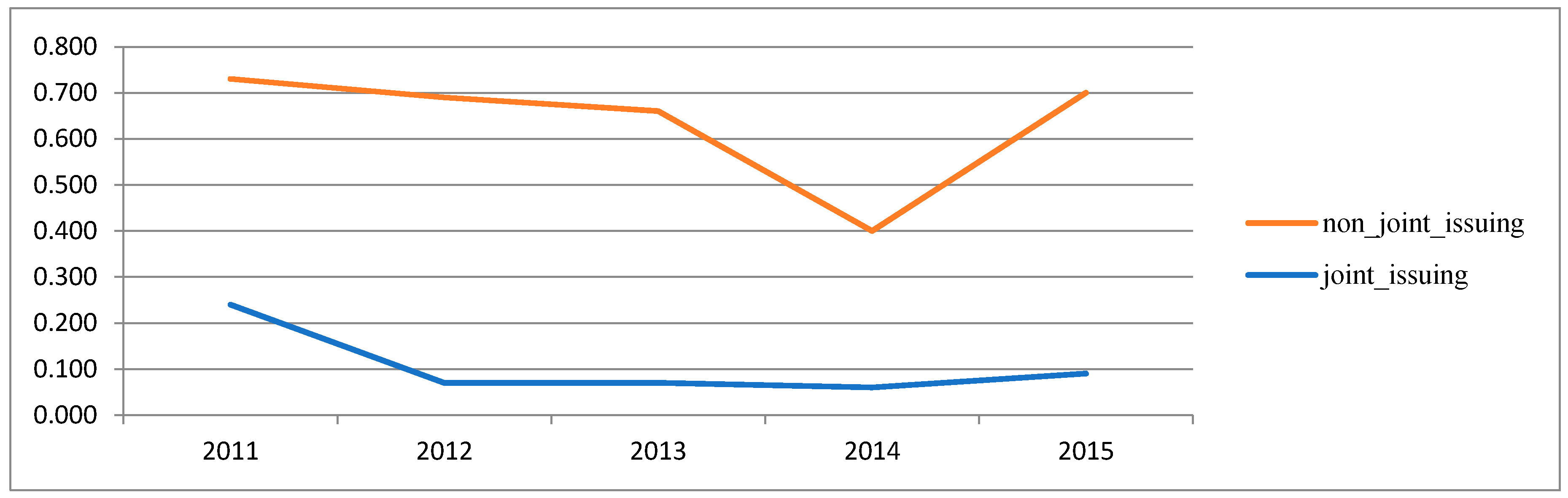
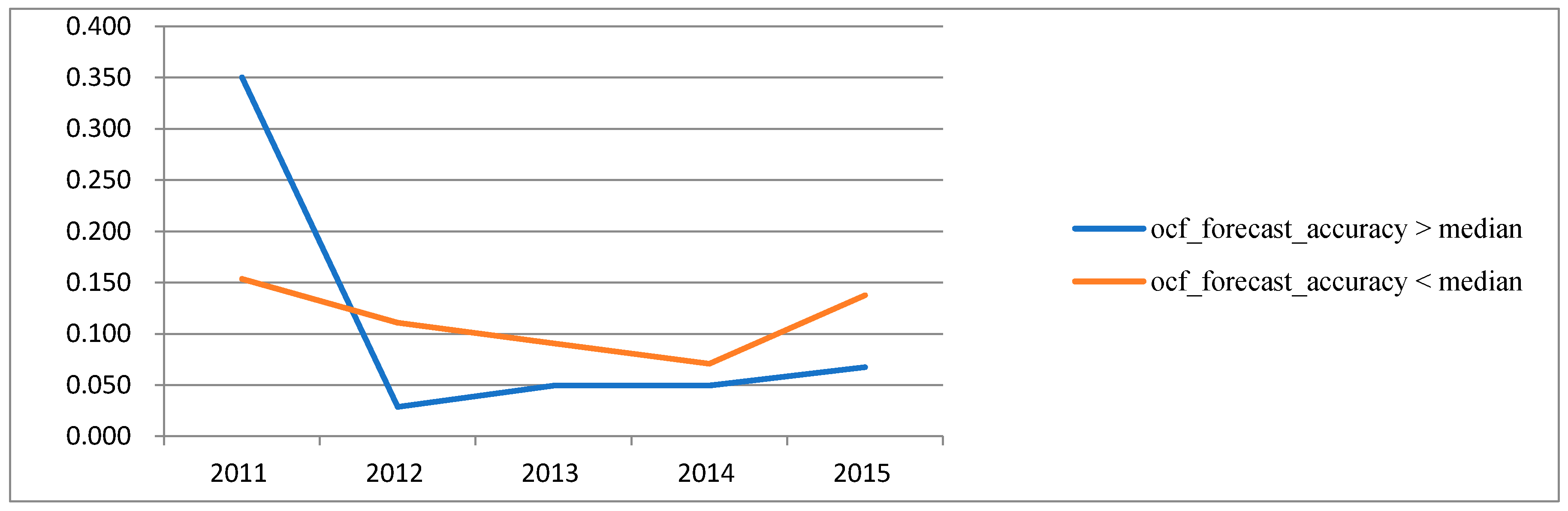
Table 4 shows Analysts’ Earnings Forecasts Error by year for H 1-1.Figure 1 depicts analysts’ earnings forecast by year for the sample of Hypothesis 1-1. We measure forecast error as the absolute value of the analysts’ earnings forecasts per share minus the actual earnings per share divided by the lagged stock price for firm i in year t. The variable joint_issuing represents the firm that simultaneously provided the financial analyst earnings forecast and the cash flow forecast. The variable non_joint_issuing represents the firm that provided only financial analyst earnings forecasts. Panel A shows the financial analysts’ forecast error of the firms that provided only the earnings forecasts compared to the simultaneously provided firms was larger. Table 5 shows Analysts’ Earnings Forecasts Error by year for H 1-2. Figure 2 depicts analysts’ earnings forecast by year for the sample of Hypothesis 1-2. The variable ocf_forecast_accuracy represents the accuracy of financial analyst cash flow forecast. Figure 1 shows the higher the accuracy of the cash flow forecast, the higher the earnings forecast. Exceptionally, the higher the accuracy of cash flow forecasts in 2011, the lower the accuracy of earnings forecasts. This can be interpreted as reflecting the financial analysts’ difficulty in estimating earnings from the adoption of K-IFRS from 2011.
4.2. Pearson Correlations
The Panel A of Table 6 shows the results of Pearson correlations of major variables for full samples. Financial analysts’ cash flow forecast dummy variables (JOINT_DUM), financial analysts’ coverage (FOLLOWS), profitability (ROE), and firm size (SIZE) show a significant positive correlated with financial analysts’ earnings forecast accuracy (AF_ACC) at 1%. This means that financial analysts’ earnings forecasts are more accurate for firms with the financial analyst earnings forecast and the cash flow forecast coexist, the higher the number of financial analysts, the higher the profitability, the larger the firm size. The debt ratio (LEV) and loss firms’ dummy variable (LOSSDUM) show a significant negative correlated with financial analysts’ earnings forecast accuracy (AF_ACC) at 1%. This means that financial analysts’ earnings forecasts are less accurate for firms with the higher the debt ratio, negative earnings. As correlation results do not control for differences in firm, industry characteristics, we now turn to multivariate tests.
The Panel B of Table 6 presents Pearson correlations for firms with analysts’ cash flow forecast data. Financial analysts’ cash flow forecast accuracy (OCF_ACC), financial analysts coverage (FOLLOWS), profitability (ROE) show a significant positive correlated with financial analysts’ earnings forecast accuracy (AF_ACC) at 1%. This means that financial analysts’ earnings forecasts are more accurate for firms with the higher financial analysts’ cash flow forecast accuracy, the higher the number of financial analysts, the higher the profitability. The debt ratio (LEV), loss dummy variable (LOSSDUM), listed years (AGE) and total asset growth rate (GRW) show a significant negative correlated with financial analysts’ earnings forecast accuracy (AF_ACC) at 1%. This means that financial analysts’ earnings forecasts are less accurate for firms with the higher the debt ratio, the loss firms, the longer the listing period, and the larger the total asset growth rate. As correlation results do not control for differences in firm, industry characteristics, we now turn to multivariate tests.
The Panel C of Table 6 shows the results of Pearson correlations of major variables for Hypothesis 2. Financial analysts’ cash flow forecast dummy variable (JOINT_DUM), standard deviation of daily return (STDRET), terminal price (PRICE), firm size (SIZE), systematic risk (BETA), and debt ratio (LEV) shows a negative relationship with information asymmetry (SPREAD) at 1%. This means that information asymmetry reduces for firms with the financial analyst earnings forecast and the cash flow forecast coexist, the higher the standard deviation of daily returns, the higher the terminal price, the larger the firm size, the systematic risk, the higher the foreign ownership and debt ratio. As correlation results do not control for differences in firm, industry characteristics, we now turn to multivariate tests.
4.3. Multivariate Results
[Model 1] to [Model 4] of Table 7 show the regression analysis of Hypothesis 1-1 for joint issuance and earnings forecast accuracy. As a result of the regression analysis, the F value is significant at the 1% level, so the regression model is appropriate. The variance expansion index (VIF) of the independent variable used in the regression analysis of this study was less than 2 and not more than 10, indicating that the problem of multicollinearity is not serious. The regression coefficient () of JOINT_DUM, which shows the relationship between joint issuance and earnings forecast accuracy, was 0.321, 0622, 0.212 and 0.142, which was a significant positive value at 1% level, respectively. The empirical results show that the financial analysts are more accurate in predicting earnings for a given firm when both earnings forecasts and cash flow forecasts are provided at the same time. These results show that the analysts who provide financial analysts’ earnings forecasts and cash flow forecasts simultaneously have more structured and accurate forecasts when financial analysts estimate earnings forecasts, which supports Hypothesis 1-1 [11].
[Model 1] to [Model 4] of Table 8 show the results of regression analysis of Hypothesis 1-2 for cash flow forecast accuracy and earnings forecast accuracy for firms that provided simultaneously. As a result of the regression analysis, the F value is significant at the 1% level, so the regression model is appropriate. The regression coefficient () of OCF_ACC, which indicates the relationship between cash flow forecast accuracy and earnings forecast accuracy, was 0.059, 0.059, 0.061 and 0.094, which was a significant positive value at 1% level, respectively. In other words, the empirical results show that the firm that accurately predicts the cash flow forecasts has higher accuracy of the analysts’ earnings forecasts than those that do not. These results show that the more accurately the cash flow forecast is estimated, the higher the earnings forecast accuracy is, and the better the cash flow forecast quality is, the more accurate the earnings forecast, which supports Hypothesis 1-2 [11].
[Model 1] to [Model 4] of Table 9 show the results of regression analysis of Hypothesis 2, which verified the relationship between joint issuance and information asymmetry. As a result of the regression analysis, the F value is significant at the 1% level, so the research model is appropriate. The variance expansion index (VIF) of the independent variables used in the regression analysis of this study was less than 2 and did not exceed 10. This means that the problem of multicollinearity is not serious. The regression coefficient () of JOINT_DUM of [Model 1], which indicates the relationship between joint issuance and information asymmetry, is −0.165, which is a significant negative value at 5% level. The regression coefficient () of JOINT_DUM of [Model 2] and [Model 3], which indicates the relationship between joint issuance and information asymmetry, is −0.232 and −0.256, which is a significant negative value at 1% level, respectively. The regression coefficient () of JOINT_DUM of [Model 4], which indicates the relationship between joint issuance and information asymmetry, is −0.210, which is a significant negative value at 10% level. In other words, firms that provide both earnings forecasts and cash flow forecasts show lower information asymmetry than firms that do not. These results show that firms providing both earnings forecasts and cash flow forecasts have more financial analysts than firms that do not provide both forecasts and cash flow forecasts, and the more financial analysts can provide a richer information environment, the less information asymmetry between managers and investors, which supports Hypothesis 2 [23].
5. Additional Tests
5.1. Sample Selection Bias
This section deals with the problem of sample selection bias related to the joint issuance of financial analysts’ earnings forecasts and cash flow forecasts. Since the problem of sample selection bias related to the joint issuance of financial analysts’ earnings forecasts and cash flow forecasts could have a potential impact on the results of this study, the two-step estimation model proposed by Heckman [46].
The first-order regression model variables that are expected to influence the selection of the joint issuance of financial analysts’ earnings forecasts and cash flow forecasts are as follows. Accruals (ACCRUAL), earnings volatility (VOL), business cycle (CYCLE), capital intensity (CAPINT), financial health (K1_SCORE), firm size (SIZE), earnings quality (EQ) [9,15,16,28]. The first-order regression model is as follows.
where JOINT_DUM: joint issuance dummy variable, an indicator variable equal to one if the financial analyst has provided both earnings and cash flow forecasts in a given year, 0 otherwise. ACCRUAL is absolute value of total accruals, which is measured as net income minus operating cash flow and standardized by total asset. VOL is earnings volatility and CYCLE is business cycle. CAPINT is capital intensity and K1_SCORE is financial health. SIZE is firm size, which is measured logarithm of total assets in year t-1. EQ is earnings quality, which is measured the absolute value of the residual estimated by the modified Jones model.
Inverse Mill’s Ratio (IMR) was estimated based on the above Probit model. The second regression model was analyzed by further controlling the estimated IMR. Table 10 shows the results of the regression analysis that re-verifies Hypothesis 1-1 about joint issuance and earnings forecast accuracy by controlling sample selection bias. As a result of the regression analysis, the F value is significant at the 1% level, so the research model is appropriate. The regression coefficient () of JOINT_DUM, which indicates the relationship between the joint issuance and the earnings forecast accuracy, was 0.363, which was a significant positive value at the 1% level. Therefore, this suggest that the analysts who provide both the earnings forecasts and the cash flow forecasts are more accurate than the analysts who provide only the earnings forecasts. Additionally, the results of this study show that the analysts who provide both financial analyst earnings forecasts and cash flow forecasts can make more structured and accurate forecasts when financial analysts estimate earnings forecasts [11].
Table 11 shows the results of the regression analysis that re-verifies Hypothesis 2 for joint issuance and information asymmetry by controlling sample selection bias. As a result of the regression analysis, the F value is significant at the 1% level, so the research model is appropriate. The regression coefficient () of JOINT_DUM, which indicates the relationship between the joint issuance and the information asymmetry, was −0.138, which was a significant negative value at the 10% level. Therefore, firms that provide both earnings forecasts and cash flow forecasts show lower information asymmetry than firms that do not. These results support Hypothesis 2, which shows that firms that provide both earnings forecasts and cash flow forecasts have more financial analysts and that more financial analysts’ followings can reduce information asymmetry between managers and investors based on rich information environment [23].
5.2. Re-Verification after Controlling the Time Series and Cross-Sectional Dependency
Table 12 shows the results of the regression analysis of Hypothesis 1-1 for joint issuance and earnings forecast accuracy by modifying the t-value with the methodology of Gow et al. [47] to control time series dependency and cross-sectional dependency. The regression coefficient () of JOINT_DUM, which shows the relationship between joint issuance and earnings forecast accuracy, was 0.368, which was a significant positive value at 1% level. The empirical results show that the financial analysts are more accurate in predicting earnings for a given firm when both earnings forecasts and cash flow forecasts are provided at the same time. These results show that the analysts who provide financial analyst earnings forecasts and cash flow forecasts simultaneously have more structured and accurate forecasts when financial analysts estimate earnings forecasts, which supports Hypothesis 1-1 [11].
Table 13 shows the results of the regression analysis of Hypothesis 1-2 by modifying the t-value with the methodology of Gow et al. [47] to control time series dependency and cross-sectional dependency. The regression coefficient () of OCF_ACC, which indicates the relationship between cash flow forecast accuracy and earnings forecast accuracy was 0.046, which was a significant positive value at 5% level. In other words, the empirical results show that the firm that accurately predicts the cash flow forecasts has higher accuracy of the analysts’ earnings forecasts than those that do not. These results show that the more accurately the cash flow forecast is estimated, the higher the earnings forecast accuracy is, and the better the cash flow forecast quality is, the more accurate the earnings forecast, which supports Hypothesis 1-2 [11].
Table 14 shows the results of the regression analysis of Hypothesis 2 by modifying the t-value with the methodology of Gow et al. [47] to control time series dependency and cross-sectional dependency. As a result of the regression analysis, the F value is significant at the 1% level, so the research model is appropriate. The regression coefficient () of JOINT_DUM, which indicates the relationship between joint issuance and information asymmetry, was −0.142, indicating negative direction but not significant.
6. Conclusions
This study empirically analyzes whether cash flow forecasting information provided by financial analysts increases firm transparency and sustainability by reducing information asymmetry between investors and stakeholders. Financial analysts have provided a variety of information as information intermediary in the capital markets. The information provided by financial analysts includes earnings forecast information, sales forecast information, target price, and stock recommendation. The information they provide has been verified in several previous studies as contributing to making capital markets more efficient by mitigating conflicting interests among stakeholders in the capital market [3,26,48]. Financial analysts have recently provided additional cash flow forecasts. After DeFond and Hung [9], the first study on why analysts provide cash flow forecasts, a variety of studies have been conducted on analysts’ cash flow forecasts. The majority of studies have focused on the assumption that investors demand cash flow forecasts when the quality of earnings is low, according to DeFond and Hung [9]. However, the question of information usefulness of cash flow forecasts and the consideration from suppliers that provide information are also being studied continuously. For example, there are determinants of financial analyst cash flow forecasts from suppliers’ perspective [18], the impact of cash flow forecasts on management reporting and the price formation of investors in earnings [10,28], the relative accuracy of earnings forecasts when cash flow forecasts exist [11], market response when financial analysts meet cash flow forecasts [13], and the determination of the accuracy of cash flow forecasts [21,49].
The above studies indirectly suggest evidence that financial analysts’ cash flow forecasts are meaningful to investors and that financial analysts are helpful for their own earnings forecasts. On the other hand, Givoly et al. [14] concluded that financial analysts’ cash flow forecasts are simply computed by adding the depreciation cost to the earnings forecasts, and are thus lacking in sophistication. In addition, Blinski [15] argues that financial analysts who provide forecasting information do not provide cash flow forecasts for firms with low-quality earnings because firms with low profitability may suffer from their reputation and earnings by reporting the results; Blinski [15] presented a supplier perspective. Therefore, although there are various studies on cash flow forecasts of financial analysts abroad, there are few studies in Korea yet. In this paper, we analyze the information usefulness of analysts’ cash flow forecasts in the Korean environment, which is different from the US capital market environment and accounting transparency.
The empirical results of this study are as follows. First, the effect of joint issuance of financial analysts’ earnings forecasts and cash flow forecasts on the accuracy of earnings forecasts is significantly positive. Therefore, firms that provide both earnings forecasts and cash flow forecasts are more likely to predict earnings analysts’ earnings accuracy than those that do not. The effect of financial analysts’ cash flow forecast accuracy on the accuracy of earnings forecasts is significantly positive. Therefore, the empirical results show that firms that accurately predicted cash flow forecasts have higher earnings forecasting accuracy than those that do not. Second, the joint issuance of financial analysts’ earnings forecasts and cash flow forecast on bid–ask spreads are significant negative. These results show that the information asymmetry between the manager and the investor can be reduced based on the rich information environment. Additionally, financial analysts’ cash flow forecasting information is expected to increase corporate transparency and sustainability by reducing information asymmetry between manager and investors.
The contributions of this study are as follows. First, this study comprehensively reviewed the usefulness of cash flow forecasts of financial analysts. The study on the cash flow forecast of financial analysts is actively conducted outside of the country, but the research has not yet been conducted in Korea. In this situation, it is meaningful to analyze the relationship between cash flow forecasts and earnings forecasts, the usefulness of cash flow forecasts, and the information environment on the basis of Korean data. Second, earnings forecasts and cash flow forecasts provided by financial analysts were data on individual financial statements until the introduction of K-IFRS. However, since K-IFRS was adopted, financial analysts mainly provide forecasts for consolidated financial statements as their main financial statements have changed to consolidated financial statements. This study is different from the previous studies in data for consolidated financial statements. Third, the study of financial analysts’ cash flow forecasts has mainly been centered on the United States. The legal origins of the US and Korea are different, and the effects of financial analyst activity on the capital market are expected to be discriminatory. In this study, it is meaningful to directly examine the influence of financial analysts and capital markets in the Korean environment under a different legal basis from the United States. Fourth, the accounting environments in Korea and the US are very different. In such accounting environments, the role of financial analysts in the capital market may become even more important. It is significant that this study further analyzed and interpreted the usefulness of cash flow forecasts provided by financial analysts in a different accounting environment than in the United States. Fifth, this study is expected to provide important implications for capital market participants in that the analysts’ cash flow forecasts provide evidence that capital market participants’ information can be used as useful information for economic decision-making.
The limitations of this study are as follows. First, there may be a problem of omitted variables that may further affect the financial analysts’ earnings forecasts, earnings quality, and the information environment. Second, there may be a measurement error in estimating variables such as earnings quality and information asymmetry. Third, the informativeness of cash flow forecasts might be different because forecasts are issued by different kind of analysts. To issue cash flow forecasts requires more effort. Analysts with high ability might be more likely to issue cash flow forecasts. It may not cash flow forecasts contribute to the reduction of information asymmetry. The reduction of information asymmetry results from firms covered by more good analysts. In this study, consensus of financial analysts is set as a variable of interest to minimize such convenience. We believe that the convenience of individual financial analysts based on their abilities can be controlled to some extent by using consensus. In addition, it would be very interesting to review the usefulness of the information provided by individual financial analysts in future studies. Fourth, Heckman’s [1] methodology was used to control the selection bias for firms that simultaneously provide financial analyst earnings forecasts and cash flow forecasts. However, there are still few studies on the incentives of joint issuance. Since supplier perspectives are also relevant in this area of research, further work will be conducted so that various simultaneous incentives can be considered in the future.
Author Contributions
Conceptualization, H.M.O.; Investigation, H.M.O. and H.Y.S; Methodology, H.M.O.; Supervision, H.Y.S; Writing—original draft, H.M.O.; Writing—review & editing, H.Y.S.
Funding
This research received no external funding.
Conflicts of Interest
The authors declare no conflict of interest.
Appendix A. Variable Definitions for H1-1, H1-2, H2
Appendix A.1. Dependent Variables
| AF_ACC | financial analysts’ earnings forecast accuracy, -1*| analysts’ earnings forecast per share – actual earnings per share | / lagged stock price for firm i in year t |
| SPREAD | Iinformation asymmetry, spread according to Corwin and Schultz [35] for firm i in year t |
Appendix A.2. Explanatory Variables
| JOINT_DUM | joint issuance dummy variable, an indicator variable equal to one if the financial analyst has provided both earnings and cash flow forecasts in a given year, 0 otherwise |
| OCF_ACC | financial analysts’ cash flow forecasts accuracy, −1*| analysts’ cash flow forecasts per share – actual cash flow per share | / lagged stock price for firm i in year t |
Appendix A.3. Control Variables
| EQ | the absolute residual of the Dechow et al. [50]. discretionary accrual model, multiplied by −1; |
| FOLLOWS | the number of analysts who report earnings forecasts for the firm; |
| LEV | financial leverage, measured as long-term liabilities divided by lagged total assets; |
| ROE | return on equity, measured as net income divided by lagged total equity; |
| SIZE | firm size, the natural log of total assets; |
| AGE | the number of years from the date of initial listing to the lagged period; |
| GRW | asset growth, measured as the total assets in year t minus total assets in t−1 divided by total assets in t−1; |
| STDRET | standard deviation of daily returns |
| PRICE | the natural log of closing price at the end of March for firm i in year t+1 |
| BETA | systematic risk, estimated value using monthly stock returns for firm i over the five years period from year t to year t-4 |
| FOR | foreign ownership |
| YD | year dummy; |
| IND | industry dummy. |
Appendix A.4. Variable Definitions for Probit Model
| JOINT_DUM | joint issuance dummy variable, an indicator variable equal to one if the financial analyst has provided both earnings and cash flow forecasts in a given year, 0 otherwise |
| ACCRUAL | absolute value of total accruals, measured as absolute value of net income minus operating cash flow divided by total assets in t; |
| VOL | earnings volatility, (standard deviation of earnings from year t-4 to year t / average deviation of earnings from year t-4 to year t) / (standard deviation of operating cash flow from year t-4 to year t / average deviation of operating cash flow from year t-4 to year t); |
| CYCLE | business cycle, 365/ inventory turnover + 365/ receivable turnover . where inventory turnover is measured as cost of goods sold divided average inventory and receivable turnover is measured as sales divided average receivable; |
| CAPINT | capital intensity, (gross property , plant and equipment) / sales; |
| K1_SCORE | financial health, K1-SCORE = −17.862+1.472X1+3.041X2+14.839X3+1.516X4 where, X1: natural logarithm of total assets X2: natural logarithm of (sales / total asset) X3: retained earnings / total asset X4: equity /debt |
| SIZE | firm size, logarithm of total assets in year t-1; |
| EQ | the absolute residual of the Dechow et al. [50]. discretionary accrual model, multiplied by −1. |
Appendix B. SPREAD is Measured as Corwin and Schultz (2012)
In this study, we use the following spreads estimated by Corwin and Schultz [35] using daily maximum and minimum prices. Corwin and Schultz [35] estimates can significantly reduce missing values in that they use daily stock prices, and it is advantageous to include corporate spreads throughout the day because they use the highest and lowest prices [51].
where is highest prices for firm in day t and is lowest prices for firm in day t; is highest prices for firm in day t+1 and is lowest prices for firm in day t + 1; is highest prices for firm in day and in day t + 1 and is lowest prices for firm in day and in day t + 1.
References
- Jain, P.K.; Rezaee, Z. The Sarbanes–oxley act of 2002 and capital-market behavior: Early evidence. Contemp. Account. Res. 2006, 23, 629–654. [Google Scholar] [CrossRef]
- Schipper, K. Commentary on earnings management. Account. Horiz. 1989, 3, 91–102. [Google Scholar]
- Healy, P.; Palepu, K. Information asymmetry, corporate disclosure, and the capital markets: A review of the empirical disclosure literature. J. Account. Econ. 2001, 31, 405–440. [Google Scholar] [CrossRef]
- Dyck, A.; Morse, A.; Zingales, L. Who blows the whistle on corporate fraud? J. Financ. 2010, 65, 2213–2253. [Google Scholar] [CrossRef]
- Yu, F. Analyst coverage and earnings management. J. Financ. Econ. 2008, 88, 245–271. [Google Scholar] [CrossRef]
- Knyazeva, D. Corporate Governance, Analyst Following, and Firm Behaviour; Working Paper; New York University: New York, NY, USA, 2014 2007; Available online: http://www.efmaefm.org/0EFMAMEETINGS/EFMA%20ANNUAL%20MEETINGS/2008-Athens/papers/Diana.pdf (accessed on 18 June 2019).
- Sun, J. Governance role of analyst coverage and investor protection. Financ. Anal. J. 2009, 65, 52–64. [Google Scholar] [CrossRef]
- Sun, J.; Liu, G. The effect of analyst coverage on accounting conservatism. Manag. Financ. 2011, 37, 5–20. [Google Scholar] [CrossRef] [Green Version]
- Defond, M.L.; Hung, M. An empirical analysis of analysts’ cash flow forecasts. J. Account. Econ. 2003, 35, 73–100. [Google Scholar] [CrossRef]
- McInnis, J.; Collins, D. The effect of cash flow forecasts on accrual quality and benchmark beating. J. Account. Econ. 2011, 51, 219–239. [Google Scholar] [CrossRef]
- Call, A.C.; Chen, S.; Tong, T.H. Are analysts’ earnings forecasts more accurate when accompanied by cash flow forecasts? Rev. Account. Stud. 2009, 14, 358–391. [Google Scholar] [CrossRef]
- Call, A.C.; Chen, S.; Tong, Y.H. Are analysts’ cash flow forecasts naïve extensions of their own earnings forecasts? Contemp. Account. Res. 2013, 30, 438–465. [Google Scholar] [CrossRef]
- Brown, L.D.; Huang, K.; Pinello, A.S. To beat or not to beat? The importance of analysts’ cash flow forecasts. Rev. Quant. Financ. Account. 2013, 41, 723–752. [Google Scholar] [CrossRef]
- Givoly, D.; Hayn, C.; Lehavy, R. The quality of analysts’ cash flow forecasts. Account. Rev. 2009, 84, 1877–1911. [Google Scholar] [CrossRef]
- Bilinski, P. Do analysts disclose cash flow forecasts with earnings estimates when earnings quality is low? J. Bus. Financ. Account. 2014, 41, 401–434. [Google Scholar] [CrossRef]
- Defond, M.L.; Hung, M. Investor protection and analysts’ cash flow forecasts around the world. Rev. Account. Stud. 2007, 12, 377–419. [Google Scholar] [CrossRef]
- Ahmed, K.; Ali, M.J. Determinants and usefulness of analysts’ cash flow forecasts: Evidence from Australia. Int. J. Account. Inf. Manag. 2013, 21, 4–21. [Google Scholar] [CrossRef]
- Ertimur, Y.; Stubben, S. Analysts’ incentives to issue revenue and cash flow forecasts. Working paper. Duke University and University of North Carolina at Chapel Hill. SSRN Electron. J. 2005, 1–51. [Google Scholar] [CrossRef]
- Shin, H.; Oh, H. Earnings quality and the joint issuance of analyst earnings and cash flow forecasts. Account. Inf. Res. 2014, 32, 113–137. [Google Scholar]
- Christopher, T.; Edmonds, J.E.E.; Maher, J.J. The impact of meeting or beating analysts’ operating cash flow forecasts on a firm’s cost of debt. Adv. Account. 2011, 27, 242–255. [Google Scholar] [CrossRef]
- Pae, J.; Yoon, S. Determinants of analysts’ cash flow forecast accuracy. J. Account. Audit. Financ. 2011, 27, 123–144. [Google Scholar] [CrossRef]
- Gordon, E.A.; Petruska, K.A.; Yu, M. Do analysts‘ cash flow forecasts mitigate the accrual anomaly? International evidence. J. Int. Account. Res. 2014, 13, 61–90. [Google Scholar] [CrossRef]
- Dhole, S.; Mishra, S.; Pal, A.M. Are Analysts’ Cash Flow Forecasts Important? Another Examination; Working Paper; University of Melbourne: Melbourne, Australia, 2014; pp. 1–40. [Google Scholar]
- Shi, L.; Zhang, H.; Guo, J. Analyst cash flow forecasts and pricing of accruals. Adv. Account. Inc. Adv. Account. 2014, 30, 95–105. [Google Scholar] [CrossRef]
- Mao, M.Q.; Yu, Y. Analysts’ cash flow forecasts, audit effort, and audit opinions on internal control. J. Bus. Financ. Account. 2015, 42, 635–664. [Google Scholar] [CrossRef]
- Song, M.S. Do Analysts use the Cash Flow Forecasts for Stock Recommendation? Korean Account. Rev. 2015, 40, 83–118. [Google Scholar]
- Hyeon, J.W.; Kim, Y.J.; Lee, J.I. Analysts’ operating cash flow forecasts and accuracy of earnings forecasts: Korean evidence. Study Account. Tax. Audit. 2016, 69, 221–253. [Google Scholar]
- Call, A.C. Analysts’ cash flow forecasts and the predictive ability and pricing of operating cash flows. Working paper. University of Georgia. SSRN Electron. J. 2008, 1–50. [Google Scholar] [CrossRef]
- Hirshleifer, D.; Teoh, S.H. Limited attention, information disclosure, and financial reporting. J. Account. Econ. 2003, 36, 337–386. [Google Scholar] [CrossRef]
- Givoly, D.; Hayn, C.; Lehavy, R. Analysts’ cash flow forecasts are not sophisticated: A rebuttal of call, chen and tong. SSRN Electron. J. 2013, 1–7. [Google Scholar] [CrossRef]
- Mohanram, P.S. Analysts’ cash flow forecasts and the decline of the accruals anomaly. Contemp. Account. Res. 2014, 31, 1143–1170. [Google Scholar] [CrossRef]
- Radhakrishnan, S.; Wu, S.L. Analysts’ cash flow forecasts and accrual mispricing. Contemp. Account. Res. 2014, 31, 1191–1219. [Google Scholar] [CrossRef]
- Jeong, S.W. Factors associated with analyst following and forecast characteristics. Korean Account. Rev. 2003, 28, 61–84. [Google Scholar]
- Bae, K.S.; Park, M.H. The effect of asset impairments on effective Analyst’s earnings forecast error and accuracy. Korean Account. J. 2011, 20, 1–27. [Google Scholar]
- Corwin, S.A.; Schultz, P. A simple way to estimate bid-ask spreads from daily high and low prices. J. Financ. 2012, 67, 719–760. [Google Scholar] [CrossRef]
- Shin, S.N. The Effect of K-IFRS Adoption on Information Asymmetry and Stock Price Synchronicity. Ph.D. Thesis, Sungkyunkwan University, Seoul, Korea, 2013. Available online: http://www.riss.kr/search/detail/DetailView.do?p_mat_type=be54d9b8bc7cdb09&control_no=2e5452a78a173652ffe0bdc3ef48d419 (accessed on 18 June 2019).
- Park, J.H.; Cho, J.S. The Effects of corporate governance characteristics on information asymmetry and stock price synchronicity. Korean Account. Rev. 2015, 40, 285–325. [Google Scholar]
- Oh, H.M.; Shin, H.Y. Voluntary disclosure, information asymmetry and corporate governance after the adoption of IFRS. Account. Inf. Res. 2016, 34, 159–188. [Google Scholar]
- Cho, J.S.; Jo, M.H. The Effect of accrual volatility on the firms’ information asymmetry, forecast error, and cost of capital. Korean Account. J. 2010, 19, 175–199. [Google Scholar]
- Francis, J.; LaFond, R.; Olsson, P.; Schipper, K. The market pricing of accruals quality. J. Account. Econ. 2005, 39, 295–327. [Google Scholar] [CrossRef]
- Botosan, C.A. Disclosure level and the cost of equity capital. Account. Rev. 1997, 72, 323–349. [Google Scholar]
- Ahn, Y.Y.; Shin, H.H.; Chang, J.H. The relationship between the foreign investor and information asymmetry. Korean Account. Rev. 2005, 30, 109–131. [Google Scholar]
- Glosten, L.R.; Harris, L.E. Estimating the components of the bid–ask spread. J. Financ. Econ. 1988, 21, 123–142. [Google Scholar] [CrossRef]
- Chang, H.S.; Ok, J.H. A study on the spread in the Korean stock market: An empirical analysis on the determinants and the behavior in the day. Asian Rev. Financ. Res. 1996, 11, 21–63. [Google Scholar]
- Jang, S.O. Information asymmetry and earnings management. Account. Inf. Res. 2007, 25, 221–245. [Google Scholar]
- Heckman, J.J. Sample selection bias as a specification error. Econometrica 1979, 47, 153–161. [Google Scholar] [CrossRef]
- Gow, I.D.; Ormazabal, G.; Taylor, D.J. Correcting for cross–sectional and time–series dependence in accounting research. Account. Rev. 2010, 85, 483–512. [Google Scholar] [CrossRef]
- Choi, S.U.; Lee, W.J. Analyst coverage and corporate investment efficiency. J. Ind. Econ. Bus. 2015, 28, 317–336. [Google Scholar]
- Yoo, C.Y.; Pae, J. Estimation and prediction tests of cash flow forecast accuracy. J. Forecast. 2011, 32, 215–225. [Google Scholar] [CrossRef]
- Dechow, P.M.; Sloan, R.G.; Sweeney, A.P. Detecting Earnings Management. Account. Rev. 1995, 70, 193–225. [Google Scholar]
- Cheong, E.H.; Woo, Y.S. The effect of K-IFRS adoption on bid–ask spread: The discriminatory effect by firm’s characteristics. Account. Inf. Res. 2015, 33, 211–236. [Google Scholar]
Figure 1.
Analysts’ earnings forecasts error by year H 1-1.

Figure 2.
Analysts’ earnings forecasts error by year for H 1-2.


Table 1.
Sample selection.
| Criteria | Firm-Year Observations |
|---|---|
| Quoted firms for fiscal years 2011–2015 | 3508 |
| (less) non-December 31 firms and financial firms for fiscal years | (308) |
| (less) Firms for which financial and stock data cannot be collected from FN-Guide and TS-2000 | (626) |
| (less) Firms for which analysts’ forecast data cannot be collected from FN-Guide | (1594) |
| Final sample | 980 |
Table 2.
Distributions over the sample period.
| Panel A: Distribution Across Fiscal Years | ||||||
| Year | N | Firms with Analysts’ Cash Flow Forecasts Data | Percent (%) | Firms without Analysts’ Cash Flow Forecasts Data | Percent (%) | |
| 2011 | 109 | 67 | 61.47 | 42 | 38.53 | |
| 2012 | 142 | 131 | 92.25 | 11 | 7.75 | |
| 2013 | 215 | 175 | 81.40 | 40 | 18.60 | |
| 2014 | 240 | 200 | 83.33 | 40 | 16.67 | |
| 2015 | 274 | 263 | 95.99 | 11 | 4.01 | |
| Total | 980 | 836 | 85.31 | 144 | 14.69 | |
| Panel B: Industry Distribution | ||||||
| Industry | N | Firms with Analysts’ Cash Flow Forecasts Data | Percent (%) | Firms without Analysts’ Cash Flow Forecasts Data | Percent (%) | |
| Food, Beverage | 61 | 56 | 91.80 | 5 | 8.20 | |
| Fiber, Clothes, Leathers | 35 | 31 | 88.57 | 4 | 11.43 | |
| Timber, Pulp, Furniture | 11 | 8 | 72.73 | 3 | 27.27 | |
| Cokes, Chemical | 119 | 102 | 85.71 | 17 | 14.29 | |
| Medical Manufacturing | 36 | 31 | 86.11 | 5 | 13.89 | |
| Rubber & Plastic | 27 | 23 | 85.19 | 4 | 14.81 | |
| Non-Metallic | 14 | 9 | 64.29 | 5 | 35.71 | |
| Metallic | 52 | 42 | 80.77 | 10 | 19.23 | |
| Pc, Medical | 63 | 57 | 90.48 | 6 | 9.52 | |
| Machine & Electronic | 58 | 47 | 81.03 | 11 | 18.97 | |
| Other Transportation | 83 | 71 | 85.54 | 12 | 14.46 | |
| Construction | 52 | 44 | 84.62 | 8 | 15.38 | |
| Retail & Whole Sales | 95 | 84 | 88.42 | 11 | 11.58 | |
| Transportation Service | 35 | 30 | 85.71 | 5 | 14.29 | |
| Publishing, Broadcasting | 40 | 34 | 85.00 | 6 | 15.00 | |
| Professional Services | 104 | 88 | 84.62 | 16 | 15.38 | |
| Other | 95 | 79 | 83.16 | 16 | 16.84 | |
| Total | 980 | 836 | 85.31 | 144 | 14.69 | |
Table 3.
Descriptive statistics.
| PANEL A (N = 980) Full Sample for H 1-1 | |||||||
| Variable | Mean | Std. Dev. | Min | 25th Percentile | Median | 75th Percentile | Max |
| AF_ACC | −0.151 | 0.286 | −0.941 | −0.092 | −0.033 | −0.011 | 0.000 |
| JOINT_DUM | 0.853 | 0.354 | 0.000 | 1.000 | 1.000 | 1.000 | 1.000 |
| FOLLOW | 7.879 | 7.767 | 1.000 | 1.000 | 4.000 | 13.000 | 27.000 |
| LEV | 0.499 | 0.188 | 0.121 | 0.345 | 0.520 | 0.633 | 0.906 |
| ROE | 0.065 | 0.221 | −0.582 | 0.028 | 0.074 | 0.124 | 0.329 |
| SIZE | 28.484 | 1.593 | 25.507 | 27.214 | 28.324 | 29.619 | 32.623 |
| LOSSDUM | 0.149 | 0.356 | 0.000 | 0.000 | 0.000 | 0.000 | 1.000 |
| AGE | 2.697 | 0.895 | 0.000 | 2.079 | 2.890 | 3.367 | 4.094 |
| GRW | 0.185 | 0.707 | −0.717 | −0.060 | 0.045 | 0.157 | 1.944 |
| PANEL B (N = 836) Firm Samples with Analysts’ Cash Flow Forecasts Data | |||||||
| Variable | Mean | Std. Dev. | Min | 25th Percentile | Median | 75th Percentile | Max |
| AF_ACC | −0.092 | 0.194 | −0.941 | −0.069 | −0.026 | −0.009 | 0.000 |
| OCF_ACC | −0.186 | 0.235 | −1.417 | −0.213 | −0.115 | −0.060 | −0.006 |
| FOLLOW | 9.016 | 7.872 | 1.000 | 2.000 | 6.000 | 15.000 | 27.000 |
| LEV | 0.501 | 0.190 | 0.121 | 0.344 | 0.521 | 0.637 | 0.906 |
| ROE | 0.062 | 0.234 | −0.582 | 0.028 | 0.074 | 0.124 | 0.329 |
| SIZE | 28.647 | 1.572 | 25.507 | 27.388 | 28.582 | 29.782 | 32.623 |
| LOSSDUM | 0.152 | 0.359 | 0.000 | 0.000 | 0.000 | 0.000 | 1.000 |
| AGE | 2.713 | 0.879 | 0.000 | 2.079 | 2.890 | 3.401 | 4.094 |
| GRW | 0.180 | 0.653 | −0.717 | −0.036 | 0.049 | 0.148 | 1.944 |
| PANEL C (N = 144) Firm Samples with only Earnings Forecasts | |||||||
| Variable | Mean | Std. Dev. | Min | 25th Percentile | Median | 75th Percentile | Max |
| AF_ACC | −0.496 | 0.444 | −0.941 | −0.941 | −0.586 | −0.041 | −0.002 |
| FOLLOW | 1.324 | 0.735 | 1.000 | 1.000 | 1.000 | 1.000 | 7.000 |
| LEV | 0.487 | 0.178 | 0.121 | 0.361 | 0.495 | 0.616 | 0.850 |
| ROE | 0.067 | 0.127 | −0.716 | 0.028 | 0.074 | 0.132 | 0.312 |
| SIZE | 27.538 | 1.369 | 25.507 | 26.601 | 27.368 | 28.143 | 32.327 |
| LOSSDUM | 0.131 | 0.339 | 0.000 | 0.000 | 0.000 | 0.000 | 1.000 |
| AGE | 2.605 | 0.976 | 0.000 | 2.079 | 2.833 | 3.258 | 4.025 |
| GRW | 0.217 | 0.967 | −0.717 | −0.717 | −0.007 | 0.547 | 1.944 |
| PANEL D (N = 975) Sample for H 2 | |||||||
| Variable | Mean | Std. Dev. | Min | 25th Percentile | Median | 75th Percentile | Max |
| SPREAD | 0.806 | 0.515 | 0.000 | 0.407 | 0.650 | 1.186 | 1.830 |
| JOINT_DUM | 0.852 | 0.355 | 0.000 | 1.000 | 1.000 | 1.000 | 1.000 |
| STERET | 2.404 | 0.548 | 1.675 | 1.940 | 2.337 | 2.785 | 3.375 |
| PRICE | 10.582 | 1.441 | 6.397 | 9.445 | 10.556 | 11.495 | 14.639 |
| SIZE | 27.832 | 1.538 | 24.399 | 26.612 | 27.829 | 28.909 | 33.044 |
| BETA | 0.847 | 0.647 | −0.185 | 0.364 | 0.801 | 1.310 | 2.059 |
| FOR | 0.179 | 0.152 | 0.000 | 0.061 | 0.144 | 0.256 | 0.897 |
| LEV | 0.497 | 0.179 | 0.186 | 0.344 | 0.517 | 0.633 | 0.788 |
Notes: This table presents the descriptive statistics for the variables used in the regression analyses. AF_ACC is financial analysts’ earnings forecast accuracy, −1*| analysts’ earnings forecasts per share – actual earnings per share | / lagged stock price for firm i in year t; JOINT_DUM is joint issuance dummy variable, an indicator variable equal to one if the financial analyst has provided both earnings and cash flow forecasts in a given year, 0 otherwise; FOLLOWS is the number of analysts who report earnings forecasts for the firm; LEV is financial leverage, measured as long-term liabilities divided by lagged total assets; ROE is return on equity, measured as net income divided by lagged total equity; SIZE is firm size, the natural log of total assets; LOSSDUM is loss dummy variable, 1 if net income is negative, and 0 otherwise; AGE is the number of years from the date of initial listing to the lagged period; GRW is asset growth, measured as the total assets in year t minus total assets in t-1 divided by total assets in t-1; SPREAD is information asymmetry, spread according to Corwin and Schultz [35] for firm i in year t; STDRET is standard deviation of daily returns; PRICE is the natural log of closing price at the end of March for firm i in year t+1; BETA is systematic risk, estimated value using monthly stock returns for firm i over the five years period from year t to year t-4; FOR is foreign ownership.
Table 4.
Analysts’ Earnings Forecasts Error for H 1-1.
| Panel A | |||||
|---|---|---|---|---|---|
| Analysts’ Earnings Forecasts Error by Year (N = 980) for H 1-1 | |||||
| Variable | 2011 | 2012 | 2013 | 2014 | 2015 |
| joint_issuing | 0.240 | 0.070 | 0.070 | 0.060 | 0.090 |
| not_joint_issuing | 0.049 | 0.062 | 0.590 | 0.340 | 0.610 |
Table 5.
Analysts’ Earnings Forecasts Error for H 1-2.
| Panel A | |||||
|---|---|---|---|---|---|
| Analysts’ Earnings Forecasts Error by Year (N = 836) for H 1-2 | |||||
| Variable | 2011 | 2012 | 2013 | 2014 | 2015 |
| ocf_forecast_accuracy > median | 0.350 | 0.029 | 0.049 | 0.050 | 0.067 |
| ocf_forecast_accuracy < median | 0.154 | 0.111 | 0.091 | 0.071 | 0.138 |
Table 6.
Pearson correlations.
| Panel A | ||||||||
| JOINT_DUM | FOLLOW | LEV | ROE | SIZE | LOSSDUM | AGE | GRW | |
| AF_ACC | 0.505 *** | 0.269 *** | −0.135 *** | 0.244 *** | 0.165 *** | −0.217 *** | 0.020 | −0.067 |
| JOINT_DUM | 0.355 *** | 0.027 | 0.005 | 0.246 *** | 0.020 | 0.044 | −0.065 ** | |
| FOLLOW | 0.119 *** | 0.021 | 0.668 *** | 0.027 | 0.009 | −0.039 | ||
| LEV | −0.373 *** | 0.371 *** | 0.356 *** | 0.022 | 0.098 *** | |||
| ROE | −0.120 *** | −0.068 *** | −0.065 ** | 0.059 * | ||||
| SIZE | 0.152 *** | 0.201 *** | 0.266 *** | |||||
| LOSSDUM | 0.038 | 0.006 | ||||||
| AGE | −0.053 * | |||||||
| Panel B | ||||||||
| OCF_ACC | FOLLOW | LEV | ROE | SIZE | LOSSDUM | AGE | GRW | |
| AF_ACC | 0.135 *** | 0.144 *** | −0.217 *** | 0.407 *** | −0.015 | −0.366 *** | −0.073 ** | −0.088 ** |
| OCF_ACC | 0.004 | −0.101 *** | 0.197 *** | 0.008 | −0.117 *** | 0.058 * | −0.004 | |
| FOLLOW | 0.124 *** | 0.020 | 0.676 *** | 0.023 | −0.009 | −0.025 | ||
| LEV | −0.387 *** | 0.374 *** | 0.369 *** | 0.001 | 0.059 *** | |||
| ROE | −0.131 *** | −0.674 *** | −0.090 *** | 0.075 ** | ||||
| SIZE | 0.164 *** | 0.198 *** | 0.227 *** | |||||
| LOSSDUM | 0.053 | 0.001 * | ||||||
| AGE | −0.063 * | |||||||
| Panel C | ||||||||
| JOINT_DUM | STDRET | PRICE | SIZE | BETA | FOR | LEV | ||
| SPREAD | −0.111 *** | −0.094 *** | −0.082 *** | −0.358 | −0.289 *** | −0.125 *** | −0.240 *** | |
| JOINT_DUM | -0.085 *** | 0.191 *** | 0.287 *** | 0.039 | 0.198 *** | 0.023 | ||
| STDRET | −0.227 *** | −0.205 *** | 0.072 ** | −0.229 *** | 0.165 *** | |||
| PRICE | 0.660 *** | −0.081 *** | 0.407 *** | −0.176 *** | ||||
| SIZE | 0.058* | 0.576 *** | 0.023 | |||||
| BETA | −0.040 | 0.272 *** | ||||||
| FOR | −0.152 *** | |||||||
Notes: This table presents the Pearson correlations for the variables used in the regression analyses. AF_ACC is financial analysts’ earnings forecast accuracy, −1*| analysts’ earnings forecasts per share – actual earnings per share | / lagged stock price for firm i in year t; OCF_ACC is financial analysts’ cash flow forecast accuracy, −1*| analysts’ cash flow forecasts per share – actual cash flow per share | / lagged stock price for firm i in year t ; JOINT_DUM is joint issuance dummy variable, an indicator variable equal to one if the financial analyst has provided both earnings and cash flow forecasts in a given year, 0 otherwise; FOLLOWS is the number of analysts who report earnings forecasts for the firm; LEV is financial leverage, measured as long-term liabilities divided by lagged total assets; ROE is return on equity, measured as net income divided by lagged total equity; SIZE is firm size, the natural log of total assets; LOSSDUM is loss dummy variable, 1 if net income is negative, and 0 otherwise; AGE is the number of years from the date of initial listing to the lagged period; GRW is asset growth, measured as the total assets in year t minus total assets in t − 1 divided by total assets in t − 1; SPREAD is information asymmetry, spread according to Corwin and Schultz [35] for firm i in year t; STDRET is standard deviation of daily returns; PRICE is the natural log of closing price at the end of March for firm i in year t + 1; BETA is systematic risk, estimated value using monthly stock returns for firm i over the five years period from year t to year t − 4; FOR is foreign ownership. *** denote significance at the 1% levels, respectively (two-tailed). ** denote significance at the 5% levels, respectively (two-tailed). * denote significance at the 10% levels, respectively (two-tailed).
Table 7.
Joint issuance and analysts’ earnings forecast accuracy.
| Equation (1) | |||||
|---|---|---|---|---|---|
| Variables | Predicted Sign | Model-1 | Model-2 | Model-3 | Model-4 |
| INTERCEPT | −1.445 *** (−5.330) | −1.363 *** (−4.880) | −1.457 *** (−5.030) | −0.816 *** (−3.940) | |
| JOINT_DUM | (+) | 0.321 *** (12.000) | 0.262 *** (10.010) | 0.212 *** (6.760) | 0.142 *** (4.680) |
| FOLLOW | (+) | −0.001 (−0.390) | −0.004 * (−1.830) | −0.006 ** (−2.500) | -0.002 (−1.300) |
| LEV | (−) | −0.150 ** (−2.440) | −0.143 ** (−2.270) | −0.147 ** (−2.240) | −0.116 ** (−2.440) |
| ROE | (+/−) | 0.004 *** (3.420) | 0.004 *** (3.750) | 0.005 *** (4.150) | 0.002 *** (2.970) |
| SIZE | (+) | 0.041 *** (3.900) | 0.041 *** (3.770) | 0.046 *** (4.140) | 0.024 *** (3.040) |
| LOSSDUM | (−) | −0.035 (−0.990) | −0.023 (−0.630) | −0.012 (−0.320) | −0.069 (−2.630) |
| AGE | (+/−) | −0.009 (−0.770) | −0.004 (−0.380) | −0.001 (−0.080) | −0.009 (−0.970) |
| GRW | (+) | 0.001 (0.000) | 0.001 (0.160) | 0.001 (0.090) | 0.001 (−0.710) |
| YD | Included | Included | Included | Included | |
| ID | Included | Included | Included | Included | |
| No. | 980 | 980 | 980 | 722 | |
| F-VALUE | 15.15 *** | 12.95 *** | 14.08 *** | 6.92 *** | |
| ADJ R-SQ | 34.38% | 30.68% | 37.78% | 22.47% | |
Notes: Please refer to Appendix A for other variable definitions. The numbers in the parentheses are t-values. *** denote significance at the 1% levels, respectively (two-tailed). ** denote significance at the 5% levels, respectively (two-tailed). * denote significance at the 10% levels, respectively (two-tailed).
Table 8.
Analysts’ cash flow forecast accuracy and analysts’ earnings forecast.
| Equation (2) | |||||
|---|---|---|---|---|---|
| Variables | Predicted Sign | Model-1 | Model-2 | Model-3 | Model-4 |
| INTERCEPT | −0.760 *** (−3.600) | −0.577 *** (−3.290) | −0.435 *** (−3.210) | −0.576 *** (−3.170) | |
| OCF_ACC | (+) | 0.059 *** (4.230) | 0.059 *** (5.500) | 0.061 *** (8.400) | 0.094 *** (2.840) |
| FOLLOW | (+) | 0.001 (0.180) | −0.001 (−1.290) | −0.002 ** (−2.380) | −0.001 (−1.190) |
| LEV | (−) | −0.035 (−0.730) | −0.033 (−0.800) | −0.004 (−0.130) | −0.015 (−0.360) |
| ROE | (+/−) | 0.004 *** (4.310) | 0.002 *** (3.050) | 0.001 *** (3.020) | 0.003 *** (3.770) |
| SIZE | (+) | 0.026 ***(3.230) | 0.020 ***(2.990) | 0.014 ***(2.760) | 0.020 ***(2.830) |
| LOSSDUM | (−) | −0.054 ** (−1.980) | −0.071 *** (−3.240) | −0.101 *** (−6.030) | −0.063 *** (−2.810) |
| AGE | (+/−) | −0.024 *** (−2.680) | −0.014 * (−1.880) | −0.005 (−0.910) | −0.013 (−1.640) |
| GRW | (+) | 0.001 (0.540) | −0.002 (−1.500) | −0.001 (−0.690) | −0.002 (−1.590) |
| YD | Included | Included | Included | Included | |
| ID | Included | Included | Included | Included | |
| No. | 836 | 836 | 836 | 687 | |
| F-VALUE | 15.15 *** | 7.10 *** | 11.17*** | 5.96 *** | |
| ADJ R-SQ | 34.38% | 24.39% | 40.08% | 20.62% | |
Notes: Please refer to Appendix A for other variable definitions. The numbers in the parentheses are t-values. *** denote significance at the 1% levels, respectively (two-tailed). ** denote significance at the 5% levels, respectively (two-tailed). * denote significance at the 10% levels, respectively (two-tailed).
Table 9.
Joint issuance and information asymmetry.
| Equation (3) | |||||
|---|---|---|---|---|---|
| Variables | Predicted Sign | Model-1 | Model-2 | Model-3 | Model-4 |
| INTERCEPT | 2.055 *** (6.460) | 1.893 *** (5.930) | 1.772 *** (5.500) | 2.319 *** (6.900) | |
| JOINT_DUM, | (−) | −0.165 ** (−2.290) | −0.232 *** (−3.630) | −0.256 *** (−4.170) | −0.210 * (−1.660) |
| STDRET | (+) | −0.027 (−0.450) | −0.031 (−0.510) | −0.030 (−0.490) | −0.142 ** (−2.430) |
| PRICE | (+) | −0.042 * (−1.750) | −0.027 (−1.100) | −0.021 (−0.850) | −0.034 (−1.580) |
| SIZE | (−) | −0.001 *** (−2.760) | −0.001 *** (−2.820) | −0.001 *** (−2.650) | −0.001 *** (−3.980) |
| BETA | (+) | −0.229 *** (−4.460) | −0.225 *** (−4.420) | −0.218 *** (−4.290) | −0.346 *** (−8.320) |
| FOR | (−) | −0.446 ** (−2.250) | −0.375 * (−1.890) | −0.308 (−1.540) | −0.386 ** (−2.020) |
| LEV | (+/−) | −0.960 *** (−5.770) | −0.902 *** (−5.410) | −0.852 *** (−5.080) | −0.874 *** (−5.520) |
| YD | Included | Included | Included | Included | |
| ID | Included | Included | Included | Included | |
| No. | 975 | 975 | 975 | 718 | |
| F-VALUE | 8.85 *** | 9.30 *** | 9.53 *** | 16.93 *** | |
| ADJ R-SQ | 22.05% | 22.95% | 23.42% | 19.73% | |
Notes: Please refer to Appendix A and Appendix B for other variable definitions. The numbers in the parentheses are t-values. *** denote significance at the 1% levels, respectively (two-tailed). ** denote significance at the 5% levels, respectively (two-tailed). * denote significance at the 10% levels, respectively (two-tailed).
Table 10.
Joint issuance and analysts’ earnings forecast accuracy.
| Equation (1) | ||||
|---|---|---|---|---|
| Variables | Predicted Sign | Coefficient | t-Value | p-Value |
| INTERCEPT | −0.889 ** | −2.250 | 0.025 | |
| JOINT_DUM | (+) | 0.363 *** | 12.780 | 0.001 |
| FOLLOW | (+) | −0.001 | −0.390 | 0.698 |
| LEV | (−) | −0.089 | −1.520 | 0.128 |
| ROE | (+/−) | 0.003 *** | 2.690 | 0.008 |
| SIZE | (+) | 0.021 * | 1.670 | 0.095 |
| LOSSDUM | (−) | −0.049 | −1.470 | 0.143 |
| AGE | (+/−) | 0.002 | 0.200 | 0.843 |
| GRW | (+) | 0.001 | 0.230 | 0.821 |
| IMR | (+/−) | −0.209 | −0.960 | 0.335 |
| YD | Included | |||
| ID | Included | |||
| No. | 980 | |||
| F-VALUE | 14.08 ** | |||
| ADJ R-SQ | 37.78% | |||
Notes: Please refer to Appendix A for variable definitions. *** denote significance at the 1% levels, respectively (two-tailed). ** denote significance at the 5% levels, respectively (two-tailed). * denote significance at the 10% levels, respectively (two-tailed).
Table 11.
Joint issuance and information asymmetry.
| Equation (3) | ||||
|---|---|---|---|---|
| Variables | Predicted Sign | Coefficient | t-Value | p-Value |
| INTERCEPT | 1.106 *** | 2.950 | 0.003 | |
| JOINT_DUM | (−) | −0.138 * | −1.645 | 0.100 |
| STDRET | (+) | −0.170 *** | −3.170 | 0.002 |
| PRICE | (+) | 0.006 | 0.270 | 0.788 |
| SIZE | (−) | −0.001 *** | −4.300 | 0.001 |
| BETA | (+) | −0.251 *** | −6.500 | 0.001 |
| FOR | (−) | −0.322 | −1.790 | 0.075 |
| LEV | (+/−) | −0.649 *** | −4.370 | 0.001 |
| IMR | (+/−) | 2.179 *** | 4.310 | 0.001 |
| YD | Included | |||
| ID | Included | |||
| No. | 975 | |||
| F-VALUE | 18.27 *** | |||
| ADJ R-SQ | 19.03% | |||
Notes: Please refer to Appendix A and Appendix B for other variable definitions. The numbers in the parentheses are t-values. *** denote significance at the 1% levels, respectively (two-tailed). ** denote significance at the 5% levels, respectively (two-tailed). * denote significance at the 10% levels, respectively (two-tailed).
Table 12.
Joint issuance and analysts’ earnings forecast accuracy.
| Equation (1) | ||||
|---|---|---|---|---|
| Variables | Predicted Sign | Coefficient | t-Value | p-Value |
| INTERCEPT | −0.986 *** | −5.059 | 0.007 | |
| JOINT_DUM | (+) | 0.368 *** | 7.059 | 0.002 |
| FOLLOW | (+) | 0.001 | 0.506 | 0.639 |
| LEV | (−) | −0.144 ** | −3.544 | 0.024 |
| ROE | (+/−) | 0.003 ** | 3.071 | 0.037 |
| SIZE | (+) | 0.021 ** | 2.903 | 0.044 |
| LOSSDUM | (−) | −0.086 | −2.026 | 0.113 |
| AGE | (+/−) | −0.003 | −0.311 | 0.771 |
| GRW | (+) | −0.003 ** | −4.394 | 0.012 |
| Included | ||||
| ID | Included | |||
| No. | 980 | |||
| F-VALUE | 32.32 *** | |||
| ADJ R-SQ | 33.50% | |||
Notes: Please refer to Appendix A for other variable definitions. *** denote significance at the 1% levels, respectively (two-tailed). ** denote significance at the 5% levels, respectively (two-tailed). * denote significance at the 10% levels, respectively (two-tailed).
Table 13.
Analysts’ cash flow forecast accuracy and analysts’ earnings forecast.
| Equation (2) | ||||
|---|---|---|---|---|
| Variables | Predicted Sign | Coefficient | t-Value | p-Value |
| INTERCEPT | −0.215 | −1.659 | 0.172 | |
| OCF_ACC | (+) | 0.046 ** | 3.642 | 0.022 |
| FOLLOW | (+) | 0.003 | 1.148 | 0.315 |
| LEV | (−) | −0.055 | −1.513 | 0.205 |
| ROE | (+/−) | 0.004 * | 2.541 | 0.064 |
| SIZE | (+) | 0.006 | 0.978 | 0.384 |
| LOSSDUM | (−) | −0.090 * | −2.735 | 0.052 |
| AGE | (+/−) | −0.012 * | −2.242 | 0.088 |
| GRW | (+) | −0.004 *** | −5.737 | 0.005 |
| YD | Included | |||
| ID | Included | |||
| No. | 836 | |||
| F-VALUE | 23.54 *** | |||
| ADJ R-SQ | 23.06% | |||
Notes: Please refer to Appendix A for other variable definitions. *** denote significance at the 1% levels, respectively (two-tailed). ** denote significance at the 5% levels, respectively (two-tailed). * denote significance at the 10% levels, respectively (two-tailed).
Table 14.
Joint issuance and information asymmetry.
| Equation (3) | ||||
|---|---|---|---|---|
| Variables | Predicted Sign | Coefficient | t-Value | p-Value |
| INTERCEPT | 2.207 *** | 6.157 | 0.004 | |
| JOINT_DUM | (−) | −0.142 | −1.473 | 0.215 |
| STDRET | (+) | −0.147* | −2.602 | 0.060 |
| PRICE | (+) | −0.035 | −1.024 | 0.364 |
| SIZE | (−) | −0.001 | −1.800 | 0.147 |
| BETA | (+) | −0.269 *** | −4.538 | 0.011 |
| FOR | (−) | −0.502 | −1.776 | 0.150 |
| LEV | (+/−) | −0.870 ** | −3.276 | 0.031 |
| YD | Included | |||
| ID | Included | |||
| No. | 975 | |||
| F-VALUE | 31.71 *** | |||
| ADJ R-SQ | 17.92% | |||
Notes: Please refer to Appendix A and Appendix B for other variable definitions. *** denote significance at the 1% levels, respectively (two-tailed). ** denote significance at the 5% levels, respectively (two-tailed). * denote significance at the 10% levels, respectively (two-tailed).
© 2019 by the author. Licensee MDPI, Basel, Switzerland. This article is an open access article distributed under the terms and conditions of the Creative Commons Attribution (CC BY) license (http://creativecommons.org/licenses/by/4.0/).
Share and Cite
MDPI and ACS Style
Oh, H.M.; Shin, H.y. A Study on the Relationship between Analysts’ Cash Flow Forecasts Issuance and Accounting Information: Evidence from Korea. Sustainability 2019, 11, 3399. https://0-doi-org.brum.beds.ac.uk/10.3390/su11123399
AMA Style
Oh HM, Shin Hy. A Study on the Relationship between Analysts’ Cash Flow Forecasts Issuance and Accounting Information: Evidence from Korea. Sustainability. 2019; 11(12):3399. https://0-doi-org.brum.beds.ac.uk/10.3390/su11123399
Chicago/Turabian StyleOh, Hyun Min, and Ho young Shin. 2019. "A Study on the Relationship between Analysts’ Cash Flow Forecasts Issuance and Accounting Information: Evidence from Korea" Sustainability 11, no. 12: 3399. https://0-doi-org.brum.beds.ac.uk/10.3390/su11123399
Note that from the first issue of 2016, this journal uses article numbers instead of page numbers. See further details here.