Impact of Foreign Direct Investment on Environmental Performance


1
Guangzhou International Institute of Finance and Guangzhou University, Guangzhou 510006, China
2
School of Economics and Statistics, Guangzhou University, Guangzhou 510006, China
3
Economics and Finance Subject Group, Portsmouth Business School, University of Portsmouth, Portsmouth PO1 3DE, UK
*
Author to whom correspondence should be addressed.
Sustainability 2019, 11(13), 3538; https://0-doi-org.brum.beds.ac.uk/10.3390/su11133538
Submission received: 4 June 2019
/
Revised: 24 June 2019
/
Accepted: 25 June 2019
/
Published: 27 June 2019
(This article belongs to the Special Issue The Dynamic Relationship between Energy Consumption, Greenhouse Gas (GHG) Emissions, and Economic Growth)
Abstract
:The paper presents the results of a study that attempts to investigate the impact of foreign direct investment (FDI) on environmental performance (EP) by constructing a panel quantile regression model. Based on panel data from 1990 to 2014, this study contributes to evaluate the EP of each of the 40 countries using a directional slack-based model considering undesirable output. Our findings reveal several key conclusions: first, FDI has an insignificant influence on EP for the full sample. Second, the impact of FDI on EP between developed and developing countries exists heterogeneity. Furthermore, there is heterogeneity regarding the effect of FDI on EP at different quantiles of EP in developed countries. Specifically, in the developed countries, the effect is statistically insignificant at the lower quantile of EP, then it turns significantly positive at the middle and high quantile, and the positive effect rises with the increase of quantiles of EP. Finally, based on the conclusions of quantitative analysis, some important policy recommendations are proposed: different governments ought to enact different strategies for the introduction of FDI, according to different development situations of different countries.
1. Introduction
The impact of foreign direct investment (FDI) on the issues related to environment has been paid more attention both at macro and micro levels. From the macro perspective, it has raised concerns among governments and international community about whether entrance of FDI will deteriorate the ecological environment of host countries [1,2,3,4]. At the microscopic level, the phenomenon of firms attracting FDI regardless of the cost of the environment has attracted broad attention [5]. Overall, the existing studies with regard to the impact of FDI on the issues related to environment mainly focus on the following three aspects.
Firstly, previous research has largely focused on the impact of FDI on environment. Existing empirical results of the effect of FDI on environment are controversial [3,6,7,8]. First and foremost, a body of literature has argued that FDI has a detrimental effect on environment [9]. For example, Shahbaz et al. [4] have studied that FDI increases environmental degradation, which confirms the pollution haven hypothesis. Baek [10] has examined that FDI deteriorates the environment. Zugravu-Soilita [11] used panel data to find that FDI increases pollution. Besides that, some studies hold that FDI has a positive influence on environment. Al-Mulali and Tang [7] used a multivariate framework to investigate the validity of the pollution haven hypothesis in the Gulf Cooperation Council countries, and they found that FDI inflow has a long run negative relationship with CO2 emission. Zarsky [12] hold that foreign firms brought higher environmental standards and cleaner technologies, which are beneficial to environment of host countries. Asghari [1] showed that FDI inflow has a weak and statistically significant negative relationship with CO2 emission, which suggested weak support for the halo pollution hypothesis. Because FDI inflow brings cleaner environmental technologies and improves environmental-management practices to the region. Furthermore, Kim and Baek [13] employed an auto-regressive distributed lag model to find that FDI has little effect on environment in both developed and developing countries.
Secondly, some literature has examined the impact of FDI on environmental productivity, which is also named as green total factor productivity (GTFP). On the one hand, some scholars hold that FDI has a positive effect on GTFP. Hu et al. [14] examined the spillover effects of FDI on green technology progress rate, which is measured by the GTFP. They found that regardless of the industry under the high and low environmental regulations, capital-based FDI has a significantly positive spillover effect. Zhang et al. [15] indicated that FDI has a significantly positive correlation with GTFP growth. On the other hand, FDI has a negative effect on GTFP. A study by Yu and Xu [16] employed the panel Tobit model to analyze the impact of FDI on GTFP. Their results indicated that FDI has an inhibitory effect on GTFP. Hu et al. [14] also discovered that labor-based FDI has a significantly negative spillover effect on GTFP in the low discharge and low emission standard regulation industry.
In addition, few studies have investigated the impact of FDI on environmental performance (EP) from the micro perspective. A study has been presented by Cole, Elliott and Strobl [5], which extended the debate on the environmental implications of FDI in developing countries by examining a new mechanism, which FDI can affect the EP of firms. Hettige et al. [17] hold that foreign ownership has no significant effect on firm-level EP. Zarsky [12] indicated that FDI can diffuse the cleaner technologies and better environmental-management systems to developing countries and improve their EP.
The effect of FDI on the environmental issues remains debatable worldwide because of its contradictory empirical results. The reason for these mixed results may be that much of the previous literature has not studied the impact of FDI under different samples and different quantiles. Therefore, our study attempts to investigate the impact of FDI on EP from the perspective of country. Besides that, we explore the heterogeneity of the impact of FDI on EP between developed and developing countries. Furthermore, we examine whether the impact of FDI on EP is heterogeneous across quantiles.
The remainder of the paper is organized as follows. Section 2 presents the theory and methodology. Section 3 describes the data, variable selection and measurement used in our empirical analysis. Our empirical results are presented in Section 4. Conclusions are drawn and discussed in Section 5. Appendix A provides the EP of developed and developing countries.
2. Theory and Methodology
2.1. Theoretical Analysis
FDI has an indirect influence on EP, and the effect may be heterogeneous. Horizontal (or market-seeking) FDI reacts to market size, while vertical (or efficiency-seeking) FDI reacts to technical endowment [18]. Firstly, FDI has an impact on environment and productivity. Because the sole purpose of FDI is to maximize the amount of profit, and investment under such a motive will bring certain negative effects to the host countries in addition to a positive impact on productivity, of which the most important is the impact on the environment [2]. FDI affects the environment mainly from two ways. The entrance of FDI will bring serious environmental pollution to the host countries and worse their environment [1,7]. For another, FDI may introduce cleaner technologies and better management practices to improve the environment quality of host countries. Moreover, FDI plays an important role in stimulating productivity, because it is an important source of capital, which can enhance technological transfer to the host countries. FDI brings in modern management and improves the productivity of host countries [6,7,17,19]. Secondly, environment and productivity have a positive influence on EP. EP refers to production performance that considers environmental factors [20]. The environmental spillover effect moderates the relationship between firms’ investment in environmental practices and performance [21]. That is to say, improved environment equality and productivity may improve EP. Therefore, FDI has an indirect impact on EP. Furthermore, this indirect impact may be reflected in different samples and different quantiles.
On the one hand, the indirect impact of FDI on EP may be reflected in different samples, such as developed and developing countries. Developed countries have already achieved an advanced level in technological evolution. Due to stringent environmental standards, they typically use cleaner technologies and more advanced environmental-management systems to optimize their FDI activities. The stage of achieving the utmost efficiency regarding the production of developing countries is yet to be achieved. With the opening of the economy and the development of developing markets, developing countries tend to introduce FDI [22,23]. However, FDI may accompany with more pollution because of their relaxed environmental standards, and it is consistent with the pollution haven hypothesis [4,6,9,10]. Furthermore, FDI may have a positive impact on EP by introducing environmentally friendly techniques of production, and this is called the pollution halo hypothesis [7,9]. The entrance of FDI with more advanced technologies and developed environmental-management systems may yield substantial EP to developing countries [5]. In conclusion, there is heterogeneity in the impact of FDI on EP among different countries.
On the other hand, the indirect impact of FDI on EP may be reflected in different quantiles of EP. FDI improves EP of host countries by introducing more advanced knowledge, cleaner resources and managerial skills directly or indirectly. However, among developed countries with different EP, the benefits from FDI are different because of their different absorptive capacity. The absorptive capacity of host countries, that is, their ability to use FDI from home countries to improve their EP has been found to be an important determinant for whether or not host countries benefit from FDI [24]. Host countries with high levels of EP, may be more capable of absorbing the transferred technology to improve their environment quality and productivity. That is to say, as the quantiles of EP increases, the absorptive capacity improves, and the positive impact of FDI on EP increases. Therefore, there exists heterogeneity of the impact of FDI on EP across different EP countries, and the amount of change in the EP distribution is not trivial.
2.2. Panel Quantile Regression Model
Based on the above theoretical analysis, the panel quantile regression model could be regarded as an effective tool to investigate the impact of FDI on EP. Existing literature have employed various models to investigate the impact of FDI on the issues related to environment, including fully modified ordinary least squares [4], dynamic simultaneous equation models [6], and auto-regressive distributed lag model [9]. However, these models have not taken unobserved heterogeneity into consideration. Moreover, quantile regression models allow the researcher to account for unobserved heterogeneity and heterogeneous covariates effects, while the availability of panel data potentially allows the researcher to include fixed effects to control for some unobserved covariates [25]. Compared to the traditional quantile regression model, which provides the effects of the regressors at different levels of the dependent variable [26], the panel quantile regression model takes unobserved individual heterogeneity and distributional heterogeneity into consideration. A major advantage of using this model is that, this model allows us to detect different impacts of FDI on EP in different countries and at different quantiles of the EP distribution, since different responses to FDI may be expected from different countries at different quantiles of EP distribution. Among various countries with different EP, the benefits from FDI are diverse because of their different absorptive capacity. The different absorptive capacity of various countries will affect the impact of FDI on EP. All of them might exert asymmetric features at different quantiles [27]. Therefore, it is more suitable for us to use panel quantile regression model to investigate the impact of FDI on EP.
Following the contribution of Machado and Silva [28], we let be the data set, where denotes the EP in country at time and represents FDI, innovation capacity, industrial structure and energy structure in country at time . The estimation of the conditional quantiles of EP for a location-scale model of the form
with . The parameters capture fixed effects of country and is known differentiable transformations of the components of . denotes a vector of estimated parameters in the equation, which vary on different quantile of EP. The sequence is for any fixed country and independent across time . is an unobserved random variable and is across country at time , statistically independent of , and normalized to satisfy the moment conditions:
Therefore, we specify the panel quantiles function for quantile as follows:
where stands for innovation capacity, refers to industrial structure, and is the energy structure. Scalar coefficient is the quantile- fixed effect for country , or the distributional effect at . Differing from the usual fixed effect, the distributional effect represents the effect of time-invariant characteristics, which are allowed to have different impacts on different countries of the conditional distribution of EP. The fact that implies that can be interpreted as the average effect for country .
3. Data, Variable Selection and Measurement
3.1. Data and Sample
This paper focuses on the effect of FDI on EP of 40 countries in the period 1990–2014. There are two reasons for selecting the sample period 1990–2014. First, there are missing values for the variables in the years prior to 1990, especially in developing countries. Second, data after 2014 are not updated completely, so it may reduce the overall data quality if adding the data of the most recent years. Based on data availability, the sample is constructed from data of 40 countries. According to the huge difference of FDI and EP among countries, we divide the sample into two sub-samples: developed countries and developing countries. The developed countries sample includes 24 countries (Australia, Austria, Canada, Cyprus, Denmark, Finland, France, Germany, Greece, Ireland, Italy, Israel, Japan, Netherlands, New Zealand, Norway, Portugal, South Korea, Spain, Sweden, Switzerland, the Czech Republic, the United Kingdom, the United States). The developing countries sample includes 16 countries (Argentina, Brazil, China, Chile, Egypt, India, Indonesia, Iran, Mexico, Malaysia, Philippines, Poland, Russia, South Africa, Thailand, Turkey). The data are obtained from the Penn World Table 9.0, World Bank, World Intellectual Property Organization Statistics Database and Easy Professional Superior (EPS) macro database. The explained variable of panel quantile regression is EP, while FDI is the explanatory variable. Control variables added to the model include three ones: innovation capacity, industrial structure and energy structure. The measurement and sources of variables are as follows.
3.2. Variable Selection and Measurement
3.2.1. Measurement of Environmental Performance
Environmental performance (EP) is the explanatory variable. In this paper, a directional slacks-based model considering undesirable output is employed to measure the EP. Existing studies mainly focus on the specific methods of environmental performance evaluation and their specific application domains, without arriving at conclusions on how to measure environmental performance precisely, and are yet to devise a scientific, specific, and strongly operable theoretical and methodology system [18]. Some literature mainly regard EP as an environmental indicator, which simply taken an observed level of pollutant emission into consideration. For example, Picazo-Tadeo et al. [29] employed Data Envelopment Analysis techniques, directional distance functions and Luenberger productivity indicators and used the aggregate pollutant, including carbon dioxide, nitrous oxide and methane to measure EP in the emission of greenhouse gases in the European Union-28 over the period 1990–2011. Kortelainen [30] used various air pollutant emissions, including emissions of 12 different pollutants to construct an EP index by applying frontier efficiency techniques and a Malmquist index approach. However, it is well known that EP is a comprehensive indicator, which takes labor, capital, energy inputs into consideration, so it can be more accurate to evaluate the environment. Moreover, undesirable output is also a key factor to measure EP. In this sense, the directional slacks-based model takes labor, capital, energy inputs and undesirable output into consideration when measuring EP. Therefore, in this paper, we employ the directional slacks-based model to measure the EP more accurately.
We assume there are decision-making units and each transforms three inputs, into one desirable outputs: and one undesirable outputs: . Oh [31] constructed the global production possibilities set , emphasizing the consistency and comparability of the production frontier. Therefore, we construct a global production possibility set , which can be expressed as:
where denotes the weight of each cross-section, and indicates constant returns to scale.
Then, drawing from the research of Fukuyama and Weber [32] and Liu and Xin [33], we define the global directional slacks-based inefficiency considering undesired outputs as:
where denotes the direction vectors for decreasing inputs, increasing desirable outputs and decreasing undesirable outputs, respectively. Additionally, denotes the slack vectors for redundant inputs, inadequate desirable outputs and redundant undesirable outputs, respectively. If the value is greater than 0, the actual inputs and undesirable outputs are greater than the boundary inputs and outputs, while the desirable outputs are less than the boundary outputs. The global directional slacks-based inefficiency refers to the overuse of inputs and the underproduction of outputs. Therefore, in this paper, we define EP as:
This study measures the EP of developed and developing countries. According to existing literature, we can know that labor, capital and energy consumption are the most frequently used input indicators, and gross domestic product (GDP) and carbon dioxide emission are the most frequently used desirable and undesirable outputs respectively in measuring environmental efficiency [15]. In this paper, we also employ input indicators (labor input, capital input and energy input), desirable output (real GDP) and undesirable output (carbon dioxide emission) to measure the EP. These inputs and outputs indicators are specified as follows.
The number of people engaged among 40 countries in millions is taken as labor input, and the data could be obtained from Penn World Table 9.0, provided by the University of Groningen. Capital input is measured by capital stock. We employ the perpetual inventory method to estimate the capital stock, for which the basic equation is , in which is the actual capital stock in area in the period , is the gross fixed capital formation in area in the period . Compared with the fixed assets investment of the whole society, the gross fixed capital formation is slightly better than the former when measuring capital stock [26]. Therefore, this study uses the gross fixed capital formation to calculate capital stock. Additionally, is the depreciation rate. Different depreciation rates are adopted to calculate capital stock because of differences among countries at the economic level and in the development mode. Following Hall and Jones [34], this study adopts 6% as depreciation rates. Year 1990 is the base period. is used to calculate the initial levels of capital stock , is the gross fixed capital formation in the base period, and is the geometric average growth rate of the gross fixed capital formation from 1990 to 2014. Capital stock is calculated in millions of constant 2010 dollars. Total energy consumption shows the scale, composition and pace of increase of energy input [35]. Total energy consumption, GDP divided by GDP per unit of energy consumption, is used to measure energy input, where the unit is 1000 tons. Reference to previous studies, the real GDP in millions of constant 2010 dollars is the desirable output. The more carbon emissions and other pollutants emitted, the more detrimental to regional environmental quality and energy efficiency, and the more EP decreased [36]. Due to lack of data of other environmental pollutant indicators, carbon dioxide emission discharged during the production is chosen as the only undesirable output and the unit is millions of tons.
Based on the above data, this paper uses MaxDEA software to calculate the EP of 40 countries in 1990–2014. The EP of developed and developing countries are showed in Appendix A.
3.2.2. Explanatory and Control Variables
FDI, as an explanatory variable, is expressed by the ratio of net inflows of FDI to GDP. FDI may have two different effects on EP. On the one hand, FDI has a positive influence on EP. FDI can improve the technology level, management ability and environment construction in host countries by increasing capital accumulation and productivity. More FDI will bring more improvement of the host countries’ technology level, technology innovations and increase of patent licenses, which is beneficial to reduce the local environmental pollution and improve their EP. On the other hand, FDI has a negative impact on EP. FDI may lead to deterioration in environmental quality by transferring pollution industries to host countries.
Moreover, to avoid an omitted variable bias, certain related control variables are included in our model. The control variable added to the model includes three variables: innovation capacity, industrial structure and energy structure. First, innovation capacity is not only an important driving force for productivity growth but also the key to improving EP. Technological innovation plays an important role in optimizing energy structure, promoting resources conservation and recycling, and reducing pollution. In this paper, the natural logarithm of patent applications per million people is used to calculate innovation capacity and the original data are obtained from the World Intellectual Property Organization statistics database. Second, Industrial structure is measured by the proportions of output value of the secondary industry in GDP, which can reflect the industrial distribution. Moreover, energy structure is selected as a measure capturing the production effects on environment [37,38]. We adopt the share of renewable energy consumption in total final energy consumption to measure energy structure. The data of industrial structure and energy structure are collected from the EPS macro database. The measurement and sources of explanatory and control variables are shown in Table 1.
3.3. Descriptive Statistics
The descriptive statistics of variables are presented in Table 2. Descriptive statistics are presented to describe the basic characteristics of data in this study concerning 40 countries in the period 1990–2014. For each variable, we present the mean, standard deviation (Std. Dev.), minimum (Min), 0.25, 0.5 and 0.75 quantiles and maximum (Max). As shown in Table 2, there are significant divergences on the range of EP and FDI between developed and developing countries. First, we concentrate on EP. The EP of developed countries ranges from 35.171 to 100, whereas the EP of developing countries ranges from −131.24 to 100. Besides, we focus on FDI in different countries. The average FDI in developed countries is 3.84 with the minimum value −43.46 and the maximum 198.07. For the developing countries, this average is 2.37, ranging from −2.757 to 11.654. This is very closely related to our selection of the samples, which will explain the different impacts of FDI between developed and developing countries. Moreover, before we undertake to investigate the different impacts of FDI on EP between developed and developing countries, we conduct a T test, which ensures that there is statistically significant difference between two groups. Therefore, we can stratify the sample to further investigate the effect of FDI on EP.
Furthermore, different quantiles can describe different distribution trends. Comparing different quantiles of the variables, we can find that the distributions of these variables are distinct. Therefore, the Ordinary Least Square (OLS) regression approach may bring about biased results, which is a proof to support us to employ the quantile regression approach to detect the effect of FDI on EP in this paper.
4. Empirical Results
This section discusses regression results on the relationship between FDI and EP. First, we analyze the results of the effect of FDI on EP for the full sample in Section 4.1. Then we further investigate the heterogeneity of the impact of FDI on EP between developed and developing countries in Section 4.2. In Section 4.3, we employ the panel quantile regression model to explore the effect of FDI on EP at different quantiles in developed countries.
4.1. Impact of FDI on EP
Table 3 presents the results of impact of FDI on EP for our full sample in the period 1990–2014. To facilitate comparisons, the results are initially estimated by fixed and random effects models. Columns 2 and 3 in Table 3 present the results of fixed and random effects regression, respectively. The rest of the Columns present the results of panel quantile regression. The results are respectively reported for the 10th, 25th, 50th, 75th, 90th quantiles of the conditional EP distribution in Columns 4–8. As seen in Table 3, the results are inconclusive among different methods used.
Our analysis provides evidence that FDI exerts insignificant impacts on EP, while control variables have influence on EP in the full sample. It is apparent from the results of fixed, random effects and panel quantile regression given in Table 3 that FDI has an insignificant impact on EP. This insignificant result may be closely related to the phenomenon: the impact of FDI on EP is heterogeneous among different samples or different quantiles. In other words, there may exist significant differences in the impact of FDI on EP between developed and developing countries or among different quantiles. In addition, the impacts of control variables on EP are diverse. First, innovation capacity affects EP differently. Second, industrial structure has a negative effect on EP, while energy structure has a positive impact on EP. As the quantiles of EP rise, the impact of energy structure on EP increases, because energy consumption is expected to use mostly renewable sources of energy.
4.2. The Heterogeneity between Developed and Developing Countries
In this subsection, we further investigate the heterogeneity of the impact of FDI on EP between developed and developing countries, and the results are better documented in Table 4. Columns 2 and 3 in Table 4 present the results of fixed and random effects models in developed countries, while Columns 4 and 5 report the results of developing countries.
In developed countries, FDI has a positive and significant impact on EP. The coefficient of FDI is positive and statistically significant (0.0557 and 0.0559, both at 1% significant level). The reasons may be that FDI will introduce cleaner technologies and more advanced environmental-management systems, which are beneficial to improve EP of host countries. Moreover, developed countries, whose productivity have reached a high level, tend to pay more attention to environment by making stricter environmental policies and entry standards of FDI. These strict environmental policies and entry standards of FDI will help them optimize their FDI activities and introduce cleaner FDI, improve their productivity and environmental quality simultaneously, thus enhance their EP. That is to say, FDI has a significantly positive impact on EP in developed countries.
In developing countries, FDI has an insignificant effect on EP. The explanation of this phenomenon is that the relationship between FDI and EP in developing countries is ambiguous and uncertain. More specifically, under globalization circumstance, the relatively lax environmental standards in developing countries become an attractive comparative advantage to the pollution-intensive foreign capital. Pollution-intensive foreign capital seeks weaker environmental standards to avoid paying costly pollution control compliance expenditure domestically. Therefore, developing countries tend to use lenient environmental standards as a strategy to attract FDI from developed countries, which is usually accompanied by serious environmental pollution. That is, the inflow of FDI may deteriorate environmental quality and decrease the EP of developing countries. On the other hand, developing countries can change their mode of production, boost their productivity, improve their environmental quality, and enhance their EP by the entrance of FDI, which introduces more advanced technologies, managerial skills and better management practices. Therefore, FDI has an insignificant impact on EP in developing countries.
There exists heterogeneity of the impact of control variables on EP between developed and developing countries. In developed countries, all control variables including innovation capacity, energy structure and industrial structure in this model are statistically significant at the 1% level, while only industrial structure is statistically significant at the 1% level in the developing countries. Innovation capacity has a negative and significant influence on EP in developed countries, while it has an insignificant impact on EP in developing countries. Energy structure has a positive and significant impact on EP in developed countries, while it has an insignificant impact on EP in developing countries.
4.3. The Impact of FDI on EP in Different Quantile
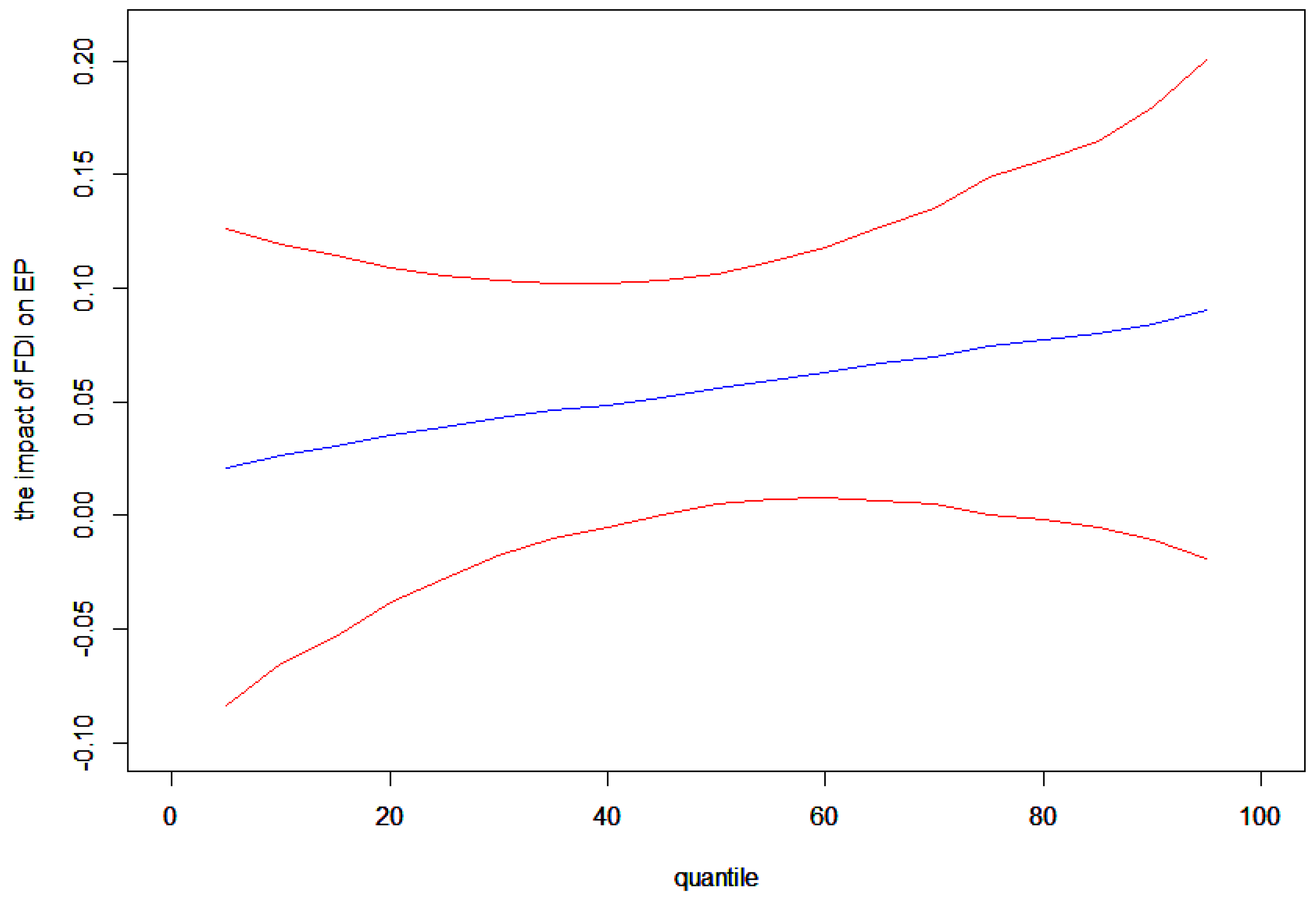
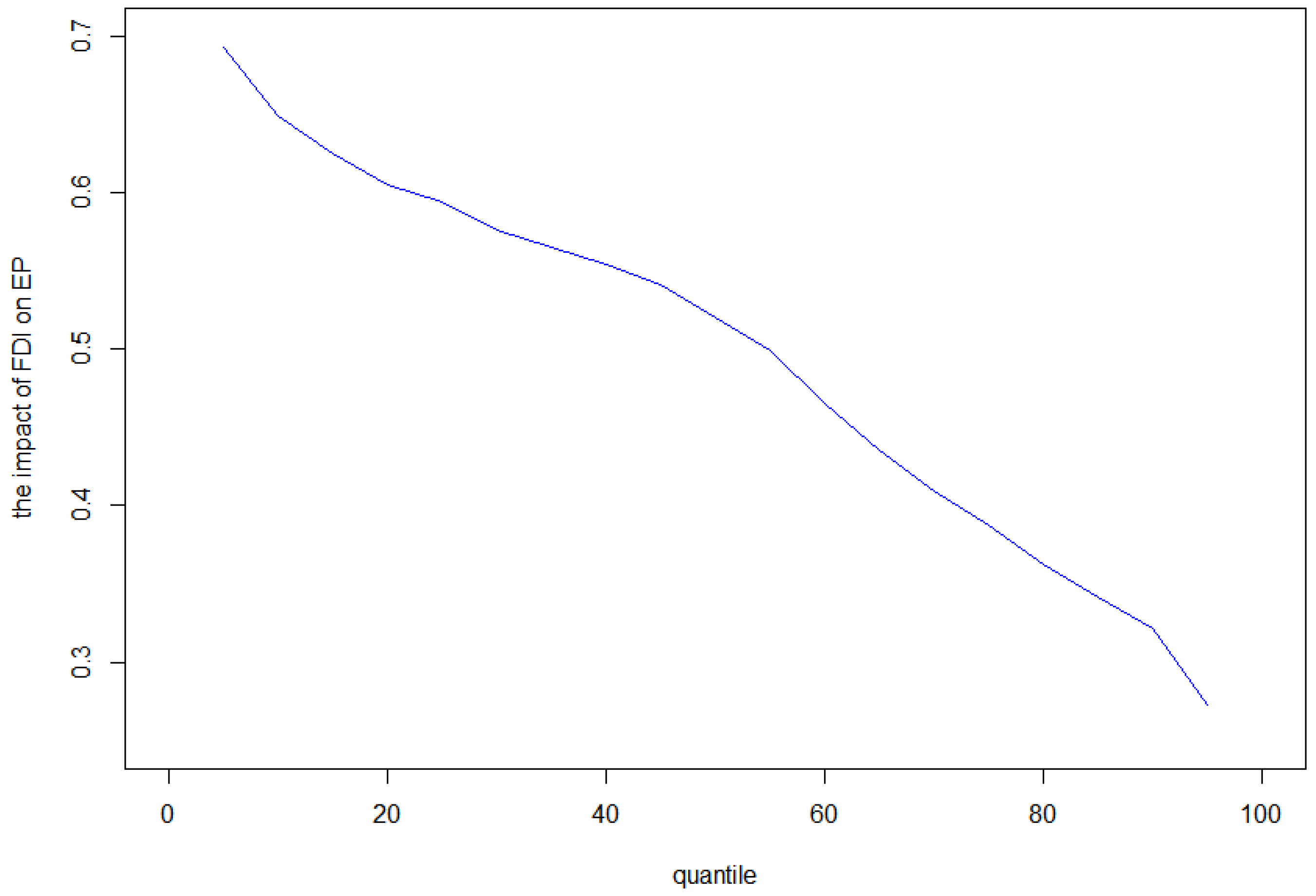
In this subsection, we use the panel quantile regression model to analyze the impact of FDI on EP at different quantile in developed countries. (Panel quantile regression results of the impact of FDI on EP in developing countries have also been computed in Table 5, but results are globally insignificant and not reported. Figure 1 presents the coefficients of FDI at different quantiles of EP in developing countries.) To be more precise about the impact of FDI on EP, we further investigate the influence of FDI on EP under different EP levels. The results in Table 6 provide detailed description throughout the conditional distribution, which are reported for the 10th–90th quantiles of the conditional distribution of EP. Additionally, the results can be divided into three separate groups, which are low quantiles (10th, 20th and 30th), middle quantiles (40th, 50th and 60th) and high quantiles (70th, 80th and 90th). The results show that there exists heterogeneity of the impact of FDI on EP at different quantiles in developed countries. Besides that, we present the coefficients and confidence intervals of FDI at different quantiles of EP in Figure 2. The results indicate that the coefficients of FDI increase with increased quantiles in developed countries.
Specifically, at the low quantiles, the impact of FDI on EP is insignificant in developed countries. The reason for the insignificant impact of FDI on EP may be that some low-EP developed countries introduce FDI, which has less effect on environmental quality and productivity. The result is somewhat consistent with the results of Kim and Baek [13], who discovered that FDI has little effect on the environment in both developed and developing countries. Therefore, FDI has an insignificant impact on EP in low-EP developed countries.
At the middle quantiles, FDI has a positive and significant influence on EP in developed countries. The coefficients of FDI at 40th, 50th and 60th quantiles are 0.048, 0.056, and 0.063 respectively. The results indicate that the impact of FDI increases gradually in middle-EP developed countries. As the quantiles of EP rise, the positive impact of FDI on EP increases, which is consistent with our expectations. We can interpret these results as evidence that middle-EP developed countries, which have better absorptive capacity than low-EP developed countries, can better use cleaner managerial and more specialized technological skills to improve their environmental quality and productivity, thus improve their EP. Therefore, in middle-EP developed countries, an increase in FDI improves the environmental quality and productivity then improves their EP.
At the high quantiles, the effect of FDI on EP is positive and significant in developed countries. The coefficients of FDI at 70th, 80th and 90th quantiles are 0.070, 0.077 and 0.084 respectively, indicating that the positive effect increases with the rise of quantile of EP. Besides that, the impact of FDI at high quantile is more positive than the impact at middle quantiles. The reason for this phenomenon is that high-EP developed countries may have achieved a desired level of productivity at the development stage, and their modes of production and techniques are more advanced. At the same time, the absorptive capacity of high-EP developed countries is higher than middle-EP developed countries, which will help them improve their EP. Therefore, the impact of FDI on EP in high-EP developed countries is more positive than middle-EP developed countries.
Overall, there are significant differences in the impact of FDI on EP across different quantiles of EP in developed countries. The different values of coefficients at different quantiles indicated that the impact of FDI varies across the conditional EP distribution in developed countries. FDI initially plays an insignificant role in EP at the low quantiles. At the middle quantiles, it becomes significantly positive, while at the high quantile, it also plays a positive and significant impact on EP. These results indicate that as the quantiles of EP increases, the positive impact of FDI on EP increases, implying that higher-EP developed countries may have better absorptive capacity to improve their EP.
5. Conclusions
The main objective of this study is to investigate the impact of FDI on EP. To achieve this objective, we first use a directional slack-based model considering undesirable output to measure the EP of 40 countries in the period 1990–2014. The sample is divided into the developed and developing countries sub-samples to explore the impact of FDI on EP. Then, we adopt the panel quantile regression model to conduct an empirical test.
Based on the empirical results, several important conclusions are drawn as follows. First, the impact of FDI on EP is not significant for the full sample. Additionally, the results indicate that there exists heterogeneity regarding the impact of FDI on EP between developed and developing countries. On the one hand, FDI has a positive and significant impact on EP in developed countries. On the other hand, FDI has an insignificant influence on EP in developing countries. Furthermore, there is heterogeneity regarding the effect of FDI on EP at different quantiles of EP in developed countries.
Accordingly, the following policy implications can be pursued to improve EP of developed and developing countries. First, each country should set strict environmental standards to introduce FDI scientifically. Because the enforcement of stringent environmental laws can ensure environmental quality [39]. Host countries should attempt to assess the impact of FDI on EP before introducing foreign investors. Developing countries should try to set stricter environmental policies and entry standards of FDI to strengthen their productivity and improve their environmental quality, rather than introducing FDI at the cost of environment, and this will be beneficial to improve their EP. For developed countries, they can further optimize their FDI activities through their better absorptive capacity to improve their EP.
Second, panel quantile regression results provide the scientific basis for policymakers to target policies to a specific country with different levels of EP rather than to the entire group. Low-EP developed countries should set stricter environmental policies and entry standards of FDI to improve the quality of FDI and enhance their productivity, thus improving their EP. In middle-EP developed countries, their environmental policies and entry standards of FDI are more effective, so they can improve their absorptive capacity to further improve their productivity and EP. As for high-EP developed countries, they should optimize their FDI activity to improve their EP.
To conclude, the most important implication of our findings is that uniform entry policies of FDI are unlikely to succeed equally across 40 countries with different productivity levels. Therefore, the entry policies of FDI should be tailored differently across developing countries, low-EP, middle-EP and high-EP developed countries, thus can effectively absorb more FDI to improve their productivity and their EP at the same time.
Author Contributions
Conceptualization, Z.L., H.D., Z.H. and P.F.; Data curation, H.D. and Z.H.; Formal analysis, Z.L., H.D., Z.H. and P.F.; Funding acquisition, Z.L.; Investigation, Z.L. and P.F.; Methodology, H.D. and Z.H.; Resources, Z.L. and P.F.; Software, H.D. and Z.H.; Supervision, Z.L. and P.F.; Validation Z.L., H.D., Z.H. and P.F.; Writing—original draft, Z.L., H.D., Z.H. and P.F.; Writing—review & editing, Z.L., H.D., Z.H. and P.F.
Funding
This research was funded by the Humanities and Social sciences fund of department of education of Guangdong Province, grant number 2016WZDXM023.
Acknowledgments
Authors would like to thank Guangzhou University for sponsoring this research.
Conflicts of Interest
The authors declare no conflicts of interest.
Appendix A

Table A1.
Environmental performance of developed countries.
| Year | AUS | AUT | CAN | CHE | CYP | CZE | DEU | DNK | ESP | FIN | FRA | GBR |
| 1990 | 0.643 | 0.634 | 0.595 | 0.816 | 0.473 | 0.434 | 0.577 | 0.755 | 0.608 | 0.540 | 0.649 | 0.613 |
| 1991 | 0.638 | 0.634 | 0.586 | 0.803 | 0.472 | 0.393 | 0.594 | 0.726 | 0.610 | 0.524 | 0.645 | 0.605 |
| 1992 | 0.633 | 0.648 | 0.583 | 0.803 | 0.492 | 0.390 | 0.604 | 0.751 | 0.610 | 0.534 | 0.657 | 0.608 |
| 1993 | 0.636 | 0.647 | 0.586 | 0.813 | 0.487 | 0.392 | 0.603 | 0.741 | 0.614 | 0.530 | 0.655 | 0.616 |
| 1994 | 0.643 | 0.653 | 0.593 | 0.817 | 0.501 | 0.403 | 0.611 | 0.751 | 0.616 | 0.529 | 0.670 | 0.627 |
| 1995 | 0.646 | 0.655 | 0.596 | 0.827 | 0.529 | 0.420 | 0.615 | 0.770 | 0.618 | 0.550 | 0.672 | 0.635 |
| 1996 | 0.644 | 0.653 | 0.595 | 0.824 | 0.524 | 0.424 | 0.611 | 0.738 | 0.628 | 0.544 | 0.667 | 0.635 |
| 1997 | 0.649 | 0.659 | 0.600 | 0.828 | 0.534 | 0.413 | 0.620 | 0.775 | 0.628 | 0.559 | 0.682 | 0.653 |
| 1998 | 0.654 | 0.667 | 0.606 | 0.839 | 0.546 | 0.411 | 0.626 | 0.785 | 0.631 | 0.578 | 0.686 | 0.661 |
| 1999 | 0.661 | 0.679 | 0.614 | 0.849 | 0.558 | 0.423 | 0.636 | 0.812 | 0.632 | 0.592 | 0.699 | 0.670 |
| 2000 | 0.664 | 0.688 | 0.621 | 0.877 | 0.568 | 0.425 | 0.642 | 0.847 | 0.636 | 0.614 | 0.712 | 0.678 |
| 2001 | 0.667 | 0.681 | 0.623 | 0.857 | 0.583 | 0.429 | 0.642 | 0.829 | 0.641 | 0.610 | 0.709 | 0.685 |
| 2002 | 0.668 | 0.684 | 0.627 | 0.867 | 0.590 | 0.430 | 0.647 | 0.830 | 0.638 | 0.603 | 0.711 | 0.698 |
| 2003 | 0.670 | 0.674 | 0.619 | 0.867 | 0.581 | 0.435 | 0.646 | 0.811 | 0.639 | 0.596 | 0.709 | 0.705 |
| 2004 | 0.673 | 0.681 | 0.621 | 0.880 | 0.606 | 0.451 | 0.650 | 0.840 | 0.634 | 0.609 | 0.716 | 0.713 |
| 2005 | 0.673 | 0.682 | 0.624 | 0.892 | 0.619 | 0.468 | 0.655 | 0.862 | 0.634 | 0.642 | 0.719 | 0.721 |
| 2006 | 0.665 | 0.694 | 0.627 | 0.906 | 0.624 | 0.485 | 0.663 | 0.842 | 0.641 | 0.628 | 0.729 | 0.731 |
| 2007 | 0.664 | 0.709 | 0.624 | 0.958 | 0.628 | 0.497 | 0.684 | 0.854 | 0.643 | 0.647 | 0.738 | 0.745 |
| 2008 | 0.661 | 0.711 | 0.618 | 0.944 | 0.626 | 0.503 | 0.685 | 0.856 | 0.649 | 0.662 | 0.734 | 0.743 |
| 2009 | 0.657 | 0.703 | 0.611 | 0.911 | 0.623 | 0.494 | 0.669 | 0.835 | 0.652 | 0.641 | 0.723 | 0.742 |
| 2010 | 0.656 | 0.697 | 0.615 | 0.950 | 0.635 | 0.491 | 0.677 | 0.832 | 0.656 | 0.627 | 0.728 | 0.739 |
| 2011 | 0.656 | 0.711 | 0.618 | 0.966 | 0.639 | 0.501 | 0.697 | 0.871 | 0.656 | 0.647 | 0.745 | 0.765 |
| 2012 | 0.665 | 0.715 | 0.622 | 0.961 | 0.644 | 0.499 | 0.694 | 0.893 | 0.650 | 0.658 | 0.741 | 0.760 |
| 2013 | 0.671 | 0.710 | 0.625 | 0.948 | 0.650 | 0.497 | 0.690 | 0.884 | 0.661 | 0.659 | 0.741 | 0.772 |
| 2014 | 0.678 | 0.720 | 0.625 | 1.000 | 0.645 | 0.506 | 0.703 | 1.000 | 0.669 | 0.655 | 0.758 | 0.806 |
| 1990 | 0.554 | 0.643 | 0.744 | 0.633 | 0.570 | 0.352 | 0.619 | 0.899 | 0.756 | 0.571 | 0.629 | 0.584 |
| Year | GRC | IRL | ISR | ITA | JPN | KOR | NLD | NOR | NZL | PRT | SWE | USA |
| 1991 | 0.566 | 0.644 | 0.748 | 0.635 | 0.578 | 0.376 | 0.616 | 0.905 | 0.695 | 0.580 | 0.624 | 0.580 |
| 1992 | 0.567 | 0.654 | 0.726 | 0.640 | 0.577 | 0.375 | 0.622 | 0.923 | 0.677 | 0.573 | 0.627 | 0.586 |
| 1993 | 0.563 | 0.657 | 0.678 | 0.643 | 0.576 | 0.374 | 0.623 | 0.906 | 0.716 | 0.570 | 0.624 | 0.588 |
| 1994 | 0.565 | 0.664 | 0.667 | 0.657 | 0.572 | 0.389 | 0.631 | 0.945 | 0.730 | 0.570 | 0.633 | 0.594 |
| 1995 | 0.571 | 0.692 | 0.655 | 0.659 | 0.579 | 0.399 | 0.626 | 0.967 | 0.725 | 0.572 | 0.646 | 0.596 |
| 1996 | 0.576 | 0.703 | 0.654 | 0.665 | 0.586 | 0.403 | 0.627 | 1.000 | 0.696 | 0.583 | 0.650 | 0.601 |
| 1997 | 0.584 | 0.724 | 0.645 | 0.671 | 0.588 | 0.402 | 0.644 | 1.000 | 0.662 | 0.588 | 0.669 | 0.606 |
| 1998 | 0.584 | 0.731 | 0.646 | 0.673 | 0.590 | 0.391 | 0.656 | 0.978 | 0.649 | 0.589 | 0.682 | 0.612 |
| 1999 | 0.593 | 0.782 | 0.654 | 0.677 | 0.588 | 0.418 | 0.674 | 0.954 | 0.649 | 0.585 | 0.703 | 0.617 |
| 2000 | 0.595 | 0.831 | 0.661 | 0.687 | 0.596 | 0.429 | 0.685 | 0.976 | 0.646 | 0.594 | 0.729 | 0.619 |
| 2001 | 0.602 | 0.799 | 0.645 | 0.691 | 0.600 | 0.437 | 0.684 | 0.965 | 0.649 | 0.594 | 0.722 | 0.618 |
| 2002 | 0.611 | 0.800 | 0.646 | 0.686 | 0.601 | 0.453 | 0.677 | 1.000 | 0.663 | 0.587 | 0.714 | 0.618 |
| 2003 | 0.623 | 0.796 | 0.636 | 0.677 | 0.607 | 0.455 | 0.672 | 0.951 | 0.668 | 0.588 | 0.731 | 0.621 |
| 2004 | 0.633 | 0.808 | 0.656 | 0.680 | 0.611 | 0.461 | 0.676 | 1.000 | 0.665 | 0.589 | 0.749 | 0.626 |
| 2005 | 0.630 | 0.817 | 0.674 | 0.680 | 0.618 | 0.472 | 0.685 | 1.000 | 0.669 | 0.586 | 0.769 | 0.630 |
| 2006 | 0.647 | 0.829 | 0.671 | 0.686 | 0.624 | 0.483 | 0.698 | 0.990 | 0.671 | 0.597 | 0.797 | 0.634 |
| 2007 | 0.653 | 0.837 | 0.682 | 0.691 | 0.629 | 0.490 | 0.710 | 0.989 | 0.676 | 0.603 | 0.813 | 0.632 |
| 2008 | 0.649 | 0.807 | 0.669 | 0.687 | 0.632 | 0.490 | 0.713 | 0.909 | 0.659 | 0.608 | 0.797 | 0.632 |
| 2009 | 0.638 | 0.797 | 0.680 | 0.678 | 0.624 | 0.486 | 0.698 | 0.898 | 0.667 | 0.600 | 0.787 | 0.631 |
| 2010 | 0.630 | 0.810 | 0.679 | 0.683 | 0.633 | 0.489 | 0.691 | 0.873 | 0.665 | 0.617 | 0.781 | 0.636 |
| 2011 | 0.607 | 0.857 | 0.689 | 0.690 | 0.639 | 0.491 | 0.708 | 0.957 | 0.672 | 0.615 | 0.791 | 0.641 |
| 2012 | 0.592 | 0.854 | 0.674 | 0.688 | 0.645 | 0.493 | 0.703 | 0.937 | 0.664 | 0.612 | 0.797 | 0.649 |
| 2013 | 0.603 | 0.863 | 0.699 | 0.693 | 0.651 | 0.497 | 0.701 | 0.891 | 0.668 | 0.614 | 0.808 | 0.651 |
| 2014 | 0.612 | 1.000 | 0.712 | 0.706 | 0.657 | 0.502 | 0.715 | 1.000 | 0.666 | 0.620 | 0.826 | 0.654 |
Table A2.
Environmental performance of developing countries.
| Year | ARG | BRA | CHL | CHN | EGY | IDN | IND | IRN | MEX | MYS | PHL | POL | RUS | THA | TUR | ZAF |
|---|---|---|---|---|---|---|---|---|---|---|---|---|---|---|---|---|
| 1990 | 0.974 | 0.799 | 0.919 | 1.000 | 0.456 | 0.429 | 0.408 | 0.558 | 0.599 | 0.473 | 0.486 | 0.606 | −0.721 | 0.139 | 0.767 | 0.593 |
| 1991 | 1.000 | 0.761 | 0.966 | 1.000 | 0.453 | 0.424 | 0.382 | 0.575 | 0.596 | 0.466 | 0.476 | 0.575 | −0.775 | 0.169 | 0.730 | 0.570 |
| 1992 | 0.879 | 0.717 | 1.000 | 0.965 | 0.460 | 0.424 | 0.378 | 0.555 | 0.589 | 0.466 | 0.462 | 0.577 | −1.040 | 0.193 | 0.730 | 0.556 |
| 1993 | 1.000 | 0.728 | 1.000 | 0.865 | 0.461 | 0.424 | 0.378 | 0.533 | 0.578 | 0.464 | 0.461 | 0.581 | −1.137 | 0.213 | 0.741 | 0.547 |
| 1994 | 0.930 | 0.735 | 0.966 | 0.749 | 0.473 | 0.435 | 0.382 | 0.502 | 0.584 | 0.469 | 0.458 | 0.596 | −1.312 | 0.225 | 0.655 | 0.548 |
| 1995 | 0.845 | 0.727 | 1.000 | 0.597 | 0.476 | 0.440 | 0.387 | 0.501 | 0.551 | 0.461 | 0.456 | 0.606 | −1.300 | 0.232 | 0.667 | 0.545 |
| 1996 | 0.840 | 0.689 | 1.000 | 0.508 | 0.480 | 0.439 | 0.392 | 0.510 | 0.563 | 0.460 | 0.462 | 0.607 | −1.282 | 0.225 | 0.670 | 0.549 |
| 1997 | 0.853 | 0.669 | 1.000 | 0.500 | 0.484 | 0.429 | 0.383 | 0.495 | 0.579 | 0.452 | 0.457 | 0.609 | −1.134 | 0.191 | 0.678 | 0.543 |
| 1998 | 0.834 | 0.651 | 0.886 | 0.493 | 0.483 | 0.386 | 0.390 | 0.487 | 0.586 | 0.425 | 0.448 | 0.606 | −1.150 | 0.161 | 0.649 | 0.531 |
| 1999 | 0.767 | 0.641 | 0.835 | 0.488 | 0.487 | 0.372 | 0.401 | 0.471 | 0.575 | 0.443 | 0.450 | 0.601 | −0.948 | 0.188 | 0.591 | 0.531 |
| 2000 | 0.740 | 0.648 | 0.851 | 0.486 | 0.496 | 0.376 | 0.397 | 0.478 | 0.580 | 0.448 | 0.453 | 0.599 | −0.705 | 0.218 | 0.597 | 0.538 |
| 2001 | 0.701 | 0.643 | 0.865 | 0.485 | 0.498 | 0.374 | 0.400 | 0.462 | 0.563 | 0.437 | 0.460 | 0.581 | −0.563 | 0.236 | 0.582 | 0.541 |
| 2002 | 0.624 | 0.649 | 0.847 | 0.477 | 0.494 | 0.380 | 0.398 | 0.466 | 0.556 | 0.446 | 0.465 | 0.575 | −0.441 | 0.261 | 0.590 | 0.546 |
| 2003 | 0.665 | 0.652 | 0.842 | 0.456 | 0.493 | 0.391 | 0.413 | 0.473 | 0.548 | 0.447 | 0.473 | 0.574 | −0.307 | 0.289 | 0.594 | 0.541 |
| 2004 | 0.684 | 0.657 | 0.848 | 0.439 | 0.496 | 0.393 | 0.420 | 0.466 | 0.551 | 0.457 | 0.486 | 0.584 | −0.188 | 0.307 | 0.609 | 0.539 |
| 2005 | 0.718 | 0.659 | 0.835 | 0.435 | 0.493 | 0.403 | 0.435 | 0.457 | 0.544 | 0.461 | 0.494 | 0.580 | −0.094 | 0.318 | 0.618 | 0.545 |
| 2006 | 0.731 | 0.666 | 0.830 | 0.443 | 0.500 | 0.412 | 0.441 | 0.456 | 0.546 | 0.471 | 0.510 | 0.583 | −0.001 | 0.333 | 0.612 | 0.545 |
| 2007 | 0.761 | 0.673 | 0.798 | 0.453 | 0.501 | 0.419 | 0.440 | 0.463 | 0.546 | 0.473 | 0.518 | 0.590 | 0.084 | 0.349 | 0.603 | 0.542 |
| 2008 | 0.738 | 0.672 | 0.759 | 0.445 | 0.502 | 0.421 | 0.424 | 0.446 | 0.541 | 0.474 | 0.516 | 0.573 | 0.132 | 0.349 | 0.595 | 0.521 |
| 2009 | 0.673 | 0.676 | 0.698 | 0.431 | 0.501 | 0.416 | 0.420 | 0.435 | 0.524 | 0.465 | 0.518 | 0.560 | 0.095 | 0.340 | 0.576 | 0.490 |
| 2010 | 0.711 | 0.669 | 0.682 | 0.420 | 0.505 | 0.426 | 0.426 | 0.438 | 0.535 | 0.472 | 0.523 | 0.547 | 0.132 | 0.360 | 0.580 | 0.492 |
| 2011 | 0.714 | 0.668 | 0.656 | 0.408 | 0.493 | 0.417 | 0.418 | 0.431 | 0.534 | 0.477 | 0.527 | 0.551 | 0.169 | 0.358 | 0.592 | 0.490 |
| 2012 | 0.670 | 0.655 | 0.624 | 0.397 | 0.488 | 0.419 | 0.408 | 0.392 | 0.534 | 0.481 | 0.531 | 0.552 | 0.194 | 0.374 | 0.592 | 0.488 |
| 2013 | 0.657 | 0.647 | 0.607 | 0.387 | 0.490 | 0.440 | 0.407 | 0.384 | 0.534 | 0.474 | 0.536 | 0.549 | 0.214 | 0.374 | 0.609 | 0.485 |
| 2014 | 0.600 | 0.633 | 0.608 | 0.380 | 0.494 | 0.448 | 0.406 | 0.389 | 0.541 | 0.478 | 0.536 | 0.556 | 0.227 | 0.370 | 0.607 | 0.477 |
References
- Asghari, M. Does FDI promote MENA region’s environment quality? Pollution halo or pollution haven hypothesis. Int. J. Sci. Res. Environ. Sci. 2013, 1, 92–100. [Google Scholar] [CrossRef]
- Pao, H.T.; Tsai, C.M. Multivariate Granger causality between CO2 emissions, energy consumption, FDI (foreign direct investment) and GDP (gross domestic product): evidence from a panel of BRIC (Brazil, Russian Federation, India, and China) countries. Energy 2011, 36, 685–693. [Google Scholar] [CrossRef]
- Sapkota, P.; Bastola, U. Foreign direct investment, income, and environmental pollution in developing countries: Panel data analysis of Latin America. Energy Econ. 2017, 64, 206–212. [Google Scholar] [CrossRef]
- Shahbaz, M.; Nasreen, S.; Abbas, F.; Anis, O. Does foreign direct investment impede environmental quality in high-, middle-, and low-income countries? Energy Econ. 2015, 51, 275–287. [Google Scholar] [CrossRef]
- Cole, M.A.; Elliott, R.J.; Strobl, E. The environmental performance of firms: The role of foreign ownership, training, and experience. Ecol. Econ. 2008, 65, 538–546. [Google Scholar] [CrossRef]
- Abdouli, M.; Hammami, S. The dynamic links between environmental quality, foreign direct investment, and economic growth in the Middle Eastern and North African countries (MENA region). J. Knowl. Econ. 2018, 9, 833–853. [Google Scholar] [CrossRef]
- Al-Mulali, U.; Tang, C.F. Investigating the validity of pollution haven hypothesis in the gulf cooperation council (GCC) countries. Energy Policy 2013, 60, 813–819. [Google Scholar] [CrossRef]
- Chandran, V.G.R.; Tang, C.F. The impacts of transport energy consumption, foreign direct investment and income on CO2 emissions in ASEAN-5 economies. Renew. Sustain. Energy Rev. 2013, 24, 445–453. [Google Scholar] [CrossRef]
- Seker, F.; Ertugrul, H.M.; Cetin, M. The impact of foreign direct investment on environmental quality: A bounds testing and causality analysis for Turkey. Renew. Sustain. Energy Rev. 2015, 52, 347–356. [Google Scholar] [CrossRef]
- Baek, J. A new look at the FDI–income–energy–environment nexus: dynamic panel data analysis of ASEAN. Energy Policy 2016, 91, 22–27. [Google Scholar] [CrossRef]
- Zugravu-Soilita, N. How does foreign direct investment affect pollution? Toward a better understanding of the direct and conditional effects. Environ. Resour. Econ. 2017, 66, 293–338. [Google Scholar] [CrossRef]
- Zarsky, L. Havens, halos and spaghetti: untangling the evidence about foreign direct investment and the environment. Foreign Direct Invest. Environ. 1999, 13, 47–74. [Google Scholar]
- Kim, H.S.; Baek, J. The environmental consequences of economic growth revisited. Econ. Bull. 2011, 31, 1198–1211. [Google Scholar]
- Hu, J.; Wang, Z.; Lian, Y.; Huang, Q. Environmental regulation, foreign direct investment and green technological progress—Evidence from Chinese manufacturing industries. Int. J. Environ. Res. Public Health 2018, 15, 221. [Google Scholar] [CrossRef]
- Zhang, J.; Fang, H.; Peng, B.; Wang, X.; Fang, S. Productivity growth-accounting for undesirable outputs and its influencing factors: The case of China. Sustainability 2016, 8, 1166. [Google Scholar] [CrossRef]
- Yu, G.; Xu, S. Industrial Agglomeration, Foreign Direct Investment and Green Total Factor Productivity―Evidence from Manufacturing Industries in Chongqing, China. Preprints 2018. [Google Scholar] [CrossRef]
- Hettige, H.; Huq, M.; Pargal, S.; Wheeler, D. Determinants of pollution abatement in developing countries: Evidence from South and Southeast Asia. World Dev. 1996, 24, 1891–1904. [Google Scholar] [CrossRef]
- Li, Z.; Huang, Z.; Dong, H. The Influential Factors on Outward Foreign Direct Investment: Evidence from the “The Belt and Road”. Emerg. Mark. Financ. Trade 2019, 1–16. [Google Scholar] [CrossRef]
- Omri, A. The nexus among foreign investment, domestic capital and economic growth: Empirical evidence from the MENA region. Res. Econ. 2014, 68, 257–263. [Google Scholar] [CrossRef] [Green Version]
- Song, M.L.; Fisher, R.; Wang, J.L.; Cui, L.B. Environmental performance evaluation with big data: Theories and methods. Ann. Oper. Res. 2018, 270, 459–472. [Google Scholar] [CrossRef]
- Galdeano-Gómez, E.; Céspedes-Lorente, J.; Martinez-del-Rio, J. Environmental performance and spillover effects on productivity: Evidence from horticultural firms. J. Environ. Manag. 2008, 88, 1552–1561. [Google Scholar] [CrossRef]
- Zhong, J.; Wang, M.; Drakeford, B.; Li, T. Spillover effects between oil and natural gas prices: Evidence from emerging and developed markets. Green Financ. 2019, 1, 30–45. [Google Scholar] [CrossRef]
- Broni, M.Y.; Hosen, M.; Masih, M. Does a country’s external debt level affect its Islamic banking sector development? evidence from Malaysia based on quantile regression and markov regime switching. Quant. Financ. Econ. 2019, 3, 366–389. [Google Scholar] [CrossRef]
- Girma, S.; Görg, H. Foreign Direct Investment, Spillovers and Absorptive Capacity: Evidence From Quantile Regressions; Deutsche Bundesbank: Frankfurt, Germany, 2005. [Google Scholar]
- Canay, I.A. A simple approach to quantile regression for panel data. Econom. J. 2011, 14, 368–386. [Google Scholar] [CrossRef]
- Qamruzzaman, M.; Wei, J. Do financial inclusion, stock market development attract foreign capital flows in developing economy: A panel data investigation. Quant. Financ. Econ. 2019, 3, 88–108. [Google Scholar] [CrossRef]
- Li, Z.; Dong, H.; Huang, Z.; Failler, P. Asymmetric effects on risks of Virtual Financial Assets (VFAs) in different regimes: A Case of Bitcoin. Quant. Financ. Econ. 2018, 2, 860–883. [Google Scholar] [CrossRef]
- Machado, J.A.; Silva, J.S. Quantiles via moments. J. Econ. 2019. [Google Scholar] [CrossRef]
- Picazo-Tadeo, A.J.; Castillo-Giménez, J.; Beltrán-Esteve, M. An intertemporal approach to measuring environmental performance with directional distance functions: Greenhouse gas emissions in the European Union. Ecol. Econ. 2014, 100, 173–182. [Google Scholar] [CrossRef]
- Kortelainen, M. Dynamic environmental performance analysis: A Malmquist index approach. Ecol. Econ. 2008, 64, 701–715. [Google Scholar] [CrossRef]
- Oh, D.H. A global Malmquist-Luenberger productivity index. J. Prod. Anal. 2010, 34, 183–197. [Google Scholar] [CrossRef]
- Fukuyama, H.; Weber, W.L. A directional slacks-based measure of technical inefficiency. Socio-Econ. Plan. Sci. 2009, 43, 274–287. [Google Scholar] [CrossRef]
- Liu, Z.; Xin, L. Has China’s Belt and Road Initiative promoted its green total factor productivity?— Evidence from primary provinces along the route. Energy Policy 2019, 129, 360–369. [Google Scholar] [CrossRef]
- Hall, R.E.; Jones, C.I. Why do some countries produce so much more output per worker than others? Q. J. Econ. 1999, 114, 83–116. [Google Scholar] [CrossRef]
- Emrouznejad, A.; Yang, G.L. A framework for measuring global Malmquist–Luenberger productivity index with CO2 emissions on Chinese manufacturing industries. Energy 2016, 115, 840–856. [Google Scholar] [CrossRef]
- Liao, G.; Drakeford, B. An analysis of financial support, technological progress and energy efficiency: Evidence from China. Green Financ. 2019, 1, 174–187. [Google Scholar] [CrossRef]
- Li, Z.; Liao, G.; Wang, Z.; Huang, Z. Green loan and subsidy for promoting clean production innovation. J. Clean Prod. 2018, 187, 421–431. [Google Scholar] [CrossRef]
- Huang, Z.; Liao, G.; Li, Z. Loaning scale and government subsidy for promoting green innovation. Technol. Forecast. Soc. Chang. 2019, 144, 148–156. [Google Scholar] [CrossRef]
- Kwakwa, P.W.; Alhassan, H.; Aboagye, S. Environmental Kuznets curve hypothesis in a financial development and natural resource extraction context: Evidence from Tunisia. Quant. Financ. Econ. 2018, 2, 981–1000. [Google Scholar] [CrossRef]
Figure 1.
Panel quantile regression results of developing countries. Notes: The blue line represents the coefficient of FDI at different quantiles of EP in developing countries.
Figure 1.
Panel quantile regression results of developing countries. Notes: The blue line represents the coefficient of FDI at different quantiles of EP in developing countries.

Figure 2.
Panel quantile regression results of developed countries. Notes: The blue line represents the coefficient of FDI at different quantiles of EP in developed countries. The top red line represents the upper confidence limits, while the bottom red line represents the lower confidence limits.
Figure 2.
Panel quantile regression results of developed countries. Notes: The blue line represents the coefficient of FDI at different quantiles of EP in developed countries. The top red line represents the upper confidence limits, while the bottom red line represents the lower confidence limits.

Table 1.
Explanatory and control variables.
| Variable | Abbreviation | Measurement | Source | |
|---|---|---|---|---|
| Explanatory Variable | Foreign direct investment | FDI | net inflows of FDI/GDP | World Bank |
| Control Variable | Innovation capacity | LnInno | Log (Patent applications per million people) | World Intellectual Property Organization Statistics Database |
| Industrial structure | Indus | output value of the secondary industry/GDP | EPS macro database | |
| Energy structure | Ener | Renewable energy consumption/total final energy consumption | EPS macro database |
Table 2.
Descriptive statistics and results of T test.
| Variable | Sample | Mean | Std.Dev. | Min | 0.25 | 0.5 | 0.75 | Max | T Value |
|---|---|---|---|---|---|---|---|---|---|
| EP | 1 | 59.049 | 24.170 | −131.24 | 49.753 | 61.981 | 68.220 | 100 | — |
| 2 | 66.483 | 11.963 | 35.171 | 60.842 | 64.956 | 70.882 | 100 | −11.031 | |
| 3 | 47.898 | 32.250 | −131.24 | 42.886 | 49.583 | 60.045 | 100 | ||
| FDI | 1 | 3.253 | 8.345 | −43.463 | 0.842 | 1.952 | 3.568 | 198.074 | — |
| 2 | 3.841 | 10.604 | −43.463 | 0.824 | 1.923 | 3.792 | 198.074 | −3.303 | |
| 3 | 2.371 | 2.061 | −2.757 | 0.897 | 2.021 | 3.273 | 11.654 | ||
| LnInno | 1 | 5.203 | 1.483 | 0.964 | 4.257 | 5.200 | 6.248 | 8.329 | — |
| 2 | 5.901 | 1.290 | 0.964 | 5.139 | 5.898 | 6.866 | 8.330 | −23.095 | |
| 3 | 4.156 | 1.083 | 1.330 | 3.307 | 4.496 | 5.016 | 6.523 | ||
| Indus | 1 | 31.152 | 6.761 | 10.7 | 26.325 | 30.5 | 36.15 | 50.1 | — |
| 2 | 28.210 | 5.581 | 10.7 | 24.4 | 27.6 | 31.3 | 44.8 | 19.672 | |
| 3 | 35.564 | 5.928 | 23.8 | 31.5 | 34.7 | 39.55 | 50.1 | ||
| Ener | 1 | 17.269 | 15.273 | 0.335 | 5.433 | 10.736 | 26.830 | 61.379 | — |
| 2 | 14.688 | 14.181 | 0.335 | 4.535 | 8.594 | 22.618 | 61.379 | 6.527 | |
| 3 | 21.142 | 16.034 | 0.438 | 7.577 | 16.881 | 32.866 | 58.653 |
Notes: (1) “Ln” means the variable in natural logarithms; (2) To express EP more clearly, this study multiplied it by 100. (3) Sample 1, 2, 3 represent full sample, developed countries sample, developing countries sample, respectively.
Table 3.
Fixed, random effect and panel quantile regression estimation for the full sample.
| Variable | Fixed Effect Model | Random Effect Model | Panel Quantile Regression | ||||
|---|---|---|---|---|---|---|---|
| 10th | 25th | 50th | 75th | 90th | |||
| FDI | 0.059 | 0.060 | 0.025 | 0.039 | 0.055 | 0.079 | 0.091 |
| (0.042) | (0.042) | (0.179) | (0.136) | (0.087) | (0.052) | (0.073) | |
| LnInno | −1.279 * | −0.834 | 0.035 | −0.494 | −1.137 | −2.093 ** | −2.575 ** |
| (0.688) | (0.656) | (3.074) | (2.336) | (1.498) | (0.884) | (1.244) | |
| Indus | −0.772 *** | −0.819 *** | −0.943 | −0.874 | −0.791 | −0.666 ** | −0.603 |
| (0.120) | (0.115) | (1.126) | (0.856) | (0.548) | (0.323) | (0.456) | |
| Ener | 0.339 *** | 0.344 *** | 0.144 | 0.222 | 0.318 | 0.459 *** | 0.531 *** |
| (0.107) | (0.096) | (0.430) | (0.327) | (0.210) | (0.124) | (0.174) | |
| cons | 83.71 *** | 82.76 *** | |||||
| (6.016) | (6.406) | ||||||
Notes: (1) Standard errors are in parentheses. (2) ***, **, and * indicate significance at the 1%, 5%, and 10% levels, respectively.
Table 4.
Fixed and random effects estimation for developed and developing countries.
| Variable | Developed Countries | Developing Countries | ||
|---|---|---|---|---|
| Fixed Effect Model | Random Effect Model | Fixed Effect Model | Random Effect Model | |
| FDI | 0.0557 *** | 0.0559 *** | 0.492 | 0.584 |
| (0.013) | (0.013) | (0.537) | (0.533) | |
| LnInno | −1.630 *** | −1.581 *** | −1.435 | −1.395 |
| (0.305) | (0.301) | (1.554) | (1.513) | |
| Indus | −0.314 *** | −0.333 *** | −0.978 *** | −0.977 *** |
| (0.060) | (0.058) | (0.245) | (0.241) | |
| Ener | 0.692 *** | 0.668 *** | 0.172 | 0.204 |
| (0.050) | (0.047) | (0.237) | (0.212) | |
| _cons | 74.57 *** | 75.19 *** | 83.82 *** | 82.76 *** |
| (2.812) | (3.374) | (12.76) | (13.88) | |
| N | 600 | 600 | 400 | 400 |
Notes: (1) Standard errors are in parentheses. (2) ***, **, and * indicate significance at the 1%, 5%, and 10% levels, respectively.
Table 5.
Panel quantile regression results of developing countries.
| Variable | 10th | 20th | 30th | 40th | 50th | 60th | 70th | 80th | 90th |
|---|---|---|---|---|---|---|---|---|---|
| FDI | 0.649 | 0.605 | 0.576 | 0.554 | 0.520 | 0.465 | 0.409 | 0.362 | 0.322 |
| (9.987) | (8.429) | (7.398) | (6.626) | (5.421) | (3.478) | (1.643) | (0.901) | (1.896) | |
| LnInno | 1.047 | 0.353 | −0.108 | −0.453 | −0.993 | −1.872 | −2.745 | −3.501 | −4.121 |
| (23.74) | (20.04) | (17.59) | (15.76) | (12.89) | (8.273) | (3.912) | (2.146) | (4.512) | |
| Indus | −1.217 | −1.150 | −1.105 | −1.072 | −1.020 | −0.935 | −0.851 | −0.778 | −0.719 |
| (7.329) | (6.185) | (5.429) | (4.862) | (3.978) | (2.552) | (1.206) | (0.661) | (1.392) | |
| Ener | 0.047 | 0.082 | 0.105 | 0.123 | 0.150 | 0.194 | 0.238 | 0.276 | 0.307 |
| (2.446) | (2.065) | (1.812) | (1.623) | (1.328) | (0.852) | (0.402) | (0.221) | (0.464) | |
| N | 400 | 400 | 400 | 400 | 400 | 400 | 400 | 400 | 400 |
Notes: (1) Standard errors are in parentheses. (2) ***, **, and * indicate significance at the 1%, 5%, and 10% levels, respectively.
Table 6.
Panel quantile regression results of developed countries.
| Variable | 10th | 20th | 30th | 40th | 50th | 60th | 70th | 80th | 90th |
|---|---|---|---|---|---|---|---|---|---|
| FDI | 0.027 | 0.035 | 0.043 | 0.048 * | 0.056 ** | 0.063 ** | 0.070 ** | 0.077 * | 0.084 * |
| (0.047) | (0.038) | (0.031) | (0.028) | (0.026) | (0.028) | (0.033) | (0.040) | (0.049) | |
| LnInno | −1.472 ** | −1.520 *** | −1.560 *** | −1.589 *** | −1.630 *** | −1.668 *** | −1.707 *** | −1.746 *** | −1.786 *** |
| (0.654) | (0.521) | (0.428) | (0.381) | (0.358) | (0.388) | (0.461) | (0.561) | (0.675) | |
| Indus | −0.473 *** | −0.425 *** | −0.385 *** | −0.355 *** | −0.314 *** | −0.276 *** | −0.236 *** | −0.196 * | −0.156 |
| (0.125) | (0.100) | (0.082) | (0.074) | (0.069) | (0.075) | (0.089) | (0.108) | (0.129) | |
| Ener | 0.581 *** | 0.615 *** | 0.643 *** | 0.664 *** | 0.692 *** | 0.719 *** | 0.747 *** | 0.775 *** | 0.802 *** |
| (0.087) | (0.070) | (0.057) | (0.051) | (0.048) | (0.052) | (0.062) | (0.075) | (0.090) | |
| N | 600 | 600 | 600 | 600 | 600 | 600 | 600 | 600 | 600 |
Notes: (1) Standard errors are in parentheses. (2) ***, **, and * indicate significance at the 1%, 5%, and 10% levels, respectively.
© 2019 by the authors. Licensee MDPI, Basel, Switzerland. This article is an open access article distributed under the terms and conditions of the Creative Commons Attribution (CC BY) license (http://creativecommons.org/licenses/by/4.0/).
Share and Cite
MDPI and ACS Style
Li, Z.; Dong, H.; Huang, Z.; Failler, P. Impact of Foreign Direct Investment on Environmental Performance. Sustainability 2019, 11, 3538. https://0-doi-org.brum.beds.ac.uk/10.3390/su11133538
AMA Style
Li Z, Dong H, Huang Z, Failler P. Impact of Foreign Direct Investment on Environmental Performance. Sustainability. 2019; 11(13):3538. https://0-doi-org.brum.beds.ac.uk/10.3390/su11133538
Chicago/Turabian StyleLi, Zhenghui, Hao Dong, Zimei Huang, and Pierre Failler. 2019. "Impact of Foreign Direct Investment on Environmental Performance" Sustainability 11, no. 13: 3538. https://0-doi-org.brum.beds.ac.uk/10.3390/su11133538
Note that from the first issue of 2016, this journal uses article numbers instead of page numbers. See further details here.