Article

Spatial-Temporal Changes in Soil Organic Carbon and pH in the Liaoning Province of China: A Modeling Analysis Based on Observational Data

1
College of Land and Environment, Shenyang Agricultural University, Shenyang 110866, China
2
Shaanxi Provincial Land Engineering Construction Group Co., Ltd., Xi’an 710075, China
3
Institute of Land Engineering and Technology, Shaanxi Provincial Land Engineering Construction Group Co., Ltd., Xi’an 710075, China
4
Department of Earth, Atmospheric, and Planetary Sciences, Purdue University, West Lafayette, IN 47907, USA
*
Authors to whom correspondence should be addressed.
Sustainability 2019, 11(13), 3569; https://0-doi-org.brum.beds.ac.uk/10.3390/su11133569
Submission received: 7 June 2019 / Revised: 26 June 2019 / Accepted: 27 June 2019 / Published: 28 June 2019
(This article belongs to the Section Sustainable Agriculture)

Abstract

:
Quantification of soil organic carbon (SOC) and pH, and their spatial variations at regional scales, is a foundation to adequately assess agriculture, pollution control, or environmental health and ecosystem functioning, so as to establish better practices for land use and land management. In this study, we used the random forest (RF) model to map the distribution of SOC and pH in the topsoil (0–20 cm) and estimate SOC and pH changes from 1982 to 2012 in Liaoning Province, Northeast China. A total of 10 covariates (elevation, slope gradient, topographic wetness index (TWI), mean annual temperature (MAT), mean annual precipitation (MAP), visible-red band 3 (B3), near-infrared band 4 (B4), short-wave infrared band 5 (B5), normalized difference vegetation index (NDVI), and land-use data) and a set of 806 (in 1982) and 973 (in 2012) soil samples were selected. Cross-validation technology was used to test the performance and uncertainty of the RF model. We found that the prediction R2 of SOC and pH was 0.69 and 0.54 for 1982, and 0.63 and 0.48 for 2012, respectively. Elevation, NDVI, and land use are the main environmental variables affecting the spatial variability of SOC in both periods. Correspondingly, the topographic wetness index and mean annual precipitation were the two most critical environmental variables affecting the spatial variation of pH. The mean SOC and pH decreased from 18.6 to 16.9 kg−1 and 6.9 to 6.6, respectively, over a 30-year period. SOC distribution generated using the RF model showed a decreasing SOC trend from east to west across the city in the two periods. In contrast, the spatial distribution of pH showed an opposite trend in both periods. This study provided important information of spatial variations in SOC and pH to agencies and communities in this region, to evaluate soil quality and make decisions on remediation and prevention of soil acidification and salinization.

1. Introduction

Soil organic carbon (SOC) and pH are important soil properties [1]. They are important indicators to measure soil fertility and soil environmental quality [2,3]. Their changes directly affect the whole soil environment and farmland production [4]. Soil organic matter (SOM) consists of animal, plant and microbial residues in different decomposition stages and forms [5]. However, SOC is usually 58% of SOM. Soil pH has an important impact on the turnover of SOM [6]. Previous studies have mainly focused on acidic soils. Some researchers have found that carbon mineralization in acidic soils increases after lime is used, and decreases after soil acidification [2,6]. However, the effect of lime on carbon mineralization lasts for a short time. The effects of pH on SOC in acidic soils mainly include reducing the solubility of organic carbon, changing the organic–mineral interaction in tropical soils with variable negative charges, increasing the number of biotoxic cations (i.e., Al3+ and Mn2+), changing the composition and quantity of microbial population, and changing soil microbial activity and enzyme activity [7]. These effects of soil pH will inevitably affect the turnover process of SOC. Therefore, it is of great practical significance to study the key environmental variables controlling the spatial-temporal variability of SOC and pH. In developing countries, especially in China, which is currently facing huge population pressure, the government urgently needs to grasp the spatial-temporal changes of soil properties, including SOC and pH, in order to formulate policies and regulations according to ecological needs and actual needs. In addition, it is important to find a robust, reliable, and economical method for estimating SOC and pH values and their spatial-temporal variations [8,9].
Spatial variability of soil attributes is the result of the comprehensive action of natural and human factors, which can be summed up as climate, topography, land use, and soil type, etc. Due to the multi-factor nature, it is a great challenge to accurately predict soil properties at the regional scale [10,11,12]. As an inexpensive and efficient way, digital soil mapping (DSM) technologies provide a rapid and inexpensive approach to estimate the spatial distribution of SOC and pH over a large area from limited sampling sites and environmental covariates [13,14,15,16]. Numerous studies have been conducted to understand the relationships between SOC and pH with environmental factors [17], i.e., slope aspect, profile curvature, elevation, precipitation, temperature, and land use, to explore powerful predictors or indicators of SOC and pH and to map the spatial variations of SOC and pH based on field observations [14,15,18]. Generally, the relationship between soil properties and environmental variables is complex and non-linear, so machine learning technology is introduced and widely used in the spatial prediction of soil properties [19,20]. Jafari et al. [21] used a limited number of data sets and a boosted regression trees (BRT) model to predict large soil great groups in arid areas of southeastern Iran. In the northeast of China, Wang et al. [14] used a BRT model to predict SOC for two periods, indicating that the transformation of land use was the main process for the change in SOC. Over the same period, Minasny et al. [22] used four models (cubist regression tree, random forests, quantile regression forests, and artificial neural network) to predict carbon stocks in Indonesian peatlands, indicating quantile regression forests and cubist regression tree better account for the uncertainty of prediction. In the Qilian Mountains, Yang et al. [23] compared BRT and random forest (RF) models to predict topsoil organic carbon, suggesting that BRT exhibited a superior predictive performance.
Among different DSM techniques, a tree-based RF model is widely used in the study of spatial-temporal variability of SOC and pH [23]. Compared to traditional singletree models, it has been reported that the RF model is more powerful and efficient [12,23], so it can be included as a reliable model in the DSM toolbox for soil attribute predictions. RF uses a linear combination of a number of simple trees for a better model fit [12]. However, this has been criticized for over-fitting [24,25]. The RF model has several advantages such as having a limited number of user-defined parameters, modeling non-linear and complex relationships as is common in soil systems, managing qualitative and quantitative problems efficiently, reducing over fitting, and evaluating the final model [12,23,24,25]. Based on the above advantages, the RF model has been widely used in remote sensing [25], soil science, ecology [23,26], environmental science [27], epidemiology [21], and other fields. However, the application of the RF model to study the spatial-temporal variations of SOC and pH is relatively rare.
The purpose of this study is to describe the spatial-temporal changes of SOC and pH in Northeast China, focusing specifically on 1982 and 2012, which is attributed to the initial stage of reform and opening up in the 1980s, the rapid period of economic development in Liaoning Province in 2012, and the mechanization stage of Liaoning Province from the development of a small-scale peasant economy in the last 30 years. The specific objectives were, firstly, to predict SOC and pH from the two soil sampling periods (1982 and 2012); secondly, to quantify the effect of environmental variables on SOC and pH variation; and finally, to investigate temporal SOC and pH dynamics for a 30-year period (1982–2012).

2. Materials and Methods
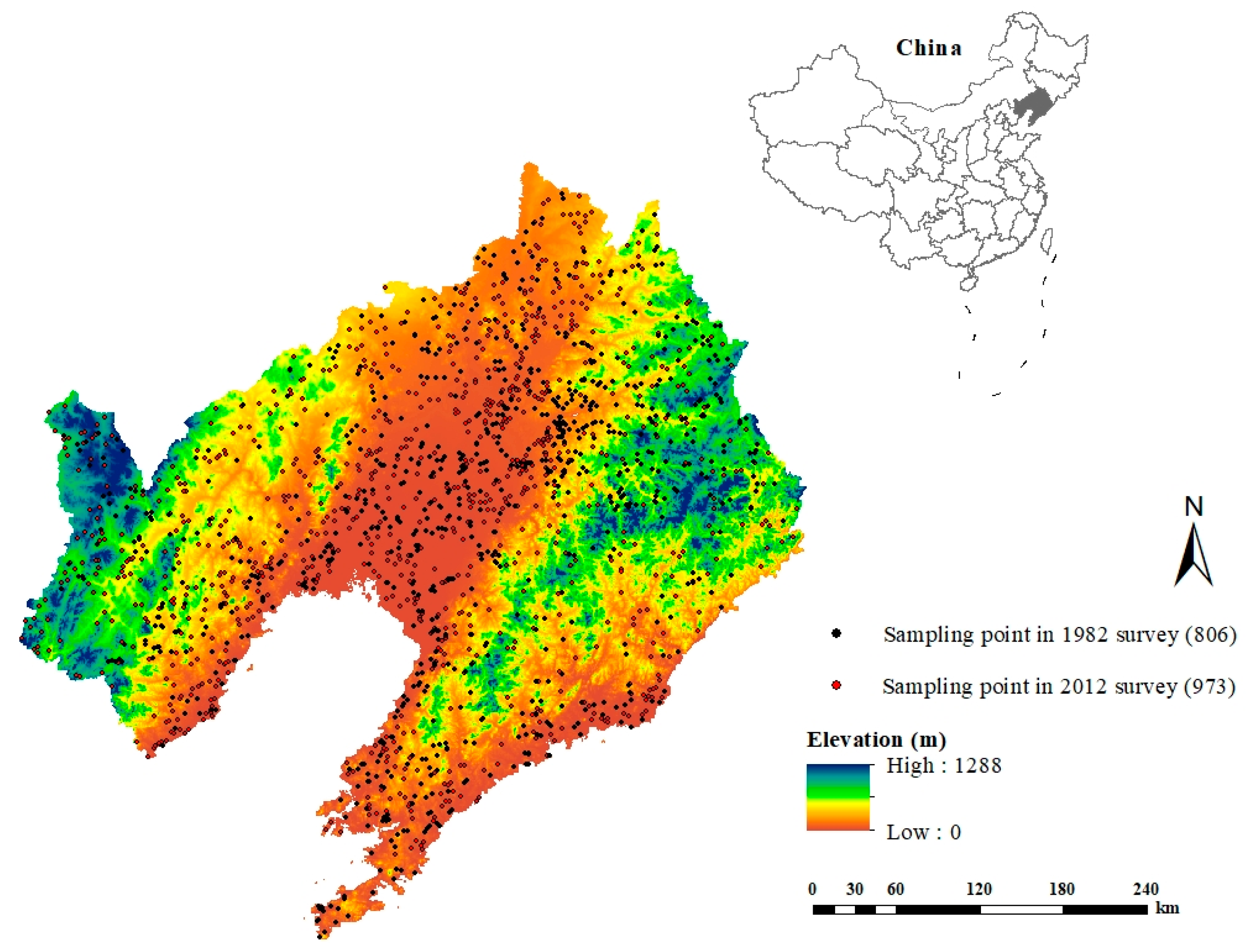
2.1. Study Area

Liaoning Province (118°–125° E, 38°–43° N) is located in the southernmost part of Northeast China, which belongs to temperate monsoon continental climate with a regional area of 140,000 km2 (Figure 1). Liaoning Province had a population of about 43 million in 2010. The gross domestic product of Liaoning Province in 2010 was 30.1 billion US dollars, ranking seventh among all provinces in China [28]. The terrain is generally high in the north and low in the south, inclining from land to sea. Mountains and hills are arranged on both sides of the east and west, inclining toward the central plain. Altitude varies from 0 m in coastal areas to 1332 m in eastern mountainous areas. The annual average precipitation ranges from 600 mm to 1100 mm, of which 65% is concentrated in summer and accompanied by high intensity rainstorms. The annual average temperature is 9 °C, the coldest and hottest temperature are January and July, and the temperatures are −40 °C and 30 °C, respectively. Variable topographic conditions result in different soil types. According to the classification of Chinese soil systems [29], the main soil types are Anthrosols and Cambisols, accounting for about 76% of the total area of the study area. Corresponding with the FAO-WRB classification system [30], the main soil types are Anthrosols and Cambisols. The main economic crops are Zea mays Linn., Oryza saliva subsp. keng, Glycine max, Malus domestica, Prunus persica var. nectarina, Cerasus pseudocerasus, and Vitis vinifera L.

2.2. Experimental Design

In this study, we first collected data, including soil survey data for 1982, environmental variables, and land-use data in two periods. Second, on the basis of collecting data, it was necessary to process the data, such as a unified coordinate system and spatial resolution of environmental variables. Third, the sampling scheme was designed by the purposeful sampling method, and then the soil samples were collected and analyzed in the whole study area. Finally, the appropriate model was selected to predict the spatial distribution of SOC and pH, and then the results were verified.

2.2.1. Soil Survey Data for 1982

Soil data in 1982 were obtained from Liaoning Province’s Second Soil Survey Office. The database includes 806 soil profiles covering all soil types and land types in the study area (Figure 1). The database includes soil physical and chemical properties, parent material information, tillage system, slope direction, slope gradient, landscape, and other information. This study limited the SOC and pH data of topsoil (0–20 cm) to 806 profiles.

2.2.2. Soil Sampling and Analysis

A total of 973 topsoil (0–20 cm) samples were collected in 2012 (Figure 1). In the total land area of Liaoning Province, the mountainous area is 88,000 km2, accounting for 59.5%. Thus, it is difficult to sample and analyze a large number of points and then map the distribution of SOC and pH across large areas, particularly in areas of rugged terrain. To represent the spatial characteristics of soil properties in complex geographical landscapes, a purposive sampling method was applied in this study [31]. Based on the pedogenesis of SOC and pH of the study area, elevation, MAT, MAP, and NDVI were the main environmental variables considered in collecting samples [2,6,14,23]. The specific location of each sampling point was recorded by a handheld global positioning system (GPS). A total of 1 kg of subsamples were collected at each sampling point for the subsequent determination of physical and chemical soil properties. In the Key Laboratory of Northeast Cultivated Land Conservation, Ministry of Agriculture of the People’s Republic of China, Shenyang Agricultural University, Shenyang, the SOC content was measured using a CN analyzer (Vario Max, Elementar Amerivas Ins., Germany) after air drying, removing litter, grinding, and sieving. Soil pH value was determined by an electronic acidity meter [6].

2.2.3. Environmental Variables

Ten selected environmental variables (elevation, slope gradient, topographic wetness index (TWI), mean annual temperature (MAT), mean annual precipitation (MAP), visible-red band 3 (B3), near-infrared band 4 (B4), short-wave infrared band 5 (B5), normalized difference vegetation index (NDVI), and land use) were used in this study to predict SOC and pH values. These variables were acquired through different channels and unified into the 90 m resolution raster data form in ArcGIS 10.1. Accordingly, sampling data and covariates are transformed into a united projection coordinate system (Universal Transverse Mercator) for modeling and analysis.
A 90 m resolution digital elevation model (DEM) captured from Shuttle Radar Topography Mission (SRTM) was used to generate elevation and slope gradient in ArcGIS 10.2, while TWI was carried out using the SAGA GIS software [32]. MAT and MAP are two mainly climatic variables which were obtained from the China Meteorological Data Service Center (http://data.cma.cn/en). Those climatic data covered the previous thirty years (1980–2010) and were derived as from 1 km grid from 673 meteorological stations in China (ArcGIS 10.2). The remote sensing data of the growing season of 1982 and 2012 (July to September) were obtained from the Computer Network Information Center of the Chinese Academy of Sciences. Remote sensing variables (B3, B4, and B5) were retained to represent the “organisms” soil forming factor. In addition, we have also chosen the NDVI to represent vegetation intensity.
Land use data (two periods) was in raster format and obtained from the National Science & Technology Infrastructure of China, National Earth System Science Data Sharing Infrastructure (http://www.geodata.cn). According to the China’s Second National Land Survey and Land Classification System, land use types were grouped into cultivated land, grassland, forest land, unutilized land, and other land-use types, including villages and rock outcrops, which were coded as 1, 2, 3, 4, and 5, respectively.

2.3. Random Forest Model

The RF model is a classical machine learning method [33]. It is widely used in the research of DSM. In the training process, the RF algorithm will generate multiple trees, and each tree is generated based on the initial training set [12]. All trees will grow to their maximum size without pruning branches. In the RF model, data are divided into “in-bag” and “out-of-pocket” for modeling and model validation [25,26], respectively. The average of the final prediction of all combinations is used as the prediction value of the RF model.
Three parameters of the RF model require users to define. They are the number of trees (ntree), number of random samples (mtry), and minimum size of data points (nodes) [23]. Normally ntree has a default value of 500, but we found it cannot provide robust predictions. So, we defined it as 1500 in our research. Mtry determines the model strength of each tree in the forest and the correlation between trees. With the increase of mtry, the intensity of each tree and the correlation between trees increases. For nodes, we use its default value of 5. The relative importance of predictive variables generated in the process of RF model prediction is estimated based on the average decline of predictive accuracy when the variables are arranged [26]. This relative importance is calculated to explain the percentage of total variance, which reflects the importance of variables to the predicted attributes [18]. In order to obtain the best and most stable prediction performance, we used the “Random Forest” package in R statistics software [34] to iterate the RF model 100 times and get its average value as the final prediction result.

2.4. Model Validation

Ten-fold cross-validation was used to evaluate the performance of the two-period RF model prediction in R statistics software. Four commonly used indices, i.e., mean absolute prediction error (MAE), root mean square error (RMSE), coefficient of determination (R2), and Lin’s concordance correlation coefficient (LCCC), were calculated [35]. These indices were defined as below:
M A E = 1 n i = 1 n | a i b i |
R M S E = 1 n i = 1 n ( a i b i ) 2
R 2 = i = 1 n ( a i b ¯ i ) 2 i = 1 n ( b i b ¯ i ) 2
L U C C = 2 r a b a 2 + b 2 + ( a ¯ + b ¯ ) 2
where a i , b i , a ¯ , and b ¯ are the predicted values, the observed values, the average values of the predicted, and the average values of the observed at site i , respectively; n is the number of samples; a and b are the variances of observed and predicted values; and r is the Pearson correlation coefficient.

3. Results

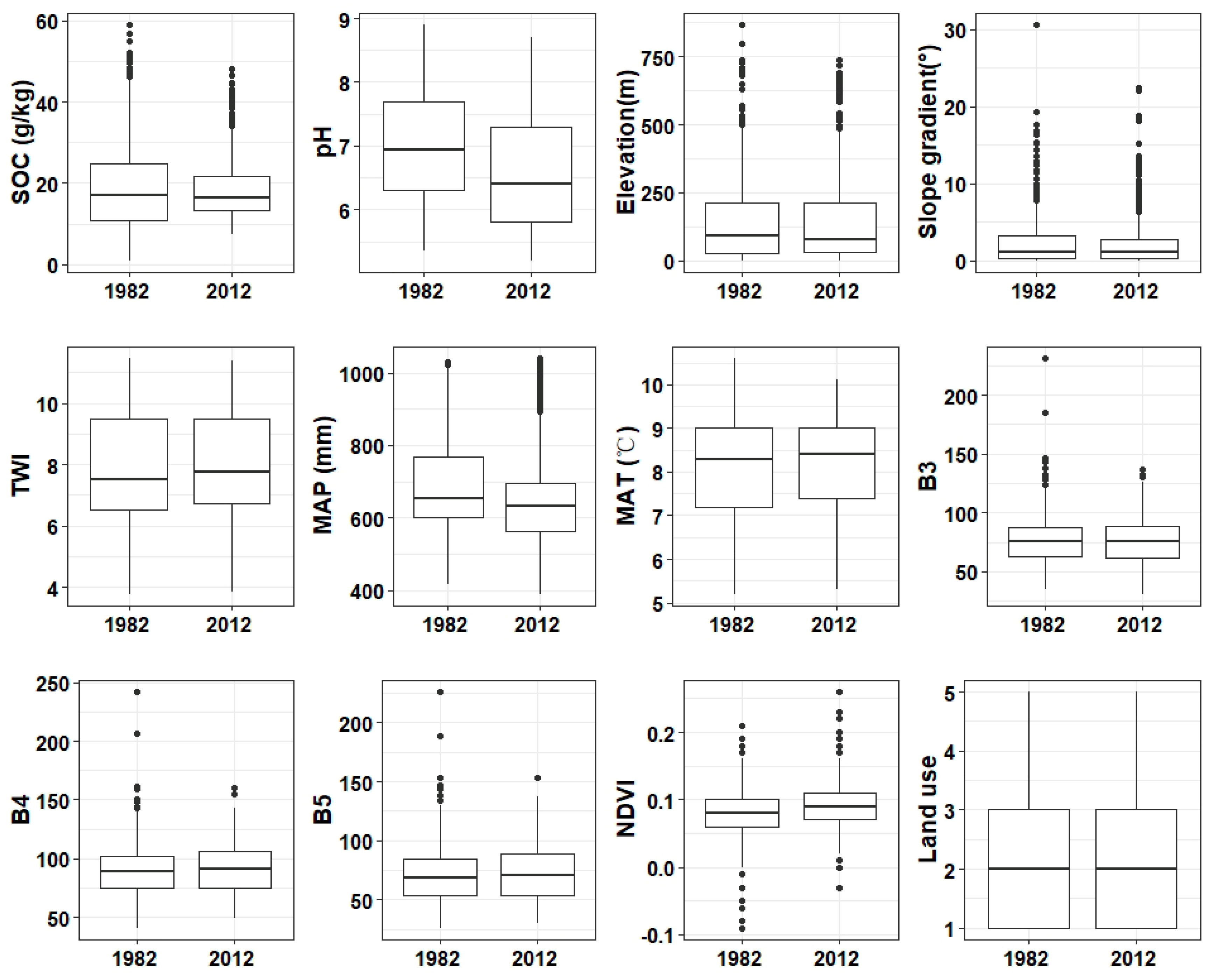
3.1. Descriptive Statistics

Figure 2 summarizes the descriptive statistics of SOC and pH measured during the two periods, as well as the values of the environmental variables at the sampling points. In 1982, the SOC and pH ranged from 0.94 g∙kg−1 to 58.93 g∙kg−1 and 5.35 to 8.90, respectively, with an average of 16.89 g∙kg−1 and 6.98. Average SOC and pH content in 2012 was 18.16 g∙kg−1 and 6.59, respectively. In 1982, the skewness coefficients of SOC and pH were 0.91 and 0.09, respectively. The data sets showed a generalized skewness distribution. The corresponding skewness coefficients of SOC and pH are 1.29 and 0.11 in 2012, respectively. Since SOC data did not conform to an orthogonal distribution, log transformation was performed to make the data conform to a normal distribution during two periods.
Table 1 lists the correlation coefficients of SOC and pH with selected environmental variables over two periods. Elevation, slope gradient, and MAP were positively correlated with SOC, while TWI, MAT, B3, B4, NDVI, and land use were negatively correlated with SOC in both periods. Correspondingly, TWI, MAT, NDVI, and land use were positively correlated with pH, but slope gradient and MAP were negatively correlated with pH during two periods. By studying Table 1, it was found that there are multiple collinearities among environmental variables. We believe that it was unreliable to predict the spatial distribution of SOC and pH by using the traditional statistical methods equation. Therefore, the RF method, which can avoid over-fitting and is relatively stable, was selected for spatial prediction.

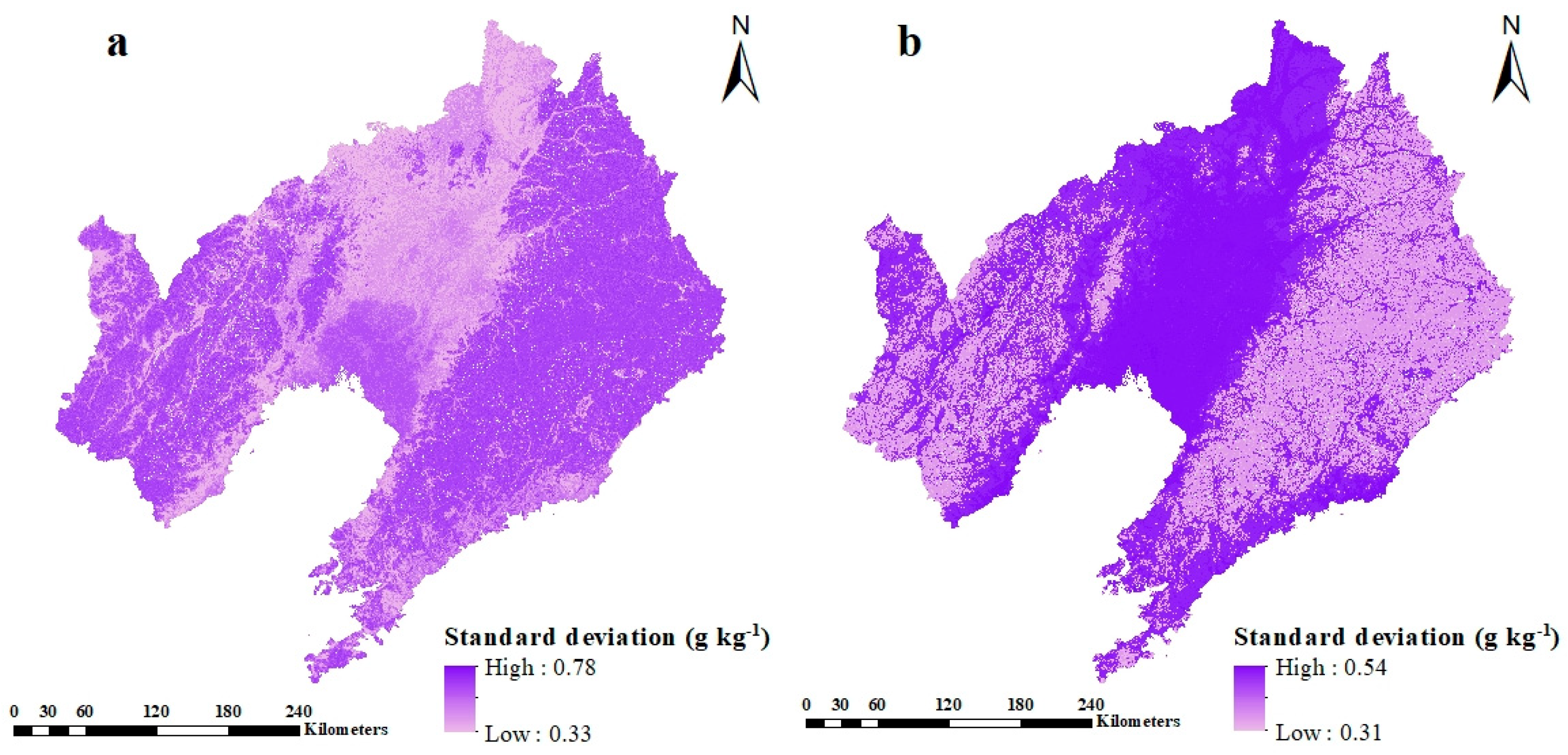
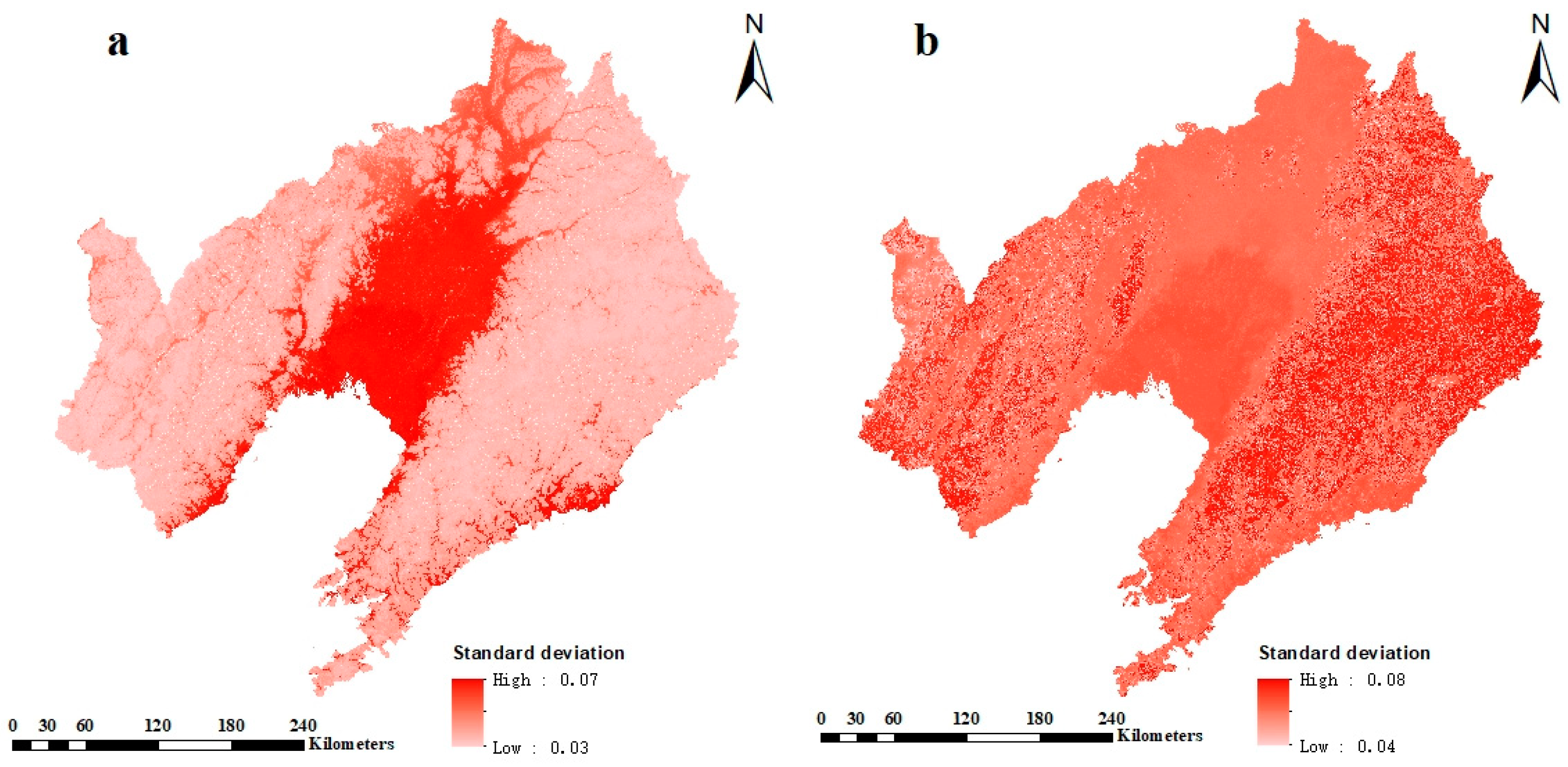
3.2. Uncertainties in the Present Study

The ten-fold cross-validation technique was selected to evaluate the predictive performance of SOC and pH using the RF model in two periods as shown in Table 2. Summary statistics showed that the RF model had systematically lower MAE and RMSE, and higher R2 and LUCC in the predictive quality of SOC and pH in both periods. The uncertainty of the RF model prediction is shown in Figure 3 and Figure 4. Both predictions had lower uncertainties with a mean SD of 0.55 g∙kg−1 and 0.06 for SOC and pH in 1982, respectively (Figure 3 and Figure 4). Correspondingly, the RF model also has low uncertainty, with the mean SD values of SOC and pH being 0.42 g∙kg−1 and 0.07 in 2012, respectively.

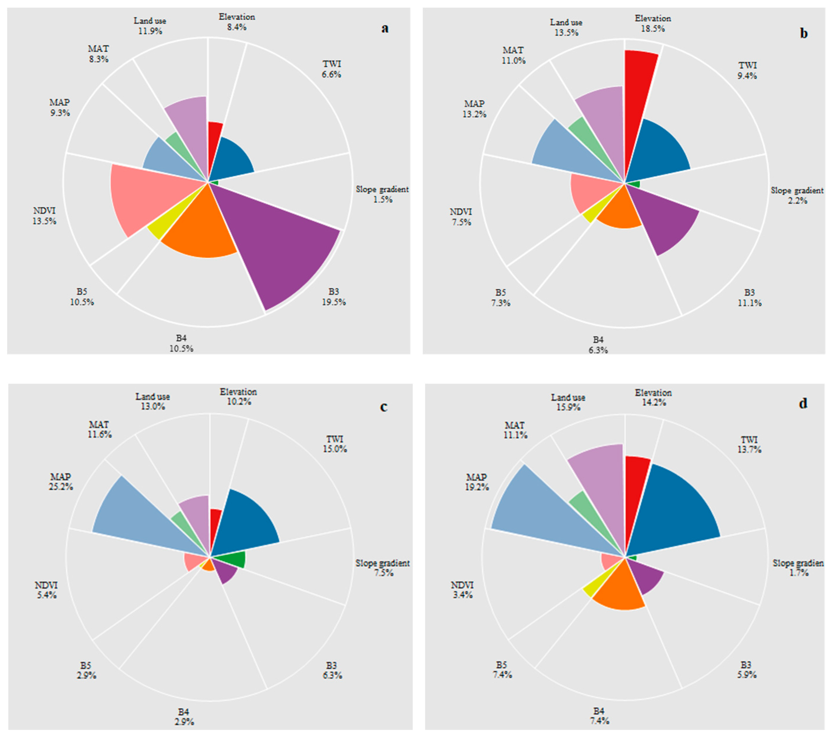
3.3. Importance of the Covariates

During the two study periods, the selected environmental variables showed different levels of importance in SOC and pH prediction (Figure 5). By repeating 100 simulations, the environmental variables of each model were standardized to 100% (Figure 5), and the relative importance (RI) of each environmental variable in the RF model was evaluated. In the process of SOC and pH prediction, the environmental variables of each variable showed different RI in two periods. Elevation, NDVI, and land use were three important variables affecting SOC distribution in both periods. Correspondingly, TWI and MAP were the key environmental variables affecting the spatial distribution of pH.

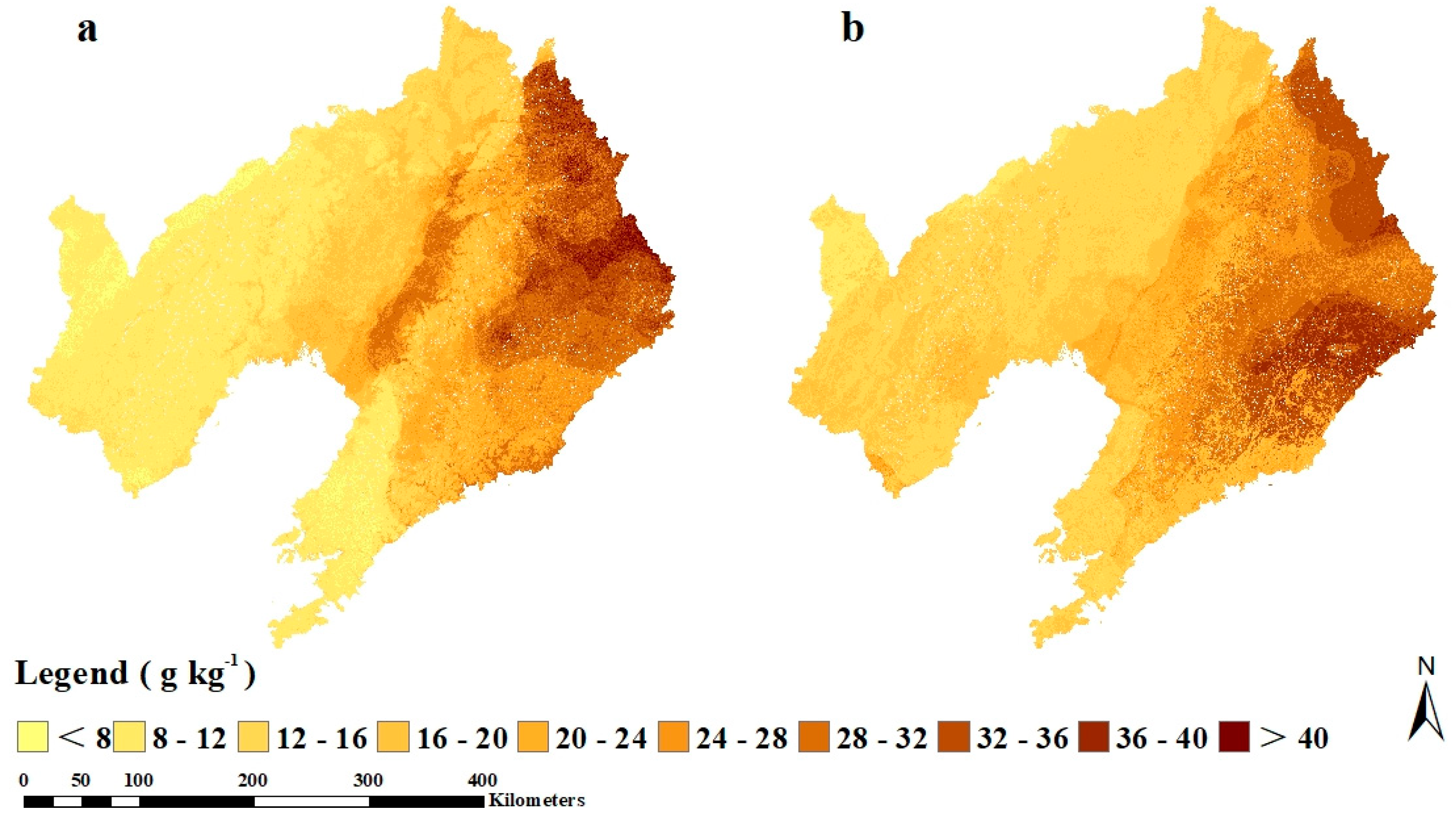
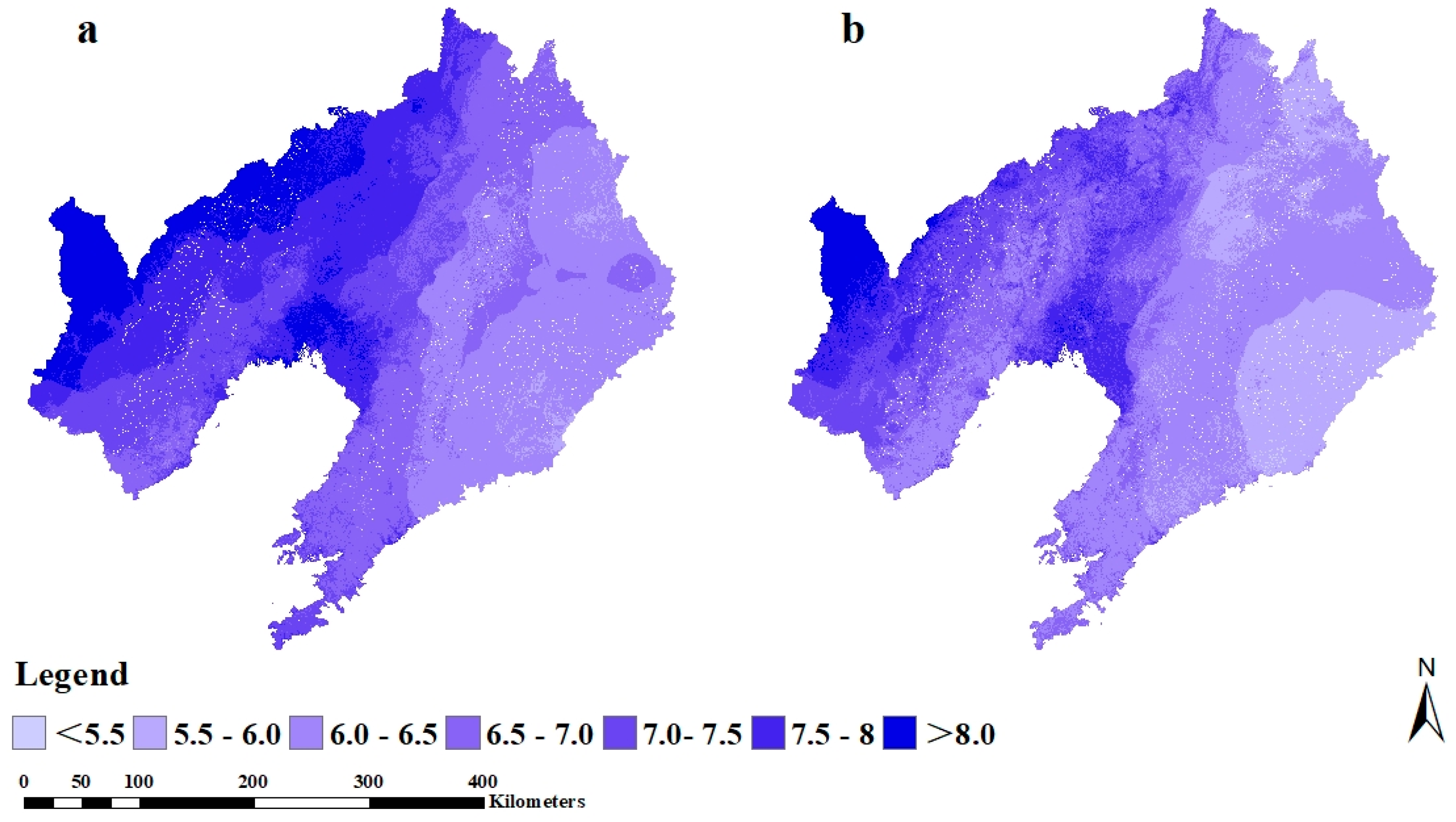
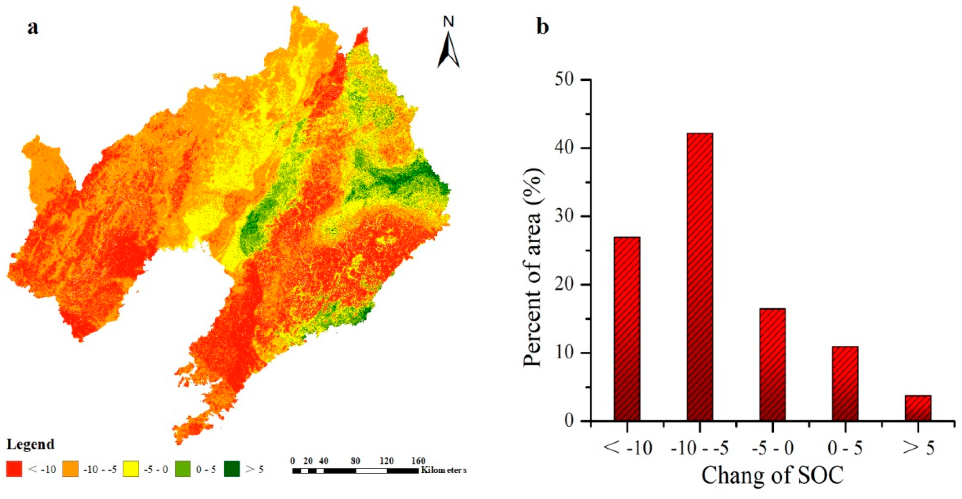
3.4. Spatial Prediction of SOC and pH

The RF model was selected and iterated 100 times to generate the spatial distribution maps of SOC and pH for 1982 and 2012 (Figure 6 and Figure 7). The average SOC content in 1982 (18.3 + 8.7 g∙kg−1) was higher than that in 2012 (16.7 + 7.1 g∙kg−1). Similarly, the average soil pH value in 1982 (7.1 + 0.7) was higher than that in 2012 (6.5 + 0.6). The percentage of change in area of SOC and pH at different levels is shown in Figure 8b and Figure 9b.
The spatial distribution of pH showed the opposite trend with SOC in both periods. For soil pH, it is an attribute produced in the process of soil formation, which is influenced by many natural and human factors. As far as the nature of the soil itself is concerned, the soil is neutral and acidic (5 < pH < 7.5), especially when it is neutral (6.5 < pH < 7.5), it is sensitive to the input of acidic substances. In 1982, the area of soil pH < 7.5 in Liaoning Province accounted for 51.3% of the total area, of which the area of 6.5 < pH < 7.5 was 39.2%. In 2012, the total area of cultivated land with soil pH < 7.5 accounted for 79.1%, of which the area of 6.5 < pH < 7.5 is 34.7%.
From 1982 to 2012, the SOC content showed a decreasing trend in the Liaoning Province, Northeast China. The average SOC content decreased from 18.34 g∙kg−1 in 1982 to 16.81 g∙kg−1 in 2012, and decreased by 1.53 g∙kg−1. SOC content in 85.43% of the study area decreased mainly in the central and eastern part of Liaoning Province, and the range of reduction was mainly between −10 g∙kg−1 and −5 g∙kg−1. Among them, 42.12% of the area of SOC content decreased, mainly distributed in the central plain area of Liaoning Province.
From the changes of the two periods, the soil in Liaoning Province showed a weak acidification trend in the past 30 years. The areas with serious acidification were mainly in the northwest and central regions. The area of acidification (pH < −2) was 15,118.9 km2, accounting for 10.6% of the total soil area. Weak acidification (−1 < pH < 0) is distributed in most areas of the province, with the largest area of 37,978.1 km2, accounting for 26.6% of the total area of land. 42.1% of the soil pH value increased, mainly distributed in the northwest and northeast of Liaoning Province, with an area of 60,219.5 km2 (Figure 8).

4. Discussion

4.1. Model Performance

The uncertainty of the RF model prediction is shown in Figure 3 and Figure 4. These results revealed that the RF model had excellent performance in predicting the spatial distribution of SOC and pH in 1982 and 2012. It was worth noting that there might be some uncertainties in this study, such as sampling error, experimental error, and simulation error. Although the environmental conditions, sampling strategies, and sampling methods in this study were different from previous studies, the performance of the RF model prediction was comparable to those studies. Were et al. [24] used the RF model to predict the SOC stocks in an Afromontane landscape, and concluded that the RF model could explain 52% of the spatial changes of SOC in this region. Yang et al. [23] used the RF model to interpret SOC in the northeastern margin of the Qinghai-Tibet Plateau. They found the model could explain 68% of the SOC changes in the region. A study in the Dano catchment (southwest Burkina Faso), Hounkpatin et al. [36] only explained 14% of SOC stocks variability using the RF model.

4.2. Effects of Covariates on SOC and pH

Topography, as one of the five major soil-forming factors, has a vital impact on soil moisture, temperature conditions, and spatial distribution of other soil-forming substances [17]. Therefore, spatial variability of soil properties was closely related to topographic factors [18,22]. In this study, it could be found that the topographic variables showed higher RI in 2012 (32% in 2012 and 19% in 1982). The results showed that topographic variables play the most important role in SOC spatial prediction in both periods. Altitude affects the microclimate in the region, forms different hydrothermal conditions, and indirectly affects microbial activity, which leads to the decomposition and transformation of SOM and the change of soil pH. This conclusion has been verified by Tsui et al. [37] and Martin et al. [38] in their research. In addition, TWI and the slope gradient of topographic variables were important environmental variables affecting the spatial variability of SOC in the established RF model (Figure 7 and Table 2). TWI takes into account the effects of topography and soil properties on soil moisture distribution, and plays an important role in the spatial distribution of SOC and pH [14].
Similarly, slope gradient also affected the movement of surface soil moisture and the loss of mineral carbon at the profile scale [18,19]. This conclusion has been confirmed in Denmark and China, respectively [22,24]. However, in Tsui’s research, it was pointed out that slope gradient had a negative impact on SOC spatial distribution, which could be attributed to the fact that there is lower vegetation productivity on steeper slopes, meaning less vegetation biomass on more sloping lands. In addition, there is less precipitation retention (more runoff) on these sloping areas and less moisture available for plant growth. At the same time, this is also often a result of erosion, both natural and man-made. In the process of soil erosion, most of the SOC will be displaced and redistributed along with the soil, resulting in a sharp decline in SOC, and some of the organic carbon will be mineralized in the process of erosion and released into the atmosphere in the form of CO2 [39]. The damage caused by moderate erosion and severe erosion is far greater than that caused by mild erosion. Compared with the soil that has not been eroded or slightly eroded, the SOC in the soil that has been eroded seriously decreases due to the loss of most organic carbon. Anderson et al. [39] studied the black calcareous soils in Saskatchewan, Canada, and found that 70% of soil organic carbon was lost on heavily eroded slopes, while only 40% of soil organic carbon was lost on slightly eroded slopes. Harden et al. [40] found that nearly 100% of the SOC had been lost after nearly 100 years of farmland cultivation near the Mississippi State, USA. They believed that 80% of the lost organic carbon was caused by soil erosion. For soil pH, higher salinity is likely due to higher erosion on sloping lands, removing less saline soil materials and exposing more saline subsurface materials. The main reasons can be explained as follows: Soil with high salinity has a low degree of development, low plant biomass, less humus, plant root and microbial hyphae, dispersed soil particles, and less aggregate, which results in a high soil erodibility and a large amount of soil erosion under the same rainfall intensity. Soils formed on acid parent rocks (such as granite and sandstone) generally have lower pH than those formed on limestone.
Climate variables had important effects on SOC and pH. Previous studies have shown that SOC and pH are significantly correlated with climate variables [18,23]. MAT and MAP are the most critical climate variables affecting the spatial distribution of SOC and pH in the region scale [18,23]. Previous studies had shown that elevation had an important impact on temperature and precipitation in microclimatic environment [14,23]. In this study, there was a highly significant and strong negative correlation among elevation, MAP, and MAT in the two periods (Table 2). Elevation was highly correlated with MAT and MAP, indicating that elevation might be a more important controlling factor than temperature and precipitation, so it could be used as a strong predictor of climate index and SOC status [14]. However, elevation also influences both natural and man-influenced soil erosion which directly affects SOC and pH. In high temperature and rainy areas, weathering and leaching are strong, salt base is easy to leach, and acid soil is easy to form [19]. However, in semi-arid or arid areas, the natural soil has less salt base leaching. On the contrary, because of the large evaporation of soil water, the salt-based substances in the lower layer tend to accumulate in the upper layer of the soil with the increase of capillary water, which makes the soil have a calcareous reaction [15,18].
Remote sensing variables were the main environmental variables affecting SOC in 1982, while in 2012 they were topography variables (Figure 5). NDVI (RI > 69%) had a high indicator capacity for topsoil SOC in Liaoning Province during 1982. Vegetation patterns and composition changes as land use and management changes, so too species change due to cropland replacing natural vegetation change (NDVI). Solid crop canopies due to crop cover would influence NVDI differently than native vegetation. This conclusion is consistent with previous studies [25,26]. Minasny et al. [41] revealed that NDVI was not only an outstanding predictor, but also played an active role in soil microbial activities, affecting the spatial distribution of SOC. NDVI had a low impact on the spatial distribution of SOC in 2012, mainly because a large number of forests, grasslands, and wetlands were converted to agricultural land from 1982 to 2012. Some studies [8,14,42] concluded that since China’s reform and opening up in the 1980s, land-use change has had a significant impact on the spatial change of SOC. The effect of vegetation on pH is mainly due to the selective absorption of ions by plant roots and the activity of soil microorganisms [2,9]. Soil under coniferous forests is beneficial to fungal growth, and the soil is acidic. In addition, the effect of artificial fertilization is more significant now. In the fields where acid fertilizers such as ammonium sulfate are often applied, the soil becomes acidic [16]. Among all remote sensing variables, NDVI and B3 were the key variables affecting SOC prediction in 2012. B4 and B5 could indirectly reflect the status of land use, so they could represent the spatial change of SOC under different land-use patterns. Wiesmeier et al. [43] and Adhikari and Hartemink [44] suggested that NDVI, B3, and B4 were the main predictors of SOC spatial distribution, which was consistent with our research. For soil pH, NDVI and B3 were the crucial remote sensing variables affecting its spatial distribution in 2012. In addition, the high spatial resolution remote sensing data could significantly improve the prediction performance of the model, which could be attributed to the fact that high-precision remote sensing data can better characterize the vegetation variation in the region.
Land use has a significant impact on SOC and pH by affecting soil properties and biomass production. Rapid changes in land use, such as the transition from forest to cultivation or grassland, have resulted in completely different soil environments in terms of soil moisture and temperature. It significantly affects the kinetics of organic matter accumulation and decomposition. Zhao et al. [45] reported that SOM increased the most in Jiangsu Province when dry land was changed into paddy fields in the past 26 years, which was 5.4 ± 3.9 g∙kg−1. From 1982 to 2012, SOC changed with land-use types. In the absence of land-use change, SOC has also undergone substantial changes. This can be attributed to a large number of crop production activities and human activities (building houses and roads, etc.), but no increase in soil biomass input. Zhao et al. [46] considered the profile characteristics of pH value and exchangeable acid of red soil under different vegetation types. It was concluded that acid-causing substances secreted by plant aboveground parts and roots could promote surface soil acidification through leaching and ion exchange. In addition, surface soil acidification also could be due to the use of acid forming fertilizers as land is converted to crop production. Guo et al. [47] showed that vegetation types could affect the movement of soil salt ions (i.e., Cl, SO2−4, CO2−3, HCO−3, Na+, K+, Mg2+, and Ca2+).

4.3. Estimates of SOC and pH

During these two periods, the spatial distribution of SOC showed a trend of low in the southwest and high in the east. The areas with high SOC content usually occurred under grassland and forest landscape units, which were usually less influenced by human beings. However, the areas with low SOC content mainly concentrated in low altitude plain areas, which were often disturbed by human activities. In 1982, we concluded that the spatial distribution pattern of SOC was closely related to the distribution of vegetation-related variables such as NDVI, which had been proved in recent studies [14,19,25]. Elbasiony et al. [48] revealed that vegetation affects SOM content by affecting the amount of vegetation litter entering the soil. In addition, the tillage also promoted OM oxidation of SOM/SOC. Surprisingly, the spatial distribution of SOC content in 2012 was also closely related to the topographic variables, especially elevation (Figure 5). Recent studies had demonstrated the effect of elevation on SOC [18,19,22,23]. Were et al. [24] concluded that SOC increased with altitude under an African mountainous landscape. Different elevation gradients affected SOC input and loss mainly through precipitation, temperature, and indirect control. Different altitudes can form different climatic zones, resulting in different precipitation and temperatures, thus indirectly affecting the input and loss of organic matter [14].
In 1982 and 2012, the spatial distribution pattern of pH was opposite to that of SOC. Soil pH is an attribute of soil formation, which is affected by many natural and human factors. This is mainly due to the input of acidic substances (mainly due to the use of acid-forming fertilizers and unreasonable planting and management methods) leading to the slow acidification of land soil. Overall, the area of land soil acidified in Liaoning Province has reached 82.1% in the past 30 years. In view of the present situation of land in Liaoning province, we need to improve management to reduce soil acidification. Emphasis is put on the use of soil acidifiers such as lime, calcium, magnesium, phosphorus, potassium, silicon, and chemical fertilizers, combined with straw returning and organic fertilizer application, which can effectively improve soil pH, improve soil aggregate structure and physical and chemical properties, improve the growth conditions of crop roots, and reduce soil acidification [1,6]. Less salt-based ion leaching and leaching of active aluminum in soil can reduce the activity of heavy metals in soil, thus improving the quality of cultivated land and crop yield and quality [2,9].
From 1982 to 2012, the SOC content showed a decreasing trend in the Liaoning Province, Northeast China. It is mainly distributed in the central plain area of Liaoning Province, which was the main commodity grain production area of Liaoning Province, with a long history of reclamation, leading to a significant reduction in SOC content. In Northeast China, Wang et al. [49] found that, with the increase of land reclamation years, the amount of SOC in topsoil decreased significantly. Their analysis showed that the mineralization rate of SOC after land reclamation was higher than that before reclamation, and the amount of SOC returned annually decreased with the increase of reclamation years. The increase of SOC content accounted for only 14.6% of the total study area, mainly distributed in the southwestern and southern coastal areas of Liaoning Province, which was closely related to the implementation of the policy of returning farmland to forestry and grassland in this region. In the southern coastal area of Liaoning Province, Wang et al. [14] used a BRT model to predict the soil organic carbon content in the two periods of the study area. They found that the area was characterized by carbon accumulation in the past 20 years, and pointed out that the policy of returning farmland to forestry was the main reason for the increase of SOC in this area.

5. Conclusions

We used the RF model to predict the spatial distribution characteristics of SOC and pH at two periods (1982 and 2012), based on which we determined the key environmental factors affecting their spatial-temporal changes. The results showed that the RF model was a powerful and effective DSM modeling method for predicting SOC and pH spatial patterns in both periods based on higher R2 and LUCC, and lower MAE and RMSE. Surprisingly, the spatial distribution patterns of SOC and pH presented opposite patterns in the two periods. Over the 30-year period, the mean SOC and pH decreased from 18.75 to 16.89 kg−1 and 6.98 to 6.59, respectively. The northeastern part of the study area had higher SOC levels than the rest of the area. We found elevation and NDVI were the two key variables affecting SOC distribution in both periods, while TWI and MAP was the main drivers affecting the spatial distribution of pH. Overall, this study mapped SOC and pH through DSM techniques with reasonable accuracy. Our findings from this study could promote ecological restoration, assist soil conservation, agricultural production planning, and environmental management in a more rational manner for Liaoning Province in northeastern China.

Author Contributions

S.W. and X.J. designed and developed the research idea; S.B., G.L., and Z.Y. collected and processed data; L.Q. and S.W. participated in drafting the manuscript; Q.Z. contributed to the scientific content and editing of the article; and all the authors revised and approved the manuscript.

Funding

The study is supported by the Fund Project of Shaanxi Key Laboratory of Land Consolidation (2019-ZD05).

Conflicts of Interest

The authors declare no conflict of interest.

References

  1. Dick, W.A. Organic Carbon, Nitrogen, and Phosphorus Concentrations and pH in Soil Profiles as Affected by Tillage Intensity 1. Soil Sci. Soc Am. J. 1982, 47, 102–107. [Google Scholar] [CrossRef]
  2. Yang, M.; Xu, D.; Chen, S.; Li, H.; Shi, Z. Evaluation of Machine Learning Approaches to Predict Soil Organic Matter and pH Using vis-NIR Spectra. Sensors 2019, 19, 263. [Google Scholar] [CrossRef] [PubMed]
  3. Power, J.F.; Prasad, R. Soil Fertility Management for Sustainable Agriculture; CRC Press: Boca Raton, FL, USA, 1997. [Google Scholar]
  4. Campbell, C.A. Soil organic carbon, nitrogen and fertility. Dev. Soil Sci. 1978, 8, 173–271. [Google Scholar]
  5. Tiessen, H.; Cuevas, E.; Chacon, P. The role of soil organic matter in sustaining soil fertility. Nature 1994, 371, 783. [Google Scholar] [CrossRef]
  6. Zaurov, D.E.; Perdomo, P.; Raskin, I. Optimizing soil fertility and pH to maximize cadmium removed by Indian mustard from contaminated soils. J. Plant Nutr. 1999, 22, 977–986. [Google Scholar] [CrossRef]
  7. Haynes, R.J.; Naidu, R. Influence of lime, fertilizer and manure applications on soil organic matter content and soil physical conditions: A review. Nutr. Cycl. Agroecosyst. 1998, 51, 123–137. [Google Scholar] [CrossRef]
  8. Sun, B.; Zhou, S.; Zhao, Q. Evaluation of spatial and temporal changes of soil quality based on geostatistical analysis in the hill region of subtropical China. Geoderma 2003, 115, 85–99. [Google Scholar] [CrossRef]
  9. Tu, C.; He, T.; Lu, X.; Luo, Y.; Smith, P. Extent to which pH and topographic factors control soil organic carbon level in dry farming cropland soils of the mountainous region of Southwest China. Catena 2018, 163, 204–209. [Google Scholar] [CrossRef]
  10. Goudie, A.S. Human Impact on the Natural Environment; John Wiley & Sons: Hoboken, NJ, USA, 2018. [Google Scholar]
  11. Vågen, T.G.; Winowiecki, L.A.; Tondoh, J.E.; Desta, L.T.; Gumbricht, T. Mapping of soil properties and land degradation risk in Africa using MODIS reflectance. Geoderma 2016, 263, 216–225. [Google Scholar] [CrossRef] [Green Version]
  12. Hengl, T.; Heuvelink, G.B.; Kempen, B.; Leenaars, J.G.; Walsh, M.G.; Shepherd, K.D.; Tondoh, J.E. Mapping soil properties of Africa at 250 m resolution: Random forests significantly improve current predictions. PLoS ONE 2015, 10, e0125814. [Google Scholar] [CrossRef]
  13. Minasny, B.; McBratney, A.B. Digital soil mapping: A brief history and some lessons. Geoderma 2016, 264, 301–311. [Google Scholar] [CrossRef]
  14. Wang, S.; Wang, Q.; Adhikari, K.; Jia, S.; Jin, X.; Liu, H. Spatial-temporal changes of soil organic carbon content in Wafangdian, China. Sustainability 2016, 8, 1154. [Google Scholar] [CrossRef]
  15. Rosemary, F.; Indraratne, S.P.; Weerasooriya, R.; Mishra, U. Exploring the spatial variability of soil properties in an Alfisol soil catena. Catena 2017, 150, 53–61. [Google Scholar] [CrossRef]
  16. Pahlavan-Rad, M.R.; Akbarimoghaddam, A. Spatial variability of soil texture fractions and pH in a flood plain (case study from eastern Iran). Catena 2018, 160, 275–281. [Google Scholar] [CrossRef]
  17. Jenny, H. Factors of Soil Formation: A System of Quantitative Pedology; McGrawHill: New York, NY, USA, 1994. [Google Scholar]
  18. Wang, S.; Jin, X.; Adhikari, K.; Li, W.; Yu, M.; Bian, Z.; Wang, Q. Mapping total soil nitrogen from a site in northeastern China. Catena 2018, 166, 134–146. [Google Scholar] [CrossRef]
  19. Malone, B.P.; Jha, S.K.; Minasny, B.; McBratney, A.B. Comparing regression-based digital soil mapping and multiple-point geostatistics for the spatial extrapolation of soil data. Geoderma 2016, 262, 243–253. [Google Scholar] [CrossRef]
  20. Behrens, T.; Schmidt, K.; MacMillan, R.A.; Rossel, R.A.V. Multi-scale digital soil mapping with deep learning. Sci. Rep. 2018, 8. [Google Scholar] [CrossRef]
  21. Jafari, R.; Sharifi, F.; Bagherpour, B.; Safari, M. Prevalence of intestinal parasites in Isfahan city, central Iran, 2014. J. Parasit. Dis. 2016, 40, 679–682. [Google Scholar] [CrossRef]
  22. Minasny, B.; Setiawan, B.I.; Arif, C.; Saptomo, S.K.; Chadirin, Y. Digital mapping for cost-effective and accurate prediction of the depth and carbon stocks in Indonesian peatlands. Geoderma 2016, 272, 20–31. [Google Scholar]
  23. Yang, R.M.; Zhang, G.L.; Liu, F.; Lu, Y.Y.; Yang, F.; Yang, F.; Li, D.C. Comparison of boosted regression tree and random forest models for mapping topsoil organic carbon concentration in an alpine ecosystem. Ecol. Indic. 2016, 60, 870–878. [Google Scholar] [CrossRef]
  24. Were, K.; Bui, D.T.; Dick, Ø.B.; Singh, B.R. A comparative assessment of support vector regression, artificial neural networks, and random forests for predicting and mapping soil organic carbon stocks across an Afromontane landscape. Ecol. Indic. 2015, 52, 394–403. [Google Scholar] [CrossRef]
  25. Belgiu, M.; Drăguţ, L. Random forest in remote sensing: A review of applications and future directions. ISPRS J. Photogramm. Remote Sens. 2016, 114, 24–31. [Google Scholar] [CrossRef]
  26. Kim, J.; Grunwald, S. Assessment of carbon stocks in the topsoil using random forest and remote sensing images. J. Environ. Qual. 2016, 45, 1910–1918. [Google Scholar] [CrossRef] [PubMed]
  27. Zhang, Q.; He, H.S.; Liang, Y.; Hawbaker, T.J.; Henne, P.D.; Liu, J.; Huang, C. Integrating forest inventory data and MODIS data to map species-level biomass in Chinese boreal forests. Can. J. For. Res. 2018, 48, 461–479. [Google Scholar] [CrossRef]
  28. Bureau of Statistics Liaoning Province. Statistical Yearbook of Liaoning 2011; China Statistics Press: Beijing, China, 2011. (In Chinese)
  29. Gong, Z.T. Chinese Soil Taxonomy; Science Press: Beijing, China, 1999; p. 903. [Google Scholar]
  30. FAO (Food and Agriculture Organization). International Soil Classification System for Naming Soil and Creating Legends for Soil Maps; Food and Agriculture Organization: Rome, Italy, 2014. [Google Scholar]
  31. Zhu, A.X.; Yang, L.; Li, B.; Qin, C.; English, E.; Burt, J.E.; Zhou, C. Purposive sampling for digital soil mapping for areas with limited data. In Digital Soil Mapping with Limited Data; Hartemink, A.E., McBratney, A., de Lourdes Mendonça-Santos, M., Eds.; Springer: Berlin/Heidelberg, Germany, 2008; pp. 33–245. [Google Scholar]
  32. Conrad, O.; Bechtel, B.; Bock, M.; Dietrich, H.; Fischer, E.; Gerlitz, L.; Böhner, J. System for automated geoscientific analyses (SAGA) v. 2.1. 4. Geosci. Model Dev. 2015, 8, 1991–2007. [Google Scholar] [CrossRef]
  33. Grimm, R.; Behrens, T.; Märker, M.; Elsenbeer, H. Soil organic carbon concentrations and stocks on Barro Colorado Island—Digital soil mapping using Random Forests analysis. Geoderma 2008, 146, 102–113. [Google Scholar] [CrossRef]
  34. R Development Core Team. R: A Language and Environment for Statistical Computing. R Foundation for Statistical Computing, 2013, Vienna, Austria. Available online: https://www.rproject.org/ (accessed on 7 March 2013).
  35. Lin, L. A concordance correlation coefficient to evaluate reproducibility. Biometrics 1989, 45, 255–268. [Google Scholar] [CrossRef]
  36. Hounkpatin, H.O.; Boyce, C.J.; Dunn, G.; Wood, A.M. Modeling bivariate change in individual differences: Prospective associations between personality and life satisfaction. J. Pers. Soc. Psychol. 2018, 115, e12. [Google Scholar] [CrossRef]
  37. Tsui, C.C.; Tsai, C.C.; Chen, Z.S. Soil organic carbon stocks in relation to elevation gradients in volcanic ash soils of Taiwan. Geoderma 2013, 209, 119–127. [Google Scholar] [CrossRef]
  38. Martin, M.P.; Orton, T.G.; Lacarce, E.; Meersmans, J.; Saby, N.P.A.; Paroissien, J.B.; Joliveta, C.; Boulonnea, L.; Arrouays, D. Evaluation of modelling approaches for predicting the spatial distribution of soil organic carbon stocks at the national scale. Geoderma 2014, 223, 97–107. [Google Scholar] [CrossRef]
  39. Anderson, D.W.; De Jong, E.; Verity, G.E.; Gregorich, E.G. The effects of cultivation on the organic matter of soils of the Canadian prairies. In Transactions of the XIII Congress of International Society of Soil Science; Reclam Verlag: Hamburg, Germany, 1986; Volume 7, pp. 1344–1345. [Google Scholar]
  40. Harden, J.W.; Sharpe, J.M.; Parton, W.J.; Ojima, D.S.; Fries, T.L.; Huntington, T.G.; Dabney, S.M. Dynamic replacement and loss of soil carbon on eroding cropland. Glob. Biogeochem. Cycles 1999, 13, 885–901. [Google Scholar] [CrossRef]
  41. Minasny, B.; McBratney, A.B.; Malone, B.P.; Wheeler, I. Digital mapping of soil carbon. Adv. Agron. 2013, 118, 4. [Google Scholar]
  42. Wang, S.; Zhuang, Q.; Jia, S.; Jin, X.; Wang, Q. Spatial variations of soil organic carbon stocks in a coastal hilly area of China. Geoderma 2018, 314, 8–19. [Google Scholar] [CrossRef]
  43. Wiesmeier, M.; Hübner, R.; Spörlein, P.; Geuß, U.; Hangen, E.; Reischl, A.; Kögel-Knabner, I. Carbon sequestration potential of soils in southeast Germany derived from stable soil organic carbon saturation. Glob. Change Boil. 2014, 20, 653–665. [Google Scholar] [CrossRef] [PubMed]
  44. Adhikari, K.; Hartemink, A.E. Digital mapping of topsoil carbon content and changes in the Driftless Area of Wisconsin, USA. Soil Sci. Soc Am. J. 2015, 79, 155–164. [Google Scholar] [CrossRef]
  45. Zhao, M.S.; Zhang, G.L.; Wu, Y.J.; Li, D.C.; Zhao, Y.G. Driving forces of soil organic matter change in Jiangsu Province of China. Soil Use Manag. 2015, 31, 440–449. [Google Scholar] [CrossRef]
  46. Zhao, K.L.; Cai, Z.J.; Wang, B.J. Changes in pH and exchangeable acidity at depths of red soils derived from 4 parent materials under 3 vegetations. Sci. Agric. Sin. 2015, 28, 2818–2826. (In Chinese) [Google Scholar]
  47. Guo, Q.E.; Wang, Y.Q.; Ma, Z.M.; Guo, T.; Che, Z.; Huang, G.; Nan, L. Effect of vegetation types on soil salt ions transfer and accumulation in soil profile. Sci. Agric. Sin. 2011, 44, 2711–2729. (In Chinese) [Google Scholar]
  48. Elbasiouny, H.; Abowaly, M.; Abu_Alkheir, A.; Gad, A. Spatial variation of soil carbon and nitrogen pools by using ordinary Kriging method in an area of north Nile Delta, Egypt. Catena 2014, 113, 70–78. [Google Scholar] [CrossRef]
  49. Wang, Y.; Wang, S.; Adhikari, K.; Wang, Q.; Sui, Y.; Xin, G. Effect of cultivation history on soil organic carbon status of arable land in northeastern China. Geoderma 2019, 342, 55–64. [Google Scholar] [CrossRef]
Figure 1. Map of the sampling sites in Liaoning Province for the 1982 and 2012 surveys.
Sustainability 11 03569 g001
Figure 2. Boxplots of SOC and pH values in 1982 and 2012 derived for different environmental variables. SOC, Soil Organic Carbon; TWI, topographic wetness index; MAP, mean annual precipitation; MAT, mean annual temperature; B3, Landsat TM band 3; B4, Landsat TM band 4; B5, Landsat TM band 5; and NDVI, Normalized Difference Vegetation Index.
Sustainability 11 03569 g002
Figure 3. Standard deviation of SOC predicted by the random forest (RF) model in the (a) 1982 and (b) 2012 surveys.
Sustainability 11 03569 g003
Figure 4. Standard deviation of pH predicted by the random forest (RF) model in the (a) 1982 and (b) 2012 surveys.
Sustainability 11 03569 g004
Figure 5. Relative importance of each variable as determined from 100 runs of the random forest (RF) for SOC in 1982 (a) and 2012 (b) and pH in 1982 (c) and 2018 (d), which are shown in decreasing order and normalized to 100%. TWI, topographic wetness index; MAP, mean annual precipitation; MAT, mean annual temperature; B3, Landsat TM band 3; B4, Landsat TM band 4; B5, Landsat TM band 5; and NDVI, Normalized Difference Vegetation Index.
Sustainability 11 03569 g005
Figure 6. Mean spatial distribution maps of SOC predicted by the RF model in (a) 1982 and (b) 2012.
Sustainability 11 03569 g006
Figure 7. Mean spatial distribution maps of pH predicted by the RF model in (a) 1982 and (b) 2012 surveys.
Sustainability 11 03569 g007
Figure 8. Spatial distributions of SOC change (a) and area percentages of SOC (b) at different levels between the 1982 and 2012 surveys.
Sustainability 11 03569 g008
Figure 9. Spatial distributions of pH change (a) and area percentages of pH (b) at different levels between the 1982 and 2012 surveys.
Sustainability 11 03569 g009
Table 1. Relationships between observed SOC (g∙kg−1) and pH with all predictors in the 1982 and 2012 surveys.
YearPropertySOCpHElevationSlope GradientTWIMAPMATB3B4B5
1982pH−0.36 **
Elevation0.25 **−0.12 **
Slope gradient0.12 **−0.19 **0.48 **
TWI−0.12 **0.32 **−0.54 **−0.70 **
MAP0.62 **−0.65 **0.25 **0.19 **−0.24 **
MAT−0.58 **0.27 **−0.58 **−0.19 **0.21 **−0.37 **
B3−0.11 **0.034−0.14 **−0.17 **0.05−0.15 **0.14 **
B4−0.24 **0.07 *−0.17 **−0.19 **0.05−0.25 **0.24 **0.97 **
B5−0.21 **0.05−0.10 **−0.15 **−0.01−0.23 **0.18 **0.94 **0.98 **
NDVI−0.42 **0.16 **−0.11 **−0.070.01−0.32 **0.36 **−0.31 **−0.06−0.06
Land use−0.38 **0.24 **−0.17−0.24 *−0.31 **−0.150.11−0.34 **−0.09−0.07
2012pH−0.29 **
Elevation0.18 **0.23 **
Slope gradient0.12 **−0.10 **0.44 **
TWI−0.11 **0.19 **−0.55 **−0.72 **
MAP0.59 **−0.52 **−0.24 **0.12 **−0.12 **
MAT−0.36 **0.11 **−0.42 **−0.13 **0.15 **−0.21 **
B3−0.06−0.07 *−0.06−0.12 **0.09 **−0.12 **0.08 *
B4−0.15 **−0.05−0.05−0.12 **0.06−0.21 **0.17 **0.97 **
B5−0.14 **−0.06−0.02−0.10 **0.02−0.20 **0.13 **0.95 **0.98 **
NDVI−0.33 **0.11 **0.07 *0.01−0.11 **−0.32 **0.32 **−0.34 **−0.12 **−0.11 **
Land use−0.32 **0.21 **−0.12−0.23 *−0.29 **−0.160.17−0.31 **−0.05−0.08
Note: p < 0.05 shown in “*”; p < 0.01 shown in “**”. TWI, topographic wetness index; MAP, mean annual precipitation; MAT, mean annual temperature; B3, Landsat TM band 3; B4, Landsat TM band 4; B5, Landsat TM band 5; and NDVI, Normalized Difference Vegetation Index.
Table 2. Summary statistics of the predictive quality of the random forest (RF) model in 1982 and 2012 for SOC and pH prediction with 100 runs.
PropertyYearIndexMinMedianMeanMax
SOC1982MAE4.234.344.354.41
RMSE5.615.625.715.82
R20.630.680.690.71
LCCC0.810.810.810.83
2012MAE3.213.253.263.29
RMSE4.314.384.394.43
R20.580.620.630.64
LCCC0.750.780.790.81
pH1982MAE0.460.470.470.47
RMSE0.580.580.580.59
R20.520.540.540.55
LCCC0.710.720.720.72
2012MAE0.520.530.530.53
RMSE0.660.670.670.67
R20.480.480.480.49
LCCC0.660.660.660.67
Note: MAE, the mean error; RMSE, root mean squared error; R2 coefficient of determination; and LCCC, Lin’s concordance correlation coefficient were used to evaluate accuracy.

