Efficient Energy Management in a Microgrid with Intermittent Renewable Energy and Storage Sources


1
Department of Electrical and Computer Engineering, King Abdulaziz University, Jeddah 21589, Saudi Arabia
2
Department of Electrical Engineering, Hafr Al-Batin University, Hafr Al-Batin 31991, Saudi Arabia
*
Author to whom correspondence should be addressed.
Sustainability 2019, 11(14), 3839; https://0-doi-org.brum.beds.ac.uk/10.3390/su11143839
Submission received: 23 June 2019
/
Revised: 11 July 2019
/
Accepted: 12 July 2019
/
Published: 14 July 2019
(This article belongs to the Section Energy Sustainability)
Abstract
:Substituting a single large power grid into various manageable microgrids is the emerging form for maintaining power systems. A microgrid is usually comprised of small units of renewable energy sources, battery storage, combined heat and power (CHP) plants and most importantly, an energy management system (EMS). An EMS is responsible for the core functioning of a microgrid, which includes establishing continuous and reliable communication among all distributed generation (DG) units and ensuring well-coordinated activities. This research focuses on improving the performance of EMS. The problem at hand is the optimal scheduling of the generation units and battery storage in a microgrid. Therefore, EMS should ensure that the power is shared among different sources following an imposed scenario to meet the load requirements, while the operational costs of the microgrid are kept as low as possible. This problem is formulated as an optimization problem. To solve this problem, this research proposes an enhanced version of the most valuable player algorithm (MVPA) which is a new metaheuristic optimization algorithm, inspired by actual sporting events. The obtained results are compared with numerous well-known optimization algorithms to validate the efficiency of the proposed EMS.
1. Introduction
The alarming rise in carbon emissions means production of clean energy is required urgently. The recent incorporation of both large and small renewable energy sources into the existing power system is a positive step towards decarbonizing our power generation, however, much effort is still required to address the challenges directly associated with widespread penetration of such energy sources. In addition to reducing carbon emissions, these efforts are primarily targeted to produce a sustainable energy supply.
Location-based renewable energy sources have naturally become an alternative power source within the microgrid, which is constituted of distributed generation (DG) units, storage devices, and loads. There is a tendency for the microgrid to operate in both islanded and grid-connected modes. Determining an optimal share of power produced by available DGs in a microgrid is a challenge and has remained one of the most interesting and important topics of research.
In literature, various performance attributes of microgrids were optimized using different optimization algorithms. Power generation scheduling was optimized in [1] using an artificial fish swarm algorithm (AFSA), whereas, in [2], day-a-head optimized scheduling was presented using a harmony search (HS) and differential evolution (DE) algorithms. Reference [3] solved the economic power dispatch using four algorithms, namely, the direct search method, particle swarm optimization (PSO), lambda logic, and lambda iteration. In reference [4], additive-increase-multiplicative-decrease algorithms were used to optimize power sharing among active DGs. In order to determine the optimal component sizing in a microgrid, the mixed integer linear programming (MILP) method has been used to model the microgrid components with consideration of demand response [5]. In another study [6], similar sizing problems of microgrid components were solved using a genetic algorithm (GA) and the energy management issue was formulated using MILP. In addition to component sizing, system configuration was optimized in [7] using the multi-objective PSO by taking into account production cost, reliability, and environmental impact. The studied system comprised of a diesel generator, solar panels, wind turbines, and battery storage. Several methods have also been used for optimizing multi variable problems of energy management systems (EMS) in microgrids [8,9,10,11,12,13]. Wang et al. [14] investigated EMS of a microgrid with multi period optimization problems using an MPI based PSO algorithm and concluded that the proposed algorithm could be effectively used to improve the operation time.
Four techniques were used in [15] to determine the optimized operational strategy for an entire day based on least operating cost and minimum carbon emissions. These techniques were a non-dominated sorting genetic algorithm (NSGA), multi-objective PSO, multi-objective uniform water cycle algorithm (WCA), and normal constraint algorithm. Reference [16] presented a real time EMS that had the tendency to optimally minimize carbon emissions and energy cost, and simultaneously maximized the power coming from renewable DGs using binary PSO. An improved binary PSO with double-structure coding was applied to optimize a microgrid operation [17]. In this research, the effectiveness of the proposed algorithm was verified based on the simulation results. Another real time EMS was also proposed by applying multi-objective PSO for an islanded microgrid [18]. Compared with a multi objective GA, the proposed algorithm creates faster computation. A multi-objective PSO algorithm was later modified to optimize the operation of the system with minimum energy consumption, cost, and emissions [19]. It was found that the proposed multi-objective PSO could be validated for multi variable EMS of a factory. The optimal power control strategy for a standalone microgrid was developed and presented in [20] where optimized gains of a proportional-integrator controller of inverter-based DGs using hybrid big bang-big crunch (BB–BC) algorithm were found.
With the aim of adjusting microgrid generation to energy demand, numerous technical studies have been carried out to improve energy management with penetration of renewable energy sources combined with energy storage devices in microgrids [21,22,23,24,25]. Alvarez et al. [26] conducted an optimization of micro sources in a DG microgrid in terms of emission and fuel consumption costs. This work showed a faster response of microgrid management with better micro source stability and global cost. Another study, [27], evaluated optimal energy management in an isolated microgrid with renewable energy sources (i.e., PV and wind power plants) using pumped-storage and demand response. Through this research, technical and economic performances of the system were significantly improved by implementing demand response and optimal scheduling of the pumped-storage. Kim et al. [28] evaluated the acceptability and stability of a hybrid microgrid system to provide power supply for Gasado Island in South Korea. It showed that the system is not only stable but also capable of predicting the electricity supply and demand, managing the batteries charge/discharge, and controlling the distributed generators with lower costs and higher renewable energy fraction. Meanwhile, a technical analysis of a hybrid system was performed for electricity shortage conditions caused by a disaster [29]. The hybrid system is off-grid and consists of conventional and renewable energy sources and energy storage system. As a result, the renewable energy sources can provide backup power supply in the absence of conventional energy sources during disaster. The authors in another study [30] analyzed optimal energy management of a renewable-based microgrid using a PSO algorithm combined with a primal-dual interior point and concluded that the proposed robust model effectively solved the microgrid energy management problems by minimizing operation costs and satisfying the PVs insolation limitation and the microgrid physical constraints.
In reference [31], a robust management system was proposed for a microgrid in the presence of high penetration of renewable DGs. This system tended to minimize the microgrid’s running and worst-case transaction costs, along with the utility of the dispatchable loads while considering the stochastic nature of DGs. Reference [32] presented a model for stochastic microgrid energy scheduling with the primary goal of minimizing anticipated running costs and power losses. Plug-in electric vehicles, storage devices, and DGs were taken into consideration while modeling the microgrid. In another study [33], several forecasting methods were applied to optimize the EMS of distributed energy resources. In reference [34], the charging and discharging rates of batteries were controlled to optimize energy management in a microgrid constituted of renewable energy sources and storage devices. For optimal energy management, a drop-based controller was utilized, whereas, for power distribution among charging stations, an aggregator was used. Ultimately the power was distributed among charging stations subjected to their droop participation. The Markov decision process (MDP) was used to formulate multi-energy systems scheduling in [35], where the decision space and large state of MDP were solved using a rollout algorithm. Wind power, batteries, and combined heat and power (CHP) were used to model a microgrid in grid connected mode. Reference [36] proposed a memory-based GA to minimize costs by optimally distributing power among DGs connected in a microgrid. An algorithm was implemented on the microgrid consisting of solar plants, wind plants, and CHP. Chen et al. [37] evaluated a mutual dependency of cogeneration units and proposed a direct search method to solve the CHP dispatch problem. A number of studies have been done to verify the proposed approach. Another study [38] analyzed the effect of distributed energy resources integration in an industrial microgrid and proposed a model with onsite generation, i.e., CHP and a wind turbine, which was applied to a manufacturing facility. In a recent study [39], optimization of energy, heat, and demand in a microgrid was conducted using a mathematical model based on MILP with the aim of minimizing the operational cost.
In this paper, we propose an efficient energy management system (EEMS) for the optimal scheduling of different sources in a microgrid, considering the intermittent behavior of renewable energy sources, with and without storage resources. The developed system can efficiently manage the energy under different scenarios. This EEMS uses an enhanced version of the most valuable player algorithm (EMVPA) to minimize the operating cost of the microgrid.
The remainder of this paper is organized as follows. The investigated microgrid is introduced in Section 2. The details of the energy management strategy are described in Section 3. The problem formulation for minimizing operating cost is presented in Section 4 and the optimization algorithms are proposed in Section 5. Results and discussion are provided in Section 6 and finally, conclusions are drawn in Section 7.
2. Description of the Microgrid
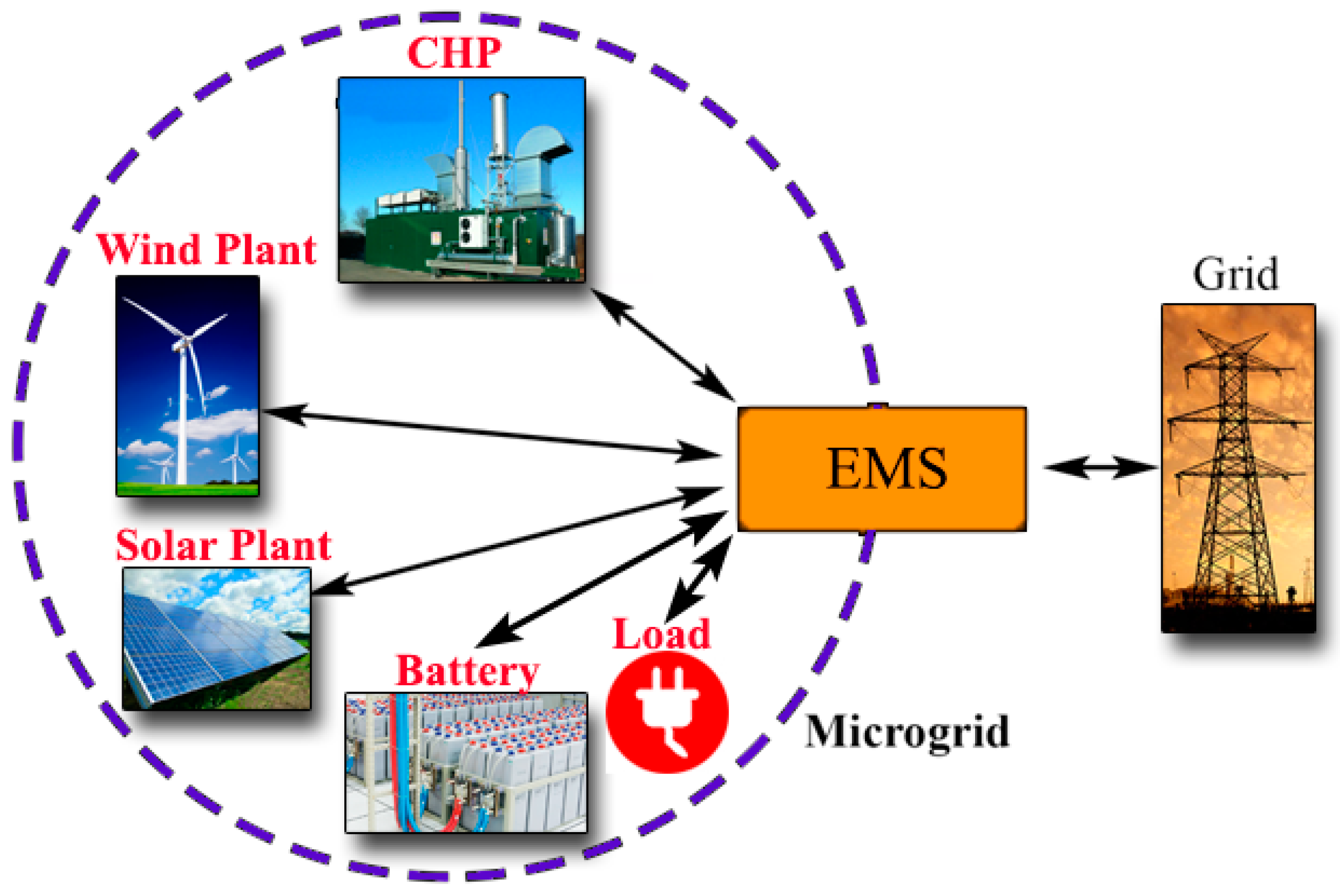
In this paper, a microgrid with a certain number of sources is considered, consisting of wind energy plants, solar PV plants, CHP, storage batteries and utility, as well as an EMS responsible for coordination of all components of the microgrid (Figure 1). The microgrid can be operated in grid-connected mode or disconnected (islanded) mode.
3. Efficient Energy Management System (EEMS)
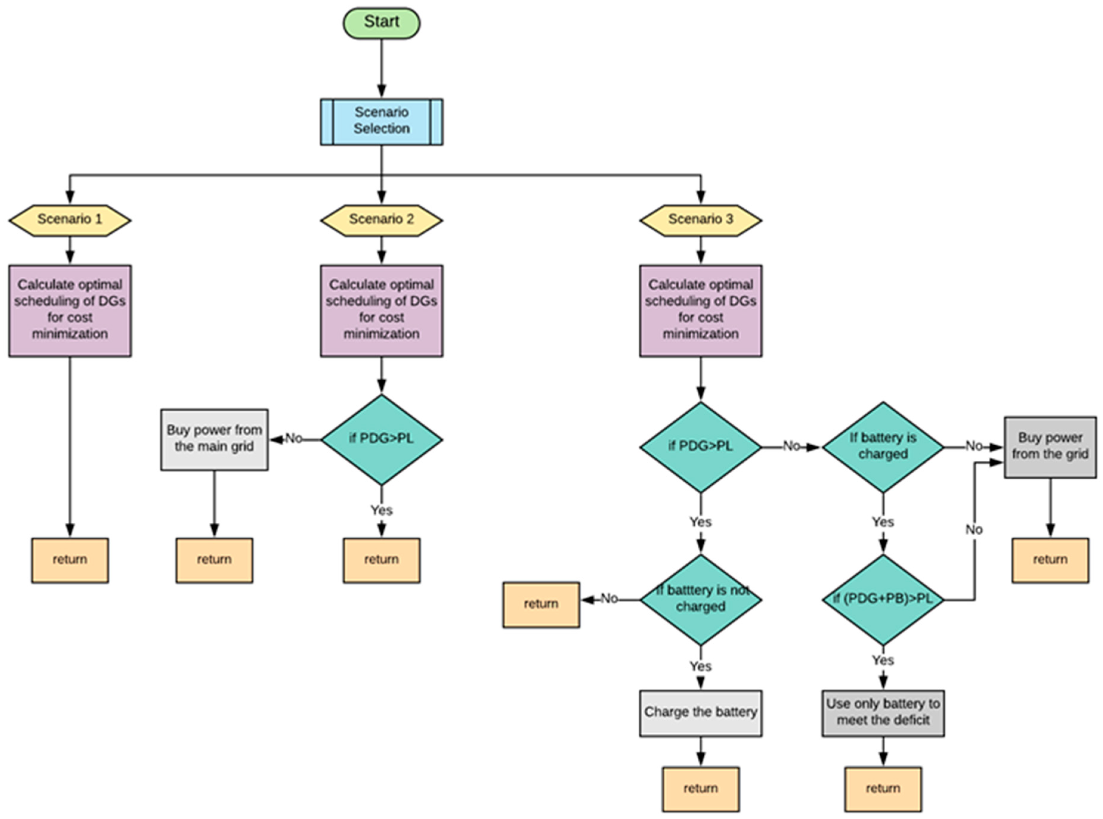
An EMS is required to coordinate the energy share among different sources of the microgrid based on the selected scenario. The word “efficient,” added to the EMS, demonstrates the proposed work uses EMVPA to make EMS operations more efficient in terms of running costs. The energy management strategy used in this study is represented by the flowchart given in Figure 2, which allows an operator to manage the microgrid using one scenario from the three defined scenarios. For all three scenarios, the main sources of energy are renewable sources. It is worth mentioning that, although three scenarios are investigated in this paper, more scenarios can be added to the EEMS. All proposed scenarios are described in the following subsections.
3.1. Scenario 1
All DGs can only be operated within their respective minimum and maximum limits. Moreover, there is no power that can be transferred from the utility or the main grid. Thus, the microgrid operates in islanded mode.
3.2. Scenario 2
All DGs can work within their limits and the microgrid can buy limited power from the utility only when DGs cannot supply the requested load.
3.3. Scenario 3
The microgrid has the facility of storage batteries and all DGs can work within their limits. The microgrid can buy limited power from the utility only when DGs and battery cannot supply the requested load. As shown in Figure 2, it is pertinent that if the generated power from DGs is greater than the load, the surplus energy is used to charge the battery bank. In the case where the battery bank is fully charged, no extra power will be generated from the DGs. On the other hand, if the power generated by DGs is less than the requested load, the deficit of power is provided by the battery bank. If DGs and the battery bank cannot supply the load, the deficit of power is bought from the main grid.
4. Optimization Problem
As aforesaid, the role of the EMS is to optimally schedule the different sources of the microgrid based on the selected scenario for each hour in order to minimize the operating cost of the microgrid under some constraints. This can be formulated mathematically as an optimization problem which is described in the following subsections.
4.1. Objective Function
The objective function of the considered optimization problem can be approximated by a quadratic nonlinear function as follows [39]:
where, denotes the number of DG units under consideration, and represent the cost in $ and power generated in MW on an hourly basis, respectively. DG technology and fuel cost are incorporated in coefficients , , and , where , specifically, is used to introduce DG related nonlinearity.
4.2. Design Variables
For this optimization problem, power generated by each DG is taken as a design variable. A solution is initially proposed in a vector form containing all design variables and given to the optimizer to optimize the solution in upcoming iterations and find a vector that contains the optimally distributed power output from each generator. A solution vector x, for n wind energy plants, m PV plants and k CHP, is given in the following expression:
where , , and represent the power from wind energy plants, solar PV plants and CHP, respectively.
4.3. Constraints
4.3.1. Power Balance
The power produced by the EEMS must be equal to the requested load at any instant. This can be represented by the following equation:
where is the total power required by the load at instant (t), is the power of storage batteries, and is the power from the grid at instant (t). It is worth to mention that, depend on the selected scenario. For example, for Scenario 1, there is no storage device used and the microgrid is not allowed to buy power from the main grid. For Scenario 2, there is no battery; however, when the DGs cannot supply the requested load at a given time the deficit of power is bought from the grid. Finally, for Scenario 3, there are batteries (that can charge and discharge) and if there is deficit in accumulative power of DGs and battery, the power needed will be provided by the main grid.
4.3.2. Power Limits
Each DG source is limited by a maximum value and a minimum value that can vary from one instant to another. This constraint can be expressed as follows:
where is the minimum value of power of ith DG at instant (t) and is the maximum value of power of ith DG at instant (t).
4.3.3. Battery Limits
The batteries are considered in this work as a secondary source of power. They can charge and discharge within a given range. Therefore, we can write the following constraint:
where is the minimum discharging value allowed for the batteries at time (t) and is the maximum charging capacity of the batteries.
5. Optimization Algorithms
To solve the considered optimization problem, an enhanced version of the MVPA is developed. This transforms the EMS system into a more efficient one; i.e., EEMS. In the following two sections, the classical version of the MVPA and the enhanced version will be explained. It is worth explaining here that using an enhanced version of the MVPA, which is a modern metaheuristic, instead of any other classical method is motivated by the advantages of modern metaheuristics over classical methods. Among these advantages is their ability to adapt to any problem with no/or few modifications, which allows them to be easily applied to different scenarios.
5.1. Most Valuable Player Algorithm
The MVPA is a new metaheuristic optimization algorithm developed by Bouchekara [40], inspired by sports events. The main step in the MVPA is a population of players that compete individually to win the Most Valuable Player (MVP) trophy and collectively to win the championship. One important feature of the MVPA is that it has no internal parameter to tune. In [41], a comparative study was carried out between metaheuristic algorithms inspired by sports events including the MVPA. The MVPA has been ranked first for unimodal problems and equally ranked first with two other algorithms for multimodal problems. In reference [42] the MVPA was used for circular antenna arrays optimization to maximize sidelobe levels reduction.
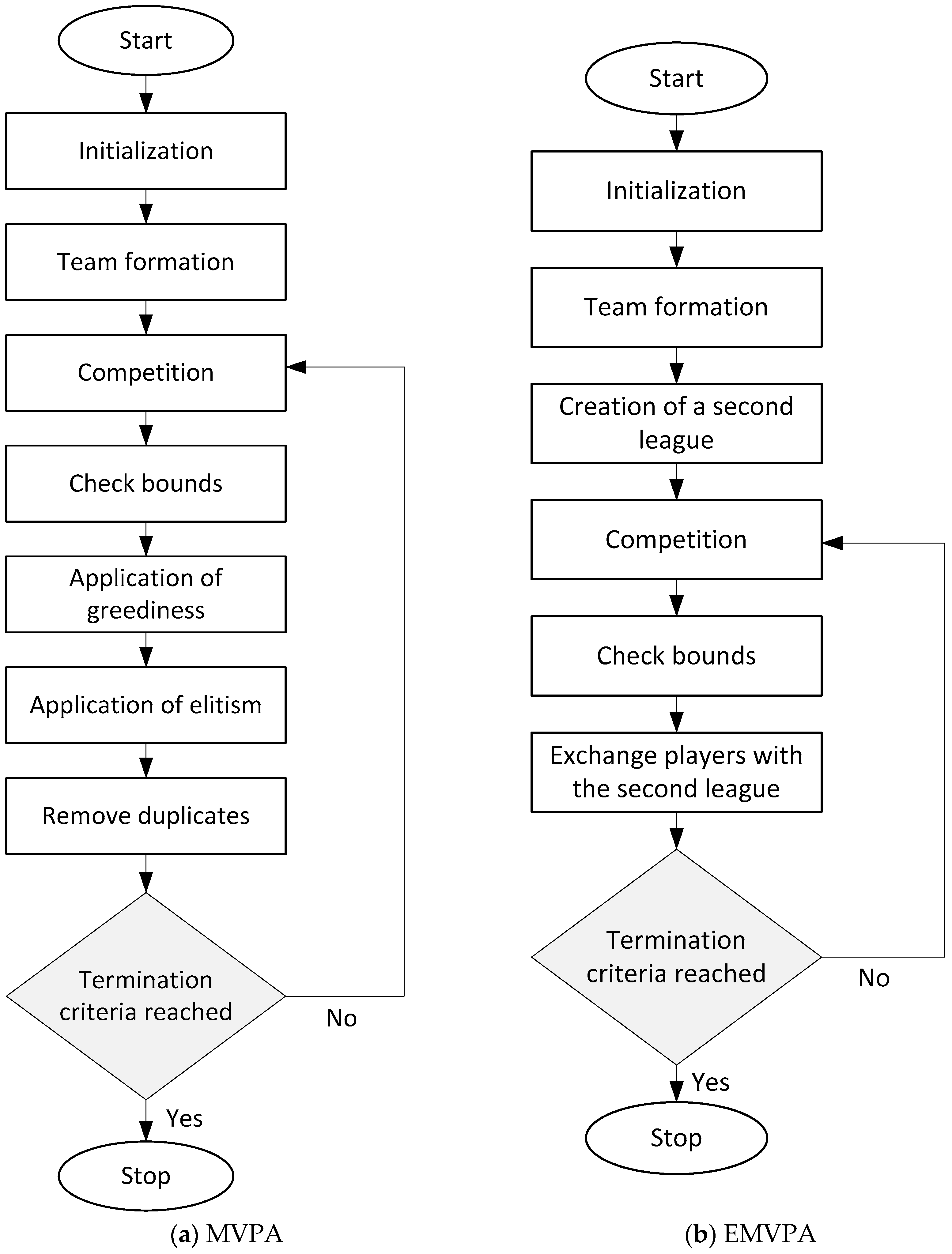
The flowchart of the MVPA is shown in Figure 3a. The inputs needed by the MVPA are:
- The objective function (noted as ObjFunction) which can be a mathematical explicit function or a more complicated one;
- The dimension of the problem (noted as ProblemSize) which represents the number of design variables of the treated problem;
- The number of players which is equivalent to the population size in other population-based optimization algorithms (noted as PlayersSize);
- The number of teams in the league noted as (TeamsSize); and
- The maximum number of fixtures (noted as MaxNFix) which is equivalent to the maximum number of iterations in other optimization algorithms.
The main output of the MVPA is the best solution obtained for the treated problem i.e., the MVP. However, the other outputs can easily be obtained, for example, the value of the best objective function obtained or the evaluation of this last value during the optimization process.
After reading the inputs, the MVPA starts with the initialization step as shown in Figure 3a. In this first step the players (i.e., solutions) are spread out randomly within the search space. In the second step, the players are regrouped to form TeamsSize teams followed by the most important step for the MVPA, the competition step.
The pseudocode of the competition step is given below:
| for i = 1: TeamsSize | ||
| Teams selection | Select the team number i from the league’s teams | |
| Randomly select another team j from the league’s teams where j ≠ i | ||
| Individual competition | ||
| Collective competition | if against | |
| else | ||
| end if | ||
| end for | ||
The competition step, as detailed in the pseudocode given above, starts with the selection of the first team (all teams are selected one after another as for the first team) and the opponent team which is selected randomly from the poll of teams where j ≠ i. In the individual competition phase, players compete and try individually to become their teams’ franchise players (the best player of their teams) and then to win the MVP trophy i.e., to become the league’s best player. In the collective competition phase, plays against and the players of are updated based on the results of the game. Teams aim to win the championship.
After the competition step, the players are checked and if any player is outside the search space, it is brought back to the crossed bound. This step is called check bounds in the flowchart of Figure 3a. Then, the objective function values of the players are compared to their initial values. If a player improves in the competition step, he is kept, otherwise the initial player is kept. This is called the greediness step in the flowchart of Figure 3a. After that, the last two steps aim to apply elitism and then remove duplicate players, respectively. Finally, if a predefined stopping criterion (or more generally a set of predefined criteria) is met, the process stops otherwise returns to Step 3 and iterates again following the same steps.
5.2. Enhanced Most Valuable Player Algorithm
The flowchart of the EMVPA is shown in Figure 3b. The EMVPA has the same structure as the MVPA, however, for the EMVPA a second league is created and after each iteration the best players of this league are traded to teams in the first league while the worst players are moved to the second league. As can be seen from Figure 3b, the EMVPA starts with the initialization step followed by the team formation step described above. After that, a second league (smaller than the main league) is created. Then, once the competition and check-bound steps are finished, players are exchanged between the two leagues. In this step the worst players of the main league are moved to the second league while the best players of the second league are moved to the first. Finally, the algorithm iterates Steps 4 to 6 until the desired number of iterations is reached. It is worth mentioning that, steps such as the ‘application of greediness’, ‘application of elitism’ and ‘remove duplicates’ are removed in the enhanced version of the MVPA.
6. Results and Discussion
The performance of the EEMS based on the proposed EMVPA is tested using two different microgrid systems. The obtained results are then compared with the performance of EMS using the MVPA, PSO, GA, black hole (BH) algorithm, artificial bee colony (ABC), and electromagnetism-like mechanism (EM) algorithm in order to assess the performance of the proposed EEMS. In the simulation, each algorithm is run 30 times, and the best results of each algorithm are reported. All algorithms (except MVPA and EMVPA) are initialized with a population size of 50. For MVPA and EMVPA, PlayersSize = 100 and TeamsSize = 20. Moreover, the maximum number of iterations is set at 1000 for all algorithms and for all cases.
It must be noted that the developed codes and programs are run using MATLAB software on Core i7 @ 2.50 GHz, 8 GB RAM machine.
6.1. Microgrid #1
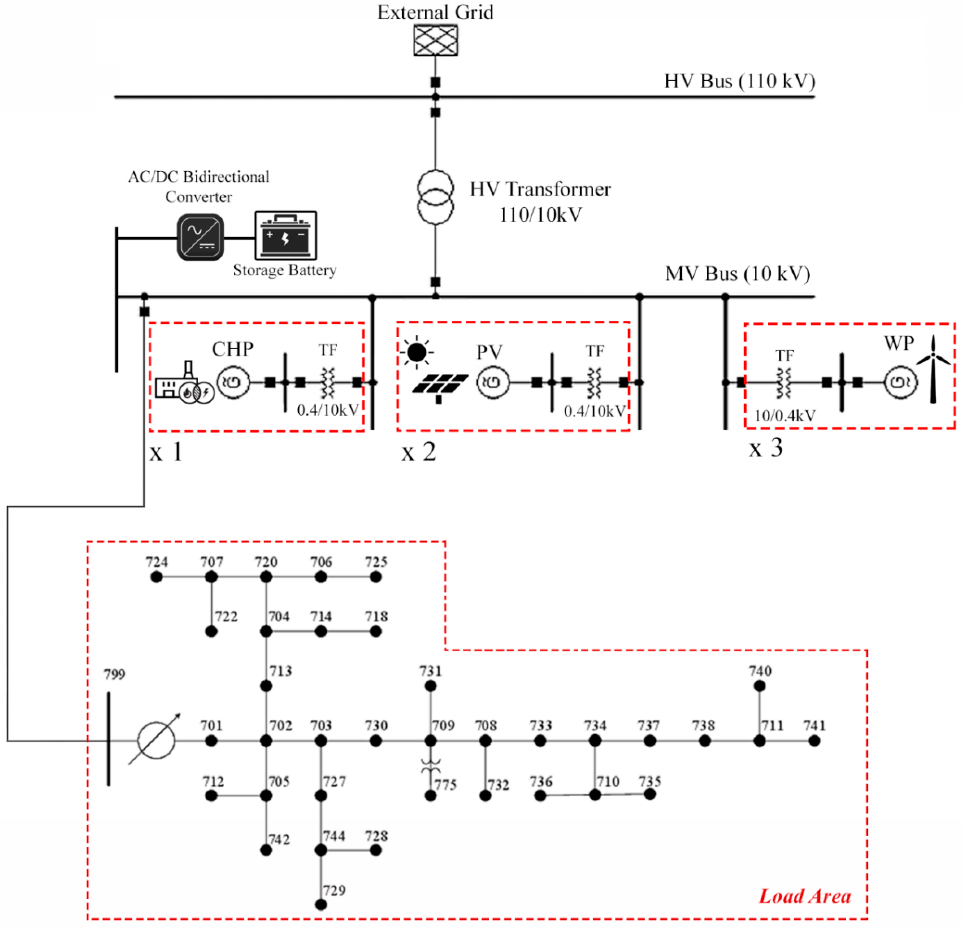
The first microgrid investigated in this paper is shown in Figure 4. This microgrid consists of a load area represented by the IEEE 37-bus test system, five DGs, a CHP, and a storage battery source.
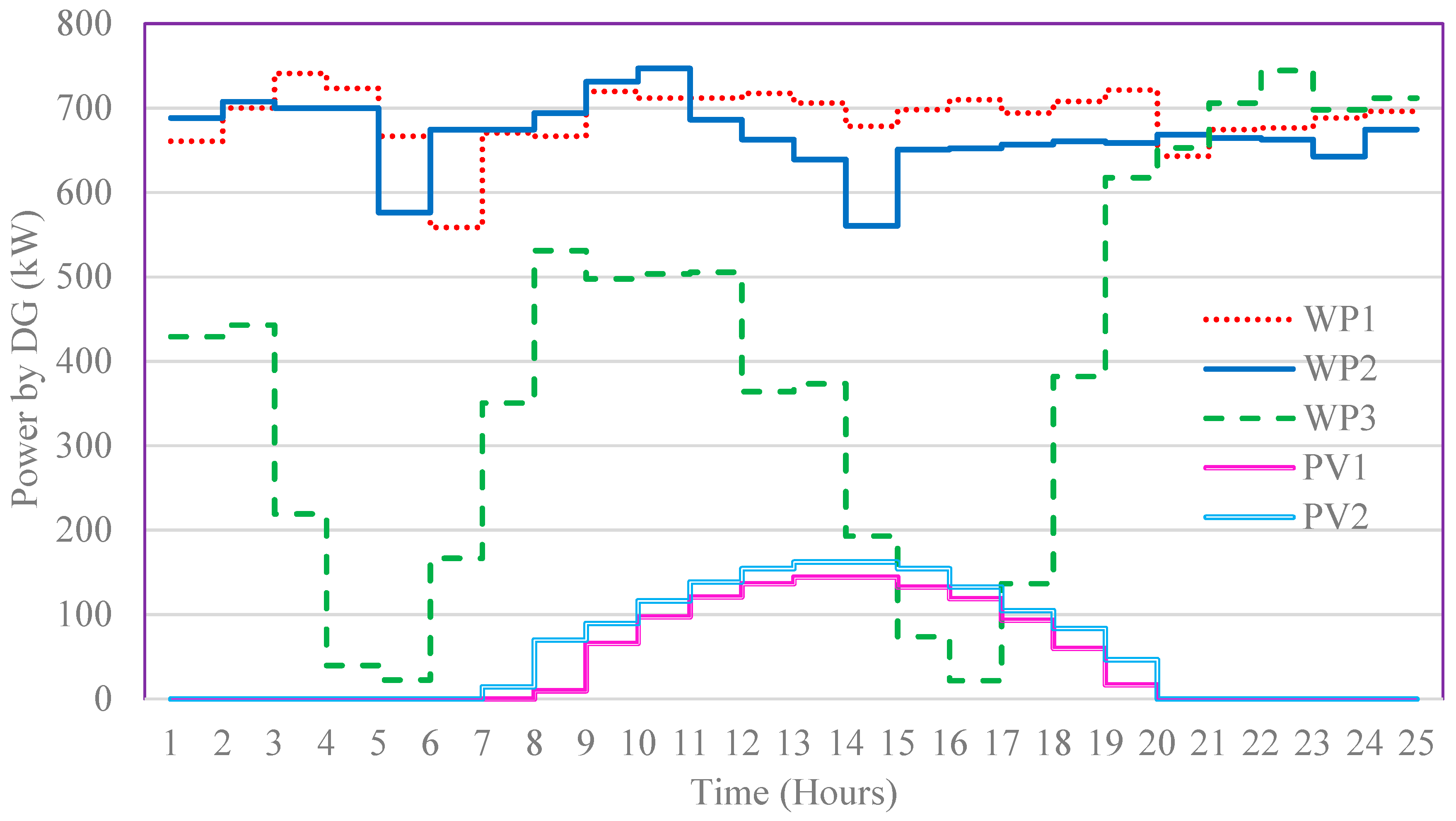
The individual maximum capacities of CHP, each PV, and wind energy plant are 1000 kW, 250 kW, and 750 kW, respectively. The CHP can run at full capacity for the entire day, i.e., it can provide 1000 kW at any time, however, due to the intermittency of renewable energy sources, the power output from wind and PV plants is irregular. The power availability for each DG per hour in a running day is shown in Figure 5 [4]. The battery has a storage capacity of 300 kWh.
The load demand follows an hourly trend, given in Table 1 [4]. It can be noted that the load peaks between hour 18 and hour 23. The electricity price (from the main grid) is given in Table 1. Furthermore, the coefficients of the cost function of different DGs are tabulated in Table 2 [4]. These coefficients are based on the technology used for each DG.
6.1.1. Case 1 (Scenario 1)
It is assumed that renewable energy sources will never run out and, therefore, the microgrid will never need to rely on battery storage, virtual power plants, or the utility grid. The optimization results for the first scenario are presented in Table 3. In this table, the first column represents the hour of the day, the second set of columns represent the power of each unit, the third set of columns represents the cost needed to generate the required power for each unit, and the last column represents the total cost of generating the required load at each hour.
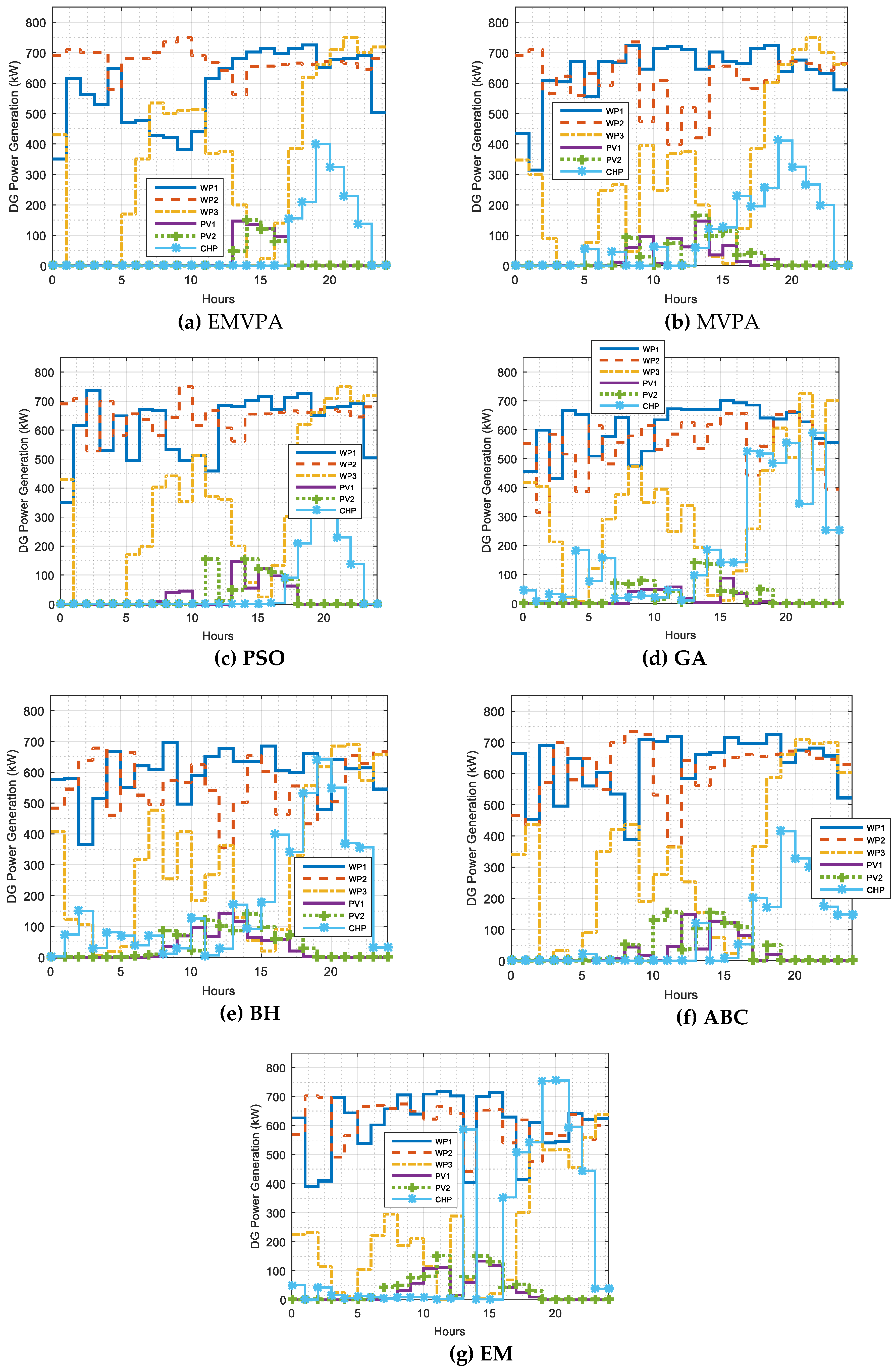
Figure 6 shows the optimal energy management among all DGs as optimized by the EMVPA, MVPA, PSO, GA, BH, ABC, and EM, over the course of 24 hours. Basically, these graphs indicate the power produced by each DG at a given hour. It can be noted that for all algorithms, the sum of power produced by all DGs equals the load demand, maintaining the load demand balance.
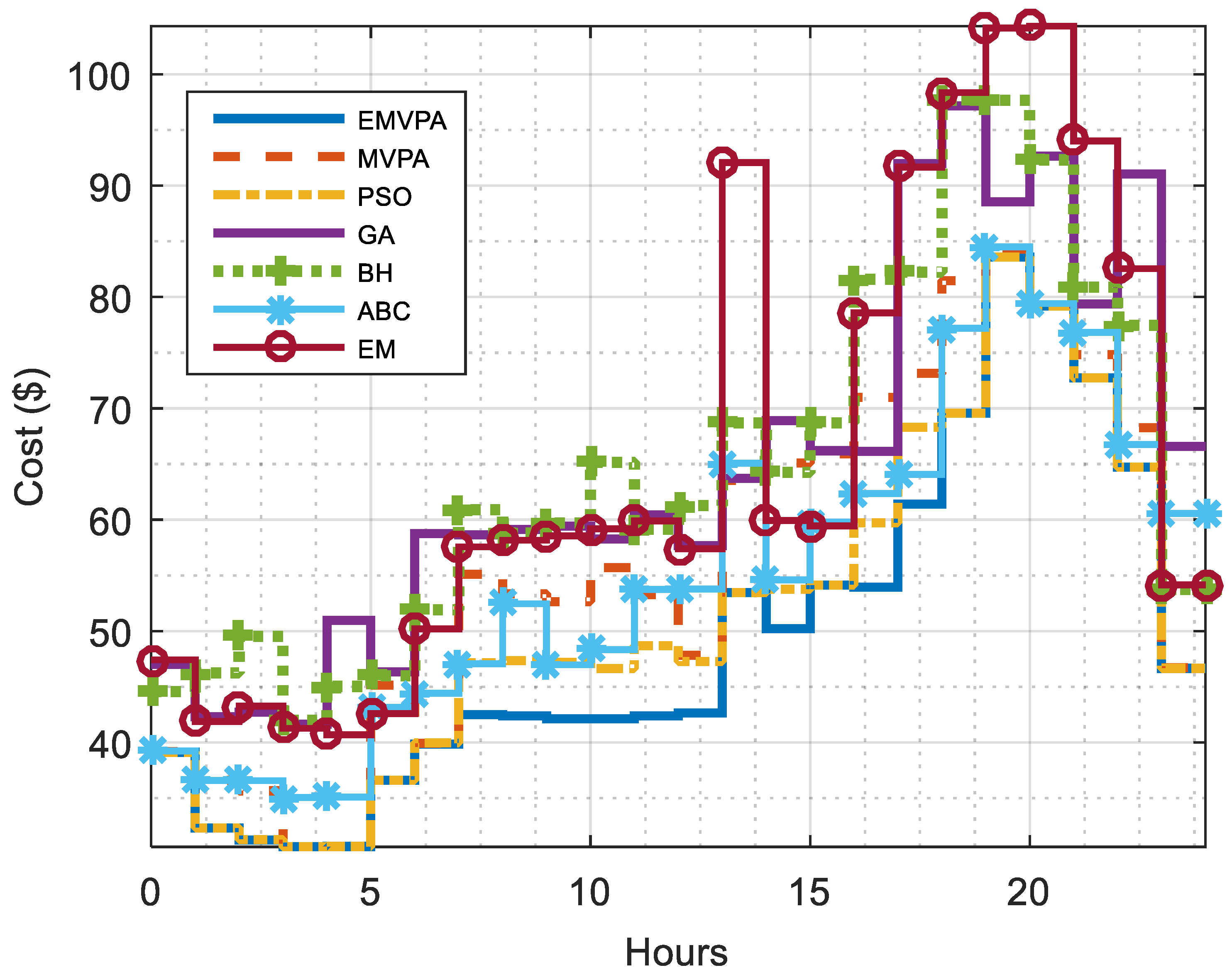
The total costs per hour obtained by the EMS using different algorithms are given in detail in Table 4 which are also illustrated in Figure 7. The last row of this table gives the total cost for 24 hours. Total cost obtained using the EMVPA is $1184.18, which is the lowest among the tested algorithms. The second-best algorithm for Case 1 is PSO which gives a total cost of $1230.709, while the third algorithm, the ABC, gives a total cost of $1323.594. It can also be seen from Table 4 that the EMVPA achieved better results at any hour, which gives the minimum cost of EEMS, being the best power system scheduling solution at any instant.
6.1.2. Case 2 (Scenario 2)
The load given in Table 1 is assumed to be increased by 10% and the CHP is not operated. Table 5 provides the optimization results for this case. It can be seen that the EEMS buys power from the main grid only when there is a deficit of power (in hour 5 and hour 6, for instance). In such cases all DGs must run at their maximum capacity.
The results obtained using the EMVPA are compared with the results optimized by the other algorithms as shown in Table 6 and Figure 8. The total cost obtained by the EEMS using the EMVPA is the lowest (equally with PSO) among the tested algorithms at $1132.384. The initial version of the MVPA ranks third at an operating cost of $1137.679.
6.1.3. Case 3 (Scenario 3)
The operating strategy of this case is identical to that of the case using Scenario 2 in the previous subsection. However, this case differs from Case 2 in that the storage capability is available. The optimization of the microgrid under Scenario 3 was completed and the results are provided in Table 7. It can be noted that when there is a surplus of power from the DGs, the battery is charged on an hourly basis, as for hour 1 and hour 2. However, the battery cannot exceed its maximum charging capacity. For this reason, the battery is no longer being charged in hour 3 and hour 4. Moreover, when there is a deficit of power from the DGs sources, in hour 6 for example, the battery is discharged and used as a second source of power after DGs. However, when the DGs and battery together cannot supply the load, the power is bought from the grid; hours 19 and 20 serve as an example for this situation.
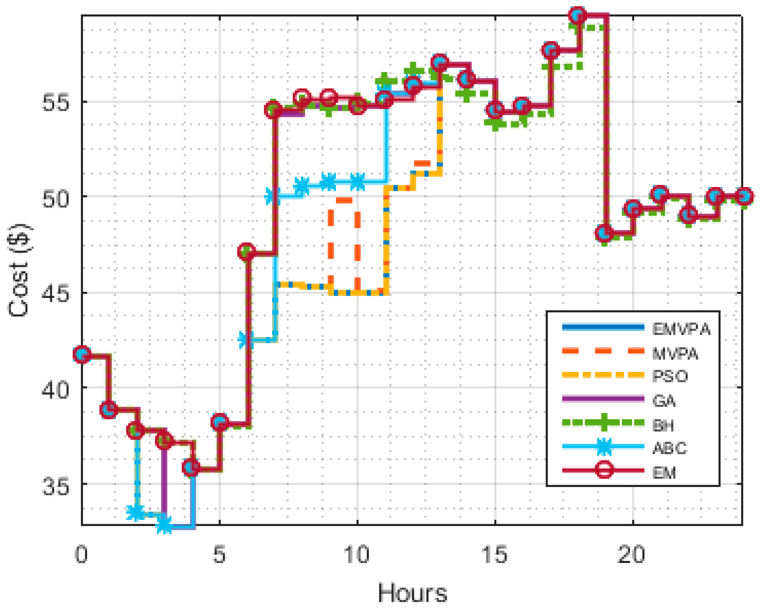
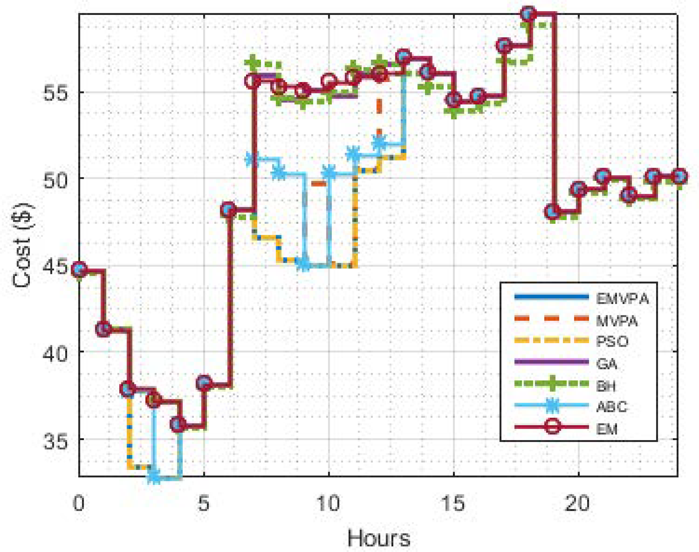
The total costs per hour obtained by the EMS using the investigated algorithms are tabulated in Table 8 and sketched in Figure 9. The total cost obtained using the EMVPA is $1144.694, which is the lowest cost among the algorithms. The second-best algorithm for Case 3 is the PSO which gives a total cost of $1144.695, whilst the third algorithm is the MVPA, which has a total cost of $1154.013. It can also be seen from Table 8 that the EMVPA achieved better results than the tested algorithms at any hour.
6.2. Microgrid #2
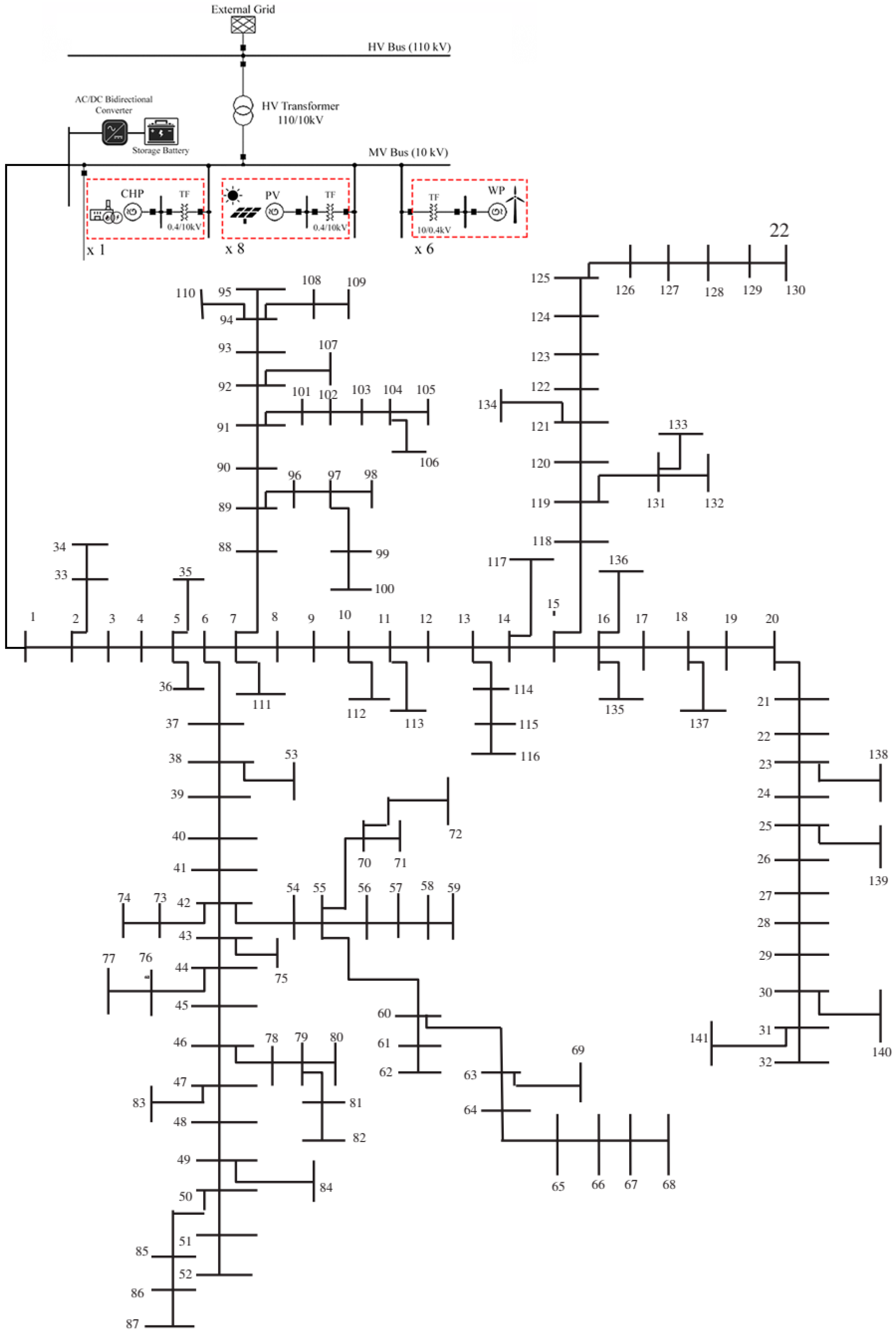
To assess the performance of the proposed EEMS on a large-scale test system, a second microgrid is considered as shown in Figure 10. The microgrid consists of a load area represented by the 141-bus test system with 14 DGs, a CHP, and a storage battery source. The data used for the second system is given in Table 9 and Table 10.
Case 4 (Scenario 3)
This case simulates the operating strategy of Scenario 3 in Figure 2, as analyzed in Case 3 of microgrid #1. The optimization results obtained using the EMVPA are provided in detail in Table 11 and Table 12. It can be seen from Table 11 that when the capacity of the DGs is greater than the load, the battery is charged in hour 1 and hour 18. The grid is needed only when the DGs and battery cannot supply the requested power as given in hours 15, 16, and 17.
The total costs obtained by the EMS using the investigated algorithms are shown in Table 13. A simple comparison between the different algorithms shows that the EMVPA has the lowest total cost of $ 3883.633 followed by the PSO and the ABC, which give $3940.981 and $3989.233, respectively. This result again demonstrates the superiority of the EEMS based on the EMVPA compared to the other algorithms.
6.3. Daily Cost Reduction Analysis
Table 14 presents the percentage of daily cost reduction obtained using EMVPA compared with the remaining algorithms. It can be observed from this table that the EMVPA presents high-cost reductions for Case 1 and Case 4 and moderate cost reductions for Case 2 and Case 3. The highest cost reduction percentage is obtained for Case 1 compared to the EM. For Case 2 and Case 3, the results of the EMVPA and the PSO are almost identical. These results confirm the superiority of the EMVPA compared with the other algorithms at optimizing the energy management of microgrids.
Moreover, it is worth mentioning that, for microgrid #1 the calculation speed of the EMVPA is around 12 s per hour while for the calculation speed for microgrid #2 is around 23 s per hour.
7. Conclusions
In this paper, an EEMS based on an enhanced version of the most valuable player algorithm is proposed and developed to optimize the operation of a microgrid by minimizing the operating cost. The EEMS aims to schedule different sources of energy based on a selected scenario. In the first scenario, the power generated from DGs is always greater than the requested load. In the second scenario, the EEMS can buy energy from the grid only when the DGs cannot supply the requested load. In the last scenario, a battery storage is added to the microgrid, which is the second source of power after DGs, while the main grid is the last option. It is obvious that more scenarios can be added to the EEMS in the future.
In comparison to other optimization algorithms, the proposed EEMS using the EMVPA achieves better results and can determine the optimal scheduling of different DGs, battery storage, and the power needed from the grid based on the selected scenario. Moreover, four cases for two different microgrids were investigated. For Case 1, the daily cost reduction varies from 3.781% for the PSO (the second-best method after the EMVPA) to 24.925% for the EM (the worst method for this case). Likewise, for Case 2, it varies from 0% for the PSO to 5.126% for the EM. For Case 3, it varies from 0% for the PSO to 4.872% for the EM. Finally, for Case 4, the daily cost reduction varies from 1.455% for the PSO to 10.039% for the EM. Furthermore, it is found that the EEMS using the proposed EMVPA provides the most cost-effective solution for each hour ensuring its efficacy and robustness. Since energy markets are moving towards real-time pricing, such a modified approach is highly desirable to effectively address power-sharing problems.
The optimization results using the proposed method is expected to give an optimal energy management system strategy, which will assist energy practitioners in managing generation units and energy storage devices in renewable energy based microgrids. Furthermore, the results of this study may have implications for future implementation of microgrid projects and renewable energy resources development in general.
Further research is recommended in the following areas: Additional scenarios can be investigated and the influence of the efficiency of forecasting models can be assessed, while unbalanced microgrid systems can also be investigated. Also, uncertainty modeling of load demands and renewable generation can be included in these models.
Author Contributions
M.A.M.R. has contributed on conceptualization, article writing and review; H.R.E.H.B. have contributed on simulation and article writing; A.S.A. have contributed on supervision and article writing.
Funding
This project was funded by the Deanship of Scientific Research (DSR) at King Abdulaziz University, Jeddah, under grant no. (G/452/135/1439). The authors, therefore, acknowledge with thanks DSR for technical and financial support.
Conflicts of Interest
The authors declare no conflicts of interest.
Nomenclature
| ABC | Artificial bee colony |
| AFSA | Artificial fish swarm algorithm |
| BB–BC | Big bang-big crunch |
| BH | Black hole algorithm |
| Cost in $ | |
| CHP | Combined heat and power |
| DE | Differential evolution |
| DG | Distributed generation |
| EM | Electromagnetism-like mechanism |
| EMS | Energy management system |
| EMVPA | Enhanced most valuable player algorithm |
| GA | Genetic algorithm |
| HS | Harmony search |
| MaxNFix | Maximum number of fixtures which is equivalent to the maximum number of iterations |
| MDP | Markov decision process |
| MILP | Mixed integer linear programming |
| MVPA | Most valuable player algorithm |
| NSGA | Non-dominated sorting genetic algorithm |
| ObjFunction | Objective function |
| Power generated in MW | |
| Power of storage batteries at instant (t) | |
| Maximum charging capacity of the batteries at time (t) | |
| Minimum discharging value allowed for the batteries at time (t) | |
| Power from the grid at instant (t) | |
| Maximum value of power of ith DG at instant (t) | |
| Minimum value of power of ith DG at instant (t) | |
| Total power required by the load at instant (t) | |
| PlayersSize | Number of players which is equivalent to the population size |
| ProblemSize | Dimension of the problem |
| PSO | Particle swarm optimization |
| PV | Photovoltaic |
| TeamsSize | Number of teams in the league |
| WCA | Water cycle algorithm |
| , , and | Cost coefficients |
References
- Kumar, K.P.; Saravanan, B.; Swarup, K.S. Optimization of Renewable Energy Sources in a Microgrid Using Artificial Fish Swarm Algorithm. Energy Procedia 2016, 90, 107–113. [Google Scholar] [CrossRef]
- Zhang, J.; Wu, Y.; Guo, Y.; Wang, B.; Wang, H.; Liu, H. A hybrid harmony search algorithm with differential evolution for day-ahead scheduling problem of a microgrid with consideration of power flow constraints. Appl. Energy 2016, 183, 791–804. [Google Scholar] [CrossRef]
- Maulik, A.; Das, D. Optimal operation of microgrid using four different optimization techniques. Sustain. Energy Technol. Assess. 2017, 21, 100–120. [Google Scholar] [CrossRef]
- Crisostomi, E.; Liu, M.; Raugi, M.; Shorten, R. Plug-and-play distributed algorithms for optimized power generation in a microgrid. IEEE Trans. Smart Grid 2014, 5, 2145–2154. [Google Scholar] [CrossRef]
- Amrollahi, M.H.; Bathaee, S.M.T. Techno-economic optimization of hybrid photovoltaic/wind generation together with energy storage system in a stand-alone micro-grid subjected to demand response. Appl. Energy 2017, 202, 66–77. [Google Scholar] [CrossRef]
- Li, B.; Roche, R.; Miraoui, A. Microgrid sizing with combined evolutionary algorithm and MILP unit commitment. Appl. Energy 2017, 188, 547–562. [Google Scholar] [CrossRef] [Green Version]
- Azaza, M.; Wallin, F. Multi objective particle swarm optimization of hybrid micro-grid system: A case study in Sweden. Energy 2017, 123, 108–118. [Google Scholar] [CrossRef]
- Santiago, D.M.L.; Bravo, E.P.C. Multi-objective optimal power management in microgrids: A comparative study. In Proceedings of the 2015 IEEE PES Innovative Smart Grid Technologies Latin America (ISGT LATAM), Montevideo, Uruguay, 5–7 October 2015. [Google Scholar]
- Wasilewski, J. Optimisation of multicarrier microgrid layout using selected metaheuristics. Int. J. Electr. Power Energy Syst. 2018, 99, 246–260. [Google Scholar] [CrossRef]
- Luna-Rubio, R.; Trejo-Perea, M.; Vargas-V_azquez, D.; Ríos-Moreno, G.J. Optimal sizing of renewable hybrids energy systems: A review of methodologies. Sol. Energy 2012, 86, 1077–1088. [Google Scholar] [CrossRef]
- Schutte, J.F.; Koh, B.I.; Reibolt, J.A.; Haftka, R.T.; George, A.D.; Fregly, B.J. Evaluation of a particle swarm algorithm for biomechanical optimization. J. Biomech. Eng. 2005, 127, 465–474. [Google Scholar] [CrossRef]
- Harmouch, F.Z.; Krami, N.; Hmina, N. A multiagent based decentralized energy management system for power exchange minimization in microgrid cluster. Sustain. Cities Soc. 2018, 40, 416–427. [Google Scholar] [CrossRef]
- Zia, M.F.; Elbouchikhi, E.; Benbouzid, M. Microgrids energy management systems: A critical review on methods, solutions, and prospects. Appl. Energy 2018, 222, 1033–1055. [Google Scholar] [CrossRef]
- Wang, S.; Su, L.; Zhang, J. MPI based PSO algorithm for the optimization problem in micro-grid energy management system. In Proceedings of the 2017 Chinese Automation Congress (CAC), Jinan, China, 20–22 October 2017. [Google Scholar]
- Deihimi, A.; Keshavarz Zahed, B.; Iravani, R. An interactive operation management of a micro-grid with multiple distributed generations using multi-objective uniform water cycle algorithm. Energy 2016, 106, 482–509. [Google Scholar] [CrossRef]
- Elsied, M.; Oukaour, A.; Gualous, H.; Lo Brutto, O.A. Optimal economic and environment operation of micro-grid power systems. Energy Convers. Manag. 2016, 122, 182–194. [Google Scholar] [CrossRef]
- Li, P.; Xu, D. Optimal operation of microgrid based on improved binary particle swarm optimization algorithm with double-structure coding. In Proceedings of the 2014 International Conference on Power System Technology, Chengdu, China, 20–22 October 2014. [Google Scholar]
- Litchy, J.; Nehrir, M.H. Real-time energy management of an islanded microgrid using multi-objective Particle Swarm Optimization. In Proceedings of the 2014 IEEE PES General Meeting Conference & Exposition, National Harbor, MD, USA, 27–31 July 2014. [Google Scholar]
- Kitamura Mori, K.; Shindo SIzui, Y.; Ozaki, Y. Multiobjective energy management system using modified MOPSOS. In Proceedings of the 2005 IEEE International Conference on Systems, Man and Cybernetics, Waikoloa, HI, USA, 12 October 2005. [Google Scholar]
- Sedighizadeh, M.; Esmaili, M.; Eisapour-Moarref, A. Voltage and frequency regulation in autonomous microgrids using Hybrid Big Bang-Big Crunch algorithm. Appl. Soft Comput. 2017, 52, 176–189. [Google Scholar] [CrossRef]
- Abedini, M.; Abedini, M. Optimizing energy management and control of distributed generation resources in islanded microgrids. Util. Policy Vol. 2017, 48, 32–40. [Google Scholar] [CrossRef]
- De Santis, E.; Rizzi, A.; Sadeghia, A. Hierarchical genetic optimization of a fuzzy logic system for energy flows management in microgrids. Appl. Soft Comput. 2017, 60, 135–149. [Google Scholar] [CrossRef] [Green Version]
- Zhang, Y.; Meng, F.; Wang, R.; Zhu, W.; Zeng, X. A stochastic MPC based approach to integrated energy management in microgrids. Sustain. Cities Soc. 2018, 41, 349–362. [Google Scholar] [CrossRef]
- Phurailatpa, C.; Rajpurohit, B.S.; Wang, L. Planning and optimization of autonomous DC microgrids for rural and urban applications in India. Renew. Sustain. Energy Rev. 2018, 82, 1194–1204. [Google Scholar]
- Jiang, F.; Xie, H.; Ellen, O. Hybrid energy system with optimized storage for improvement of sustainability in a small town. Sustainability 2018, 10, 2034. [Google Scholar] [CrossRef]
- Alvarez, E.; Campos, A.M.; Arboleya, P.; Gutierrez, A.J. Microgrid management with a quick response optimization algorithm for active power dispatch. Int. J. Electr. Power Energy Syst. 2012, 43, 465–473. [Google Scholar] [CrossRef]
- Ghasemi, A.; Enayatzare, M. Optimal energy management of a renewable-based isolated microgrid with pumped-storage unit and demand response. Renew. Energy 2018, 123, 460–474. [Google Scholar] [CrossRef]
- Kim, H.; Bae, J.; Baek, S.; Nam, D.; Cho, H.; Chang, H. Comparative analysis between the government micro-grid plan and computer simulation results based on real data: The practical case for a South Korean Island. Sustainability 2017, 9, 197. [Google Scholar] [CrossRef]
- Yousefi, H.; Ghodusinejad, M.H. Feasibility study of a hybrid energy system for emergency off-grid operating conditions. Majlesi J. Electr. Eng. 2017, 11, 7–14. [Google Scholar]
- Sardou, I.G.; Zare, M.; Farsani, E.A. Robust energy management of a microgrid with photovoltaic inverters in VAR compensation mode. Int. J. Electr. Power Energy Syst. 2018, 98, 118–132. [Google Scholar] [CrossRef]
- Zhang, Y.; Gatsis, N.; Giannakis, G.B. Robust Energy Management for Microgrids With High-Penetration Renewables. IEEE Trans. Sustain. Energy 2013, 4, 944–953. [Google Scholar] [CrossRef]
- Su, W.; Wang, J.; Member, S.; Roh, J. Stochastic Energy Scheduling in Microgrids with Intermittent Renewable Energy Resources Stochastic Energy Scheduling in Microgrids With Intermittent Renewable Energy Resources. IEEE Trans. Smart Grid 2013, 5, 1876–1883. [Google Scholar] [CrossRef]
- Bruno, S.; Dellino, G.; La Scala, M.; Meloni, C. A Microforecasting Module for Energy Management in Residential and Tertiary Buildings. Energies 2019, 12, 1006. [Google Scholar] [CrossRef]
- Singh, S.; Singh, M.; Kaushik, S.C. Optimal power scheduling of renewable energy systems in microgrids using distributed energy storage system. IET Renew. Power Gener. 2016, 10, 1328–1339. [Google Scholar] [CrossRef]
- Lan, Y.; Guan, X.; Wu, J. Rollout strategies for real-time multi-energy scheduling in microgrid with storage system. IET Gener. Trans. Distrib. 2016, 10, 688–696. [Google Scholar] [CrossRef]
- Askarzadeh, A. A Memory-based Genetic Algorithm for Optimization of Power Generation in a Microgrid. IEEE Trans Sustain. Energy 2018, 9, 1081–1089. [Google Scholar] [CrossRef]
- Chen, C.; Lee, T.; Jan, R.; Lu, C. A novel direct search approach for combined heat and power dispatch. Int. J. Electr. Power Energy Syst. 2012, 43, 766–773. [Google Scholar] [CrossRef]
- Blake, S.T.; O’Sullivan, D.T.J. Optimization of Distributed Energy Resources in an Industrial Microgrid. Procedia CIRP 2018, 67, 104–109. [Google Scholar] [CrossRef]
- Silvente, J.; Papageorgiou, L.G. An MILP formulation for the optimal management of microgrids with task interruptions. Appl. Energy 2017, 206, 1131–1146. [Google Scholar] [CrossRef] [Green Version]
- Bouchekara, H.R.E.H. Most Valuable Player Algorithm: A novel optimization algorithm inspired from sport. Oper. Res. 2017, 1–57. [Google Scholar] [CrossRef]
- Alatas, B. Sports inspired computational intelligence algorithms for global optimization. Artif. Intell. Rev. 2017, 1–49. [Google Scholar] [CrossRef]
- Bouchekara, H.R.E.; Orlandi, A.; Al-Qdah, M.; de Paulis, F. Most Valuable Player Algorithm for Circular Antenna Arrays Optimization to Maximum Sidelobe Levels Reduction. IEEE Trans. Electromagn. Compat. 2018, 60, 1655–1661. [Google Scholar] [CrossRef]
- Khodr, H.M.; Olsina, F.G.; De Oliveira-De Jesus, P.M.; Yusta, J.M. Maximum savings approach for location and sizing of capacitors in distribution systems. Electr. Power Syst. Res. 2008, 78, 1192–1203. [Google Scholar] [CrossRef]
Figure 1.
Microgrid representation.

Figure 2.
Flowchart of the proposed EMS of the microgrid.

Figure 3.
Flowchart of the MVPA and the EMVPA.

Figure 4.
Schematic of power system with five DGs and IEEE 37-node test feeder.

Figure 5.
Hourly availability of power by intermittent DGs [4].
Figure 5.
Hourly availability of power by intermittent DGs [4].

Figure 6.
Optimal scheduling of DGs for Case 1 using tested algorithms.

Figure 7.
Total cost per hour obtained by the EMS using tested algorithms for Case 1.

Figure 8.
Total cost per hour obtained by the EMS using tested algorithms for Case 2.

Figure 9.
Total cost per hour obtained by the EMS using tested algorithms for Case 3.

Figure 10.
Schematic of power system with fourteen DGs and 141-node test feeder.


Table 1.
Load demand [4] and electricity price per hour.
Table 1.
Load demand [4] and electricity price per hour.
| Hour | Load (kW) | Electricity Price ($/kWh) |
|---|---|---|
| 1 | 1471 | 0.043 |
| 2 | 1325 | 0.035 |
| 3 | 1263 | 0.026 |
| 4 | 1229 | 0.022 |
| 5 | 1229 | 0.022 |
| 6 | 1321 | 0.038 |
| 7 | 1509 | 0.043 |
| 8 | 1663 | 0.07 |
| 9 | 1657 | 0.28 |
| 10 | 1643 | 0.744 |
| 11 | 1643 | 0.744 |
| 12 | 1652 | 0.744 |
| 13 | 1666 | 0.28 |
| 14 | 1639 | 0.744 |
| 15 | 1642 | 0.372 |
| 16 | 1640 | 0.363 |
| 17 | 1676 | 0.112 |
| 18 | 1920 | 0.077 |
| 19 | 2214 | 0.065 |
| 20 | 2382 | 0.079 |
| 21 | 2382 | 0.235 |
| 22 | 2327 | 0.1 |
| 23 | 2174 | 0.056 |
| 24 | 1903 | 0.048 |
Table 2.
Cost coefficients of DG [4].
Table 2.
Cost coefficients of DG [4].
| Plant | WP1 | WP2 | WP3 | PV1 | PV2 | CHP |
|---|---|---|---|---|---|---|
| α | 0.0027 | 0.0028 | 0.0026 | 0.0055 | 0.0055 | 0.0083 |
| β | 17.83 | 17.54 | 17.23 | 29.3 | 29.58 | 75.73 |
| γ | 4.46 | 4.45 | 4.44 | 4.45 | 4.46 | 5.21 |
Table 3.
Optimal energy management (powers and costs) obtained by the EEMS using EMVPA for Case 1.
| Hour | Power (kW) | Cost ($) | Total Cost ($) | ||||||||||
|---|---|---|---|---|---|---|---|---|---|---|---|---|---|
| WP1 | WP2 | WP3 | PV1 | PV2 | CHP | WP1 | WP2 | WP3 | PV1 | PV2 | CHP | ||
| 1 | 351 | 690 | 430 | 0 | 0 | 0 | 10.719 | 16.554 | 11.849 | 0 | 0 | 0 | 39.122 |
| 2 | 615 | 710 | 0 | 0 | 0 | 0 | 15.426 | 16.905 | 0 | 0 | 0 | 0 | 32.331 |
| 3 | 563 | 700 | 0 | 0 | 0 | 0 | 14.499 | 16.729 | 0 | 0 | 0 | 0 | 31.229 |
| 4 | 529 | 700 | 0 | 0 | 0 | 0 | 13.893 | 16.729 | 0 | 0 | 0 | 0 | 30.622 |
| 5 | 649 | 580 | 0 | 0 | 0 | 0 | 16.033 | 14.624 | 0 | 0 | 0 | 0 | 30.657 |
| 6 | 471 | 680 | 170 | 0 | 0 | 0 | 12.859 | 16.378 | 7.369 | 0 | 0 | 0 | 36.606 |
| 7 | 478 | 680 | 351 | 0 | 0 | 0 | 12.983 | 16.378 | 10.488 | 0 | 0 | 0 | 39.850 |
| 8 | 428 | 700 | 535 | 0 | 0 | 0 | 12.092 | 16.729 | 13.659 | 0 | 0 | 0 | 42.480 |
| 9 | 422 | 735 | 500 | 0 | 0 | 0 | 11.985 | 17.343 | 13.056 | 0 | 0 | 0 | 42.384 |
| 10 | 383 | 750 | 510 | 0 | 0 | 0 | 11.289 | 17.607 | 13.228 | 0 | 0 | 0 | 42.124 |
| 11 | 440 | 690 | 513 | 0 | 0 | 0 | 12.306 | 16.554 | 13.280 | 0 | 0 | 0 | 42.139 |
| 12 | 615 | 667 | 370 | 0 | 0 | 0 | 15.426 | 16.150 | 10.815 | 0 | 0 | 0 | 42.392 |
| 13 | 649 | 642 | 375 | 0 | 0 | 0 | 16.033 | 15.712 | 10.902 | 0 | 0 | 0 | 42.646 |
| 14 | 682 | 562 | 200 | 147 | 48 | 0 | 16.621 | 14.308 | 7.886 | 8.757 | 5.880 | 0 | 53.453 |
| 15 | 702 | 655 | 0 | 135 | 150 | 0 | 16.978 | 15.940 | 0 | 8.406 | 8.897 | 0 | 50.221 |
| 16 | 715 | 656 | 24.950 | 122 | 122.050 | 0 | 17.210 | 15.957 | 4.870 | 8.025 | 8.070 | 0 | 54.132 |
| 17 | 697 | 661 | 140 | 97 | 81 | 0 | 16.889 | 16.045 | 6.852 | 7.292 | 6.856 | 0 | 53.934 |
| 18 | 713 | 666 | 385 | 0 | 0 | 156 | 17.174 | 16.133 | 11.074 | 0 | 0 | 17.024 | 61.405 |
| 19 | 725 | 660 | 620 | 0 | 0 | 209 | 17.388 | 16.028 | 15.124 | 0 | 0 | 21.038 | 69.577 |
| 20 | 650 | 672 | 660 | 0 | 0 | 400 | 16.051 | 16.238 | 15.813 | 0 | 0 | 35.503 | 83.605 |
| 21 | 678 | 670 | 710 | 0 | 0 | 324 | 16.550 | 16.203 | 16.675 | 0 | 0 | 29.747 | 79.175 |
| 22 | 682 | 665 | 750 | 0 | 0 | 230 | 16.621 | 16.115 | 17.364 | 0 | 0 | 22.628 | 72.729 |
| 23 | 691 | 645 | 700 | 0 | 0 | 138 | 16.782 | 15.764 | 16.502 | 0 | 0 | 15.661 | 64.709 |
| 24 | 504 | 680 | 719 | 0 | 0 | 0 | 13.447 | 16.378 | 16.830 | 0 | 0 | 0 | 46.655 |
Table 4.
Total cost per hour obtained by the EMS using tested algorithms for Case 1.
| EMVPA | MVPA | PSO | GA | BH | ABC | EM | |
|---|---|---|---|---|---|---|---|
| 1 | 39.122 | 39.172 | 39.122 | 46.999 | 44.557 | 39.241 | 47.422 |
| 2 | 32.331 | 36.590 | 32.331 | 42.318 | 46.246 | 36.588 | 41.890 |
| 3 | 31.229 | 35.653 | 31.278 | 42.729 | 49.520 | 36.566 | 43.255 |
| 4 | 30.622 | 30.645 | 30.622 | 41.653 | 42 | 35.042 | 41.267 |
| 5 | 30.657 | 30.663 | 30.657 | 50.974 | 45.034 | 35.096 | 40.695 |
| 6 | 36.606 | 45.128 | 36.613 | 46.338 | 45.977 | 43.162 | 42.595 |
| 7 | 39.850 | 39.938 | 39.953 | 58.745 | 51.906 | 44.410 | 50.187 |
| 8 | 42.480 | 55.093 | 47.158 | 58.655 | 60.901 | 47.079 | 57.563 |
| 9 | 42.384 | 53.346 | 47.349 | 59.139 | 58.794 | 52.454 | 58.157 |
| 10 | 42.124 | 52.650 | 47.188 | 59.429 | 59.710 | 46.973 | 58.546 |
| 11 | 42.139 | 55.690 | 46.647 | 58.287 | 65.156 | 48.325 | 59.173 |
| 12 | 42.392 | 53.266 | 48.685 | 60.439 | 59.135 | 53.752 | 59.903 |
| 13 | 42.646 | 47.844 | 47.279 | 57.679 | 61.281 | 53.768 | 57.399 |
| 14 | 53.453 | 63.523 | 53.453 | 63.713 | 68.693 | 65.085 | 92.087 |
| 15 | 50.221 | 65.096 | 53.757 | 68.912 | 64.259 | 54.586 | 59.931 |
| 16 | 54.132 | 65.927 | 54.132 | 66.193 | 68.696 | 59.799 | 59.456 |
| 17 | 53.934 | 70.984 | 59.726 | 66.129 | 81.586 | 62.367 | 78.585 |
| 18 | 61.405 | 73.136 | 68.308 | 91.969 | 82.236 | 64.055 | 91.664 |
| 19 | 69.577 | 81.472 | 69.578 | 97.152 | 97.700 | 77.199 | 98.356 |
| 20 | 83.605 | 84.283 | 83.605 | 88.555 | 97.660 | 84.494 | 104.155 |
| 21 | 79.175 | 79.272 | 79.175 | 92.646 | 92.320 | 79.412 | 104.322 |
| 22 | 72.729 | 74.843 | 72.729 | 79.393 | 80.878 | 76.817 | 94.007 |
| 23 | 64.709 | 68.251 | 64.709 | 91.059 | 77.448 | 66.764 | 82.545 |
| 24 | 46.655 | 46.694 | 46.655 | 66.587 | 53.742 | 60.560 | 54.157 |
| Total cost ($) | 1184.177 | 1349.159 | 1230.709 | 1555.692 | 1555.435 | 1323.594 | 1577.317 |
Table 5.
Optimal energy management (powers and costs) obtained by the EEMS using EMVPA for Case 2.
| Hour | Power (kW) | Cost ($) | Total Cost ($) | ||||||||||
|---|---|---|---|---|---|---|---|---|---|---|---|---|---|
| WP1 | WP2 | WP3 | PV1 | PV2 | Grid | WP1 | WP2 | WP3 | PV1 | PV2 | Grid | ||
| 1 | 498.100 | 690 | 430 | 0 | 0 | 0 | 13.342 | 16.554 | 11.849 | 0 | 0 | 0 | 41.745 |
| 2 | 302.500 | 710 | 445 | 0 | 0 | 0 | 9.854 | 16.905 | 12.108 | 0 | 0 | 0 | 38.866 |
| 3 | 689.300 | 700 | 0 | 0 | 0 | 0 | 16.752 | 16.729 | 0 | 0 | 0 | 0 | 33.481 |
| 4 | 651.900 | 700 | 0 | 0 | 0 | 0 | 16.085 | 16.729 | 0 | 0 | 0 | 0 | 32.814 |
| 5 | 670 | 580 | 21 | 0 | 0 | 80.900 | 16.407 | 14.624 | 4.802 | 0 | 0 | 1.554 | 35.833 |
| 6 | 560 | 680 | 170 | 0 | 0 | 43.100 | 14.446 | 16.378 | 7.369 | 0 | 0 | 1.412 | 38.193 |
| 7 | 628.900 | 680 | 351 | 0 | 0 | 0 | 15.674 | 16.378 | 10.488 | 0 | 0 | 0 | 42.541 |
| 8 | 594.300 | 700 | 535 | 0 | 0 | 0 | 15.057 | 16.729 | 13.659 | 0 | 0 | 0 | 45.445 |
| 9 | 587.700 | 735 | 500 | 0 | 0 | 0 | 14.940 | 17.343 | 13.056 | 0 | 0 | 0 | 45.339 |
| 10 | 547.300 | 750 | 510 | 0 | 0 | 0 | 14.219 | 17.607 | 13.228 | 0 | 0 | 0 | 45.054 |
| 11 | 604.300 | 690 | 513 | 0 | 0 | 0 | 15.236 | 16.554 | 13.280 | 0 | 0 | 0 | 45.069 |
| 12 | 720 | 667 | 370 | 60.200 | 0 | 0 | 17.299 | 16.150 | 10.815 | 6.214 | 0 | 0 | 50.479 |
| 13 | 710 | 642 | 375 | 105.600 | 0 | 0 | 17.121 | 15.712 | 10.902 | 7.544 | 0 | 0 | 51.278 |
| 14 | 682 | 562 | 200 | 147 | 166 | 45.900 | 16.621 | 14.308 | 7.886 | 8.757 | 9.370 | 29.668 | 56.943 |
| 15 | 702 | 655 | 75 | 135 | 155 | 84.200 | 16.978 | 15.940 | 5.732 | 8.406 | 9.045 | 27.212 | 56.101 |
| 16 | 715 | 656 | 25 | 122 | 135 | 151 | 17.210 | 15.957 | 4.871 | 8.025 | 8.453 | 47.606 | 54.516 |
| 17 | 697 | 661 | 140 | 97 | 110 | 138.600 | 16.889 | 16.045 | 6.852 | 7.292 | 7.714 | 13.469 | 54.792 |
| 18 | 713 | 666 | 385 | 62 | 86 | 200 | 17.174 | 16.133 | 11.074 | 6.267 | 7.004 | 13.334 | 57.652 |
| 19 | 725 | 660 | 620 | 20 | 50 | 360.400 | 17.388 | 16.028 | 15.124 | 5.036 | 5.939 | 20.363 | 59.514 |
| 20 | 650 | 672 | 660 | 0 | 0 | 638.200 | 16.051 | 16.238 | 15.813 | 0 | 0 | 43.991 | 48.102 |
| 21 | 678 | 670 | 710 | 0 | 0 | 562.200 | 16.550 | 16.203 | 16.675 | 0 | 0 | 114.987 | 49.428 |
| 22 | 682 | 665 | 750 | 0 | 0 | 462.700 | 16.621 | 16.115 | 17.364 | 0 | 0 | 40.260 | 50.101 |
| 23 | 691 | 645 | 700 | 0 | 0 | 355.400 | 16.782 | 15.764 | 16.502 | 0 | 0 | 17.269 | 49.049 |
| 24 | 694.300 | 680 | 719 | 0 | 0 | 0 | 16.841 | 16.378 | 16.830 | 0 | 0 | 0 | 50.049 |
Table 6.
Total cost per hour obtained by the EMS using tested algorithms for Case 2.
| EMVPA | MVPA | PSO | GA | BH | ABC | EM | |
|---|---|---|---|---|---|---|---|
| 1 | 41.745 | 41.745 | 41.745 | 41.754 | 41.764 | 41.745 | 41.748 |
| 2 | 38.866 | 38.867 | 38.866 | 38.872 | 38.912 | 38.866 | 38.888 |
| 3 | 33.481 | 33.481 | 33.481 | 37.806 | 37.819 | 33.486 | 37.840 |
| 4 | 32.814 | 32.814 | 32.814 | 32.827 | 37.241 | 32.834 | 37.240 |
| 5 | 35.833 | 35.833 | 35.833 | 35.833 | 35.781 | 35.833 | 35.833 |
| 6 | 38.193 | 38.193 | 38.193 | 38.193 | 38.105 | 38.193 | 38.193 |
| 7 | 42.541 | 42.541 | 42.541 | 47.021 | 47.038 | 42.554 | 47.098 |
| 8 | 45.445 | 45.445 | 45.445 | 54.414 | 54.656 | 50.026 | 54.556 |
| 9 | 45.339 | 45.339 | 45.339 | 54.746 | 54.808 | 50.601 | 55.134 |
| 10 | 45.054 | 49.869 | 45.054 | 54.695 | 54.656 | 50.797 | 55.212 |
| 11 | 45.069 | 45.088 | 45.069 | 54.735 | 54.918 | 50.781 | 54.744 |
| 12 | 50.479 | 50.484 | 50.479 | 55.396 | 56.027 | 55.402 | 55.082 |
| 13 | 51.278 | 51.735 | 51.278 | 55.893 | 56.615 | 55.950 | 55.756 |
| 14 | 56.943 | 56.943 | 56.943 | 56.931 | 56.233 | 56.943 | 56.943 |
| 15 | 56.101 | 56.101 | 56.101 | 56.093 | 55.409 | 56.101 | 56.101 |
| 16 | 54.516 | 54.516 | 54.516 | 54.509 | 53.884 | 54.516 | 54.516 |
| 17 | 54.792 | 54.792 | 54.792 | 54.786 | 54.389 | 54.792 | 54.792 |
| 18 | 57.652 | 57.652 | 57.652 | 57.644 | 56.778 | 57.652 | 57.652 |
| 19 | 59.514 | 59.514 | 59.514 | 59.514 | 58.866 | 59.514 | 59.514 |
| 20 | 48.102 | 48.102 | 48.102 | 48.102 | 47.878 | 48.102 | 48.102 |
| 21 | 49.428 | 49.428 | 49.428 | 49.428 | 49.201 | 49.428 | 49.428 |
| 22 | 50.101 | 50.101 | 50.101 | 50.101 | 50.021 | 50.101 | 50.101 |
| 23 | 49.049 | 49.049 | 49.049 | 49.049 | 48.865 | 49.049 | 49.049 |
| 24 | 50.049 | 50.049 | 50.049 | 50.049 | 49.839 | 50.049 | 50.050 |
| Total cost ($) | 1132.384 | 1137.679 | 1132.384 | 1188.392 | 1189.702 | 1163.316 | 1193.572 |
Table 7.
Optimal energy management (powers and costs) obtained by the EMS using EMVPA for Case 3.
| Hour | Power (kW) | Cost ($) | Total Cost ($) | |||||||||||
|---|---|---|---|---|---|---|---|---|---|---|---|---|---|---|
| WP1 | WP2 | WP3 | PV1 | PV2 | Battery | Grid | WP1 | WP2 | WP3 | PV1 | PV2 | Grid | ||
| 1 | 665.0 | 690.0 | 430.0 | 0.0 | 0.0 | 0.0 | 0.0 | 16.318 | 16.554 | 11.849 | 0 | 0 | 0 | 44.721 |
| 2 | 435.6 | 710.0 | 445.0 | 0.0 | 0.0 | 166.9 | 0.0 | 12.227 | 16.905 | 12.108 | 0 | 0 | 0 | 41.240 |
| 3 | 689.3 | 700.0 | 0.0 | 0.0 | 0.0 | 300.0 | 0.0 | 16.752 | 16.729 | 0 | 0 | 0 | 0 | 33.481 |
| 4 | 651.9 | 700.0 | 0.0 | 0.0 | 0.0 | 300.0 | 0.0 | 16.085 | 16.729 | 0 | 0 | 0 | 0 | 32.814 |
| 5 | 670.0 | 580.0 | 21.0 | 0.0 | 0.0 | 300.0 | 0.0 | 16.407 | 14.624 | 4.802 | 0 | 0 | 0 | 35.833 |
| 6 | 560.0 | 680.0 | 170.0 | 0.0 | 0.0 | 219.1 | 0.0 | 14.446 | 16.378 | 7.369 | 0 | 0 | 0 | 38.193 |
| 7 | 672.0 | 680.0 | 351.0 | 0.0 | 16.0 | 176.0 | 0.0 | 16.443 | 16.378 | 10.488 | 0 | 4.933 | 0 | 48.243 |
| 8 | 659.2 | 700.0 | 535.0 | 0.0 | 0.0 | 235.1 | 0.0 | 16.215 | 16.729 | 13.659 | 0 | 0 | 0 | 46.603 |
| 9 | 587.7 | 735.0 | 500.0 | 0.0 | 0.0 | 300.0 | 0.0 | 14.940 | 17.343 | 13.056 | 0 | 0 | 0 | 45.339 |
| 10 | 547.3 | 750.0 | 510.0 | 0.0 | 0.0 | 300.0 | 0.0 | 14.219 | 17.607 | 13.228 | 0 | 0 | 0 | 45.054 |
| 11 | 604.3 | 690.0 | 513.0 | 0.0 | 0.0 | 300.0 | 0.0 | 15.236 | 16.554 | 13.280 | 0 | 0 | 0 | 45.069 |
| 12 | 720.0 | 667.0 | 370.0 | 60.2 | 0.0 | 300.0 | 0.0 | 17.299 | 16.150 | 10.815 | 6.214 | 0 | 0 | 50.479 |
| 13 | 710.0 | 642.0 | 375.0 | 105.6 | 0.0 | 300.0 | 0.0 | 17.121 | 15.712 | 10.902 | 7.544 | 0 | 0 | 51.278 |
| 14 | 682.0 | 562.0 | 200.0 | 147.0 | 166.0 | 300.0 | 0.0 | 16.621 | 14.308 | 7.886 | 8.757 | 9.370 | 0 | 56.943 |
| 15 | 702.0 | 655.0 | 75.0 | 135.0 | 155.0 | 254.1 | 0.0 | 16.978 | 15.940 | 5.732 | 8.406 | 9.045 | 0 | 56.101 |
| 16 | 715.0 | 656.0 | 25.0 | 122.0 | 135.0 | 169.9 | 0.0 | 17.210 | 15.957 | 4.871 | 8.025 | 8.453 | 0 | 54.516 |
| 17 | 697.0 | 661.0 | 140.0 | 97.0 | 110.0 | 18.9 | 119.7 | 16.889 | 16.045 | 6.852 | 7.292 | 7.714 | 11.632 | 54.792 |
| 18 | 713.0 | 666.0 | 385.0 | 62.0 | 86.0 | 0.0 | 200.0 | 17.174 | 16.133 | 11.074 | 6.267 | 7.004 | 13.334 | 57.652 |
| 19 | 725.0 | 660.0 | 620.0 | 20.0 | 50.0 | 0.0 | 360.4 | 17.388 | 16.028 | 15.124 | 5.036 | 5.939 | 20.363 | 59.514 |
| 20 | 650.0 | 672.0 | 660.0 | 0.0 | 0.0 | 0.0 | 638.2 | 16.051 | 16.238 | 15.813 | 0 | 0 | 43.991 | 48.102 |
| 21 | 678.0 | 670.0 | 710.0 | 0.0 | 0.0 | 0.0 | 562.2 | 16.550 | 16.203 | 16.675 | 0 | 0 | 114.987 | 49.428 |
| 22 | 682.0 | 665.0 | 750.0 | 0.0 | 0.0 | 0.0 | 462.7 | 16.621 | 16.115 | 17.364 | 0 | 0 | 40.260 | 50.101 |
| 23 | 691.0 | 645.0 | 700.0 | 0.0 | 0.0 | 0.0 | 355.4 | 16.782 | 15.764 | 16.502 | 0 | 0 | 17.269 | 49.049 |
| 24 | 700.0 | 680.0 | 719.0 | 0.0 | 0.0 | 0.0 | 0.0 | 16.942 | 16.378 | 16.830 | 0 | 0 | 0 | 50.151 |
Table 8.
Total costs per hour obtained by the EMS using tested algorithms for Case 3.
| EMVPA | MVPA | PSO | GA | BH | ABC | EM | |
|---|---|---|---|---|---|---|---|
| 1 | 44.721 | 44.721 | 44.721 | 44.721 | 44.594 | 44.721 | 44.721 |
| 2 | 41.240 | 41.240 | 41.240 | 41.350 | 41.412 | 41.312 | 41.296 |
| 3 | 33.481 | 33.482 | 33.481 | 37.842 | 37.829 | 37.824 | 37.921 |
| 4 | 32.814 | 32.814 | 32.814 | 37.258 | 37.238 | 32.824 | 37.257 |
| 5 | 35.833 | 35.833 | 35.833 | 35.833 | 35.757 | 35.833 | 35.833 |
| 6 | 38.193 | 38.193 | 38.193 | 38.193 | 38.059 | 38.193 | 38.193 |
| 7 | 48.243 | 48.243 | 48.243 | 48.242 | 47.849 | 48.243 | 48.243 |
| 8 | 46.603 | 46.603 | 46.603 | 55.931 | 56.656 | 51.129 | 55.627 |
| 9 | 45.339 | 45.339 | 45.339 | 54.533 | 54.662 | 50.313 | 55.305 |
| 10 | 45.054 | 49.737 | 45.054 | 55.163 | 54.434 | 45.081 | 55.116 |
| 11 | 45.069 | 45.133 | 45.069 | 54.810 | 54.999 | 50.330 | 55.587 |
| 12 | 50.479 | 50.561 | 50.479 | 56.093 | 56.304 | 51.404 | 55.815 |
| 13 | 51.278 | 55.767 | 51.278 | 56.621 | 56.649 | 52.049 | 56.061 |
| 14 | 56.943 | 56.943 | 56.943 | 56.938 | 56.072 | 56.943 | 56.943 |
| 15 | 56.101 | 56.101 | 56.101 | 56.092 | 55.302 | 56.101 | 56.101 |
| 16 | 54.516 | 54.516 | 54.516 | 54.509 | 53.931 | 54.516 | 54.516 |
| 17 | 54.792 | 54.792 | 54.792 | 54.786 | 54.389 | 54.792 | 54.792 |
| 18 | 57.652 | 57.652 | 57.652 | 57.644 | 56.778 | 57.652 | 57.652 |
| 19 | 59.514 | 59.514 | 59.514 | 59.514 | 58.866 | 59.514 | 59.514 |
| 20 | 48.102 | 48.102 | 48.102 | 48.102 | 47.878 | 48.102 | 48.102 |
| 21 | 49.428 | 49.428 | 49.428 | 49.428 | 49.201 | 49.428 | 49.428 |
| 22 | 50.101 | 50.101 | 50.101 | 50.101 | 50.021 | 50.101 | 50.101 |
| 23 | 49.049 | 49.049 | 49.049 | 49.049 | 48.865 | 49.049 | 49.049 |
| 24 | 50.150 | 50.151 | 50.151 | 50.151 | 49.839 | 50.151 | 50.151 |
| Total cost ($) | 1144.694 | 1154.013 | 1144.695 | 1202.903 | 1197.586 | 1165.605 | 1203.325 |
Table 9.
Load demand [43] and electricity prices per hour.
Table 9.
Load demand [43] and electricity prices per hour.
| Hour | Load (kW) | Electricity Price ($/kW h) |
|---|---|---|
| 1 | 3482 | 0.043 |
| 2 | 2946 | 0.035 |
| 3 | 2761 | 0.026 |
| 4 | 2558 | 0.022 |
| 5 | 2541 | 0.022 |
| 6 | 2616 | 0.038 |
| 7 | 3635 | 0.043 |
| 8 | 4339 | 0.07 |
| 9 | 4748 | 0.28 |
| 10 | 5100 | 0.744 |
| 11 | 5231 | 0.744 |
| 12 | 5306 | 0.744 |
| 13 | 5454 | 0.28 |
| 14 | 5215 | 0.744 |
| 15 | 5363 | 0.372 |
| 16 | 5383 | 0.363 |
| 17 | 5198 | 0.112 |
| 18 | 5051 | 0.077 |
| 19 | 4496 | 0.065 |
| 20 | 5275 | 0.079 |
| 21 | 5479 | 0.235 |
| 22 | 5536 | 0.1 |
| 23 | 5370 | 0.056 |
| 24 | 4611 | 0.048 |
Table 10.
Cost coefficients of DG.
| Plant | WP1 | WP2 | WP3 | WP4 | WP5 | WP6 | PV1 | PV2 | PV3 | PV4 | PV5 | PV6 | PV7 | PV8 | CHP |
|---|---|---|---|---|---|---|---|---|---|---|---|---|---|---|---|
| α | 0.0027 | 0.0028 | 0.0026 | 0.0028 | 0.0026 | 0.0026 | 0.0055 | 0.0055 | 0.0055 | 0.0055 | 0.0055 | 0.0055 | 0.0055 | 0.0055 | 0.0083 |
| β | 17.83 | 17.54 | 17.23 | 17.54 | 17.23 | 17.23 | 29.3 | 29.58 | 29.3 | 29.58 | 29.3 | 29.58 | 29.3 | 29.58 | 75.73 |
| γ | 4.46 | 4.45 | 4.44 | 4.45 | 4.44 | 4.44 | 4.45 | 4.46 | 4.45 | 4.46 | 4.45 | 4.46 | 4.45 | 4.46 | 5.21 |
Table 11.
Optimal energy management (powers) obtained by the EMS using EMVPA for Case 4.
| Hour | WP1 | WP2 | WP3 | WP4 | WP5 | WP6 | PV1 | PV2 | PV3 | PV4 | PV5 | PV6 | PV7 | PV8 | CHP | Battery | Grid |
|---|---|---|---|---|---|---|---|---|---|---|---|---|---|---|---|---|---|
| 1 | 665 | 689.972 | 430 | 690 | 690 | 430 | 0 | 0 | 0 | 0 | 0 | 0 | 0 | 0 | 187.028 | 0 | 0 |
| 2 | 0 | 710 | 437.592 | 648.137 | 705.271 | 445 | 0 | 0 | 0 | 0 | 0 | 0 | 0 | 0 | 0 | 300 | 0 |
| 3 | 661 | 700 | 0 | 700 | 700 | 0 | 0 | 0 | 0 | 0 | 0 | 0 | 0 | 0 | 0 | 300 | 0 |
| 4 | 458 | 700 | 0 | 700 | 700 | 0 | 0 | 0 | 0 | 0 | 0 | 0 | 0 | 0 | 0 | 300 | 0 |
| 5 | 670 | 579.350 | 0 | 580 | 580 | 0 | 0 | 0 | 0 | 0 | 0 | 0 | 0 | 0 | 131.650 | 300 | 0 |
| 6 | 406.007 | 679.993 | 170 | 680 | 680 | 0 | 0 | 0 | 0 | 0 | 0 | 0 | 0 | 0 | 0 | 300 | 0 |
| 7 | 672 | 672.772 | 317 | 679.755 | 680 | 351 | 0 | 14.855 | 0 | 15.973 | 0 | 0 | 0 | 0 | 231.646 | 300 | 0 |
| 8 | 668 | 700 | 535 | 700 | 700 | 535 | 10 | 72 | 0 | 72 | 0 | 0 | 0 | 0 | 347 | 300 | 0 |
| 9 | 723 | 735 | 496.003 | 733.011 | 735 | 499.993 | 57.667 | 91.517 | 0 | 0 | 0 | 16.097 | 0 | 91.964 | 568.749 | 300 | 0 |
| 10 | 715 | 750 | 506.635 | 750 | 749.441 | 510 | 99.480 | 117.569 | 0 | 118 | 41.036 | 110.046 | 19.780 | 117.904 | 495.109 | 300 | 0 |
| 11 | 674.770 | 689.972 | 513 | 690 | 689.985 | 513 | 123 | 142 | 123 | 142 | 123 | 0 | 100.213 | 142 | 565.060 | 300 | 0 |
| 12 | 720 | 667 | 370 | 667 | 667 | 370 | 140.897 | 144.450 | 139.038 | 156 | 140.996 | 156 | 141 | 0 | 826.619 | 300 | 0 |
| 13 | 710 | 642 | 375 | 642 | 642 | 375 | 149 | 166 | 149 | 166 | 149 | 166 | 149 | 160.826 | 813.174 | 300 | 0 |
| 14 | 682 | 562 | 200 | 562 | 562 | 200 | 147 | 166 | 147 | 166 | 147 | 166 | 147 | 166 | 1000 | 300 | 0 |
| 15 | 702 | 655 | 75 | 655 | 655 | 75 | 135 | 155 | 135 | 155 | 135 | 155 | 135 | 155 | 1000 | 105 | 281 |
| 16 | 715 | 656 | 25 | 656 | 656 | 25 | 122 | 135 | 122 | 135 | 122 | 135 | 122 | 135 | 1000 | 0 | 622 |
| 17 | 697 | 661 | 140 | 661 | 661 | 140 | 97 | 110 | 97 | 110 | 97 | 110 | 97 | 110 | 1000 | 0 | 410 |
| 18 | 713 | 666 | 385 | 666 | 666 | 385 | 62 | 86 | 62 | 86 | 62 | 86 | 62 | 86 | 1000 | 0 | 0 |
| 19 | 554.010 | 660 | 620 | 660 | 660 | 619.991 | 0 | 0 | 0 | 0 | 0 | 0 | 0 | 0 | 1000 | 22 | 0 |
| 20 | 650 | 672 | 660 | 672 | 672 | 660 | 0 | 0 | 0 | 0 | 0 | 0 | 0 | 0 | 1000 | 300 | 0 |
| 21 | 678 | 670 | 710 | 670 | 670 | 710 | 0 | 0 | 0 | 0 | 0 | 0 | 0 | 0 | 1000 | 11 | 360 |
| 22 | 682 | 665 | 750 | 665 | 665 | 750 | 0 | 0 | 0 | 0 | 0 | 0 | 0 | 0 | 1000 | 0 | 359 |
| 23 | 691 | 645 | 700 | 645 | 645 | 700 | 0 | 0 | 0 | 0 | 0 | 0 | 0 | 0 | 1000 | 0 | 344 |
| 24 | 700 | 680 | 719 | 680 | 680 | 719 | 0 | 0 | 0 | 0 | 0 | 0 | 0 | 0 | 733 | 0 | 0 |
Table 12.
Optimal energy management (costs) obtained by the EMS using EMVPA for Case 4.
| Hour | WP1 | WP2 | WP3 | WP4 | WP5 | WP6 | PV1 | PV2 | PV3 | PV4 | PV5 | PV6 | PV7 | PV8 | CHP | Grid | Total Cost ($) |
|---|---|---|---|---|---|---|---|---|---|---|---|---|---|---|---|---|---|
| 1 | 16.318 | 16.553 | 11.849 | 16.554 | 16.554 | 11.849 | 0 | 0 | 0 | 0 | 0 | 0 | 0 | 0 | 19.374 | 0 | 109.052 |
| 2 | 0 | 16.905 | 11.980 | 15.819 | 16.822 | 12.108 | 0 | 0 | 0 | 0 | 0 | 0 | 0 | 0 | 0 | 0 | 73.634 |
| 3 | 16.247 | 16.729 | 0 | 16.729 | 16.729 | 0 | 0 | 0 | 0 | 0 | 0 | 0 | 0 | 0 | 0 | 0 | 66.435 |
| 4 | 12.627 | 16.729 | 0 | 16.729 | 16.729 | 0 | 0 | 0 | 0 | 0 | 0 | 0 | 0 | 0 | 0 | 0 | 62.815 |
| 5 | 16.407 | 14.613 | 0 | 14.624 | 14.624 | 0 | 0 | 0 | 0 | 0 | 0 | 0 | 0 | 0 | 15.180 | 0 | 75.448 |
| 6 | 11.700 | 16.378 | 7.369 | 16.378 | 16.378 | 0 | 0 | 0 | 0 | 0 | 0 | 0 | 0 | 0 | 0 | 0 | 68.204 |
| 7 | 16.443 | 16.252 | 9.902 | 16.374 | 16.378 | 10.488 | 0 | 4.899 | 0 | 4.932 | 0 | 0 | 0 | 0 | 22.753 | 0 | 118.422 |
| 8 | 16.372 | 16.729 | 13.659 | 16.729 | 16.729 | 13.659 | 4.743 | 6.590 | 0 | 6.590 | 0 | 0 | 0 | 0 | 31.489 | 0 | 143.289 |
| 9 | 17.353 | 17.343 | 12.987 | 17.309 | 17.343 | 13.056 | 6.140 | 7.167 | 0 | 0 | 0 | 4.936 | 0 | 7.180 | 48.284 | 0 | 169.097 |
| 10 | 17.210 | 17.607 | 13.170 | 17.607 | 17.597 | 13.228 | 7.365 | 7.938 | 0 | 7.951 | 5.652 | 7.715 | 5.030 | 7.948 | 42.707 | 0 | 188.722 |
| 11 | 16.492 | 16.553 | 13.280 | 16.554 | 16.554 | 13.280 | 8.054 | 8.660 | 8.054 | 8.660 | 8.054 | 0 | 7.386 | 8.660 | 48.005 | 0 | 198.247 |
| 12 | 17.299 | 16.150 | 10.815 | 16.150 | 16.150 | 10.815 | 8.578 | 8.733 | 8.524 | 9.075 | 8.581 | 9.075 | 8.581 | 0 | 67.816 | 0 | 216.344 |
| 13 | 17.121 | 15.712 | 10.902 | 15.712 | 15.712 | 10.902 | 8.816 | 9.370 | 8.816 | 9.370 | 8.816 | 9.370 | 8.816 | 9.217 | 66.797 | 0 | 225.449 |
| 14 | 16.621 | 14.308 | 7.886 | 14.308 | 14.308 | 7.886 | 8.757 | 9.370 | 8.757 | 9.370 | 8.757 | 9.370 | 8.757 | 9.370 | 80.948 | 0 | 228.778 |
| 15 | 16.978 | 15.940 | 5.732 | 15.940 | 15.940 | 5.732 | 8.406 | 9.045 | 8.406 | 9.045 | 8.406 | 9.045 | 8.406 | 9.045 | 80.948 | 90.814 | 317.827 |
| 16 | 17.210 | 15.957 | 4.871 | 15.957 | 15.957 | 4.871 | 8.025 | 8.453 | 8.025 | 8.453 | 8.025 | 8.453 | 8.025 | 8.453 | 80.948 | 196.098 | 417.782 |
| 17 | 16.889 | 16.045 | 6.852 | 16.045 | 16.045 | 6.852 | 7.292 | 7.714 | 7.292 | 7.714 | 7.292 | 7.714 | 7.292 | 7.714 | 80.948 | 39.844 | 259.545 |
| 18 | 17.174 | 16.133 | 11.074 | 16.133 | 16.133 | 11.074 | 6.267 | 7.004 | 6.267 | 7.004 | 6.267 | 7.004 | 6.267 | 7.004 | 80.948 | 0 | 221.751 |
| 19 | 14.339 | 16.028 | 15.124 | 16.028 | 16.028 | 15.123 | 0 | 0 | 0 | 0 | 0 | 0 | 0 | 0 | 80.948 | 0 | 173.617 |
| 20 | 16.051 | 16.238 | 15.813 | 16.238 | 16.238 | 15.813 | 0 | 0 | 0 | 0 | 0 | 0 | 0 | 0 | 80.948 | 0 | 177.339 |
| 21 | 16.550 | 16.203 | 16.675 | 16.203 | 16.203 | 16.675 | 0 | 0 | 0 | 0 | 0 | 0 | 0 | 0 | 80.948 | 73.631 | 253.087 |
| 22 | 16.621 | 16.115 | 17.364 | 16.115 | 16.115 | 17.364 | 0 | 0 | 0 | 0 | 0 | 0 | 0 | 0 | 80.948 | 31.237 | 211.880 |
| 23 | 16.782 | 15.764 | 16.502 | 15.764 | 15.764 | 16.502 | 0 | 0 | 0 | 0 | 0 | 0 | 0 | 0 | 80.948 | 16.715 | 194.743 |
| 24 | 16.942 | 16.378 | 16.830 | 16.378 | 16.378 | 16.830 | 0 | 0 | 0 | 0 | 0 | 0 | 0 | 0 | 60.725 | 0 | 160.462 |
Table 13.
Total cost per hour obtained by the EMS using tested algorithms for Case 4.
| EMVPA | MVPA | PSO | GA | BH | ABC | EM | |
|---|---|---|---|---|---|---|---|
| 1 | 109.052 | 131.097 | 109.051 | 149.420 | 140.238 | 119.882 | 146.214 |
| 2 | 73.634 | 88.327 | 73.632 | 104.006 | 93.852 | 88.178 | 87.882 |
| 3 | 66.435 | 75.267 | 75.082 | 104.293 | 99.423 | 86.126 | 108.663 |
| 4 | 62.815 | 81.638 | 71.697 | 101.301 | 93.807 | 83.835 | 97.278 |
| 5 | 75.448 | 109.561 | 87.637 | 105.112 | 106.625 | 83.099 | 112.875 |
| 6 | 68.204 | 100.136 | 68.226 | 96.122 | 93.333 | 72.623 | 88.867 |
| 7 | 118.422 | 128.738 | 126.987 | 158.330 | 154.699 | 124.681 | 165.397 |
| 8 | 143.289 | 174.430 | 151.824 | 189.479 | 190.573 | 158.646 | 195.657 |
| 9 | 169.097 | 179.052 | 173.734 | 210.983 | 203.663 | 174.360 | 206.838 |
| 10 | 188.722 | 204.723 | 186.305 | 209.471 | 216.408 | 181.923 | 217.271 |
| 11 | 198.247 | 208.734 | 197.381 | 222.841 | 221.767 | 194.220 | 222.691 |
| 12 | 216.344 | 220.478 | 219.896 | 229.937 | 220.997 | 213.539 | 226.406 |
| 13 | 225.449 | 228.701 | 229.613 | 234.735 | 220.379 | 225.563 | 234.122 |
| 14 | 228.778 | 228.778 | 228.778 | 225.685 | 210.226 | 228.778 | 228.778 |
| 15 | 227.013 | 227.013 | 227.013 | 224.785 | 213.111 | 227.013 | 227.013 |
| 16 | 221.684 | 221.684 | 221.684 | 219.751 | 206.573 | 221.684 | 221.684 |
| 17 | 219.701 | 219.701 | 219.701 | 217.352 | 206.913 | 219.701 | 219.701 |
| 18 | 221.751 | 221.751 | 221.751 | 219.166 | 208.851 | 221.751 | 221.751 |
| 19 | 173.617 | 187.769 | 175.060 | 209.117 | 208.643 | 187.023 | 208.273 |
| 20 | 177.339 | 177.339 | 177.339 | 177.125 | 171.369 | 177.339 | 177.339 |
| 21 | 179.457 | 179.457 | 179.457 | 179.331 | 173.082 | 179.457 | 179.457 |
| 22 | 180.644 | 180.644 | 180.644 | 180.422 | 173.329 | 180.644 | 180.644 |
| 23 | 178.028 | 178.028 | 178.028 | 177.809 | 169.839 | 178.028 | 178.028 |
| 24 | 160.462 | 160.502 | 160.462 | 169.719 | 174.178 | 161.139 | 164.167 |
| Total cost ($) | 3883.633 | 4113.548 | 3940.981 | 4316.291 | 4171.878 | 3989.233 | 4316.997 |
Table 14.
Comparison of daily cost reduction using EMVPA with the other algorithms.
| Case | MVPA | PSO | GA | BH | ABC | EM |
|---|---|---|---|---|---|---|
| Case 1 | 12.229% | 3.781% | 23.881% | 23.868% | 10.533% | 24.925% |
| Case 2 | 0.465% | 0.000% | 4.713% | 4.818% | 2.659% | 5.126% |
| Case 3 | 0.808% | 0.000% | 4.839% | 4.417% | 1.794% | 4.872% |
| Case 4 | 5.589% | 1.455% | 10.024% | 6.909% | 2.647% | 10.039% |
© 2019 by the authors. Licensee MDPI, Basel, Switzerland. This article is an open access article distributed under the terms and conditions of the Creative Commons Attribution (CC BY) license (http://creativecommons.org/licenses/by/4.0/).
Share and Cite
MDPI and ACS Style
Ramli, M.A.M.; Bouchekara, H.R.E.H.; Alghamdi, A.S. Efficient Energy Management in a Microgrid with Intermittent Renewable Energy and Storage Sources. Sustainability 2019, 11, 3839. https://0-doi-org.brum.beds.ac.uk/10.3390/su11143839
AMA Style
Ramli MAM, Bouchekara HREH, Alghamdi AS. Efficient Energy Management in a Microgrid with Intermittent Renewable Energy and Storage Sources. Sustainability. 2019; 11(14):3839. https://0-doi-org.brum.beds.ac.uk/10.3390/su11143839
Chicago/Turabian StyleRamli, Makbul A.M., H.R.E.H. Bouchekara, and Abdulsalam S. Alghamdi. 2019. "Efficient Energy Management in a Microgrid with Intermittent Renewable Energy and Storage Sources" Sustainability 11, no. 14: 3839. https://0-doi-org.brum.beds.ac.uk/10.3390/su11143839
Note that from the first issue of 2016, this journal uses article numbers instead of page numbers. See further details here.