A Cellular Automata Model Constrained by Spatiotemporal Heterogeneity of the Urban Development Strategy for Simulating Land-use Change: A Case Study in Nanjing City, China

Abstract

While cellular automata (CA) has become increasingly popular in land-use and land-cover change (LUCC) simulations, insufficient research has considered the spatiotemporal heterogeneity of urban development strategies and applied it to constrain CA models. Consequently, we proposed to add a zoning transition rule and planning influence that consists of a development grade coefficient and traffic facility coefficient in the CA model to reflect the top-down and heterogeneous characteristics of spatial layout and the dynamic and heterogeneous external interference of traffic facilities on land-use development. Testing the method using Nanjing city as a case study, we show that the optimal combinations of development grade coefficients are different in different districts, and the simulation accuracies are improved by adding the grade coefficients into the model. Moreover, the integration of the traffic facility coefficient does not improve the model accuracy as expected because the deployment of the optimal spatial layout has considered the effect of the subway on land use. Therefore, spatial layout planning is important for urban green, humanistic and sustainable development.

1. Introduction

Reports on world urbanization prospects reveal that the global urban population exceeded the rural population in 2011, and it is predicted to reach 76% by 2050 [1,2]. Rapid urbanization population growth is a crucial signal that land-use and land-cover change (LUCC) and urban expansion will be serious, which creates great challenges to the sustainable development of cities. Therefore, it seems necessary to develop proper models for simulating and predicting urban growth to guide urban scientific and organic development [3,4,5]. The cellular automata (CA) model, as a common LUCC simulation model, simplifies the complicated urban development process by calibrating the characteristic parameters from the environmental space to design different transition rules, and it is a heuristic approach to understanding the realistic urban growth dynamics [6,7]. Moreover, the CA model has the advantages of simplification, flexibility, intuitiveness and nonlinearity [8,9,10,11].

Wu [6] noted that urban land development consists of two interrelated processes: self-organized growth and spontaneous growth. The former represents the future state of land use that is dependent on the current state of land use in the neighbourhood, which is the result of local land-use interactions. This process corresponds to the basic principle of bottom-up CA; which states that complex global patterns are generated from the local evolutions by using transition rules [12,13]. Hagoort et al. [14] and Hansen [15,16] conducted research concerning the influence of neighbourhood rules on urban dynamics simulations. Moreno et al. [17,18] implemented a dynamic neighbourhood to generate a more realistic presentation of land-use change. Batty [19] began with models based on CA, simulating urban dynamics through the local actions of automata. The latter reflects that land conversions are affected by the supply-demand relationship, which determines the development propensity. Previous studies were mainly from the perspective of demand subject citizens. Pinto and Antunes [20] applied the CA model to simulate land-use dynamics by considering the evolution of population and employment densities over time. Cohen [21] found that a very significant share of urban land-use dynamics is taking place in those areas where the population is below 500,000, and Ferrás [22] explained this phenomenon as a counter-urbanization trend. Augustijn-Becker et al. [23] developed an agent-based housing model for the simulation of informal settlement dynamics. Although the role of supply subject-urban planning has been mentioned in several studies, strictly speaking, most of them were scenario simulations that were to analyse what the city would be like under different urban planning constraints or events, seldom exploring the essential role of urban development strategy in the urban development process. For example, Sohl et al. [24] developed a location model to stochastically allocate the projected proportions of future land use. Rafiee [4] designed three scenarios (historical, environmentally oriented and specific compound urban growth) to simulate the spatial pattern of urban growth under different conditions. Kok and Winograd [25] simulated urban development under different natural hazards. However, the spatial layout and spatial development control the granularity of land use and the planning implementation, which are controlled and affected by urban development strategy and have the characteristics of spatiotemporal heterogeneity.

Due to large regional differences, it is impossible to achieve comprehensive and all-round urbanization, which will lead to idle and wasted resources. Therefore, we will gradually achieve the urban development goals by levels and regions under the guidance of the development strategy. Liu [7] indicated that urban growth simulation had been affected by a set of primary and secondary transition rules, which are also referred to as local and global transition rules in CA models [26]. The first rule is applied to local areas (neighbourhoods), while the second rule reflects the influence of environmental and institutional factors on global urban growth. Because urban development is neither the purely local process nor the purely global process, the commonly used CA model combines the above two transition rules [27]. However, the implementation of spatial layout is top-down and multi-level [19,28,29]. The allocation of land use will be delivered through multiple levels, and it is impossible to reach the lowest level—the cellular—directly. Moreover, according to the planning of development strategy, to enhance the connotation, quality and sustainable development degree of urban spatial development, the grade and zoning of land-use development are inhomogeneous. At different levels, the same land grades have different control granularity in different control units. Although some scholars have proposed adding an “intermediate level” between the global and local levels, the division of the control unit at the new level does not match with the urban planning system. Yang [30] differentiated the transition probabilities of land use in different spatial regions through a different landscape pattern. Onsted and Clarke [31] divided the study area into several policy zones, determined by farmland security zones, to simulate urban growth and land-use changes. Ward et al. [32] integrated a regional optimization model and CA to discuss the possible growth scenarios in southeast Queensland, Australia. In China and Britain, the spatial planning systems are generally divided into three levels (national level, zoning level and local level), and the strategic requirements at the national level are implemented to the local level through the zoning level to complete target refinement and process control [33,34]. Furthermore, a study also found that zoning is the most effective and universal management and control tool in the planning system of different cities [6,35,36,37]. Hence, we suggest adding a “zoning transition rule” between the proposed two transition rules and considering the heterogeneity of the control granularity of different zoning units in the process of simulation.

Transportation infrastructure is an important part of the development strategy, and its implementation has a dynamic and heterogeneous external intervention influence on the LUCC process. Conventional CA is a typical spatiotemporal model used to simulate land use dynamics. Arsanjani et al. [38] and Guan et al. [39] used environmental and socio-economic variables to address urban sprawl based on an improved hybrid model. Jantz et al. [40] developed methods that expand the capability of SLEUTH (slope, land-use, excluded, urban, transportation, hill shade) to incorporate economic, cultural and policy information, opening up new avenues for land-use dynamics simulation. In those models, the characteristic of dynamics is represented by land-use attribution change by setting different time steps, but their driving factors are static in the simulation process. Nevertheless, the implementation of transportation infrastructure has a dynamic influence on land use change [3], and the dynamic characteristics are reflected in two aspects. First, the implementation time of transportation facilities is random. At present, most CA are inertia simulation models that drive their transition rules largely from empirical data by assuming that the historical trend of urban development will continue into the future [8,16]. However, there is a case where the facility implementation appears in the simulation process, which is not contained in the initial simulation data. For instance, the construction of a road begins at some point during the simulation. Second, the effect of traffic facilities on the development of urban land use is dynamic and inhomogeneous in the process of spatial evolution, which is reflected in space and time. Murakami and Cervero [41], Willigers and Wee [42] and Garmendia et al. [43] proved that the railway has a spatial spill over effect and spatial agglomeration effect on regional development. Gutiérrez [44], Vickerman [45] and Ureña et al. [46] certified that the two effects coexist. These findings suggest that the construction of transportation facilities (e.g., road planning) will produce inhomogeneous effects on urban land in space and that the spatial effect law changes dynamically with time. Therefore, quantifying the dynamic and heterogeneous external intervention influence of transportation facilities on planning influence is significant for simulating the LUCC in a more realistic and objective way.

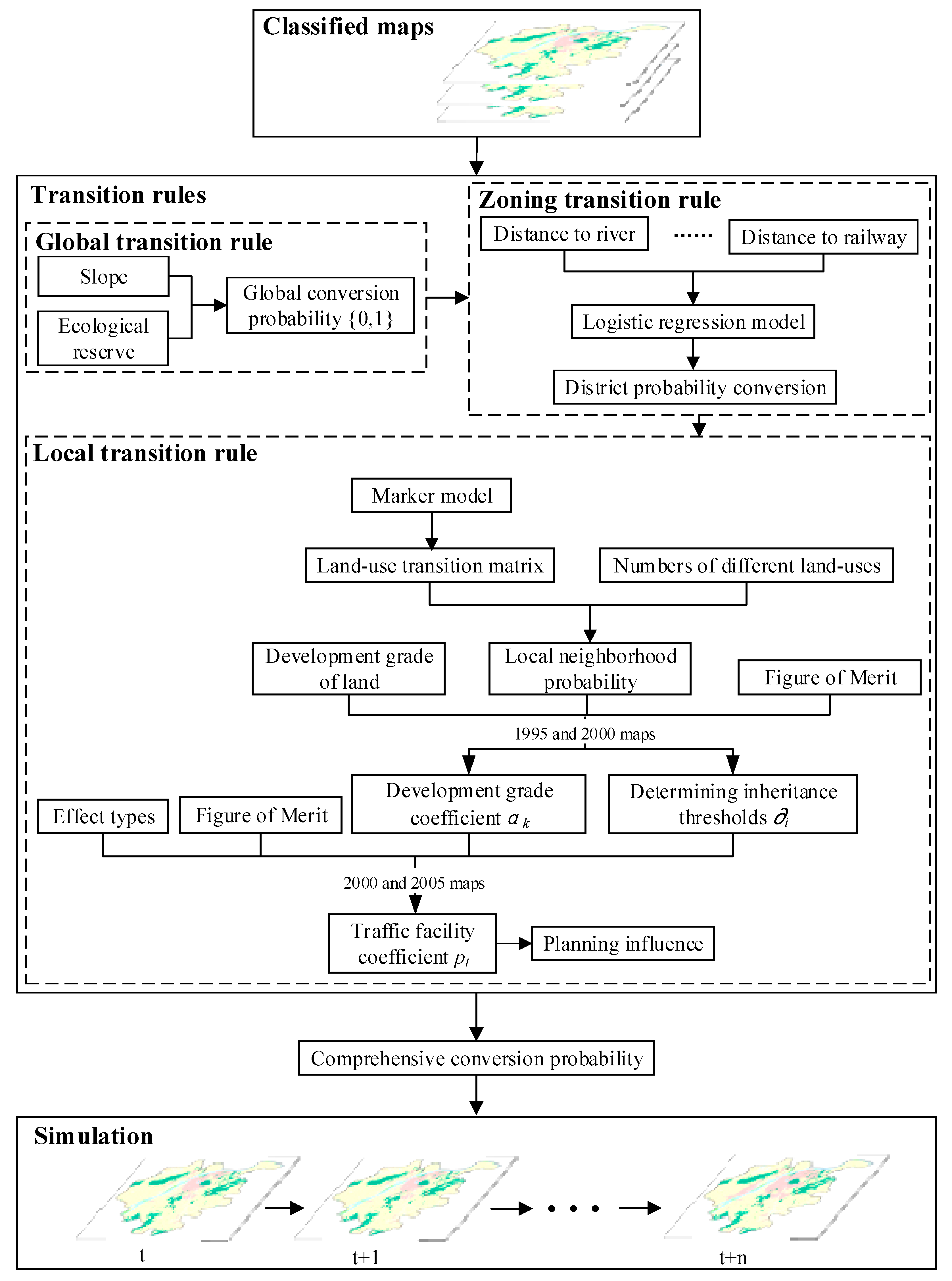
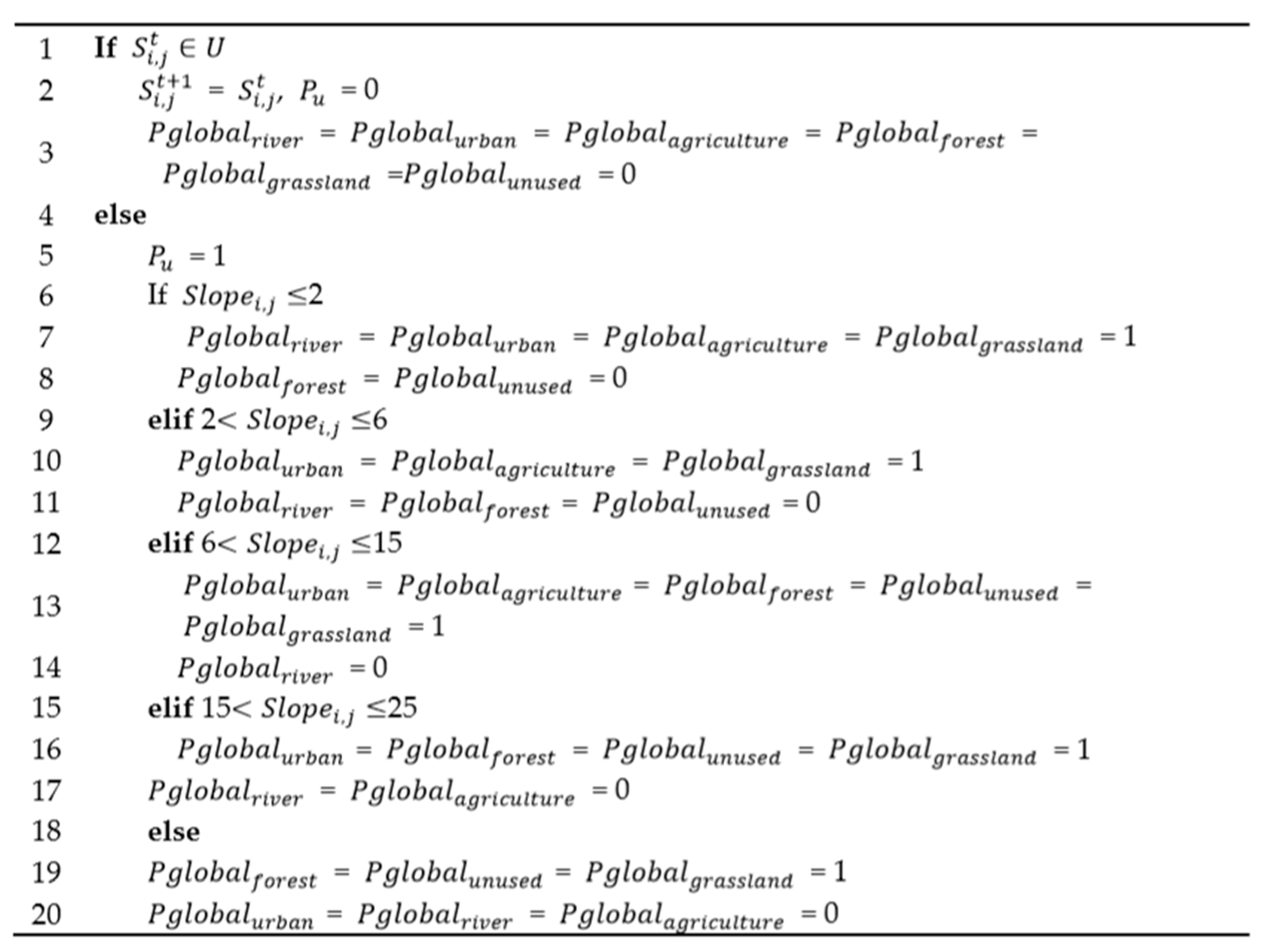
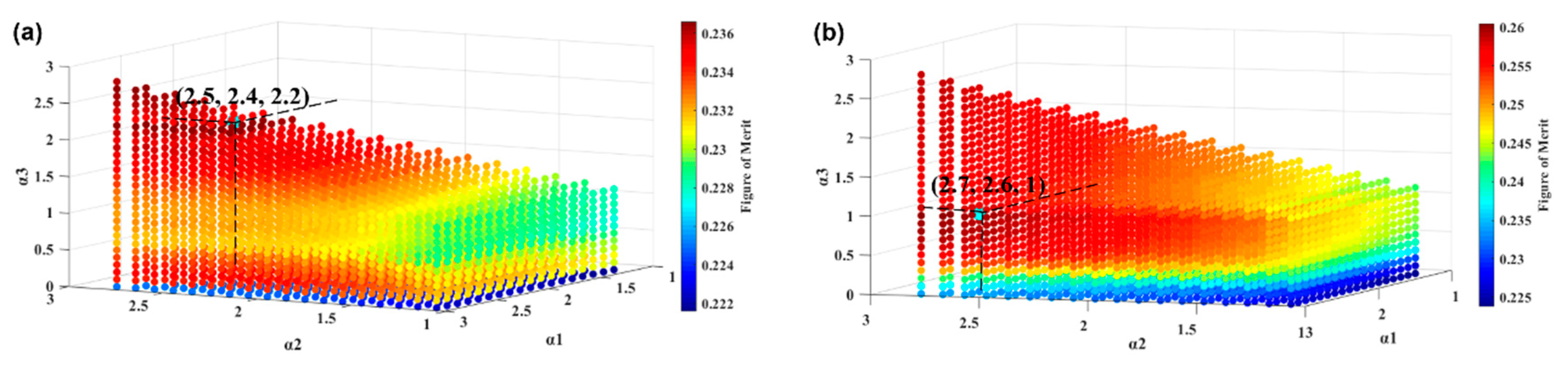
It is necessary to pay more attention to the adaptation of rules to real-world planning contexts [47]. Considering the spatiotemporal continuity and heterogeneity of urban development strategy, this paper proposes an urban development strategy-constrained CA model, which is combined with three transition rules. First, according to the slope and location (whether it is within the scope of the ecological reserve) of the central cell, the direction of its transformation can be judged. Second, considering the top-down characteristics and spatial heterogeneity of the implementation of the spatial layout, a special “zoning transition rule” is proposed by constructing evaluating functions to measure the suitability of different land types in different districts. Third, by adding the land development grade coefficient, the traffic facility coefficient and the time variable into the local conversion function, the dynamic and heterogeneous external intervention influence can be reflected in this model. Finally, whether the land use changes or not is dependent on the comprehensive probability of the above rules. Our experiment shows that the proposed model can effectively simulate the LUCC and that the control granularity of land use development is heterogeneous in different districts, which is reflected in the difference in the development grade coefficient. Moreover, the simulation results confirm that the design of the spatial layout is a comprehensive and all-round process which considered the spatial difference of the subway effect. Therefore, the addition of the traffic facility coefficient has not produced the expected results in this experiment. These findings suggest that we need to pay more attention to the guiding mechanism of the urban development strategy for urban sustainable development.

The remainder of this paper is organized as follows. In Section 2, we describe the study area, driving factors, the design of transition rules, the determination of parameters and the verification of the model. In Section 3, we present the case study experiment conducted in Nanjing. Section 4 discusses the experimental results. Section 5 presents our conclusions on the experimental results and proposes future work.

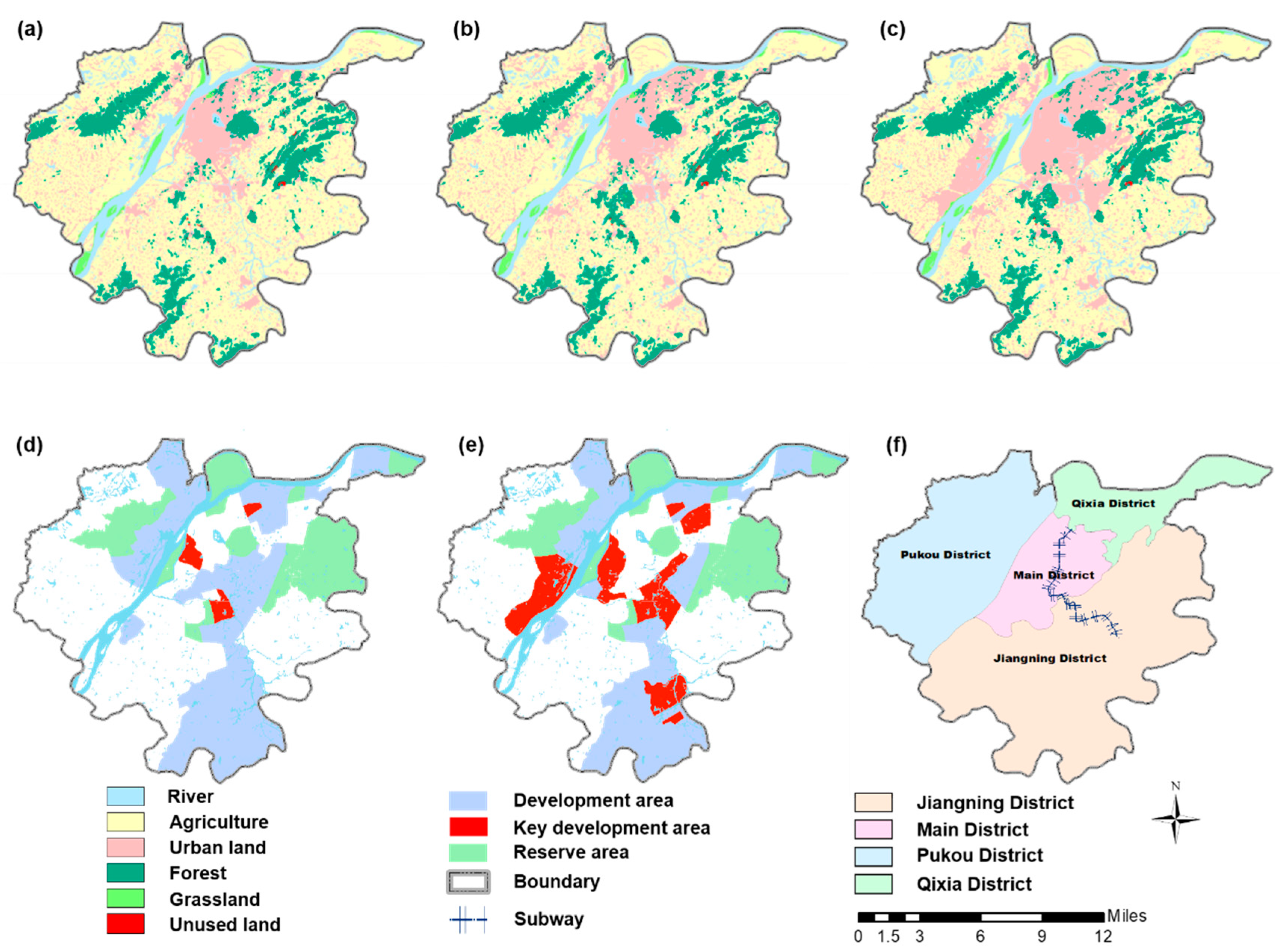
2. Materials and Methods

2.1. Study Area and Data Sources

The provincial capital—Nanjing city—is located in the southwest of Jiangsu Province. It is the central city in the middle and lower reaches of the Yangtze River. Its geographic coordinates are 118°22′–119°14′ E, 31°14′–32°37′ N. The projection of land-use dynamics was supplemented by analyses of land-use changes for the years 1995, 2000 and 2005, the Nanjing City Master Plan (1991–2010) (development grades of land use), the Nanjing city urban planning functional zoning (ecological reserve) and several driving factors (Figure 1 and

Table 1. LUCC driving factors adopted for different transition rules.

Types	Transition Rules	Driving Factors
Natural factors	Global transition rule	Slope
	Zoning transition rule	Distance to river (DtoR)
		Elevation
Traffic factors	Zoning transition rule	Distance to the national highway (DtoNH)
		Distance to the provincial highway (DtoPH)
		Distance to the first-class highway (DtoFH)
		Distance to the railway (DtoRl)
		Distance to the motorway (DtoM)
	Local transition rule	Distance to the subway
Urban factors	Zoning transition rule	Distance to the city centre (DtoCC)
		Distance to the county centre (DtoCoC)
		Distance to the town centre (DtoTC)
Planning factors	Global transition rule	Ecological reserve
	Local transition rule	Grade of land-use development

). The classified maps that were obtained from the Geographical Information Monitoring Cloud Platform [48], include six thematic land-use classes (river, forest land, agricultural land, urban and rural residential land, grassland and unused land), which were mapped at a spatial resolution of 30 × 30 m. The overall classification accuracy of the agricultural land and urban and rural residential land are more than 85%, and that of other types of land-use are more than 75%. According to the zoning policy, the main study areas are the urban areas of Nanjing city, which are divided into Qixia District, Main District, Jiangning District and Pukou District. The Nanjing Metro Line 1 began construction in 2000 and officially began operation on 3 September, 2005. It runs through the Qixia District, Main District and Jiangning District.

2.2. LUCC Driving Factors

There are two main forms of LUCC: the transition of land-use types and the change of land-use intensity. Generally, the driving force and cause, which result in those land-use dynamics, are called te LUCC driving factors. In this paper, the LUCC driving factors are divided into four types: natural factors, traffic factors, urban factors, and planning factors (Table 1).

2.3. Transition Rules

Transition rules are the key of the CA model, which is used to determine the state of the cell at the next moment based on the current state of the target cell and its neighbourhood cells. Liu [49] found that the simulation result would be better when the iteration number is an integer multiple of the observation, so we set the iteration number from 1995 to 2005 as 40. The design of the rules should penetrate three levels of the urban planning system (global, zoning and local) and follow a series of principles of land-use change. In this paper, we proposed a spatiotemporal difference-constrained CA model whose whole process is shown in Figure 2.

2.3.1. Global Transition Rule

As the first rule among all transition rules, the global transition rule remaining stable in a specific period is a constant variable that is not affected by the region and time, and its probability is commonly defined as the set of {0, 1}. When the probability value is 0, it means that it is impossible to convert the land-use type into a specific land-use type, so the other rules will not work; otherwise, land use meets the primary conditions for the conversion to a specific type. In this paper, there are the following two global constraints.

Slope Constraints

Slope is the ratio of the vertical height to horizontal distance of each cell, indicating the inclination degree. Different types of land use have different slope requirements. Here, there are two main kinds of slope constraints: the planning mandatory constraint and the analytical constraint.

(1) Planning mandatory constraint: in the code for vertical planning on urban field [50], the slope of urban and rural residential land must be less than 25°.

(2) Analytical constraint: taking classified maps for the years 1995 and 2000 as examples, land slope maps and classified maps are overlapped to analyse the slope constraints of other types of land use that are without mandatory planning constraints. According to the specifications for base-map production of the second national land investigation [51], the slopes of urban land use are divided into five levels for statistics, namely ≤2°, 2~6°, 6~15°, 15~25°, and >25°. Then, the slope distribution index (Equation (1)) is used to analyse the dominant slopes of different types of land use.

$$P=\frac{A_{ij}\times A}{A_i\times A_j}$$

(1)

where $A_{ij}$ is the total area of the $i\mathrm{th}$ type of land use with the $j\mathrm{th}$ level of slope, $A$ is the total area, $A_i$ is the total area of the $i\mathrm{th}$ type of land use, $A_j$ is the total area of the $j\mathrm{th}$ level of slope, and $P$ is the slope distribution index. With the increase of $P$, the dominance of the $i\mathrm{th}$ type of land use on the $j\mathrm{th}$ level of slope also increases. When $P$ is greater than 1, it indicates that the $i\mathrm{th}$ type of land use is suitable to generate on the $j\mathrm{th}$ level of slope. The specific dominance is shown in

Table 2. The slope dominance of different land-use types in 1995.

Slope	The Types of Land Use
	River	Agricultural Land	Residential Land	Forest Land	Grassland	Unused Land
0–2	3.749715	0.831182	0.635183	0.33193	1.666305	0.194276
2–6	0.531526	1.157626	1.068633	0.490533	0.889708	0.510358
6–15	0.4847	1.004208	1.144227	1.155114	0.854234	1.297419
15–25	0.529827	0.468231	0.671574	4.302906	0.992741	4.15173
>25	0.423168	0.171718	0.266865	6.362546	0.916602	3.593295

and

Table 3. The slope dominance of different land-use types in 2000.

Slope	The Types of Land Use
	River	Agricultural Land	Residential Land	Forest Land	Grassland	Unused Land
0–2	3.849988	0.882763	0.672931	0.252777	1.665558	0.159312
2–6	0.562731	1.225256	1.108991	0.38004	0.905429	0.418503
6–15	0.511673	0.950711	1.088816	1.314651	0.867801	1.406244
15–25	0.535038	0.396583	0.619102	3.61699	0.960287	3.324652
>25	0.442164	0.143669	0.304322	4.852855	0.905072	2.946072

. The dominant slopes of river, agricultural land, forest land, and unused land, with slopes of $P$ greater than 1, are less than 2°, less than 15°, greater than 6° and greater than 6°, respectively. The dominance of grassland with different slopes is greater than or close to 1; in other words, the grassland has no global slope constraints.

Ecological Reserve Constraints

In the process of urban construction, forest, grassland, agricultural land and river area are constantly transformed into urban and rural residential land for maximizing economic benefit, which leads to the destruction of urban ecosystems and the erosion of urban ecological function areas. To maintain regional ecological security and sustainable development of the economy and society, the state has delimited ecological reserve (Figure 1d,e), where the type of land used for forest, grassland or river remains unchanged. Otherwise, the type of land use will be converted when the transition probability exceeds the threshold.

In summary, the global transition rules are as follows (see Figure 3):

Where $S_{i,j}^t$ is the land-use type of the grid in row $i$ and column $j$ at time $\mathrm{t}$, and $S_{i,j}^{t+1}$ is the land-use type at time $\mathrm{t}+1$. $\mathrm{U}$ is a set of ecological reserves, including forest, grassland or river areas. $Slop{e}_{i,j}$ is the slope of the grid in row $i$ and column $j$. $P_u$ is used to determine whether the grid is within the scope of the ecological reserve. When the grid is within the scope, its state remains unchanged with $P_u$ being 0, and its probability of being converted to other types of land-use ($Pgloba{l}_{river}$, $Pgloba{l}_{urban}$, $Pgloba{l}_{agriculture}$, $Pgloba{l}_{forest}$, $Pgloba{l}_{grassland}$, $Pgloba{l}_{unused}$) is all 0. Otherwise, $P_u$ is 1, and the probability of being converted is determined according to the value of $Slop{e}_{i,j}$. The probability is 1, which means it is possible to be converted into this type of land, or the probability is 0, which means it is impossible to be converted into this type of land.

2.3.2. Zoning Transition Rule

After meeting the first transition rule ($P_u$ = 1), this paper notes that a new zoning transition rule needs to be considered in the CA model. As the management and control unit in zoning planning, districts are set as study sub-units to analyse the suitability of different land-use types by using a logistic regression model (Equation (2)). Therefore, we consider 10 factors (nature, traffic and urban factors) (in Table 1) to construct the zoning transition rule.

$$Pmiddl{e}_j=\frac{\exp \left({\beta }_0+{\beta }_1{X}_1+{\beta }_2{X}_2+\dots +{\beta }_n{X}_n\right)}{1+\exp \left({\beta }_0+{\beta }_1{X}_1+{\beta }_2{X}_2+\dots +{\beta }_n{X}_n\right)}$$

(2)

where $X_1$, $X_2$, …, $X_n$ are the driving factors; ${\beta }_1$, ${\beta }_2$, …, ${\beta }_n$ are the regression coefficients; and ${\beta }_0$ is the constant term. The regression coefficients and the constant term are different in different districts. $Pmiddl{e}_j$ is the probability of being the land-use type $j$, which is also defined as the suitability of the land-use type $j$ by some scholars.

2.3.3. Local Transition Rule

Neighbourhood Constraint

In urban development, the distribution of planning land is affected by the types of land uses in the neighbourhood of the candidate areas where the land may be developed. Therefore, the CA model always follows the principle that the types of central cells are affected by spatial neighbouring cells.

This model chooses the commonly used extended Moore neighbourhood of the 5 $\times$ 5 window; each cell represents an area of 50 m $\times$ 50 m on the ground for the simulation. In the neighbourhood window, land types of the other cells except the central cell are recorded and set as $DevelopNum$ = {$Lan{d}_{river}$, $Lan{d}_{agriculture}$, $Lan{d}_{urban}$, $Lan{d}_{forest}$, $Lan{d}_{grassland}$, $Lan{d}_{unused}$}, where $Lan{d}_{river}$, $Lan{d}_{agriculture}$, $Lan{d}_{urban}$, $Lan{d}_{forest}$, $Lan{d}_{grassland}$, and $Lan{d}_{unused}$ represent the numbers of the different types of land use. In general, the greater the number of certain land-use types in the neighbourhood, the greater the probability that the central cell will be converted into this land-use type; that is, the more likely the central cell will be assimilated. However, the number of land-use types in the neighbourhood is not the only criterion of local constraints. According to the construction demand and the change of national conditions, the transfer rates among different land-use types are different. They are obtained using the Markov model and saved as a land-use transition matrix $DevelopExtent$, where $R_r$,$A_a$,$R{U}_{ru}$,$F_f$,$G_g$,$\mathrm{and} U_u$ are the inheritance degree of the original land-use types, and the other parameters indicate the evolution degree in the transformation direction of the different land-use types. For instance, $R_{ru}$ indicates the evolution probability of river area being converted into urban area (Equation (3)).

$$\begin{gathered} riveragriurban\mathrm{forest}grassunused \\ \mathrm{DevelopExtent}=\begin{array}{c}river\\ agri\\ urban\\ forest\\ grass\\ unused\end{array}\left[\begin{array}{cccccc}{R}_r& R_a& R_{ru}& R_f& R_g& R_u\\ A_r& A_a& A_{ru}& A_f& A_g& A_u\\ R{U}_r& R{U}_a& R{U}_{ru}& R{U}_f& R{U}_g& R{U}_u\\ F_r& F_a& F_{ru}& F_f& F_g& F_u\\ G_r& G_a& G_{ru}& G_f& G_g& G_u\\ U_r& U_a& U_{ru}& U_f& U_g& U_u\end{array}\right] \end{gathered}$$

(3)

In addition, the land-use transition matrix that was obtained based on the classified maps for the years 1995 and 2000 is the initial matrix. In the iteration process, the matrix will change dynamically according to the evolution state of the land use in the last two moments. When the land type of the central cell is $i$ and the numbers of the different land-use types within the neighbourhood of the $\mathrm{n}\ast \mathrm{n}$ window are recorded in the matrix $DevelopNum$, then its local neighbourhood probability of being converted into the other land-use types ($Plocal{n}_{i\to j}$) is as follows:

$$DevelopExten{t}_i= \{i_r, i_a, i_{ru}, i_f, i_g, i_u\},$$

(4)

$$Plocal{n}_{i\to j}=\frac{i_{j}Lan{d}_j}{n\ast n-1}.$$

(5)

Planning Dynamic Constraint

Metro planning will produce urban land spill-over and aggregation effects that can be quantified into the planning influence to represent the influence degree of metro planning policy, which is related to space and time. The planning influence is determined by the types of intraregional effects; when the spill-over effect occurs in the region, it indicates that the policy has a spatial damping effect on the development of the land use, so the traffic facility coefficient (TFC, $p_l$) is a negative value. When the aggregation effect is generated in the region, it signifies that the policy exerts a spatial pull on the development of land use, so the traffic facility coefficient ($p_l$) is a positive value. In the experiment, we divided the development of the study area into two stages; from 1995 to 2000 and from 2000 to 2005. If the subway did not produce any effects in the second stage, the growth rates of residential land in this stage should be equal to those in the first stage. That is, the relative growth rate (RGR) of the two stages is equal to 0. If the sign of RGR is negative with some ranges, it means that the subway generates the spill-over effect on the land use with these ranges. Reviewing the reference on the influence of a subway on urban land [52,53,54], this paper divides the research range of the traffic facility coefficients into six levels: 0–200 m, 200–500 m, 500–800 m, 800–1600 m, 1600–2400 m, and 2400–3200 m. The experiment studies the dynamic change of the planning policy effect in the stage of subway construction. It is assumed that the policy effect has a linear relationship with time in the whole evolution process.

In addition, according to the Nanjing City Master Plan (1991–2010) and 2000 planning content adjustment text, the urban land is divided into three development grades (Figure 1d,e). The key development area, development area and other land belong to the first, second and third grades, respectively, and correspond to different development grade coefficients ${\alpha }_k$(${\alpha }_1, {\alpha }_2, {\alpha }_3$). The specific equation is shown as follows:

$$Plocal{p}_{k,l,t}={\alpha }_k(1+p_l\frac{t-t_s}{t_e-t_s})$$

(6)

where $Plocal{p}_{k,l,t}$ is the planning influence, $p_l$($p_1, p_2, p_3, p_4, p_5, p_6$) is the traffic facility coefficient (when the region is affected by the planning spill-over effect, it is a negative value, or not a positive value),${\alpha }_k$(${\alpha }_1, {\alpha }_2, {\alpha }_3$) is the development grade coefficient, which is decided by the development grade, $t_e$ and $t_s$ are the end time and start time of the planning policy, respectively, and $t$ is the current time of planning implementation.

In summary, the calculation of the local dynamic conversion probability ($Ploca{l}_{i\to j,k,l,t}$) is as follows:

$$Ploca{l}_{i\to j,k,l,t}=\{\begin{array}{c}Plocal{n}_{i\to j}\times Plocal{p}_{k,l,t} j=urban, t\ge t_s\\ Plocal{n}_{i\to j}\times Plocal{p}_{k,l,t} and p_l=0 j=urban, t\le t_s\\ Plocal{n}_{i\to j} j=others\end{array}.$$

(7)

2.3.4. Comprehensive Transition Rule

According to Wu [55], the comprehensive conversion probability ($Pcom{p}_{i\to j, k,l,t}$) can be obtained by combining the above transition rules (Equation (8)) as follows:

$$Pcom{p}_{i\to j, k,l,t}=P_u\times Pgloba{l}_j\times Pmiddl{e}_j\times Ploca{l}_{i\to j,k,l,t}.$$

(8)

Each cell has six conversion probabilities of being converted to different types of land use. There are six inheritance thresholds—${\partial }_{river}, {\partial }_{agriculture}, {\partial }_{urban}, {\partial }_{forest}, {\partial }_{grassland}, and {\partial }_{unused}$—in the model. When the inheritance value of a cell whose land-use type is $i \left(Pcom{p}_{i\to i,k,l,t}\right)$ and is greater than the threshold ${\partial }_i$, the land-use type remains unchanged. Otherwise, the cell will be transited to the land type $j$ with the greatest conversion probability (Max($Pcom{p}_{i\to j,k,l,t})$).

2.4. Model Parameter Estimation and Accuracy Verification

The figure of merit (FOM)—which consists of misses, hits, wrong hits and false alarms—is a popular metric for model validation by using three-map comparison, whose range is from 0 to 1. The closer the value is to 1, the more similar the simulated change is to the actual changes [56,57]. In this experiment, we used FOM to determine parameters and judge the simulation results.

There are three kinds of parameters that need to be set up in the model, including the inheritance thresholds (${\partial }_i$), development grade coefficients (${\alpha }_k$) and traffic facility coefficient ($p_l$). First, based on the reference map of 1995, we simulated the land-use changes in 2000 by calculating the six conversion probabilities of each cell without considering the planning influence. Comparing the simulation results with the actual map, the minimum conversion probabilities of each type of land-use without changes were what were defined as inheritance thresholds by us. Second, combined with the above obtained inheritance thresholds, the iteration method was used to calculate the FOM under different combinations of development grade coefficients, and the combination with the maximum FOM was the optimal combination of development grade coefficients. The traffic facility coefficient is set as 0 in the process of determining the development grade coefficient because the planning policy had not been implemented during the period. Third, the sign of the traffic facility coefficient ($p_l$) can be determined by judging the effect types based on the relative growth comparison of urban land in different regions before and after the planning policy. Then, we applied the iteration method to test the optimal traffic facility coefficients of the different districts with a step size of 0.1. The FOM of the simulated result was the largest, as we used this optimal traffic facility coefficient.

3. Results

The global transition probability of every cell ($P_u\times Pgloba{l}_j$) can be obtained based on its location and slope, which has been introduced above. In the following, we explain how to determine the middle transition probability ($Pmiddl{e}_j$) based on a logistic regression model and calculate the local transition probability ($Ploca{l}_{i\to j,k,l,t}$) by using the Markov model and planning influence.

3.1. Logical Regression Coefficient

According to the introduction in Section 2.3.2, logistic regression models of four districts were built based on the 10 LUCC driving factors of the zoning transition rules in Table 1, and the regression coefficients of each district are shown in

Table 4. Logistic regression factors and their coefficient of different districts.

District	Factors	Land-Use Types
		River	Agricultural Land	Residential Land	Forest Land	Grassland
Main District	DtoFH	−0.945	1.948	0.569	—	−4.036
	DtoNH	0.386	−0.185	−0.249	−0.903	4.556
	DtoPH	—	0.529	−0.203	−1.303	−1.911
	DtoRl	—	0.573	—	−0.438	−1.182
	DtoM	−0.717	—	0.745	—	5.421
	DtoCC	2.030	—	−2.267	−2.056	—
	DtoCoC	−1.249	—	—	2.028	—
	DtoTC	0.267	—	—	0.346	3.369
	DtoR	—	−0.218	0.810	−0.218	—
	Elevation	−3.372	−0.518	−0.898	2.040	1.287
	Constant	−1.520	−0.509	−0.101	−1.707	−5.297
Qixia District	DtoFH	5.751	−3.080	4.934	—	21.998
	DtoNH	—	1.993	−0.755	—	−19.279
	DtoPH	−4.766	4.104	—	—	−11.763
	DtoRl	−1.705	−2.169	—	−1.361	12.676
	DtoM	11.319	−5.574	1.677	—	39.650
	DtoCC	−4.282	3.193	−6.822	—	−17.897
	DtoCoC	−3.973	−0.962	0.578	—	−11.817
	DtoTC	0.657	—	—	—	0.853
	DtoR	—	0.839	0.585	0.454	−1.693
	Elevation	−1.756	−0.774	−0.132	1.985	0.820
	Constant	−1.545	0.080	−0.558	−2.15	−10.201
Pukou District	DtoFH	0.642	—	−0.663	−3.552	0.642
	DtoNH	—	−0.142	—	2.299	—
	DtoPH	0.761	−0.242	−0.471	—	−1.911
	DtoRl	−0.408	0.442	—	−0.653	0.761
	DtoM	—	—	—	—	—
	DtoCC	−2.738	3.082	—	2.889	−2.738
	DtoCoC	−0.274	—	0.734	—	−0.274
	DtoTC	2.309	−0.608	−0.125	−2.700	2.309
	DtoR	—	—	—	—	—
	Elevation	−3.433	−1.225	−0.433	4.303	−3.433
	Constant	−1.656	−0.036	−0.124	−1.707	−1.656
Jiangning District	DtoFH	−1.766	1.165	—	1.249	−4.511
	DtoNH	−0.760	—	−0.387	1.214	−1.984
	DtoPH	−0.335	—	−0.321	0.459	—
	DtoRl	1.795	0.952	—	−2.199	4.154
	DtoM	0.736	−0.638	—	—	—
	DtoCC	—	0.603	—	—	—
	DtoCoC	—	—	—	—	—
	DtoTC	0.349	−0.584	—	—	5.843
	DtoR	—	0.316	0.170	—	−0.453
	Elevation	−0.637	−1.609	−0.395	3.894	0.760
	Constant	0.041	0.184	−0.009	0.888	−2.320

. Since there is no change in the unused land, we only selected five types of land use to construct regression models.

3.2. Land-use Transition Matrices

Based on classified maps for the years 1995 and 2000, we obtained the initial land use transition matrices of four districts by using the Markov model (

Table 5. Land-use transition matrices of different districts.

District	Land-Use Types	Land-Use Types
		River	Agricult-Ural LAND	Resident-Ial LAND	Forest Land	Grassland	Unused Land
Main District	River	0.999	0.740	0.801	0	0	0
	Agricult-ural land	0.604	0.992	0.881	0.878	0	0
	Resident-ial land	0.575	0.777	0.999	0	0	0
	Forest land	0	0	0.833	0.998	0	0
	Grassland	0	0	0	0	1	0
	Unused land	0	0	0	0	0	1
Qixia District	River	0.999	0.620	0.620	0	0	0
	Agricult-ural land	0.732	0.994	0.889	0	0.773	0
	Resident-ial land	0	0.782	0.999	0.601	0	0
	Forest land	0	0.746	0.842	0.998	0	0
	Grassland	0	0.686	0.886	0	0.995	0
	Unused land	0	0	0	0	0	1
Pukou District	River	0.999	0.800	0.595	0	0	0
	Agricult-ural land	0.711	0.997	0.860	0.558	0	0
	Resident-ial land	0	0.654	0.999	0.583	0	0
	Forest land	0	0.620	0.743	0.999	0	0
	Grassland	0.643	0	0.764	0	0.999	0
	Unused land	0	0	0	0	0	1
Jiangning District	River	0.999	0.678	0.718	0.613	0.592	0
	Agricult-ural land	0.767	0.997	0.836	0.794	0	0
	Resident-ial land	0.743	0.681	0.999	0	0	0
	Forest land	0.659	0.632	0.797	0.999	0	0
	Grassland	0.648	0	0	0	0.999	0
	Unused land	0	0	0	0	0	1

). In the following table, every element represents the evolution probability between the different land uses, and the inheritance degrees of the original land-use types are all close to 1. Combining Equations (4) and (5), the neighbourhood conditions and the following transition matrices, we can obtain the local neighbourhood probability of every cell ($Plocal{n}_{i\to j}$).

3.3. Determination of Planning Influence

Planning influence ($Plocal{p}_{k,l,t}$) consists of the development grade coefficient (${\mathsf{\alpha }}_{\mathrm{k}}$) and the traffic facility coefficient (${\partial }_i$), which can be trained from the classified maps of 1995 and 2000 and of 2000 and 2005, respectively.

3.3.1. Development Grade Coefficient and Inheritance Thresholds

According to the planning text, there are ${\mathsf{\alpha }}_1$> ${\mathsf{\alpha }}_{2 }$> ${\mathsf{\alpha }}_3$. Based on the iterative method, the model accuracies (FOM) of the different districts are calculated under different combinations of grade coefficients. As shown in Figure 4, each point displays a combination of grade coefficients, and its colour represents the level of the FOM. The optimal combinations of Main District, Qixia District, Pukou District and Jiangning District are (2.5, 2.4, 2.2), (2.7, 2.6, 1), (-, 2.7, 2.5) and (2.3, 2.2, 1.9), respectively. That is, model accuracies are the largest when using those combinations. Based on the optimal combinations, we simulated the land use in 2000 by using the proposed model (Figure 5a).

By analysing

Table 6. The optimal development grade coefficient combinations and their inheritance thresholds of different districts.

District	${\mathbf{\alpha }}_{\mathit{k}}$			${\partial }_{\mathit{i}}$						FOM
	${\mathbf{\alpha }}_1$	${\mathbf{\alpha }}_2$	${\mathbf{\alpha }}_3$	${\partial }_1$	${\partial }_2$	${\partial }_3$	${\partial }_4$	${\partial }_5$	${\partial }_6$
Main District	2.5	2.4	2.2	0.001	0.452	0.049	0.191	0.345	0	0.2365
Qixia District	2.7	2.6	1	0.002	0.402	0.070	0.154	0.292	0	0.2605
Pukou District	—	2.7	2.5	0.005	0.450	0.219	0.113	0.190	0	0.2147
Jiangning District	2.3	2.2	1.9	0	0.377	0.145	0.449	0.500	0	0.1978

, it can be found that for Qixia District, the ${\mathsf{\alpha }}_1$ value is close to the ${\mathsf{\alpha }}_2$ value and quite far from the ${\mathsf{\alpha }}_3$ value. However, for Main District and Jiangning District, their grade coefficients are very close. Since there was no key development area in Pukou District in 1995, it only had two almost equal grade coefficients (${\mathsf{\alpha }}_2$ and ${\mathsf{\alpha }}_3$). For the four districts, their inheritance thresholds of river (${\partial }_1$) are all very small, which implies that it is hard for the river to be changed into other land. Almost all the inheritance thresholds of agricultural land (${\partial }_2$) and grassland (${\partial }_5$) are greater than 0.3, which may be due to the occupation of farmland and grassland for urban expansion. The inheritance threshold of forest land (${\partial }_4$) is obviously higher than that in other districts because a large number of forest lands adjacent to Main District in Jiangning District were cut down for district development. In addition, the inheritance thresholds of residential lands (${\partial }_3$) in Main District and Qixia District are clearly less than those in Pukou District and Jiangning District. Comparing the simulated result (Figure 5a) with the actual result (Figure 1a,b), we calculated the model accuracies (FOM), which are all greater than 0.19.

3.3.2. Traffic Facility Coefficient

The Nanjing Metro Line 1 began construction in 2000, so we should consider the traffic facility coefficient ($p_l$) in the simulation process from the 21st iteration. As shown in Table 6, the development grade coefficients and inheritance thresholds of the different districts were trained by using the data of 1995 and 2000. In 2000, Pukou District began to plan key development areas, and planning text specifies that ${\mathsf{\alpha }}_1$ must be larger than ${\mathsf{\alpha }}_2$, so we set ${\mathsf{\alpha }}_1$ to 2.8 in the next experiment. Through the signs of the relative growth rate of land use obtained by using the classified map of 1995, 2000 and 2005, it can be judged whether the subway has a spatial spill-over effect or spatial agglomeration effect on the land use within the different ranges. Then, we used the iterative method to simulate the LUCC and test the optimal TFC combinations. As shown in

Table 7. The relative growth rate (RGR), optimal traffic facility coefficient (TFC) combinations and FOM of different districts.

Level	Distance (m)	District
		Main District			Qixia District			Jiangning District
		RGR	TFC $\left({\mathit{p}}_{\mathit{l}}\right)$	FOM	RGR	TFC $\left({\mathit{p}}_{\mathit{l}}\right)$	FOM	RGR	TFC $\left({\mathit{p}}_{\mathit{l}}\right)$	FOM
1	0–200	−0.406	0	0.2106	0	0	0.2371	3.787	0	0.1890
2	200–500	0.308	0		−2.040	−0.1		2.651	0.1
3	500–800	−3.775	−0.1		−2.670	−0.2		2.081	0.2
4	800–1600	0.797	0.1		−2.008	−0.1		2.252	0.2
5	1600–2400	2.921	0.2		−2.881	0		0.603	0.1
6	2400–3200	1.300	0.1		3.794	0.2		0.710	0

, the subway produced a spill-over effect within 500 to 800 m of the Main District, but an aggregation effect within 800 to 3200 m. Jiangning District creates an aggregation effect within 200 to 2400 m. For Qixia District, the subway generates a spill-over effect within 200 to 1600 m, but an aggregation effect within 2400 to 3200 m. In summary, the aggregation effect coefficients or spill-over effect coefficients are all very small, less than or equal to 0.2. Comparing the simulated result (Figure 5b) with the actual result (Figure 1b,c), we found that the simulated accuracies (FOM) of Main District and Qixia District are both greater than 0.21, excepting the Jiangning District.

3.4. Simulation of LUCC

Combining the classified map and land development grade data of 2000 with the above obtained grade coefficients and thresholds, we used our proposed model to simulate what the land use will be like in 2005 without the traffic facility coefficient (subway effect) (Figure 5c).

We compared the simulation result (Figure 5c) with the actual result (Figure 1b,c) and calculated the FOM of the simulation result. As shown in

Table 8. The accuracy of the simulation results without the traffic facility coefficient in 2005.

	District
	Main District	Qixia District	Pukou District	Jiangning District
FOM	0.2296	0.2366	0.2145	0.1810

, the accuracies of the different districts are all above 0.18. Comparing the accuracies in Table 7 and Table 8, we found that they are almost the equal in Main District, Qixia District and Jiangning District. The result reflects that the subway effect on land use is negligible after considering the land development grade. This is because the planning process of land development is interactive and comprehensive—when classifying the spatial land development grade, the planning departments have considered the role of subway planning in land-use development. Therefore, the planning influence can be expressed only by the development grade, without a subway effect.

4. Discussion

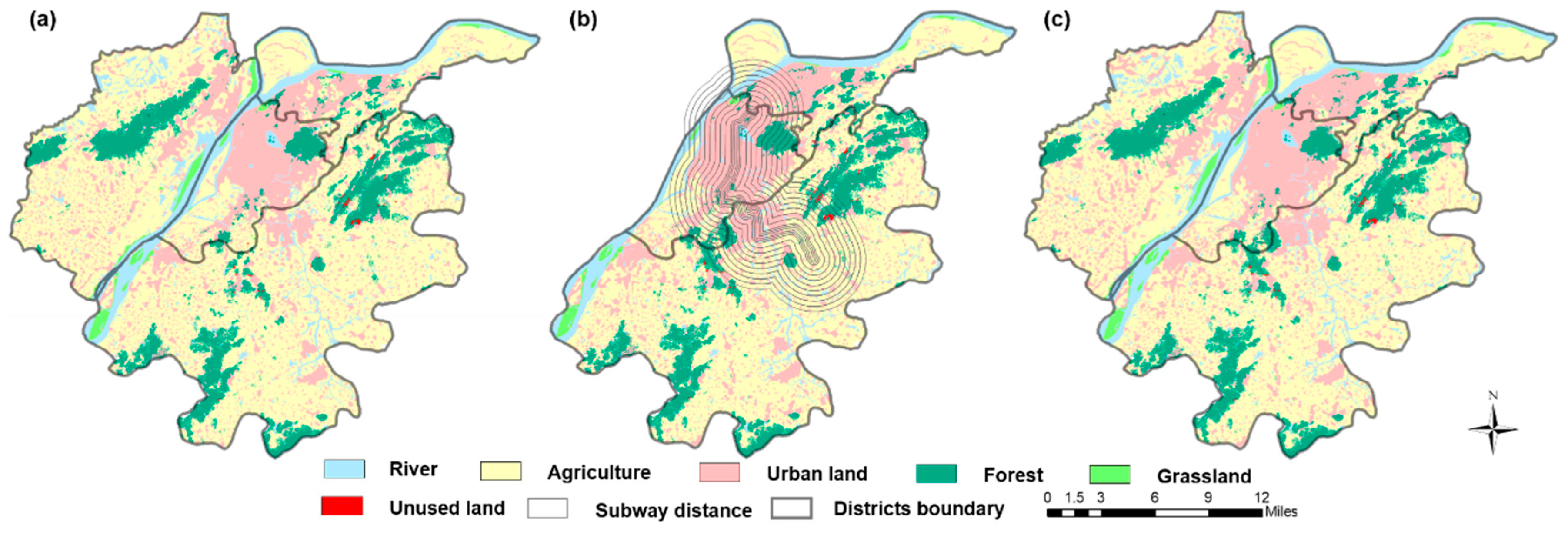
In fact, the differences in the grade coefficients of the districts—which are the land grade being different in one district and the coefficient of same land grade being different in different districts— reflect the differences in spatial control granularity of the land use. The form is due to the great differences in regional development and resource distribution, so the granularity of spatial development is heterogeneous. The latter is due to the characteristic of the Chinese planning system. where the management and control powers of different land-use grades are heterogeneous in different districts. As shown in Figure 6a,b, we also simulated what the urban land will be like without considering the development grade coefficients; in other words, we assume that the planning granularity of land development is homogeneous in the whole study area. Compared with Figure 5a,c, it is obvious that the residential lands of Figure 6a,b in the first and second development areas are larger, which confirms that the division of land grades has different driving forces for land expansion.

The simulation results (Figure 6a,b) are compared with the actual results (Figure 1b,c) to obtain the accuracies of the different districts. By comparing

Table 9. The accuracies of the simulation results without planning influence.

	Year	District
		Main District	Qixia District	Pukou District	Jiangning District
FOM	2000	0.2243	0.2315	0.2001	0.1956
	2005	0.2197	0.2034	0.2109	0.1711

with Table 6 and Table 8, it can be found that the simulation accuracies considering the differences in grade coefficients are almost higher. This conclusion further confirms that the differences in zoning control granularity are inevitable.

Further, comparing Figure 6b or Figure 5c with Figure 1c, it can be found that neither of the two simulation methods can simulate the residential land in the southwest of Pukou District (the scope circled in Figure 6b). This is due to the limitation of the CA model itself, which pays too much attention to the role of the neighbourhood. Although the planning department had designated this scope as a key development area in 2000, the original number of the residential land in this scope was too small to simulate the real development status.

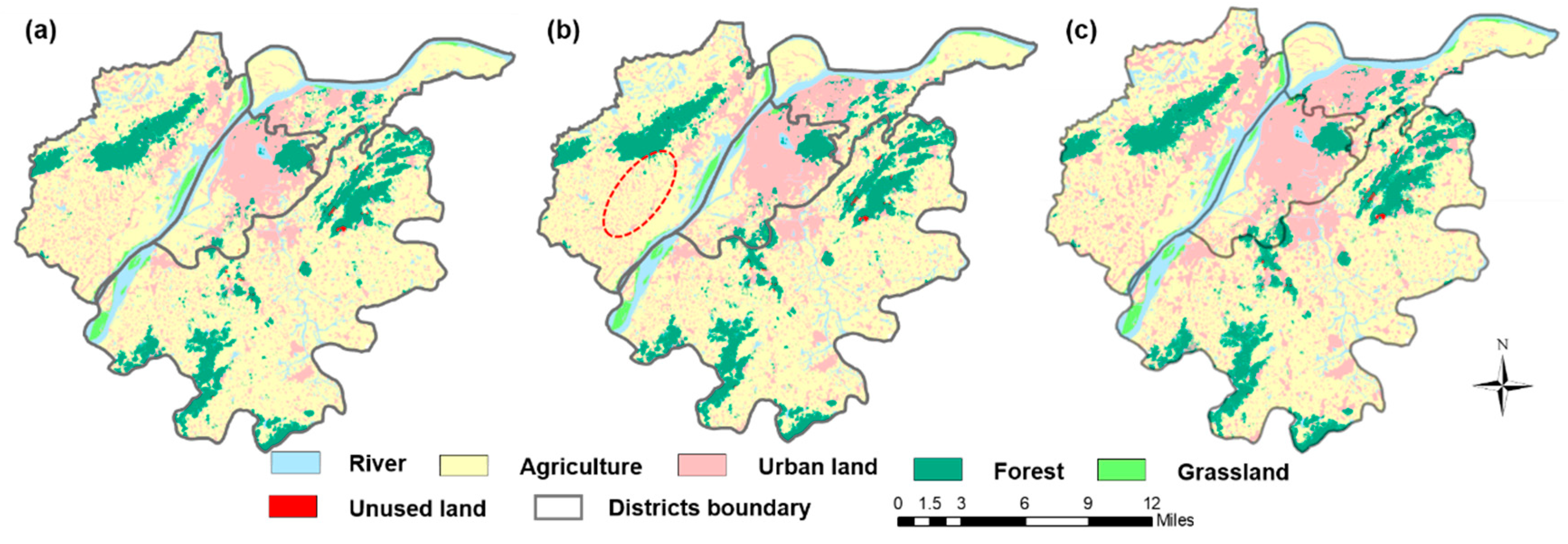
In addition, we simulated the land-use changes of Nanjing in 2020 based on the data of 2005 (Figure 6c). In the general land use planning of Nanjing (2006–2020), there are clear control indicators for the area of agricultural land, residential land and forest land in 2020. By comparing the simulated results with the planning indicators (

Table 10. The comparison of simulated results and planning indicators in 2020.

District	Land-Use Types
	Agricultural Land		Residential Land		Forest Land
	Simulated	Planning	Simulated	Planning	Simulated	Planning
Main District	1731.7	1480.5	20,710.7	25,281.1	2611	2270.8
Qixia District	16,189	14,803.7	10,504.7	12,943.8	4190.2	4207.7
Pukou District	58,058.25	57,611.7	14,914.5	17,438.5	20,603.5	20,488.5
Jiangning District	120,668.7	111,404.7	26,119.2	30,146.9	24,363.5	28,226.1

), we found that the overall results of the simulation were good, because the simulation results of each type of land-use reached 80% of the planning indicator. The simulation results of residential land in the four districts are less than the planning indicators, while the other two types of land-use are opposite. This finding indicates that the growth rate of residential land in the model is slightly smaller than that of planning. In other words—the development of residential land will accelerate between 2005 and 2020.

5. Conclusions

The urban development strategy plays an absolute guiding role in the process of urban land-use development. To simulate and discuss the development process of urban land use in a more real and objective way, this paper proposes a CA model under the constraint of the development strategy of urban planning. First, a new zoning transition rule is added to the two traditional rules to show the multi-level characteristics of the planning system. Second, the development grade coefficient is put out in the model to reflect the heterogeneity of the spatial control granularity in different districts. Third, we explored the spatial effects of subways by setting a traffic facility coefficient in the local transition rule. Through the above research, some significant results are summarized as follows:

• By comparing the simulation results of this proposed model and a model without considering the planning influence, it can be found that the heterogeneity of the spatial control granularity does exist and affects the simulation accuracies.
• Other contents of regulatory plans (e.g., road planning) have been taken into account in the design process of land-use spatial layouts, so the effect of subways on the simulation results in this model is very small.

People often define a city as a community that maintains a small scale for the good life. With the concepts of humanism and sustainable development becoming more and more popular, people are beginning to attach great importance to the living environment and comprehensive development of community. The results of this study suggest that planners can solve the problems of urban landscape fragmentation and achieve the goal of harmonious coexistence between man and nature by designating ecological reserves to establish continuous green grids and increase the continuity of urban green spaces. Based on the demand of people and the spatial distribution of infrastructure, planners can also realize intensive land use and develop compact cities by classifying the development level of land-use and controlling the granularity of different levels, thus reducing the use of resources and promoting urban sustainable development. Besides, we can simulate the land-use development under different planning strategies by using the model, and analysing the green, humanistic and sustainability of cities under different scenarios, so as to provide scientific guidance for the development of cities.

In cases where the residential land is too sparse to simulate the real development status, the proposed method revealed some limitations that must be resolved in future works. Apart from this, there are still some potential factors that need to be considered to better understand the driving mechanism of sustainable development. First, limited by the availability of data, this paper did not consider the influence of economic elements on the model, which need to be further studied. Second, the urban planning system is multi-level [19,28,29], and the system of each city is slightly different. Although this paper has considered the general level-zoning in order to simulate the process of land-use allocation more objectively—which is from the top to bottom—more levels need to be added. Third, urban population is the basis of land-use planning for planners, so we need to combine the population prediction model with the proposed model to improve the accuracy of urban growth simulation in the following work.

References

1. Heilig, G.K. World Urbanization Prospects: The 2011 Revision; United Nations, Department of Economic and Social Affairs (DESA), Population Division, Population Estimates and Projections Section: New York, NY, USA, 2012; p. 14. [Google Scholar]
2. Li, X.; Liu, X.; Yu, L. A systematic sensitivity analysis of constrained cellular automata model for urban growth simulation based on different transition rules. Int. J. Geogr. Inf. Sci. 2014, 28, 1317–1335. [Google Scholar]
3. Dahal, K.R.; Chow, T.E. An agent-integrated irregular automata model of urban land-use dynamics. Int. J. Geogr. Inf. Sci. 2014, 28, 2281–2303. [Google Scholar]
4. Rafiee, R.; Mahiny, A.S.; Khorasani, N.; Darvishsefat, A.A.; Danekar, A. Simulating urban growth in Mashad City, Iran through the SLEUTH model (UGM). Cities 2009, 26, 19–26. [Google Scholar]
5. Heistermann, M.; Müller, C.; Ronneberger, K. Land in sight?: Achievements, deficits and potentials of continental to global scale land-use modeling. Agric. Ecosyst. Environ. 2006, 114, 141–158. [Google Scholar]
6. Wu, F. Calibration of stochastic cellular automata: The application to rural-urban land conversions. Int. J. Geogr. Inf. Sci. 2002, 16, 795–818. [Google Scholar]
7. Liu, Y. Modelling sustainable urban growth in a rapidly urbanising region using a fuzzy-constrained cellular automata approach. Int. J. Geogr. Inf. Sci. 2012, 26, 151–167. [Google Scholar]
8. Liu, X.; Li, X.; Shi, X.; Zhang, X.; Chen, Y. Simulating land-use dynamics under planning policies by integrating artificial immune systems with cellular automata. Int. J. Geogr. Inf. Sci. 2010, 24, 783–802. [Google Scholar]
9. Lu, Y.; Cao, M.; Zhang, L. A vector-based Cellular Automata model for simulating urban land use change. Chin. Geogr. Sci. 2015, 25, 74–84. [Google Scholar]
10. Shi, W.; Pang, M.Y.C. Development of Voronoi-based cellular automata-an integrated dynamic model for Geographical Information Systems. Int. J. Geogr. Inf. Sci. 2000, 14, 455–474. [Google Scholar]
11. Feng, Y.; Liu, Y. A heuristic cellular automata approach for modelling urban land-use change based on simulated annealing. Int. J. Geogr. Inf. Sci. 2013, 27, 449–466. [Google Scholar]
12. Couclelis, H. Cellular worlds: A framework for modeling micro—macro dynamics. Environ. Plan. A 1985, 17, 585–596. [Google Scholar]
13. He, C.; Okada, N.; Zhang, Q.; Shi, P.; Zhang, J. Modeling urban expansion scenarios by coupling cellular automata model and system dynamic model in Beijing, China. Appl. Geogr. 2006, 26, 323–345. [Google Scholar]
14. Hagoort, M.; Geertman, S.; Ottens, H. Spatial externalities, neighbourhood rules and CA land-use modelling. Ann. Reg. Sci. 2008, 42, 39–56. [Google Scholar]
15. Hansen, H.S. Quantifying and Analysing Neighbourhood Characteristics Supporting Urban Land-Use Modelling; Springer: Berlin/Heidelberg, Germany, 2008; pp. 283–299. [Google Scholar]
16. Hansen, H.S. Empirically derived neighbourhood rules for urban land-use modelling. Environ. Plan. B Plan. Des. 2012, 39, 213–228. [Google Scholar]
17. Moreno, N.; Ménard, A.; Marceau, D.J. VecGCA: A vector-based geographic cellular automata model allowing geometric transformations of objects. Environ. Plan. B Plan. Des. 2008, 35, 647–665. [Google Scholar]
18. Moreno, N.; Wang, F.; Marceau, D.J. A geographic object-based approach in cellular automata modeling. Photogramm. Eng. Remote Sens. 2010, 76, 183–191. [Google Scholar]
19. Batty, M. Cities and Complexity: Understanding Cities with Cellular Automata, Agent-Based Models, and Fractals; The MIT press: Cambridge, MA, USA, 2007. [Google Scholar]
20. Pinto, N.N.; Antunes, A.P. A cellular automata model based on irregular cells: Application to small urban areas. Environ. Plan. B Plan. Des. 2010, 37, 1095–1114. [Google Scholar]
21. Cohen, B. Urban growth in developing countries: A review of current trends and a caution regarding existing forecasts. World Dev. 2004, 32, 23–51. [Google Scholar]
22. Ferrás, C. El enigma de la contraurbanización: Fenómeno empírico y concepto caótico. Eure (Santiago) 2007, 33, 5–25. [Google Scholar]
23. Augustijn-Beckers, E.W.; Flacke, J.; Retsios, B. Simulating informal settlement growth in Dar es Salaam, Tanzania: An agent-based housing model. Comput. Environ. Urban Syst. 2011, 35, 93–103. [Google Scholar]
24. Sohl, T.L.; Sayler, K.L.; Drummond, M.A.; Loveland, T.R. The FORE-SCE model: A practical approach for projecting land cover change using scenario-based modeling. J. Land Use Sci. 2007, 2, 103–126. [Google Scholar]
25. Kok, K.; Winograd, M. Modelling land-use change for Central America, with special reference to the impact of hurricane Mitch. Ecol. Model. 2002, 149, 53–69. [Google Scholar]
26. El Yacoubi, S. Cellular Automata: 7th International Conference on Cellular Automata for Research and Industry, ACRI 2006, Perpignan, France, 20–23 September 2006, Proceedings; Science Business Media: Berlin, Germany, 2006. [Google Scholar]
27. Couclelis, H. From cellular automata to urban models: New principles for model development and implementation. Environ. Plan. B Plan. Des. 1997, 24, 165–174. [Google Scholar]
28. Liu, X.; Liang, X.; Li, X.; Xu, X.; Ou, J.; Chen, Y.; Li, Y.; Wang, S.; Pei, F. A future land use simulation model (FLUS) for simulating multiple land use scenarios by coupling human and natural effects. Landsc. Urban Plan. 2017, 168, 94–116. [Google Scholar]
29. Verburg, P.H.; Overmars, K.P. Combining top-down and bottom-up dynamics in land use modeling: Exploring the future of abandoned farmlands in Europe with the Dyna-CLUE model. Landsc. Ecol. 2009, 24, 1167. [Google Scholar]
30. Yang, X.; Chen, R.; Zheng, X.Q. Simulating land use change by integrating ANN-CA model and landscape pattern indices. Geomat. Nat. Hazards Risk 2016, 7, 918–932. [Google Scholar]
31. Onsted, J.A.; Clarke, K.C. Forecasting enrollment in differential assessment programs using cellular automata. Environ. Plan. B Plan. Des. 2011, 38, 829–849. [Google Scholar]
32. Ward, D.P.; Murray, A.T.; Phinn, S.R. Integrating spatial optimization and cellular automata for evaluating urban change. Ann. Reg. Sci. 2003, 37, 131–148. [Google Scholar]
33. Ministry of Housing, Communities & Local Government. Plain English Guide to the Planning System [EB/OL]. Available online: https://www.gov.uk/government/publications/plain-english-guide-to-the-planning-system (accessed on 10 May 2019).
34. Greater London Authority. The London Plan: The Spatial Development Strategy for London Consolidated with Alterations Since 2011 [R/OL]. Available online: https://www.london.gov.uk/what-we-do/planning/london-plan/current-london-plan/london-plan-2016-pdf (accessed on 10 June 2018).
35. Owens, D.W. Introduction to Zoning; Institute of Government University of North Carolina: Chapel Hill, NC, USA, 2001. [Google Scholar]
36. CoE [Council of Europe]. European Regional/Spatial Planning Charter–Torremolinos Charter. In Proceedings of the 6th Conference of the Council of Europe of Ministers Responsible for Spatial Planning (CEMAT), Torremolinos, Spain, 19–20 May 1983; Council of Europe: Strasbourg, France, 1983. [Google Scholar]
37. Faludi, A. A turning point in the development of European spatial planning? The ‘Territorial Agenda of the European Union’and the ‘First Action Programme’. Prog. Plan. 2009, 71, 1–42. [Google Scholar]
38. Arsanjani, J.J.; Helbich, M.; Kainz, W.; Bolooranic, A.D. Integration of logistic regression, Markov chain and cellular automata models to simulate urban expansion. Int. J. Appl. Earth Obs. Geoinf. 2013, 21, 265–275. [Google Scholar]
39. Guan, D.J.; Li, H.F.; Inohae, T.; Su, W.; Nagaie, T.; Hokao, K. Modeling urban land use change by the integration of cellular automaton and Markov model. Ecol. Model. 2011, 222, 3761–3772. [Google Scholar]
40. Jantz, C.A.; Goetz, S.J.; Donato, D.; Claggett, P. Designing and implementing a regional urban modeling system using the SLEUTH cellular urban model. Comput. Environ. Urban Syst. 2010, 34, 1–16. [Google Scholar]
41. Murakami, J.; Cervero, R. High-Speed Rail and Economic Development: Business Agglomerations and Policy Implications; UC Berkeley, University of California Transportation Center: Berkeley, CA, USA, 2012. [Google Scholar]
42. Willigers, J.; Van Wee, B. High-speed rail and office location choices. A stated choice experiment for the Netherlands. J. Transp. Geogr. 2011, 19, 745–754. [Google Scholar]
43. Garmendia, M.; Romero, V.; Ureña, J.M.; Coronado, J.M. High-speed rail opportunities around metropolitan regions: Madrid and London. J. Inf. Syst. 2012, 18, 305–313. [Google Scholar]
44. Gutiérrez, J. Location, economic potential and daily accessibility: An analysis of the accessibility impact of the high-speed line Madrid–Barcelona–French border. J. Transp. Geogr. 2001, 9, 229–242. [Google Scholar]
45. Vickerman, R. High-speed rail in Europe: Experience and issues for future development. Ann. Reg. Sci. 1997, 31, 21–38. [Google Scholar]
46. Ureña, J.M.; Menerault, P.; Garmendia, M. The high-speed rail challenge for big intermediate cities: A national, regional and local perspective. Cities 2009, 26, 266–279. [Google Scholar]
47. Torrens, P.M.; O’Sullivan, D. Cellular automata and urban simulation: Where do we gofrom here? Environ. Plan. B Plan. Des. 2001, 28, 163–168. [Google Scholar] [CrossRef]
48. Beijing Digital View Technology Co., Ltd. Geographical Information Monitoring Cloud platform [DS/OL]. Available online: http://www.dsac.cn/ (accessed on 1 October 2012).
49. Liu, X.; Li, X.; Ye, J.; He, J.; Tao, J. Using ant colony intelligence to mine the transformation rules of geographic cellular automata. Chin. Sci. (Ser. D Geosci.) 2007, 6, 824–834. [Google Scholar]
50. Ministry of Housing and Urban-Rural Development of the People’s Republic of China (MOHURD). Announcement of the Ministry of Housing and Urban-Rural Development on the Publication of the Industry Standard “Regulations for Vertical Planning of Urban and Rural Construction Land” [EB/OL]. Available online: http://www.mohurd.gov.cn/wjfb/201607/t20160722_228283.html (accessed on 1 August 2016).
51. Ministry of Natural Resources of the People’s Republic of China. Notice on the Review of the Second National Land Survey Slope Map and the Arable Land Field Coefficient [EB/OL]. Available online: http://www.mnr.gov.cn/gk/tzgg/200903/t20090302_1989991.html (accessed on 25 February 2009).
52. Cervero, R.; Kockelman, K. Travel demand and the 3Ds: Density, diversity, and design. Transp. Res. Part D Transp. Environ. 1997, 2, 199–219. [Google Scholar]
53. Atkinson-Palombo, C.; Kuby, M.J. The geography of advance transit-oriented development in metropolitan Phoenix, Arizona, 2000–2007. J. Transp. Geogr. 2011, 19, 189–199. [Google Scholar]
54. Bowes, D.R.; Ihlanfeldt, K.R. Identifying the impacts of rail transit stations on residential property values. J. Urban Econ. 2001, 50, 1–25. [Google Scholar]
55. Wu, F.; Webster, C.J. Simulation of land development through the integration of cellular automata and multicriteria evaluation. Environ. Plan. B 1998, 5, 103–126. [Google Scholar]
56. Pontius, R.G.; Boersma, W.; Castella, J.C.; Clarke, K.C.; de Nijs, T.; Dietzel, C.; Duan, Z.; Fotsing, E.; Goldstein, N.; Kok, K.; et al. Comparing the input, output, and validation maps for several models of land change. Ann. Reg. Sci. 2008, 42, 11–37. [Google Scholar]
57. Varga, O.G.; Pontius, R.G., Jr.; Singh, S.K.; Szabó, S. Intensity Analysis and the Figure of Merit’s components for assessment of a Cellular Automata–Markov simulation model. Ecol. Indic. 2019, 101, 933–942. [Google Scholar]
Figure 1. Illustration of the study area (Nanjing, China): (a) 1995 satellite-derived classified map; (b) 2000 satellite-derived classified map; (c) 2005 satellite-derived classified map; (d) 1995 urban land planning functional zoning; (e) 2000 urban land planning functional zoning; and (f) division maps of different districts and metro spatial layout.
Sustainability 11 04012 g001
Figure 2. Flowchart of the spatiotemporal difference-constrained CA model.
Sustainability 11 04012 g002
Figure 3. Main steps of the global transition rules.
Sustainability 11 04012 g003
Figure 4. The development grade coefficient combinations of different districts: (a) Main District; (b) Qixia District; (c) Pukou District; and (d) Jiangning District.
Sustainability 11 04012 g004aSustainability 11 04012 g004b
Figure 5. Simulation result of the LUCC: (a) in 2000 with the development grade coefficient; (b) in 2005 with the traffic facility coefficient; and (c) in 2005 without the traffic facility coefficient.
Sustainability 11 04012 g005
Figure 6. Simulation results: (a) without planning influence in 2000, (b) without planning influence in 2005, and (c) with planning influence in 2020.
Sustainability 11 04012 g006