Demand-Oriented Train Timetabling Integrated with Passenger Train-Booking Decisions

School of Traffic and Transportation Engineering, Central South University, Changsha 410075, China
*
Author to whom correspondence should be addressed.
Sustainability 2019, 11(18), 4932; https://0-doi-org.brum.beds.ac.uk/10.3390/su11184932
Submission received: 10 August 2019
/
Revised: 4 September 2019
/
Accepted: 5 September 2019
/
Published: 9 September 2019
(This article belongs to the Collection Sustainable Rail and Metro Systems)
Abstract
:In recent years, with the global energy shortage and severe environmental deterioration, railway transport has begun to attract great interest as a green transportation mode. One of the vital means to realize social sustainable development is to improve railway transportation systems, in which providing a demand-oriented train timetable with a higher service level is the most viable method. A demand-oriented train timetable problem generally deals with passengers’ train-choice decisions according to the queue principle, but it is not adapted to rail systems, such as China’s, where passengers usually book tickets a few days in advance by telephone or online instead of going to stations. This paper is devoted to modeling and solving the demand-oriented train timetabling problem integrated with passengers’ train-booking decisions. Firstly, a bi-level programming model is formulated for their integrated optimization on a rail network. Its upper-level model is to optimize train arrival and departure times at each visited station with the aim of reducing passengers’ total travel cost, while its lower-level model aims to determine passengers’ train-booking behavior using the user equilibrium theory. Then, a priority-based heuristic algorithm is designed to solve this model. It has two main steps at each iteration: one is to determine the number of passengers booking each train with a given train timetable, and the other is to improve the current train timetable based on the valuable information of passenger train-booking decisions. The performance, convergence, and practicability of the proposed method were analyzed based on the Changsha–Zhuzhou–Xiangtan intercity rail in China. Experimental results show the proposed method can effectively reduce the travel cost for passengers, creating a greater passenger demand for railway travel, which is beneficial to the sustainable development of railway systems and even society.
1. Introduction
A train timetable specifies the arrival and departure times of trains at stations on a rail network. It is not only the cornerstone of train organization and station operation, but also the foundation of passengers choosing trains for traveling. Facing the high requirements of passengers at a service-level and the fierce competition with expressway and air transport in the passenger market, railways have become less attractive to passengers. However, the railways are actually an important part of a green transportation system for social sustainable development as they have a large capacity, energy-saving, and environmental protection capabilities. Therefore, it is very important and urgent for rail enterprises to provide passengers with higher service-level train timetables. Firstly, this can attract more passengers to travel by rail instead of road and air, which can effectively reduce environmental pollution and energy consumption. Secondly, with the improvement of the service level of the train timetable, the transport market competitiveness of the railway will be further improved, which is beneficial for the sound development of railways. Moreover, a better train timetable will contribute to reducing the usage numbers of rail crews, locomotives or electric multiple units. In short, the service-level improvement of train timetables for passengers will necessarily contribute to the sustainable development of railway systems and society.
Nevertheless, most early existing studies about train timetabling have not fully integrated the consideration of the time-dependent origin-to-destination (OD) passenger demands in the train timetabling process, and have usually aimed to optimize a train timetable with the objective of reducing trains’ travel time or their delay at stations. This is partly due to the difficulty of determining passengers’ train-choices for each OD demand. For example, Higgins et al. [1] only aimed to obtain a train timetable with minimum train delay by reducing train dwell time at stations. Burdett et al. [2] minimized train travel time when optimizing train timetable using a hybrid job shop approach. Zhou et al. [3] built an integer linear programming model with many 0–1 binary and non-negative integer decision variables, and proposed a Lagrangian relaxation decomposition approach to minimize train travel time. Bešinović et al. [4] optimized train timetable with the goal of minimizing train travel time and used heuristic algorithms to solve the problem. Based on the construction of a weighted directed graph, Zhou et al. [5] proposed a multi-path searching model with the aim of minimizing the total travel time of all period-types of trains. As for reducing trains’ delay, Goverde [6] used a max-plus system theory to illustrate a rail timetable stability measure, and then further analyzed train delay propagation processes. Corman et al. [7] employed a bi-objective model aiming to minimizing trains’ delays for obtaining a set of feasible non-dominated schedules. Xu et al. [8] combined genetic algorithm into travel advanced strategy for finding a train timetable with the lowest delay ratio. In addition, some studies adopted minimizing total operating cost, maximizing total profit, etc. as the objective of train timetabling. For instance, Brannlund et al. [9] aimed to find a profit-maximizing train timetable. Robenek et al. [10] optimized the timetable with the goal of maximizing the revenue of operating company based on passenger satisfaction. Li et al. [11] tried to find a train timetable with the minimum energy consumption. Other studies focused on avoiding conflicts among trains in the process of timetabling; for example, Carey et al. [12] and Caimi et al. [13] developed microscopic models for finding and avoiding conflicts among trains with constraints of various operational needs. Dundar et al. [14] formulated a decision support tool to resolve inter-train conflicts for the single-track railway train re-scheduling problem.
Besides the many studies on rail train timetabling, many scheduling studies on roads, airplane fields, etc. are also worth mentioning. For example, Marguier et al. [15] used mathematical programming method and heuristic search algorithm to optimize the bus schedule under the condition of reduced fleet size. Herbon et al. [16] combined bus operation cost and passenger satisfaction to study the bus departure schedule problem. Yang et al. [17] designed a model to solve the timetable problem for Yizhuang Line of Beijing Metro by using genetic algorithm, which aims to reduce energy consumption. Zheng et al. [18] presented a model for emergency railway wagon scheduling with the aim of minimizing the weighted time of delivering all required supplies to affected areas. Dobson and Lederer [19] presented a model for airline choice of flight schedule and route prices to maximize profit considering competitors decisions. Jiang et al. [20] introduced a dynamic airline scheduling method, which showed that making minor adjustments to flight schedules in the booking period by re-fleeting and re-timing flight legs can significantly improve utilization of capacity and hence increase profit.
In recent years, the demand-oriented train scheduling problem has attracted much attention. This kind of problem, called demand-oriented train timetabling problem (DOTTP), is usually to find an optimal or satisfactory train timetable for minimizing the total cost of passengers such as in-vehicle time, wait time and transfer time. Parbo et al. [21] illustrated that the importance of creating a demand-oriented railway timetable consists in offering the best service for passengers under some limited resources. Therefore, it is necessary to consider the train-choice decisions of passengers in train timetabling. For instance, Yu et al. [22] and Ma [23] employed a bi-level programming model whose objective was to minimize passengers’ total travel time with the consideration of the route choice behaviors of the users. Wang et al. [24] employed a deterministic Frank–Wolfe loading approach to solve the problem of passengers’ route choice behavior. Cordone et al. [25] and Parbo et al. [26] presented a mixed integer nonlinear programming model to capture the feedback mechanism between transport offer and passenger demand. These studies on passengers’ train-choice usually regarded passengers’ train-choices as a feedback of current timetables, and applied it as a useful information for further improving this train timetable, while providing passengers better service based on the improved train timetable. This is particularly crucial nowadays for rail enterprises, which aim to minimize their total operating cost and maximizing total profit when facing the high requirement of passengers on service-level and the fierce competition from expressways and air transport. Therefore, some studies took the interests of both passengers and operators into account to optimize train timetables. For example, Kaspi et al. [27] and Canca et al. [28] presented a scheduling optimization model that takes both the user and the operator points of view into account. Yang et al. [29] focused on designing a passenger-oriented timetable to reduce the passenger travel time and energy consumption simultaneously. Other existing studies on passenger demand-oriented train scheduling mainly aimed to reduce the waiting times or the total travel times, which are two fundamentally important elements for designing timetables. As for reducing the waiting times, for example, Barrena et al. [30] proposed three formulations for the train-scheduling problem with the aim of minimizing the passenger waiting time and a branch-and-cut algorithm to design train schedules under a dynamic demand environment. Niu et al. [31] proposed nonlinear mixed integer optimization models for the train scheduling problem with the objective of minimizing the total passenger waiting time at stations under time-dependent passenger demand and predetermined stop-skipping patterns. As for minimizing the total travel times, for instance, Yang et al. [32] developed a two-stage stochastic integer programming model to minimize the expected travel time and penalty value incurred by transfer activities. Johan et al. [33] proposed combined microscopic simulation and macroscopic timetable optimization approach for minimizing travel time and delays in railway timetables. Zhang et al. [34] formulated two nonlinear non-convex programming models to design timetables with the objective of minimizing the total passenger travel time under the constraints of train operations, passenger boarding and alighting processes and congested conditions.
The problem of scheduling integrated with demands in road, airplane fields, etc. have also attracted more attention of researchers. For instance, Ibarra-Rojas et al. [35] developed a bi-objective, integer programming model to maximize the number of bus passengers benefiting from well-timed transfers and minimize vehicle operating costs. A more complex bi-objective and bi-level approach was presented by Liu et al. [36] and Liu et al. [37], who studied how much the changes on timetable and vehicle scheduling affect users’ trip choice behavior. Wang et al. [38] established a demands-matching orientated multiple criteria decision making method for reverse logistics, including weights derivation, rank of collection modes, sensitivity analysis, and quantification of demands matching degree. Jiang et al. [20] introduced the concept of dynamic flight scheduling with the objective is to match the passenger demand and aircraft capacity for all flights. Abdelghany et al. [39] explicitly considered competition among airlines and passengers’ demand elasticity by integrating an airline competition analysis model in the scheduling process that captures the passengers’ itinerary choice behavior to enable evaluation of the profitability of the developed schedule.
To summarize, most studies deal with the demand-oriented train timetabling problem decided passenger train-choices mainly according to the queue principle, thus these passengers should wait at stations for a train arriving and then get on it one by one until its capacity is reached. For instance, Niu et al. [40] assumed that all passengers boarding a train obey the First-In-First-Out (FIFO) principle; if passengers are not be able to board the next arrival train, then they are forced to wait in queues for the following trains. Barrena et al. [30] obtained the origin–destination matrices based on the available passenger arrival data between stations during each time interval, and then these ordered passengers waited at relative stations for trains to get on without exceeding the capacity of trains. Passengers who are not able to board the current train should wait at this station for the next train. Wang et al. [41] divided passenger flows into multiple sub-flows so that they can choose different platforms to wait for trains obeying the queue principle. Niu et al. [31] viewed passenger queues in the train timetabling problem as a bulk queue to compute the cumulative number of departure passengers at stations to minimize the total passenger waiting time. Wang et al. [42] considered trains run in a first-in first-out order from one station to another station, thus passengers traveling between two consecutive stations board a train one by one until the train’s capacity is achieved. In the accurate passenger flow control strategies Shi et al. [43] proposed, passengers under control are required to queue up outside the entrance facilities. Moreover, no passengers will give up their trips or select other transportation modes. Besides, a few studies distributed all passengers of each interval-based demand on their shortest cost path. For instance, Fu et al. [44] assumed that passengers select their most time-saving path from all the available routes in a train service network.
Obviously, such a condition of passengers arriving at origin station to buy tickets and then waiting in queue there for the earliest arrival available train is adapt to the rail system of many countries such as Japan. However, it does not happen for the rail system in China, where passengers usually book tickets one day or a few days in advance. They usually do not need to go to the station to book tickets, but purchase them using many other methods, such as telephone and online booking. After that, they go to origin stations dozens of minutes in advance for boarding their booked trains on time. Thus, passengers usually do not need to wait for a booked train, and their choices of booking trains depend on not only the total travel time and ticket fare from origin to destination, but also the deviation time, which is the absolute value of the difference between train’s departure time and passengers’ planned departure time. Generally, they prefer to book a train whose departure time at origin station is close to their planning departure time when having the same other costs. Although train-booking decisions is also a train-choice decision, it is different from that based on queue rules, e.g. it considers the deviation time, rather than the wait time at origin station. Therefore, the existing methods of deciding passenger train-choices based on queuing theory are not efficient for this case as they do not consider passengers’ ticket booking decisions.
This paper is devoted to solving the demand-oriented train timetabling problem (DOTTP) integrated with train-booking decisions of passengers in the planning stage. Specifically, we use the user equilibrium theory to simulate passengers’ train-booking decisions based on an obtained train timetable, combined with the simulation results, to optimize the train timetable at each iteration. The main contribution of our research is that we propose a method for optimizing train timetable combining with passenger’ train-booking decisions, and this method can be effectively adopted in rail systems that allow train booking. Compared to the existing literature, the following two specific contributions are provided in this paper:
- A bi-level programming model is built for the demand-oriented train timetabling problem, combining it with passenger’ train-booking decisions. Its upper-level model is intended to optimize train timetables, while its lower-level model focuses on determining the trains booked by passengers based on a given train timetable.
- A priority-based heuristic algorithm is designed to solve the proposed bi-level programming model. It has two main steps at each iteration, one is to determine the number of passengers booking each train with a given train timetable, and the other is to improve the current train timetable based on the valuable information of passenger’s train-booking decisions.
The rest of this paper is organized as follows. The problem definition is introduced in Section 2, a bi-level programming model of train timetabling is built in Section 3, and then its priority-based heuristic search algorithm is designed in Section 4. Moreover, the convergence, effectiveness and practicability of the proposed model and its solving algorithms are tested based on the Changsha–Zhuzhou–Xiangtan intercity railway in Section 5. Finally, conclusions and future studies are summarized in Section 6.
2. Problem Definition
2.1. Assumptions
Our research is based on the following two assumptions:
- We only concentrate on the problem of train timetabling on a double-track rail network, and suspend the train routing problem at stations; furthermore, stations are viewed as nodes without the restriction of the maximum number of trains there at the same time.
- The time-dependent demand of each origin–destination is discretized into many granularity-based demands through dividing the planning horizon into multiple time granularities with a length of 10 min or another required time interval, and the planned departure time of each granularity-based demand is the middle time of its corresponding time period. For example, demands of granularity from 8:00 to 8:10 have the same planned departure time of 8:05.
2.2. Inputs and Outputs
The inputs of DOTTP include the rail network, period-based demands, and a set of trains whose arrival and departure times at stations are unknown.
- The rail network is composed of a set of station nodes and a set of rail one-way sections. Moreover, the operation time-horizon of the trains and some other related parameters of this rail network such as the mileage of rail section are given.
- Passenger demands are discretized into many period-based demands, and, thus, the origin, terminal, and passenger number of each period-based demand are given.
- The origin, terminal, and visited stations of each train are given; however, its stops and timetable are also needed for our research. Moreover, operation parameters such as the minimum required travel times in each rail section and dwell time at stations are also given.All symbols defined for expressing the input data of DOTTP are introduced in Table 1.
The definitions of the outputs, namely, the decision variables of DOTTP, are given in Table 2.
3. Bi-Level Programming Model of Demand-Oriented Train Timetabling Problem (DOTTP)
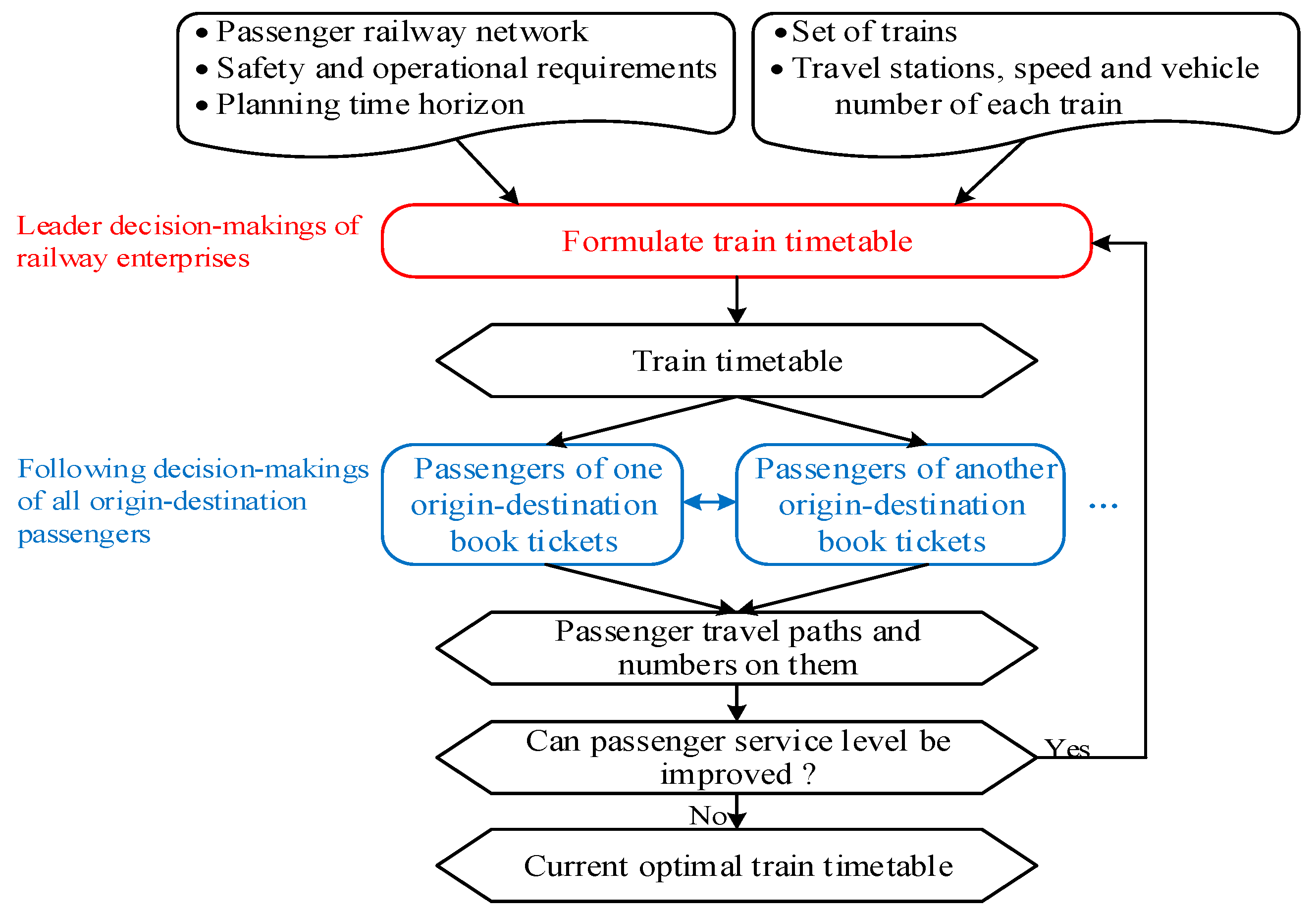
The DOTTP involves the decision-making of both rail enterprises and passengers, and the way they influence each other is shown in Figure 1. First, rail enterprises formulate a timetable with a set of trains based on a given rail network and many safety and operation restrictions, which is regarded as leader decision-making. Then, passengers have to book tickets of one or more specific trains to travel from origins to destinations based on this formulated train timetable, which involves multiple follow-up decisions. Passengers’ follow-up decisions can be viewed as feedback to the leader decisions of rail enterprises. Generally, it is very effective for rail enterprises to improve their previous formulated train timetable, i.e., leader decisions, according to the feedback. Accordingly, that adjustment of the leader decisions will further lead to the changes to passengers’ follow-up decisions. In reality, the alternate adjustment of the leader and following decisions may last for a long time until passenger service level cannot be improved further, but it also may be terminated for some reason, for example, the constant change of demands. The leader–follower hierarchical relationship of decision-making between railway enterprises and passengers can be described as a bi-level programming model, consisting of an upper-level model for train timetabling detailed in Section 3.1 and a lower-level model for distributing passengers to trains, as introduced in Section 3.2.
3.1. Upper-Level Model for Train Timetabling
Taking a double-track rail network and a set of trains whose visited stations, speed, and rated passenger capacities are predetermined, the upper-level model (UM) focuses on determining the arrival and departure times of trains at stations in the planning horizon to form a train timetable with the aim of minimizing the total travel time of passengers and the constraints of the safety time-interval of trains.
Based on the notations and decision variables detailed in Table 1 and Table 2, respectively, we formulate the objective of UM as minimizing the summation of products of passenger number and travel time on paths, namely,
The first part in the square bracket represents passenger in-vehicle time on path p, the second part expresses the deviation time between the train departure time and passenger planned departure time at origin on path p, and the third part is the transfer time at transfer stations, respectively, on path p. Note that the passengers can book trains that depart earlier or later than their planned departure time, thus the deviation time in the second part needs to be taken as its absolute value.
In addition, the following five types of constraints are considered in UM.
3.1.1. Constraints of Train Travel Time in Sections
The train travel time in each section is composed of pure running time and additional time for starting and stopping depending on whether this train stops at the inbound and outbound stations. That is,
3.1.2. Constraints of Train Minimum Dwell Time at Stations
Train dwell time at each station should be sufficient for passengers to get on and off it, namely,
For example, Table 3 shows the minimum dwell time of trains at stations with different numbers of passengers on a Japanese high-speed railway. However, it does not indicate that we only take this factor into account, other influencing factors are actually reflected in the stopping time, such as fixed time values. We use the minimum dwelling time without limiting the upper value, if the train needs to carry out technical work at a station, the dwelling time can be extended appropriately.
3.1.3. Safety Interval Constraints between Train Departure Time
The headway between two trains driving into either the same section or two different sections from the same station should not be less than the safety departure interval, that is,
3.1.4. Safety Interval Constraints between Train Arrival Time
Similarly, the headway between two trains arriving at a station from either the same section or two different sections should not be less than the safety arrival interval, namely,
3.1.5. Value Range Constraints of Train Arrival and Departure Time
The values of train arrival and departure time must be within the given planning horizon. That is,
As for safety interval constraints (Section 3.1.3 and Section 3.1.4), it is worth noting that the headway between two trains driving into two different sections from the same station or arriving at a station from two different sections is not necessary. Only when two trains occupy the same throat zone at a station should the safety headway be taken into consideration; otherwise, the headway is set as 0.
In the above UM, the calculation of objective in Equation (1) needs the passenger numbers of all chosen paths, and the minimum dwell time of trains at stations in safety interval constraints between train departure time (Section 3.1.3) depends on the total numbers of passengers getting on and off them at the stations. Those required passenger numbers in our research are obtained by distributing passengers to trains, which is achieved through solving the following lower-level model.
3.2. Lower-Level Model for Distributing Passengers to Trains
Based on a train timetable determined by the above UM, passengers generally book the trains with the lowest generalized cost to travel. The user equilibrium distribution theory (see Mahmassani [45] and Watling [46]) shows us that passenger choices of train booking finally reach an equilibrium state, in which passengers of the same granularity-based demand have equal generalized costs regardless of which trains they have booked, and their generalized costs are not more than those of un-booked trains. More importantly, the number of passengers on each booked train in the equilibrium state can be obtained by solving an equivalent mathematical programming model that forms our lower-level model (LM).
Note that this paper actually assigns passengers on the travel network consisting of all trains instead of a pre-determined railway network. Each OD-pair passenger can book tickets of one or more specific trains to travel from its origin to destination. In other words, the different combination of trains booked by passengers corresponds to different travel paths for these passengers, and, thus, there are actually multiple paths for each OD-pair to choose.
Before constructing model LM, we first have to detail the composition and calculation of passenger generalized cost. Besides in-vehicle time, deviation time between a train’s departure time and passengers’ planned departure time at origin, and transfer time considered in the objective function of UM, passengers also have to bear ticket price and an in-vehicle discomfort penalty caused by the congestion when the number of passengers on trains exceed the rated passenger capacity. The first three costs correspond to the three parts in the square bracket of Equation (1), and ticket price in each continuous riding segment is the product of the total mileage and price rate per mileage. The passenger in-vehicle discomfort penalty can be viewed as an additional cost for the discomfort caused by congestion, and it increases sharply with the continual increase of passenger numbers. However, if the passenger number is less than the rated passenger capacity, we assume that passengers have no congestion discomfort and their discomfort penalty is set as 0. Moreover, the longer passengers stay in a congested train, the more their discomfort penalty is. The following piecewise function is defined to describe the changing relationship between discomfort penalty and passenger number.
The greater the value of λ, the greater the passenger discomfort penalty is.
Now, we can formulate the model LM as follows to assign passengers to trains to obtain detailed passenger numbers for trains in sections and at stations.
In the above LM, the objective in Equation (9) is to minimize the total generalized cost for passengers, which consists of three parts. The first part represents the cost on trains including in-vehicle time, ticket price, and discomfort penalty; the second part expresses the deviation time between the train’s departure time and passengers’ planned departure time at origin; and the third part is the transfer time at transfer stations respectively.
The constraint in Equation (10) assures that the summation of passengers on chosen paths between each OD is equal to its total demand, and the constraint in Equation (11) ensures that the values of passenger numbers on chosen paths are non-negative.
Equation (12) gives the calculation method of the total number of passengers on trainfrom stationto station, Equation (13) determines the number of passengers of time period boarding trainat origin, and Equation (14) gives the calculation approach of the total number of passengers transferring from trainto trainat station.
4. Priority-Based Heuristic Algorithm
The common passenger train timetable problem (PTTP) has proven to be an NP-hard problem, and adding the consideration of passenger train booking into it, consequentially, further exacerbates its difficulty. A general optimization algorithm cannot solve our proposed bi-level programming model within an acceptable computing time. Therefore, we design a priority-based heuristic algorithm to solve it in this section.
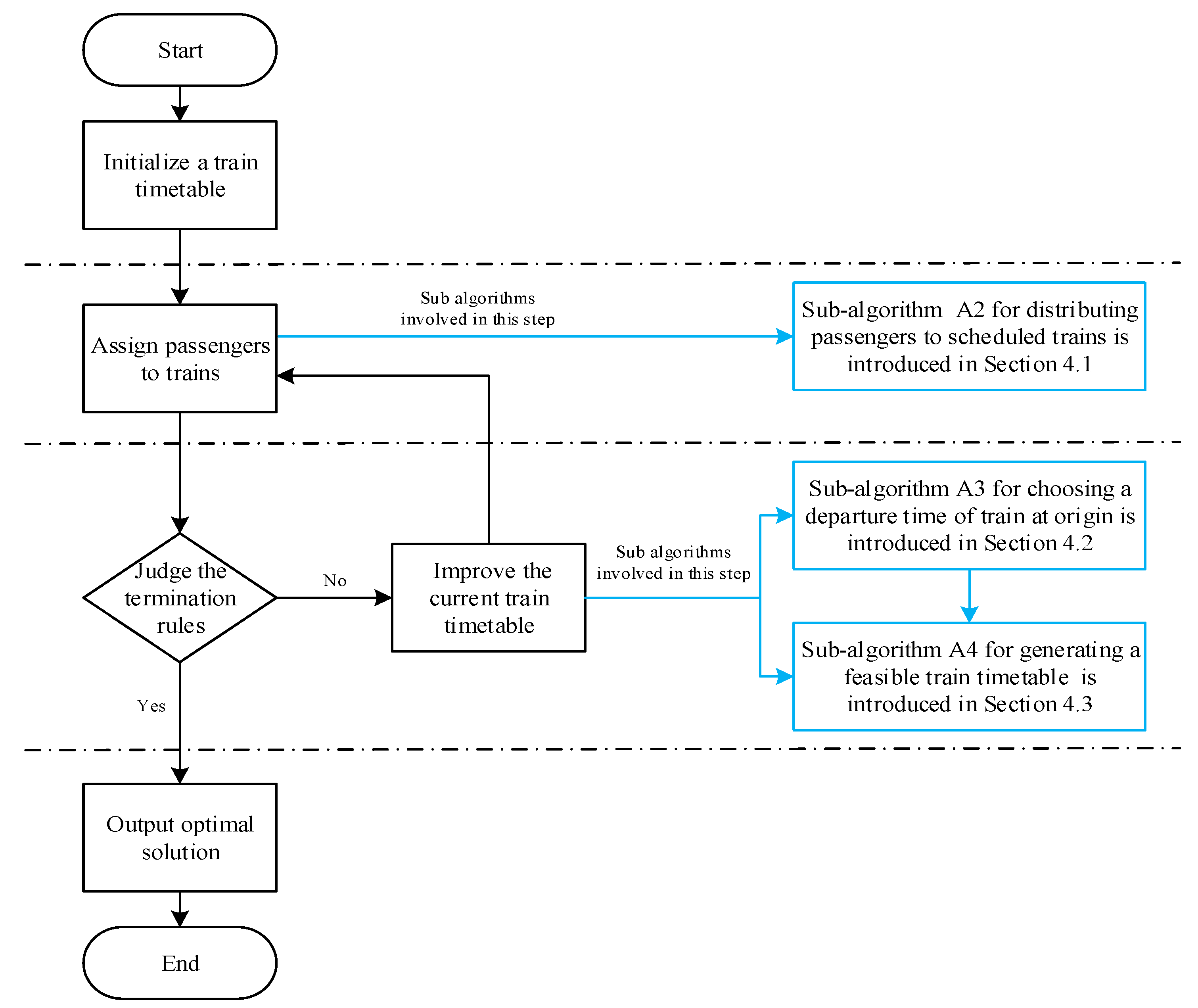
The solving procedure and the relations between the priority-based heuristic Algorithm (A1) and its sub-algorithms are shown in Figure 2:
- Initialize a train timetable. Schedule trains one by one based on a random order. Specifically, for each train, set its departure time at its origin as the middle time of the departure time range, and then compute its arrival and departure time at each visited station according to this origin departure time and train minimum travel time in sections and dwell time at stations.
- Equilibrium assignment of passenger flow. Based on the initial timetable, use a path-based passenger distribution Algorithm (A2) to assign passengers to trains, namely, to determine the number of passengers booking each train. The specific steps are illustrated in Section 4.1.
- Update criterion of the optimal solution and judge the termination rules as follows; use criteria similar to the metropolis criteria to determine whether the new solution is accepted. If , is accepted as the new current solution , otherwise is accepted as the new current solution with the probability . is the objective function, is the current solution, and is the new solution.
The following three rules are set to control the termination of the algorithm.
- The iteration count reaches its maximum value.
- The objective of model UM cannot be improved for continuous time.
- The difference in passenger costs between the last two iterations satisfieswhererepresents the set of paths chosen by demandin theth iteration, and are, respectively, the number and generalized cost of time periodfor passengers traveling on pathfrom originto destinationin theth iteration. In addition, is a given small positive number.
- Improve the current train timetable. Rearrange trains’ arrival and departure times to improve the current timetable based on the present passenger train-booking decisions and obtain a new train timetable.
In summary, the frame of the priority-based heuristic is given in Algorithm 1 (A1), and more detailed explanations for some steps and sub-algorithms are introduced afterwards.
| Algorithm 1 A priority-based heuristic Algorithm (A1) for DOTTP combining passenger train-booking decisions. |
| Input:. Output:, upper-level objective function value (UO), lower-level objective function value (LO) Rank trains based on the decreasing order of their speeds, and sort those with the same speed in descending order of their travel mileages. Trains in the front have higher priority than those in the back. For:
Assign passengers to trains based on the current train timetable using the passenger distribution Sub-Algorithm (A2) introduced in Section 4.1. While termination rules 1,2,3 detailed before this algorithm are not met:
End Assign passengers to trains based on the current train timetable using the passenger distribution Sub-Algorithm (A2) introduced in Section 4.1. End |
In the above Algorithm (A1), the initial train timetable obtained may not be feasible because train arrival and departure times may not satisfy the safety interval constraints, which are not considered. However, the improved train timetable obtained by the Sub-Algorithm (A4) must be feasible.
4.1. Sub-Algorithm (A2) for Distributing Passengers to Scheduled Trains
The Sub-Algorithm (A2) of the above priority-based heuristic Algorithm (A1) is to distribute passengers to scheduled trains. Thus, this section focuses on detailing a sub-algorithm for assigning passengers to scheduled trains. The passenger distribution methods are generally divided into link-based and path-based types. Compared with the link-based approach, the path-based method will not only provide more path information about passengers including their travel trains and each part of the cost on the paths, but also have much higher solving efficiency (see Jayakrishnan [47] and Chen [48]). Hence, we prefer to apply a path-based passenger distribution algorithm to solve model LM.
The following two notes should be emphasized before detailing Sub-Algorithm (A2).
- Update the passenger number of chosen paths and the current lowest-cost path as follows:whereandare, respectively, the first and second derivatives of objectiveto passenger number of path, andis the lowest-cost path in theth iteration. Moreover, is the updating step, andis a given fixed value. Obviously,becomes smaller with the increase of iteration. If the passenger number of chosen path is updated as 0, then we delete it from the set of chosen paths as it is not chosen by any passengers.
- The termination rules of Sub-Algorithm (A2).where is a given small tolerance value.
In summary, we detail Sub-Algorithm (A2) for distributing passengers to trains in Algorithm 2.
| Algorithm 2 Sub-Algorithm (A2) for distributing passengers to scheduled trains. |
| Input:, the current train timetable. Output:, upper-level objective function value (UO), lower-level objective function value (LO). Initialize iteration count. Search the lowest cost pathfor each granularity-based demand. Distribute all passengersto the lowest-cost path, and initialize the set of chosen paths. While the inequality in Equation (18) is not satisfied:
Calculate the upper-level objective function value (UO) and the lower-level objective function value (UO) according to Equations (1) and (9) respectively. |
4.2. Sub-Algorithm (A3) for Choosing a Departure Time of a Train at Origin
Generally, the departure time of a train at origin has a great influence on passengers’ deviation time and transferring time, but little effect on passengers’ in-vehicle time as a train’s travel time is usually only allowed to vary within a small range. For simplicity, we first determine the departure time of the train at origin with the objective of minimizing the total deviation and transferring times of its distributed passengers, and then calculate its arrival and departure times at other visited stations. Therefore, we first have to calculate the deviation and transferring times of passengers traveling partially or wholly with the current scheduling train before detailing the algorithm. The following two notes should be emphasized when calculating them.
- We do not need to calculate those deviations and transferring times that are unaffected by the current scheduling train. For instance, we do not calculate the deviation time of passengers who first board a scheduled train and then transfer to the current scheduling train as their deviation time is determined by the former train not the latter one.
- For unscheduled trains, we calculate the travel times between two stations based on their travel times in sections and minimum dwell times at stations. Especially for the current scheduling train, we can determine arrival and departure times at stations from a given departure time at origin based on its travel times in sections and minimum dwell times at stations.
Set train as the current scheduling train and denote decision variable as its departure time at origin. Then, we calculate the deviation and transferring times of passengers traveling with it in two sub-trips, respectively. The first sub-trip is before traveling with train, and the other is after traveling with train.
Passenger deviation and transferring times in their first sub-trip are calculated with the following three types of passengers, respectively:
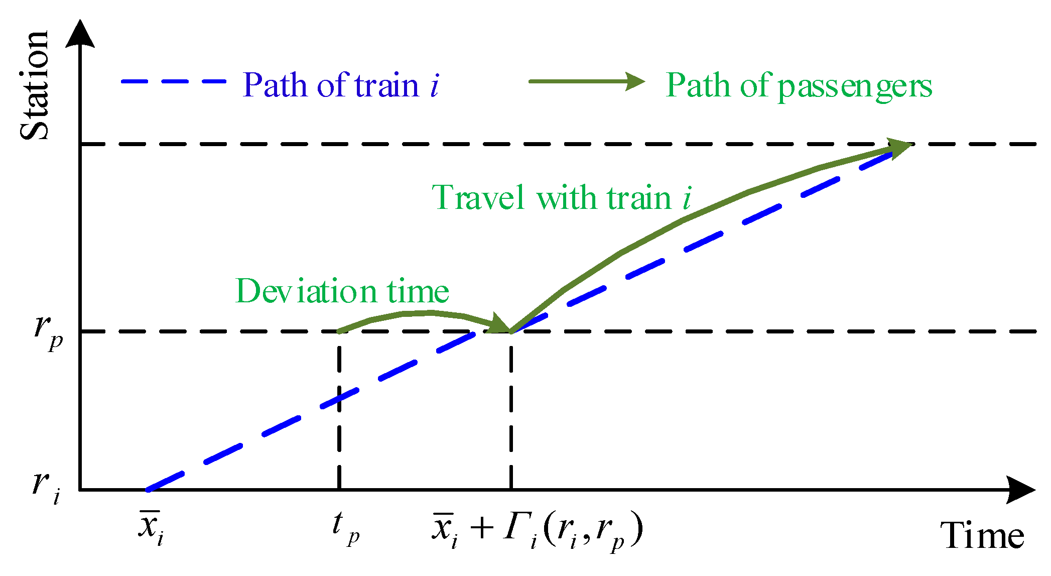
4.2.1. Type 1: Passengers Whose First Travel Train Is just Train
As illustrated in Figure 3, andare the origin stations of trainand passengers respectively, is the travel time of trainfrom stationto station, andis the planned time of passengers. For this type of passengers, their transferring time before traveling with trainis set as 0 as they don’t need to transfer, and their deviation time at origin denoted asis calculated by
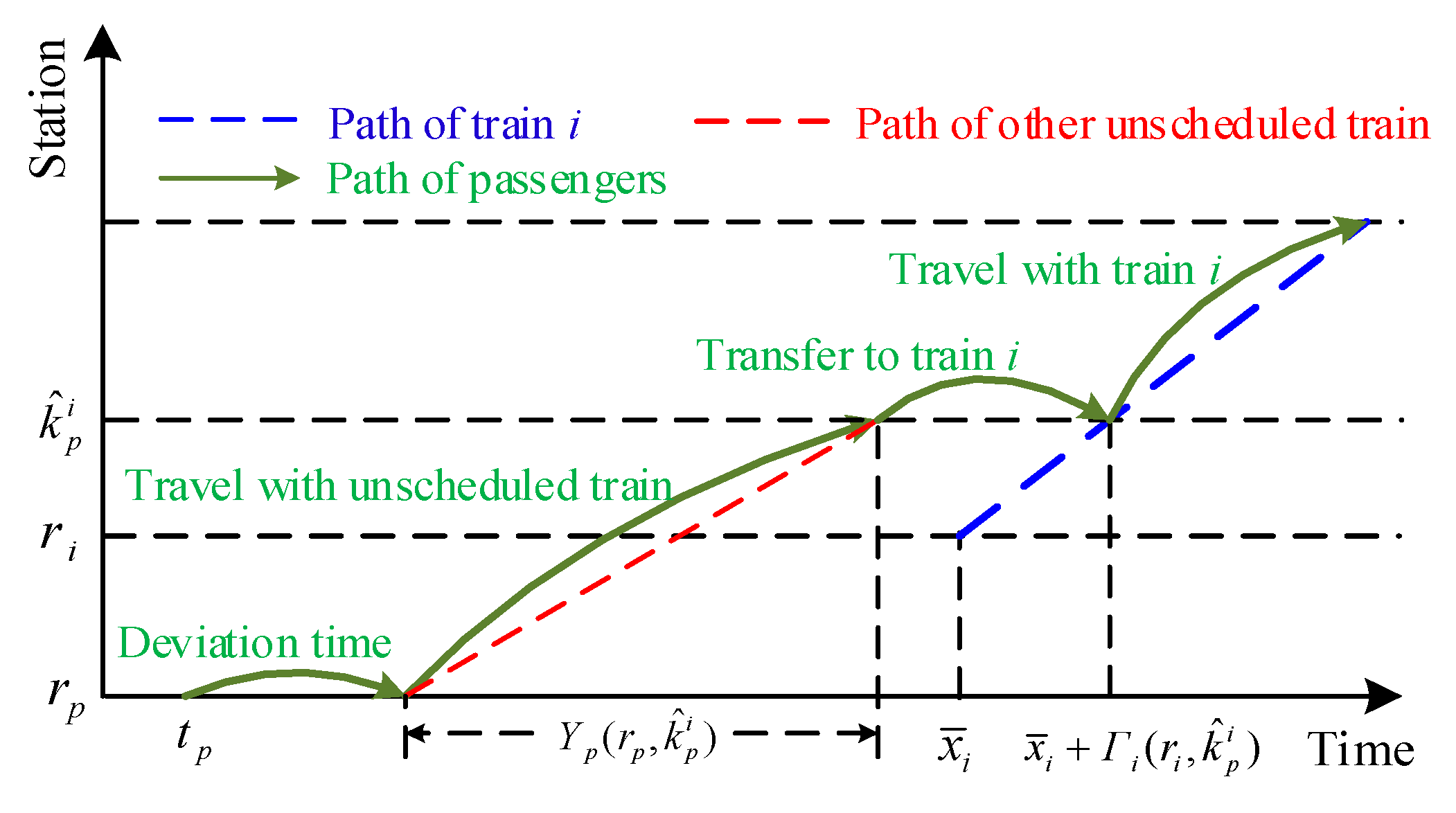
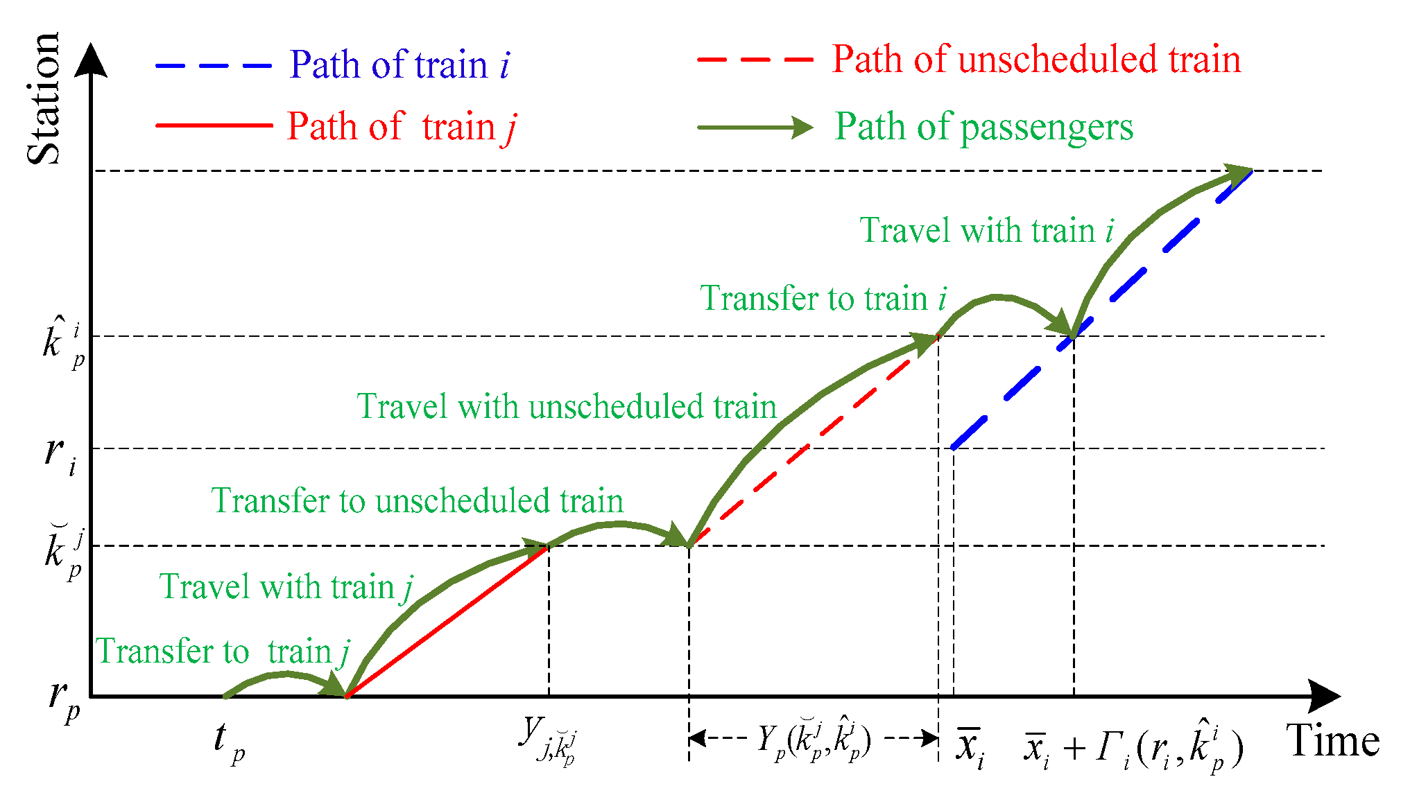
4.2.2. Type 2: Passengers Whose Traveling Trains before Train Are Unscheduled
This type of passengers has to first travel with some unscheduled trains, and then transfer to train, as shown in Figure 4, in whichis the station passengers transferring to train, and is passenger total in-vehicle time from stationto stationtraveling with one or more unscheduled trains. For this type of passengers, their transferring time before traveling with trainis set as the minimum transferring time, and their deviation time can be determined as
4.2.3. Type 3: Passengers Whose Traveling Trains Exist at least One Scheduled Train before Train
Assume trainas the last one among these scheduled trains that passengers travel with before train, as shown in Figure 5. Obviously, their deviation and transfer times before trainare irrelevant to train, and only those passengers who get off trainto get on trainare influenced by train, and their transferring times are calculated by
whererepresents passenger total transferring time before traveling with train, is the station passenger getting on train, and is set as a given big value, which can be viewed as a penalty value when passengers cannot transfer to train as it departs earlier.
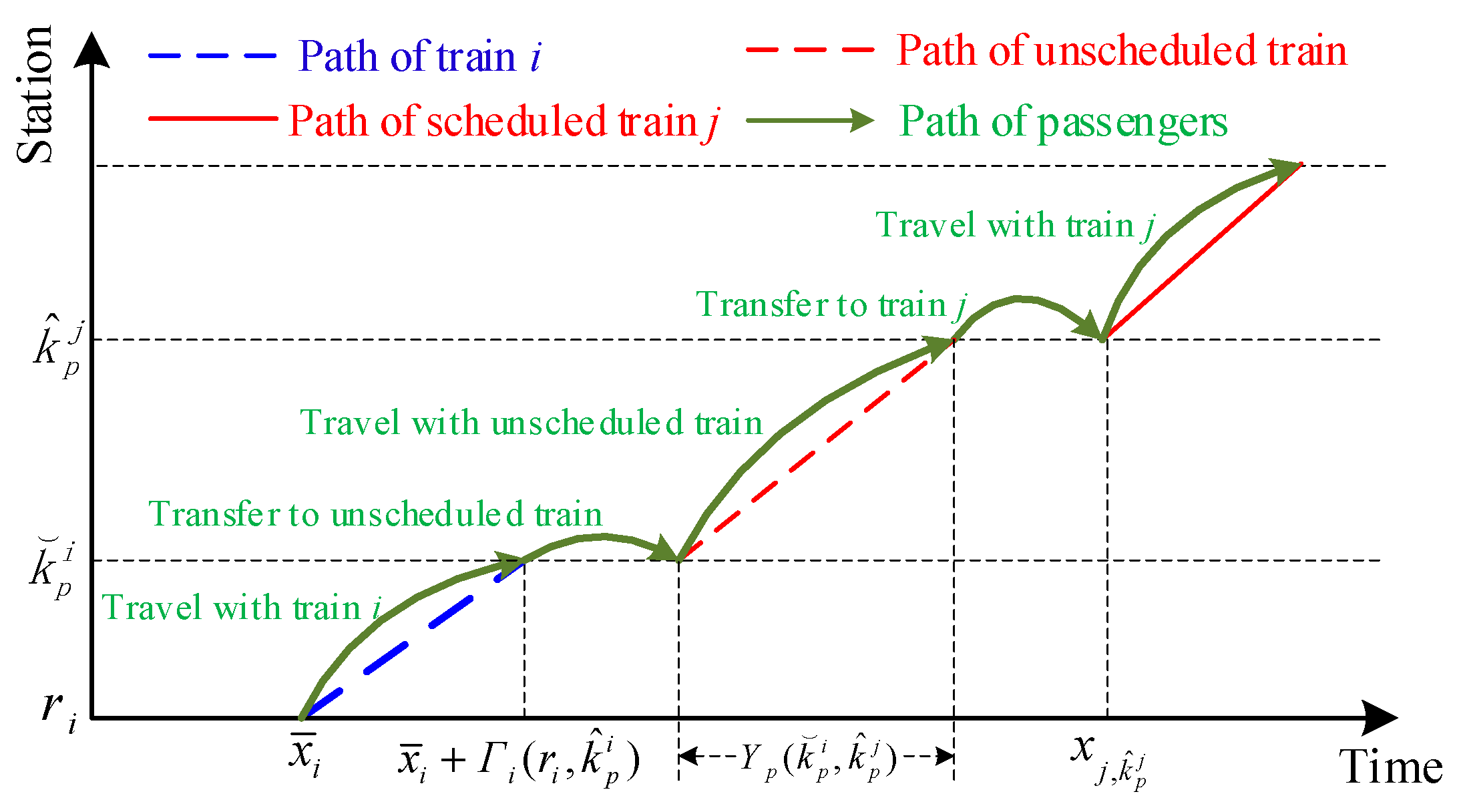
Next, we further calculate passenger transfer times in the sub-trip after train. They are set as 0 in the following two cases: (1) train is the last train passengers traveling; and (2) all traveled trains after train are not scheduled. Only when at least one scheduled train passenger traveling after train exists, as shown in Figure 6, and train is assumed as the first one among these scheduled trains passengers traveling after train, we should calculate passenger transfer time denoted asfrom getting off train to getting on train as follows:
In conclusion, the objective of choosing departure time for train at origin is described as
whereis the path set of passengers traveling with train wholly or partially, andis the passenger number on path.
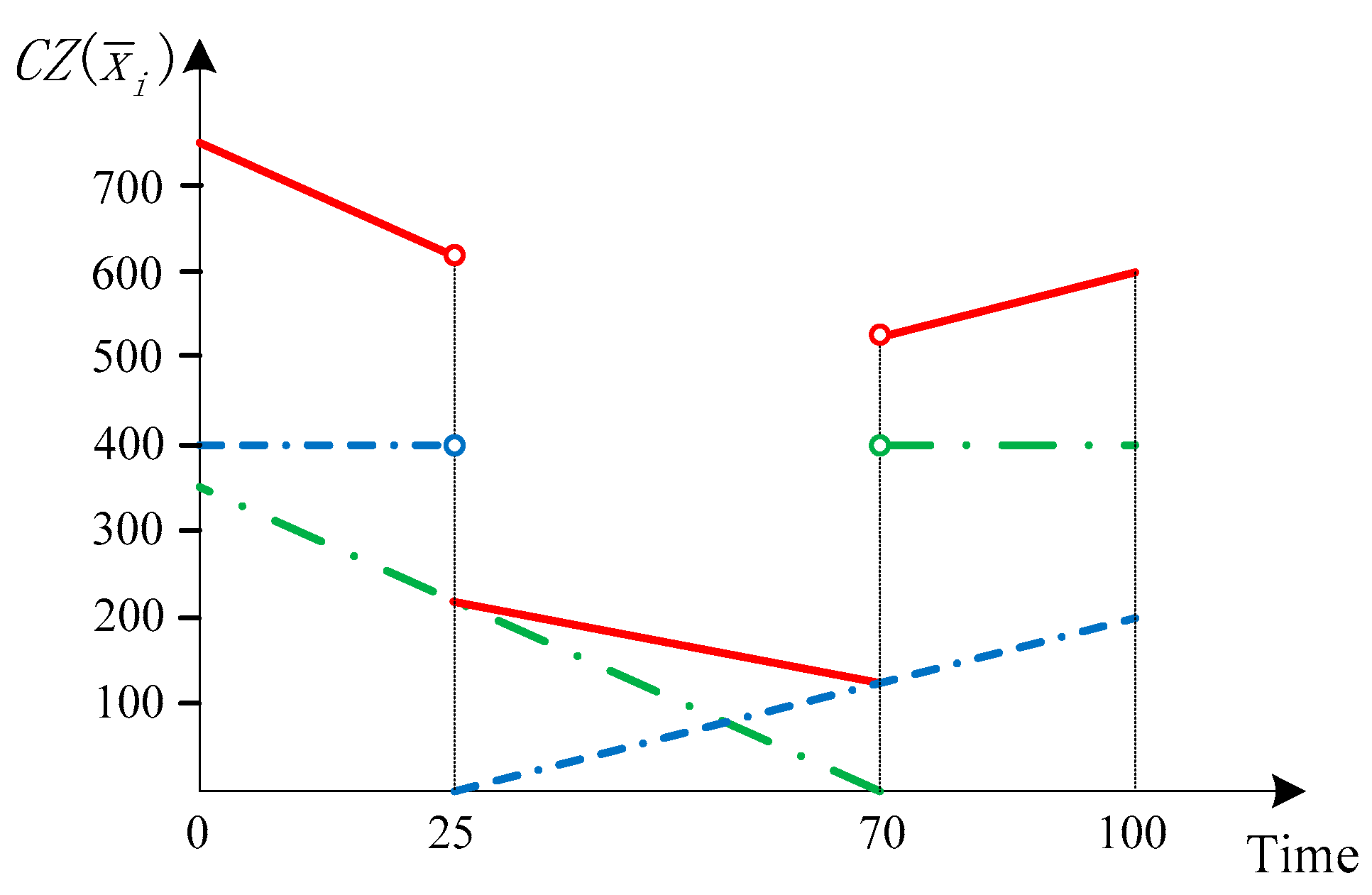
The objective functionis a piecewise linear function of train departure timeas all of its component functions in Equations (19)–(22) are piecewise and their all segments are linear. The segregating times of function are those of Equations (19)–(22). As illustrated in Figure 7, the green and blue dashed lines display two piecewise functions that form the objective function shown with red solid lines. Function is piecewise and contains three linear segments separated by time points 25 and 70 in the planning horizon from 0 to 100, and the best departure time is time point 70.
Based on the segmentation characteristics of the objective function, Algorithm (A3), intended to choose the departure time at origin for train, is shown in Algorithm 3.
| Algorithm 3 Sub-Algorithm (A3) for choosing the departure time at origin for train. |
| Input:, the current train timetable. Output: a set of departure time of trainat origin. Find passenger paths consisting of train, and determine the segregating times from the calculation of Equations (19)–(23) of deviation and transferring times on them. Sort all segregating times as well as departure times of all scheduled trains at the origin station of train, and then divide the planning horizon into multiple time segments using them as splitting times. Find the optimal time for each time segment, and then rank them based on the increasing order of their corresponding values of. Choose the best, next best, or other required time as the departure time of train at origin. |
In Step 3 of Sub-Algorithm (A3), we can easily determine the optimal time of each time segment according to the continuous and monotonic function. That is, if increases with time, then the optimal departure time is determined as the left border of this segment; otherwise, it is chosen as the right one.
4.3. Sub-Algorithm (A4) for Generating a Feasible Train Timetable Based on Given Departure Times
As train arrival and departure times calculated in Algorithm (A1) may not satisfy safety interval requirements, this subsection focuses on making them satisfy these requirements through finely adjusting them with the aid of a weighted directed graph. Their adjustment must obey the follows rules.
- It is not permitted to generate new conflicts. A conflict represents the condition that two involved trains do not satisfy the safety interval.
- The increment of passengers’ deviation time should be limited to a given small range, but its decrement is welcome. For example, a train departing at 10:10 before adjustment has been chosen by passengers of time 10:00, and then its departure time is only allowed to adjust in the range from 10:00 to 10:15 as 5 min is set as the maximum increment of passengers’ deviation time. Similarly, the increments of passenger transfer time and dwell times at stations also must be limited to a small range.
Before detailing this algorithm, we first build a weighted directed graph corresponding to the train timetable as follows:
4.3.1. Nodes of Graph
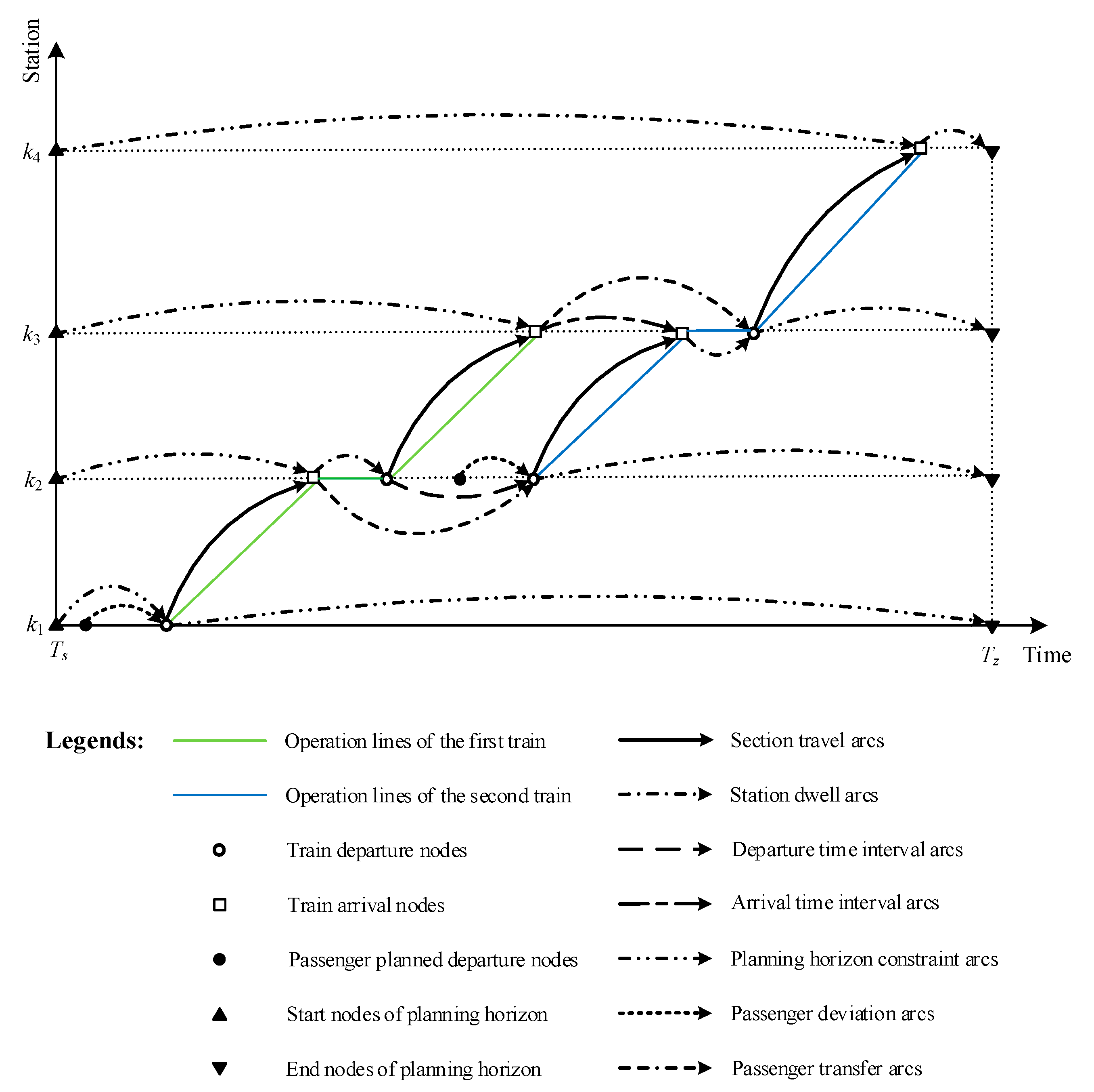
Five types of nodes are defined in Table 4.
It should be noted that the start and end nodes of the planning horizon are defined for each station, and, thus, their numbers are just the number of stations. A weight is defined for each node, and εν is denoted as the weight of node ν. Moreover, only the weights of train departure and arrival nodes can be adjusted while other nodes are not allowed to be adjusted.
4.3.2. Directed Arcs of the Graph
Seven types of directed arcs are constructed between nodes shown in Figure 8 to restrict the adjustment of train arrival and departure times, and their detailed definitions, requirements, and weights are introduced in Table 5.
Takeas the weight of directed arc andas its minimum and maximum values, respectively. The weight of each arc should range between its minimum and maximum.
In the construction process of directed arcs, the following four notes should be emphasized:
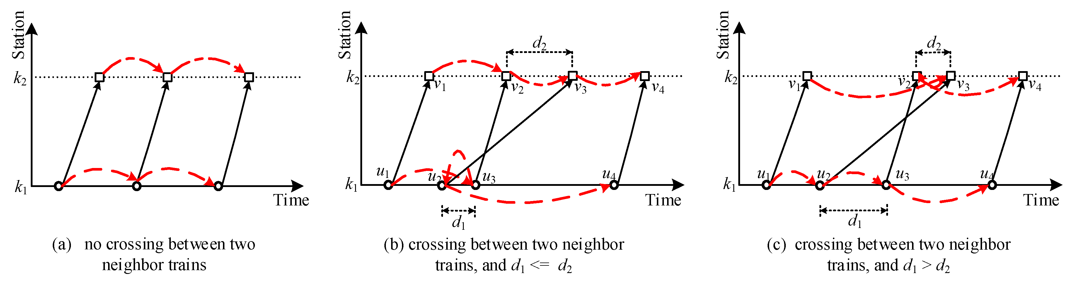
- As the number of departure (arrival) time interval arcs is very large when they are constructed between any two trains’ departure (arrival) nodes of the same station, we only construct these between two neighbor trains’ departure (arrival) nodes as shown with the red dotted lines in Figure 9a for reducing their number. However, if two trains cross in a section, then their interval arcs are constructed in two cases, as shown with the red dotted lines in Figure 9b,c, respectively.
- Similarly, planning horizon constraint arcs are only defined for the first and last trains’ departure or arrival nodes at a station for reducing their number.
- For passenger deviation and transfer arcs, they are constructed only when there are passengers traveling from their start nodes to their terminal nodes. For example, if passengers are boarding Train 1 rather than Train 2 at their origin, then we should construct the passenger deviation arc from these passengers’ departure node to the departure node of Train 1, not to that of Train 2 as they do not board it.
- The maximum increments of passenger dwell time, deviation time, and transfer time are pre-specified as inputs of the algorithm. Generally, the smaller they are, the smaller the increase of passenger travel time, and the higher the difficulty of obtaining a feasible train timetable is. Thus, we can set them as smaller values at first when the number of trains is considerably below the capacity of the rail line, namely, the maximum of scheduled trains on the rail line, and then gradually increase them as the train numbers increase.
Now, with the help of the weighted directed graph of the train timetable, we introduce how to finely adjust train arrival and departure times to make them satisfy all constraints of model UM.
First, we find the set of all conflict arcs whose weights are less than their minimum weights and denote them as. According to the construction method of the initial train timetable given in Algorithm (A1), we ensure that all section travel arcs, station dwell arcs, passenger deviation, and transfer arcs satisfy their minimum and maximum weight requirements, and only the departure time interval arcs, arrival time interval arcs, and planning horizon constraint arcs may become conflict arcs.
Second, we increase the weights of conflict arcs one by one. For the conflict arc, its weight can be increased by either reducing the weight of node or increasing the weight of node. Denoteand as the sets of associate adjusted nodes when adjusting the weights of nodes and, respectively. Specifically, we only decrease the weights of nodes in setsimultaneously for reducing the weight of node, and similarly only increase the weights of nodes in setsynchronously to add the weight of node. For example, as illustrated in Figure 10a, we can increase the weight of the conflict arcshown with the red dotted line by reducing the weight of nodeand increasing the weight of node, and setis determined asshown with the blue color because the weight of the dwell arcis less than its maximum value 2, while setis decided asshown in the green color.
The detailed steps of searching setare given in Algorithm 4, and steps for setare similar.
| Algorithm 4 The detailed steps for searching set. |
| Input: conflict arcs, the weighted directed graph,. Output: . Initialize set. For : Find all outbound arcsand all inbound arcs for node. For : If : Add nodeinto set. For : If : Add nodeinto set. End |
The maximum weight decrementof node setis calculated by
and the maximum weight increment of the node setis determined as
Then, their actual adjustments are determined separately by
According to them, we can update the weights of nodes in setandas follows.
Correspondingly, the weights of arcs whose start or end nodes belong to setorare updated as follows.
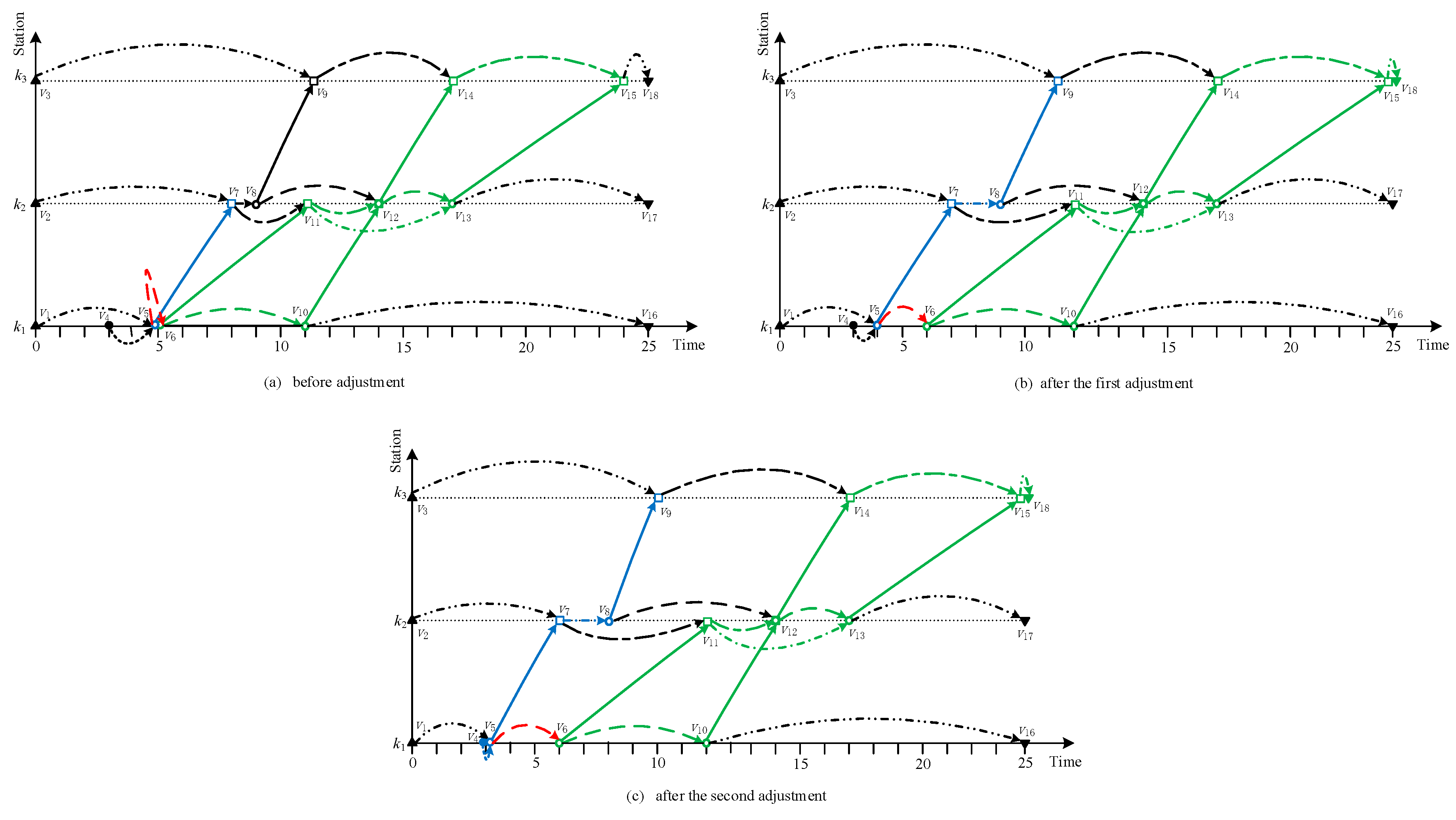
For example, both the maximum weight decrement and incrementare 1 in Figure 10a, and their actual adjustments are also determined as 1. After updating the weights of all relevant nodes and arcs, we can obtain the weighted directed graph as shown in Figure 10b. If we want to further reduce the weight of node, we should add nodesandinto setto simultaneously adjust for the weight of dwell arcreaching its maximum. Similarly, if we continue to increase the weight of node, we still have to add node into set.
After the above adjustment of node and arc weights, if conflict arcsatisfies, then stop and choose another conflict arc to adjust its weight; otherwise, update setsand, and repeat the above adjustment process of weights.
In the adjustment process of weights, if setcontains a node whose weight is not allowed to be changed, then we cannot decrease the weights of nodes in setany further. Similarly, if setincludes a constant-weight node, then we cannot further increase the weights of nodes in set. Therefore, if the weights of both nodes in setsandcannot be further adjusted and the weightof the conflict arcis still less than its minimum, it means that we cannot obtain a feasible train timetable from the initial train timetable. In this case, we have to construct another initial train timetable based on a new departure time and adopt the proposed algorithm in this subsection again to find a feasible train timetable. For instance, we cannot further increase the node weights of setin Figure 10b as it contains node, so we only continue to decrease the node weights of setto further increase the weight of conflict arc, and then update the weighted directed graph, as shown in Figure 10c, in which the weight of the arcreaches its minimum value of three, and its corresponding train timetable is feasible.
In summary, the steps of Sub-Algorithm (A4) for making train departure and arrival times feasible from an initial train timetable are detailed in Algorithm 5.
| Algorithm 5 Sub-Algorithm (A4) for forming a feasible train timetable based on given departure times. |
| Input: the current train timetable,. Output: a feasible train timetable. Generate the weighted directed graph based on the given initial train timetable. Find the conflict arc set, fixed nodes set. While:
|
5. Numerical Analysis
To test the validity of our method, this section takes the Changsha–Zhuzhou–Xiangtan intercity rail network to test our proposed approach, and analyzes its performance, convergence and effectiveness based on the obtained optimization results.
5.1. Inputs and Parameter Setting
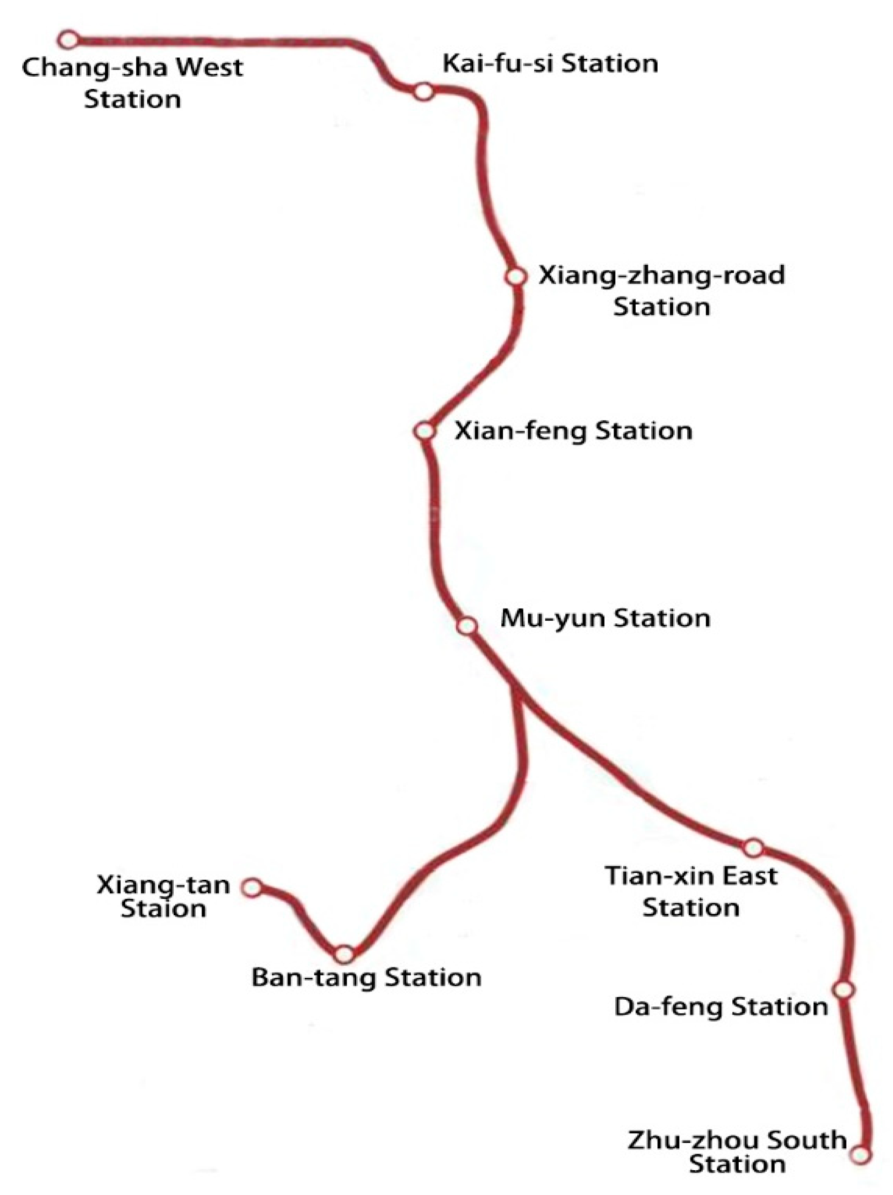
The Changsha–Zhuzhou–Xiangtan (CZT) intercity railway network consists of 24 stations, of which 23 stations are in operation now, as shown in Figure 11. It has the mileage of 104.36 km, and provides fast, punctual and convenient transportation services among Changsha, Zhuzhou and Xiangtan cities. About 80% of passengers on this network are recently distributed among the ten busiest stations, including Chang-sha West, Xian-feng, Ban-tang, Xiang-tan, and Tian-xin East. For simplicity, we retain only these stations with many departures and arrivals, and remove those with fewer passengers visiting in CZT rail network to construct a “Y”-shaped test network consisting of 10 stations and 9 sections to test our proposed method.
As all sections have two one-way tracks in our test network, the numerical example only focuses on scheduling trains from Changsha to Zhuzhou, or Changsha to Xiangtan. The stations visited by trains of the two paths are shown in Table 6.
The actual operation time of CZT intercity rail network now is from 07:00 to 23:00, and it is also applied as our optimization time horizon of trains. Currently, there are 43 trains operating in this time horizon, of which 22 trains are bounded from Chang-sha West Station to Zhu-zhou South station, and 21 trains are bounded from Chang-sha West to Xiang-tan station. More detailed information can be obtained from the website: www.12306.com [49]. Obviously, these operating trains and the volume of service passengers are small, and are far less than the service capacity of this network. For better testing our method, we operate the corresponding number of passenger trains based on the predicted number of passengers sent out in 2020 (see Shao [50] and Pan [51]). Therefore, there are 100 trains operating all day, of which 60 trains are from Chang-sha West station to Zhu-zhou South station and 40 trains are from Chang-sha West station to Xiang-tan station. The parameters of operating trains on two paths are shown in Table 7.
In the whole rail network, there are 39 pairs of OD passenger flows in total. The passengers’ origin station, terminal station, and demand quantity of each OD pair are shown in Table 8.
Taking five minutes as unit time interval, the operating time of whole day can be divided into 192 time periods; each pair of OD passenger flow is assigned to the corresponding time period. Suppose the passengers’ travelling ratio coefficient of every time period in morning rush hours (7:00–9:00) and evening rush hours (17:00–19:00) are 0.0084, while that of every time period in other non-peak hours is 0.0041. The minimum safety departure interval and minimum safety arrival interval in various transit sections are set as 3 min, and the other parameters for the algorithm are set as shown in Table 9.
The above two algorithms were both solved by MATLAB 2016a, using the hardware of a Lenovo C5030 desktop computer corresponding to 2 GHz Intel (TM) Core (TM) i3-5005U CPU, 8 GB (4) memory, and Windows 10 specialized operating system.
5.2. Convergence Analysis
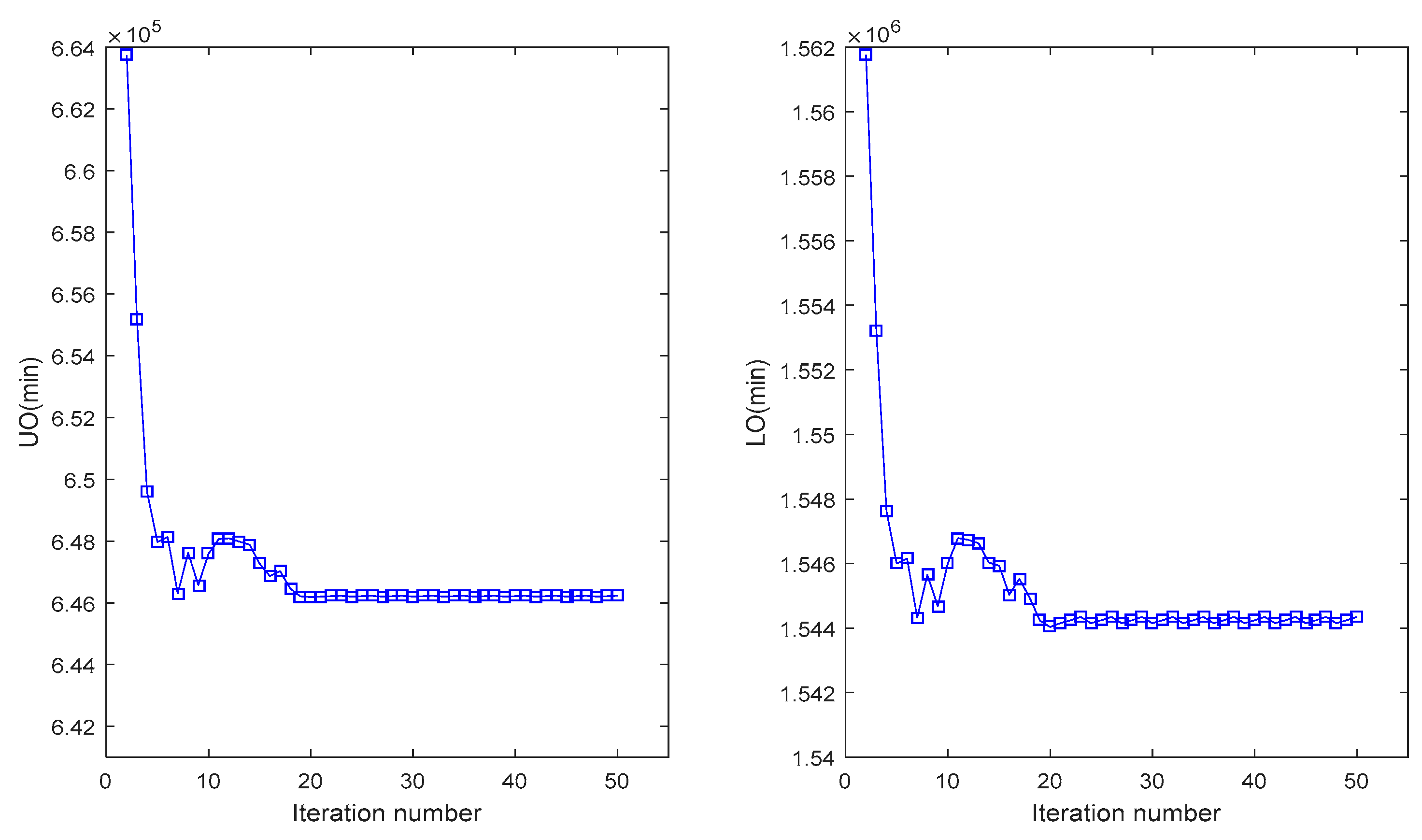
Figure 12 (left) shows the change of upper-level objective function value (UO) along with the increasing number of iterations in the proposed algorithm, while the change of lower-level objective function value (LO) is shown in Figure 12 (right).
Figure 12 demonstrates that, with the continuous increase of the iteration number, the objective function value UO and LO decrease rapidly at first, and then decrease slowly until the algorithm converges smoothly. In the convergence process of UO, the number of iterations needed for the algorithm to reach convergence is about 50, but, in fact, the convergence solution was obtained in 20 iterations. It indicates that our proposed algorithm performs well in convergence.
5.3. Equilibrium Analysis
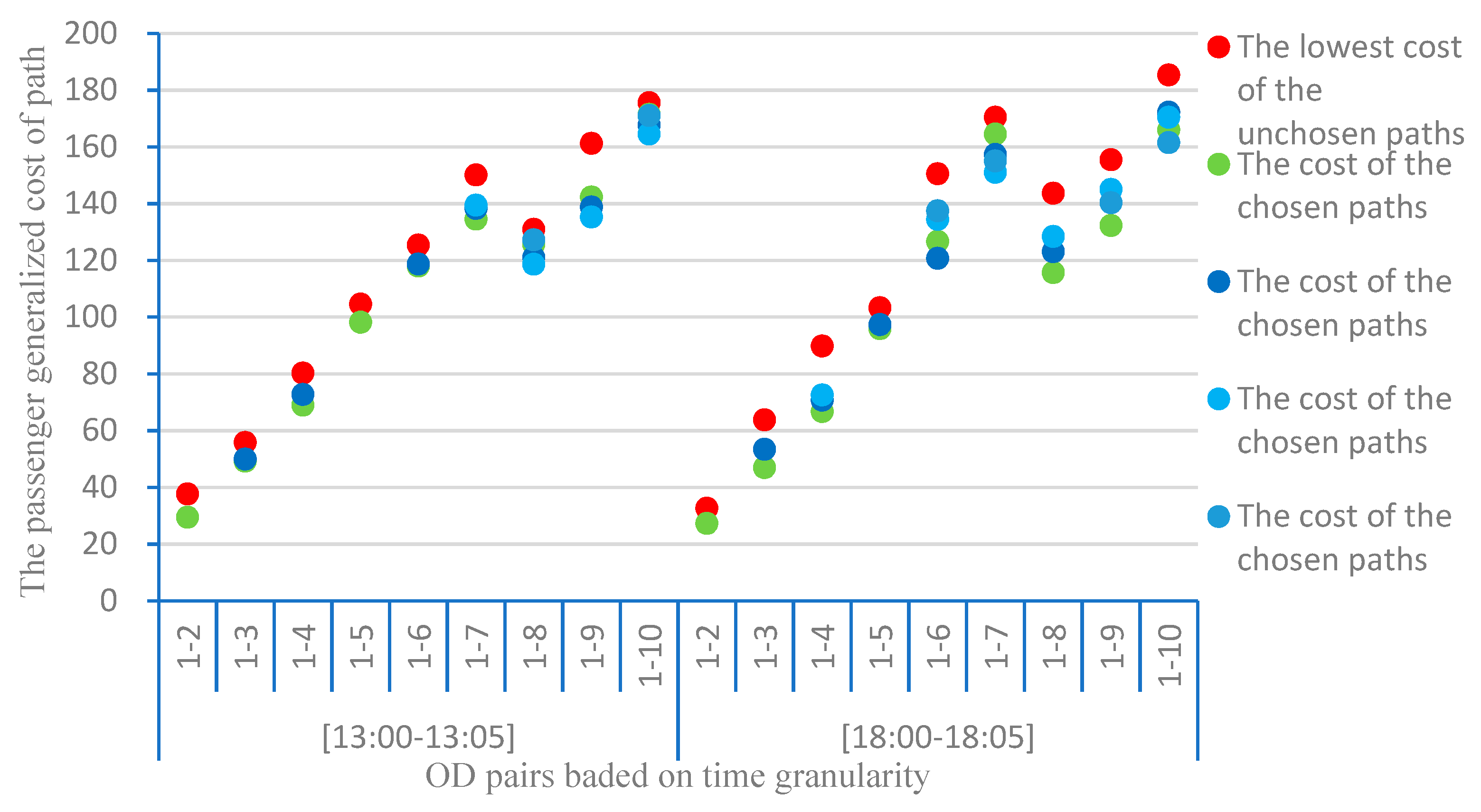
To judge whether the OD passenger flow distribution in each time-period has reached an equilibrium, this section aims to analyze the behaviors of passengers’ train-booking in the optimized results obtained by our proposed algorithm. Due to the huge number of granularity-based demands, it is hard to enumerate their chosen paths in detail one by one, thus we only select the optimized results of path-choice in two time periods (13:00–13:05 and 18:00–18:05) as examples to assess the effect of passengers assignment. The paths chosen or not chosen by passengers and its passenger generalized cost are shown in Figure 13.
Figure 13 shows that the passengers of each OD-pair can choose at least one path to travel, and the generalized travel cost on their chosen paths are almost equivalent with each other. Furthermore, for every OD-pair, the generalized travel cost on chosen paths (green dots, dark blue dots, light blue dots, and cyan dots) are all less than the minimum among other unchosen paths (red dots). Therefore, it proves that the passenger assignment has achieved an equilibrium. For example, doe OD 1–8 in time period 13:00–13:05, the total number of passengers corresponding to this OD is 20, and they are assigned to four different paths with the number of passengers being 5, 5, 3 and 7, respectively. The relevant generalized travel cost on these four paths are accordingly 125.65, 121.00, 118.60 and 127.25. It is obvious that the difference among them are limited in a small range, and all of them are no more than the minimum among other paths not chosen by passengers of this OD-pair.
5.4. The Benefits of Scheduling Trains Considering Passenger Train-Choosing
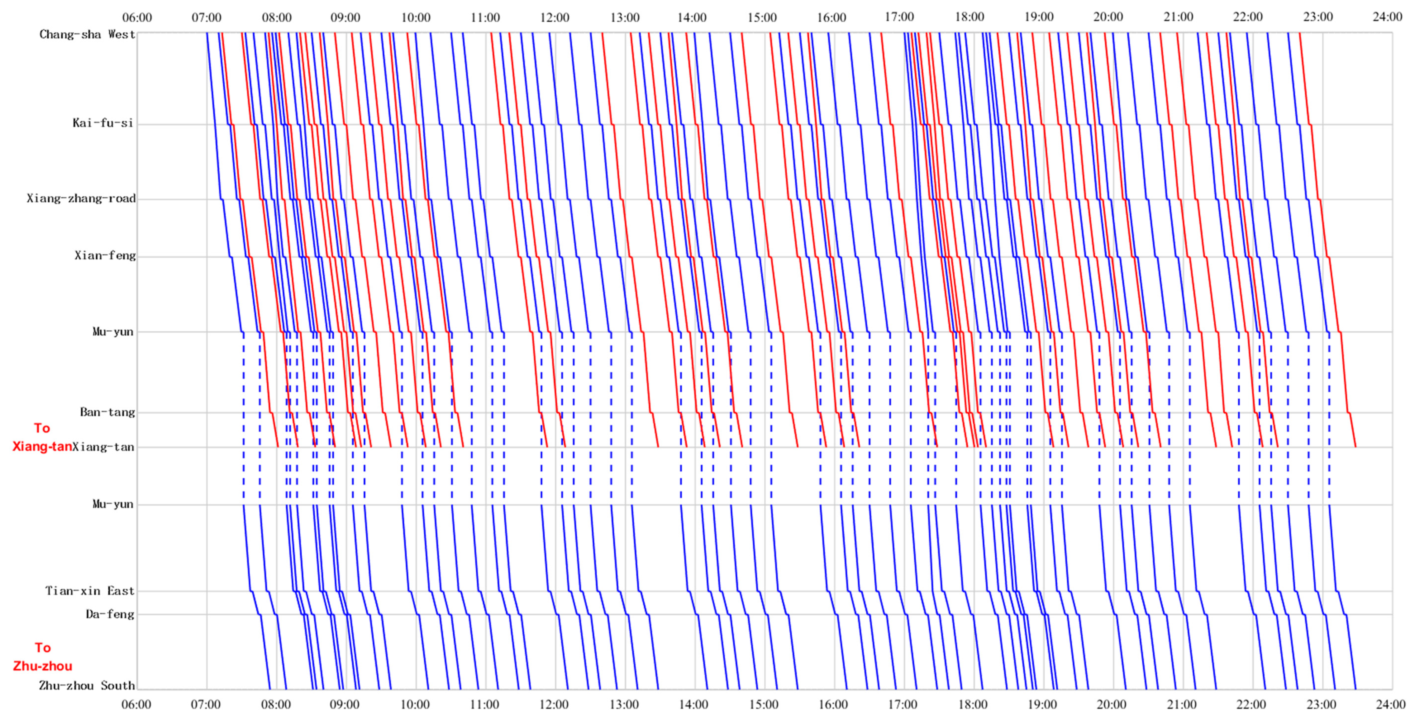
To show the benefits of scheduling trains integrating passenger train-choosing, this section first optimizes train schedules with the above input using a passenger-free algorithm, and then optimizes it with our proposed algorithm. By comparing these results obtained by two algorithms, respectively, we analyze the benefits of our algorithm regarding with passenger service level. Note that our algorithm optimizes the train timetable combining with passenger’ train-booking, while passenger-free algorithm only schedules trains by minimizing the summation of train travel time subject to some operation headway constraints, and the service level of the train timetable obtained by the latter is determined by distributing passengers to trains at last. Figure 14 gives the train diagram optimized by our proposed algorithm. Table 10 gives the objectives, the average deviation times of passengers at origins and the average travel speeds of two algorithms.
Table 10 demonstrates that values of indicators in our proposed algorithm are obviously better than those obtained in the passenger-free algorithm. On the one hand, per capita deviation time of passengers in our algorithm is reduced by 29.86% compared to that in passenger-free algorithm, which is because we have taken train-booking of passengers into account so that making optimized timetable is well matched with the actual passenger trip rules. On the other hand, as the stop plan was optimized in our algorithm, per capita travelling speed is increased by 10.34% compared with that in passenger-free algorithm.
To illustrate the performance of two algorithms specifically, more indicators are presented to evaluate and analyze comparatively between two algorithms.
5.4.1. Average Travel Speed of Each OD Pairs
Based on the results shown in Figure 15, the average travel speed of each OD passenger flow in our algorithm is significantly faster than that in passenger-free algorithm. Specifically, in our algorithm, the average travel speed is 104.35 km/h, while it is 93.57 km/h in the passenger-free algorithm. Moreover, the percent of OD pairs whose average travel speed exceeds 100 km/h is 53.85% in our algorithm compared with only 20.51% in passenger-free algorithm. Thus, the train schedule obtained by our algorithm can give passengers a much faster travel speed, which improves the travel efficiency of passengers in urban region and ensures the timeliness of travel.
5.4.2. Percentage of Passengers Corresponding to Different Deviation Time at Origin
As illustrated in Table 11, the train timetable obtained by the algorithm in this paper can significantly reduce the deviation time of passengers at the origin station through detailed data. Specifically, the percentage of passengers in our algorithm are all higher than passenger-free algorithm when their deviation time is shorter than 15 min, while they are all lower than passenger-free algorithm when their deviation time is longer than 15 min. For example, on the train timetable obtained by our algorithm, 47.35% of the passengers have a deviation time of less than 5 min at origin, compared with 39.98%. Similarly, the former only has 3.58% of passengers whose deviation time is more than 30 min at origin, while the latter is 12.95%.
5.4.3. The Changing Trend of Passengers’ Demand and Running Trains’ Number
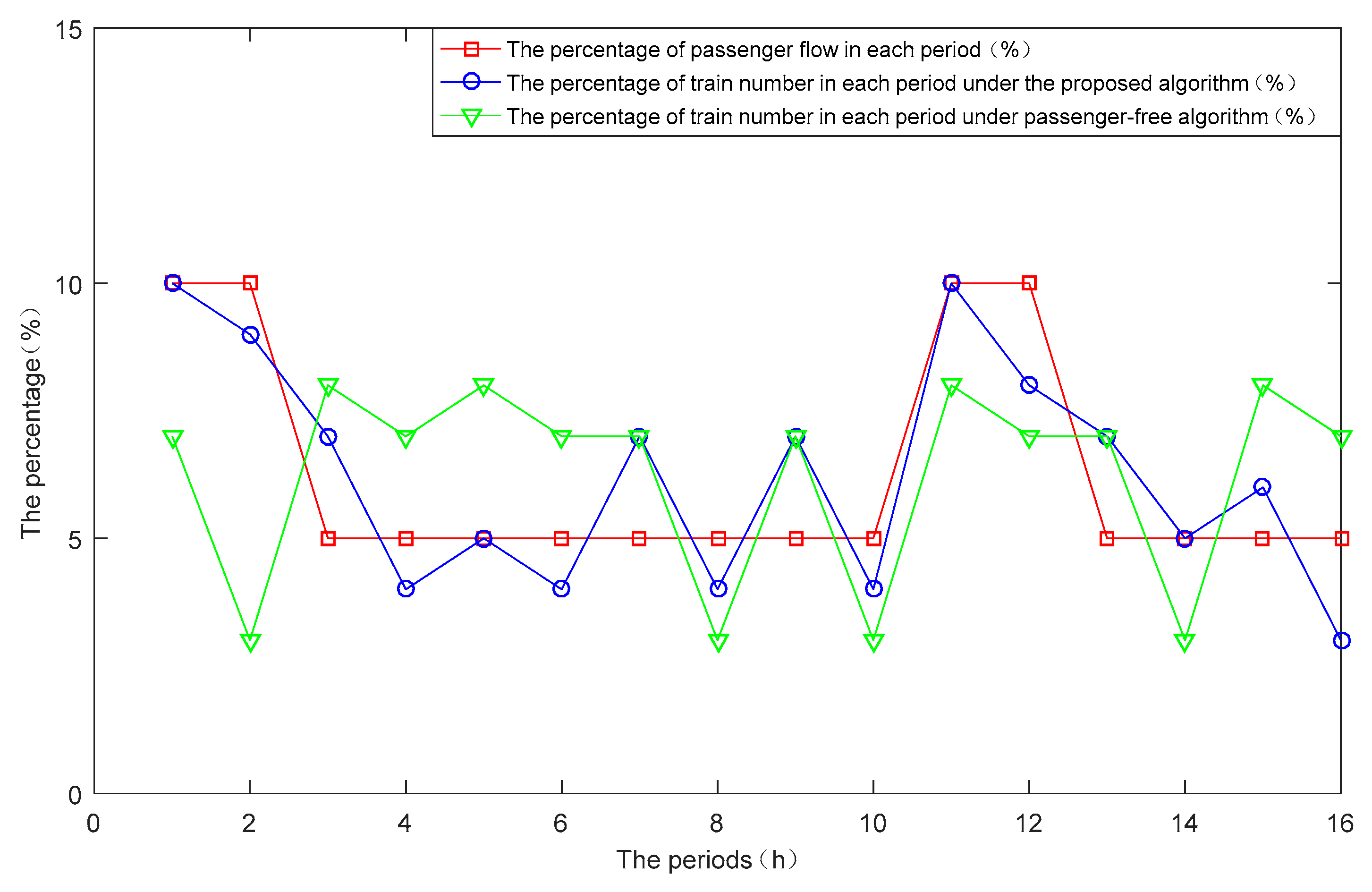
To analyze the matching degree between train capacity and passenger flow in different periods, their matching curves are presented in Figure 16. Due to the huge number of granularity-based demands, we integrate data in units of 1 h. The red line denotes the percentage of passenger flow in each period, while the blue and green lines represent the percentage of train number in each period optimized by our proposed algorithm and passenger-free algorithm, respectively. According to the changing trend of three lines, we can draw the conclusion that the changing trend of train number is more consistent with passenger travel demand in our algorithm, while there is no obvious matching relationship in passenger-free algorithm.
5.4.4. Service Frequency of Each OD Pair
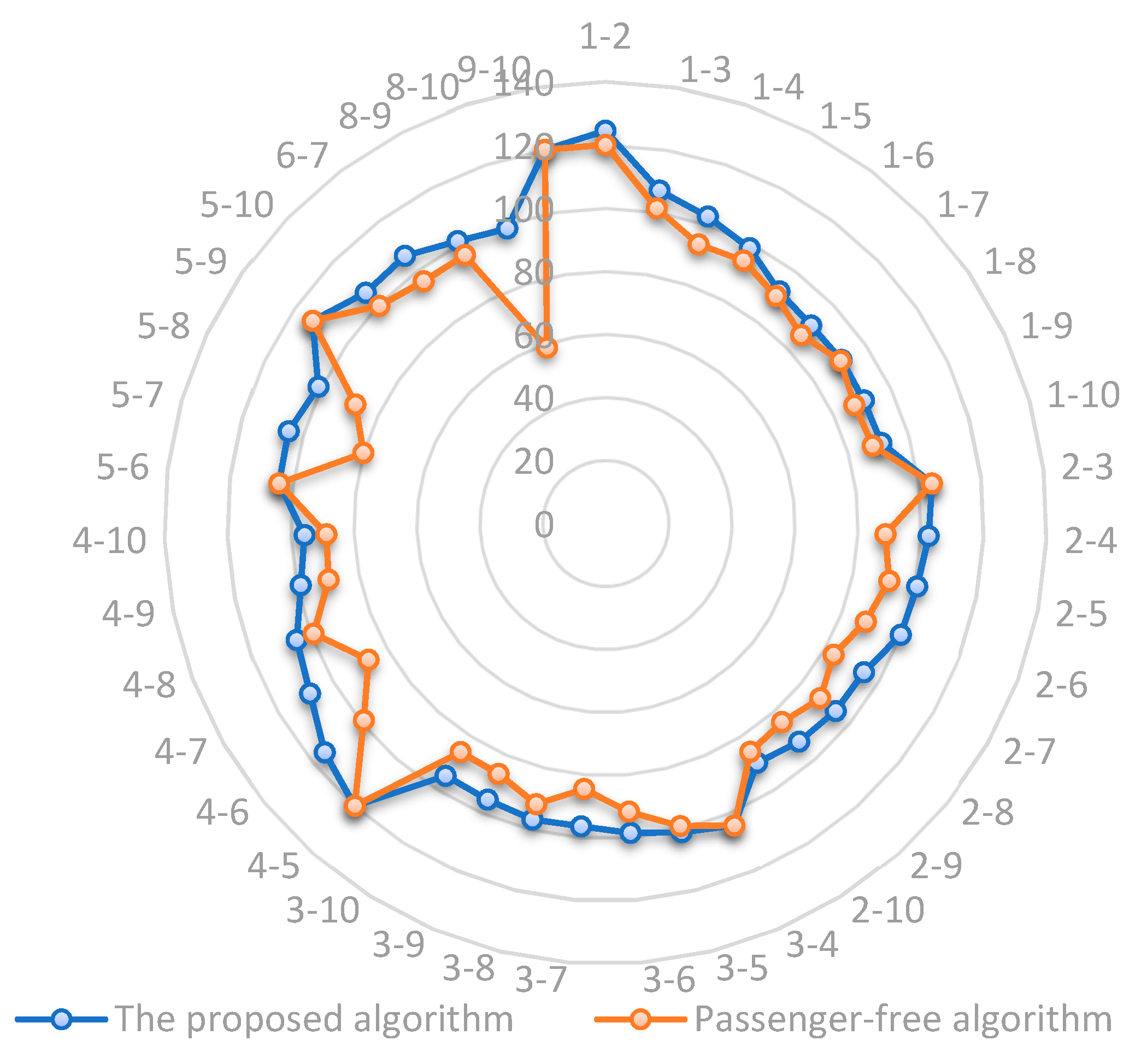
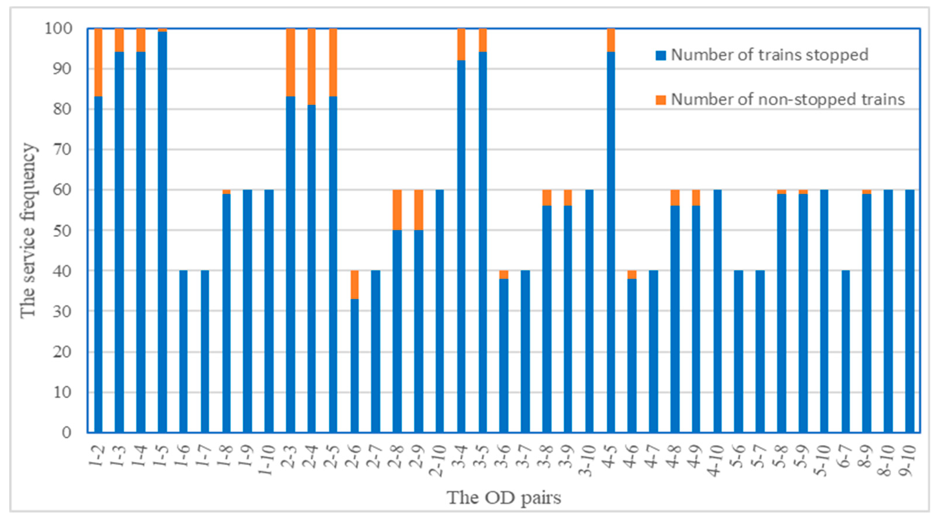
A satisfactory train schedule should not only minimize the total travel time and travel cost of passengers, but also optimize the service frequency between OD pairs along the railway line. In the process of optimizing the arrival and departure times at stations of trains, our algorithm also takes the optimization of train stops into consideration. On the train schedule obtained by our algorithm, the service frequency of each OD pair of CZT Intercity Railway is shown in Figure 17. As shown in Figure 16, the service frequency of each OD pair effectively match with its travel demand, so that trains’ total travel time is cut down, and the satisfaction of passengers is improved greatly.
6. Conclusions and Further Study
To apply the feedback of passenger train-booking decisions to guide the optimization of the demand-oriented train timetable, this paper combines passengers’ equilibrium assignment to trains into train timetable optimization and proposes a priority-based heuristic approach for demand-oriented train timetabling. The train timetable obtained by the proposed method has a higher service level. It can reduce the travel cost of passengers, thereby attract more passengers to choose the more energy-efficient and environmentally friendly railway and actively promote the sustainable development of society. The main conclusions of this paper are as follows:
- A bi-level programming model is designed for a demand-oriented train timetabling problem integrated with the train-booking decisions of passengers, and a priority-based heuristic algorithm is designed to solve this model. The proposed algorithm consists of three sub-algorithms for distributing passengers to trains, finding trains’ original departure times based on their priorities and distributed passengers, and generating a feasible train timetable, respectively.
- Experimental results from the Changsha–Zhuzhou–Xiangtan intercity rail network show that the train timetable obtained by our proposed method has higher service level compared with that of a passenger-free algorithm. On the one hand, the per capita deviation time of passengers in our algorithm is reduced by 29.86% compared to that in the passenger-free algorithm, and the per capita traveling speed is increased by 10.34% compared with that in the passenger-free algorithm. On the other hand, as the train stop plan was optimized in our algorithm, the number of train stops is reduced by 6.11%, which reduces the energy consumption and time waste caused by the stops. Moreover, the optimized train timetable is well-matched with the actual passenger trip rules, which effectively improves the load factor of the trains.
The following are worth further study in the future.
- In this paper, each station is simplified as a node with parking capacity, but the train’s travel path at a station is not considered. Therefore, future studies should consider combining the train routing problem at stations with the train timetabling problem to obtain a more practical train timetable.
- Due to the competition between expressways and intercity railways, the service level of the train timetable has a great influence on its passenger demand. Thus, it is necessary to optimize the train schedule further considering the elastic change relationship between passenger demand and train service level.
Author Contributions
W.Z. and W.F. conceived the study, established the models and designed the algorithm; W.F. achieved the program code and conducted the data experiments; W.F. and X.Y. were responsible for data analysis and editing; W.Z. and W.F. wrote the paper; and W.Z., X.Y. and L.D. helped to modify the paper.
Funding
This research work was partially supported by the National Natural Science Foundation of China (Grant Nos. 71871226, 71401182, and 71471179), the Natural Science Foundation of Hunan Province, China (Grant No. 2018JJ3698), and the Fundament Research Funds for the Central Universities of Central South University (Grant No. 2019zzts545). The authors are responsible for all results and opinions expressed in this paper.
Acknowledgments
The authors would like to acknowledge the anonymous reviewers for their valuable comments.
Conflicts of Interest
The authors declare no conflict of interest. The funders had no role in the design of the study; in the collection, analyses, or interpretation of data; in the writing of the manuscript, or in the decision to publish the results.
References
- Higgins, A.; Kozan, E.; Ferreira, L. Optimal scheduling of trains on a single line track. Transp. Res. Part B Methodol. 1996, 30, 147–161. [Google Scholar] [CrossRef] [Green Version]
- Burdett, R.; Kozan, E. A disjunctive graph model and framework for constructing new train schedules. Eur. J. Oper. Res. 2010, 200, 85–98. [Google Scholar] [CrossRef]
- Zhou, W.; Teng, H. Simultaneous passenger train routing and timetabling using an efficient train-based Lagrangian relaxation decomposition. Transp. Res. Part B Methodol. 2016, 94, 409–439. [Google Scholar] [CrossRef]
- Bešinović, N.; Goverde, R.M.; Quaglietta, E.; Roberti, R. An integrated micro–macro approach to robust railway timetabling. Transp. Res. Part B Methodol. 2016, 87, 14–32. [Google Scholar]
- Zhou, W.; Tian, J.; Xue, L.; Jiang, M.; Deng, L.; Qin, J. Multi-periodic train timetabling using a period-type-based lagrangian relaxation decomposition. Transp. Res. Part B Methodol. 2017, 105, 144–173. [Google Scholar] [CrossRef]
- Goverde, R.M.P. Railway timetable stability analysis using max-plus system theory. Transp. Res. Part B Methodol. 2007, 41, 179–201. [Google Scholar] [CrossRef]
- Corman, F.; D’Ariano, A.; Pacciarelli, D.; Pranzo, M. Bi-objective conflict detection and resolution in railway traffic management. Transp. Res. Part C Emerg. Technol. 2012, 20, 79–94. [Google Scholar] [CrossRef]
- Xu, X.; Li, K.; Yang, L.; Ye, J. Balanced train timetabling on a single-line railway with optimized velocity. Appl. Math. Model. 2014, 38, 894–909. [Google Scholar] [CrossRef]
- Brannlund, U.; Lindberg, P.O.; Nou, A.; Nilsson, J.E. Railway timetabling using lagrangian relaxation. Transp. Sci. 1998, 32, 358–369. [Google Scholar] [CrossRef]
- Robenek, T.; Maknoon, Y.; Azadeh, S.S.; Chen, J.; Bierlaire, M. Passenger centric train timetabling problem. Transp. Res. Part B 2016, 89, 107–126. [Google Scholar] [CrossRef] [Green Version]
- Li, X.; Wang, D.; Li, K.; Gao, Z. A green train scheduling model and fuzzy multi-objective optimization algorithm. Appl. Math. Model. 2013, 37, 2063–2073. [Google Scholar]
- Carey, M.; Crawford, I. Scheduling trains on a network of busy complex stations. Transp. Res. Part B Methodol. 2007, 41, 159–178. [Google Scholar] [CrossRef]
- Caimi, G.; Chudak, F.; Fuchsberger, M.; Laumanns, M.; Zenklusen, R. A new resource-constrained multicommodity flow model for conflict-free train routing and scheduling. Transp. Sci. 2011, 45, 212–227. [Google Scholar] [CrossRef]
- Dundar, S.; Şahin, İ. Train re-scheduling with genetic algorithms and artificial neural networks for single-track railways. Transp. Res. Part C Emerg. Technol. 2013, 27, 1–15. [Google Scholar] [CrossRef]
- Marguier, P.H.J.; Ceder, A. Passenger waiting strategies for overlapping bus routes. Transp. Sci. 1984, 18, 207–230. [Google Scholar] [CrossRef]
- Herbon, A.; Hadas, Y. Determining optimal frequency and vehicle capacity for public transit routes: A generalized newsvendor model. Transp. Res. Part B Methodol. 2015, 71, 85–99. [Google Scholar] [CrossRef]
- Yang, X.; Li, X.; Gao, Z.; Wang, H.; Tang, T. A cooperative scheduling model for timetable optimization in subway systems. IEEE Trans. Intell. Transp. Syst. 2013, 14, 438–447. [Google Scholar] [CrossRef]
- Zheng, Y.J.; Ling, H.F.; Shi, H.H.; Chen, H.S.; Chen, S.Y. Emergency railway wagon scheduling by hybrid biogeography-based optimization. Comput. Oper. Res. 2014, 43, 1–8. [Google Scholar] [CrossRef]
- Dobson, G.; Lederer, P.J. Airline Scheduling and Routing in a Hub-and-Spoke System. Transp. Sci. 1993, 27, 281–297. [Google Scholar] [CrossRef]
- Jiang, H.; Barnhart, C. Dynamic airline scheduling. Transp. Sci. 2009, 43, 336–354. [Google Scholar] [CrossRef]
- Parbo, J.; Anker Nielsen, O.; Giacomo Prato, C. Passenger perspectives in railway timetabling: A literature review. Transp. Rev. 2016, 36, 500–526. [Google Scholar] [CrossRef]
- Yu, B.; Yang, Z.; Yao, J. Genetic algorithm for bus frequency optimization. J. Transp. Eng. 2010, 136, 576–583. [Google Scholar] [CrossRef]
- Ma, T.Y. A Hybrid Multiagent Learning Algorithm for Solving the Dynamic Simulation-Based Continuous Transit Network Design Problem. In Proceedings of the International Conference on Technologies & Applications of Artificial Intelligence, Chung-Li, Taiwan, 11–13 November 2012. [Google Scholar]
- Wang, J.Y.; Lin, C.M. Mass transit route network design using genetic algorithm. J. Chin. Inst. Eng. 2010, 33, 301–315. [Google Scholar] [CrossRef]
- Cordone, R.; Redaelli, F. Optimizing the demand captured by a railway system with a regular timetable. Transp. Res. Part B Methodol. 2011, 45, 430–446. [Google Scholar] [CrossRef]
- Parbo, J.; Nielsen, O.A.; Prato, C.G. User perspectives in public transport timetable optimisation. Transp. Res. Part C Emerg. Technol. 2014, 48, 269–284. [Google Scholar] [CrossRef] [Green Version]
- Kaspi, M.; Raviv, T. Service-Oriented Line Planning and Timetabling for Passenger Trains. Transp. Sci. 2013, 47, 295–311. [Google Scholar] [CrossRef]
- Canca, D.; Barrena, E.; De-Los-Santos, A.; Andrade-Pineda, J.L. Setting lines frequency and capacity in dense railway rapid transit networks with simultaneous passenger assignment. Transp. Res. Part B 2016, 93, 251–267. [Google Scholar] [CrossRef]
- Yang, X.; Chen, A.; Ning, B.; Tang, T. Bi-objective programming approach for solving the metro timetable optimization problem with dwell time uncertainty. Transp. Res. Part E 2017, 97, 22–37. [Google Scholar] [CrossRef]
- Barrena, E.; Canca, D.; Coelho, L.C.; Laporte, G. Exact formulations and algorithm for the train timetabling problem with dynamic demand. Comput. Oper. Res. 2014, 44, 66–74. [Google Scholar] [CrossRef]
- Niu, H.; Zhou, X.; Gao, R. Train scheduling for minimizing passenger waiting time with time-dependent demand and skip-stop patterns: Nonlinear integer programming models with linear constraints. Transp. Res. Part B Methodol. 2015, 76, 117–135. [Google Scholar] [CrossRef]
- Yang, L.; Zhang, Y.; Li, S.; Gao, Y. A two-stage stochastic optimization model for the transfer activity choice in metro networks. Transp. Res. Part B Methodol. 2016, 83, 271–297. [Google Scholar] [CrossRef]
- Johan, H.; Markus, B.; Oskar, F. A combined simulation-optimization approach for minimizing travel time and delays in railway timetables. Transp. Res. Part B Methodol. 2019, 126, 192–212. [Google Scholar]
- Zhang, T.; Li, D.; Qiao, Y. Comprehensive optimization of urban rail transit timetable by minimizing total travel times under time-dependent passenger demand and congested conditions. Appl. Math. Model. 2018, 58, 421–446. [Google Scholar] [CrossRef]
- Ibarra-Rojas, O.J.; Giesen, R.; Rios-Solis, Y.A. An integrated approach for timetabling and vehicle scheduling problems to analyze the trade-off between level of service and operating costs of transit networks. Transp. Res. Part B Methodol. 2014, 70, 35–46. [Google Scholar] [CrossRef]
- Liu, T.; Ceder, A. Integrated public transport timetable synchronization and vehicle scheduling with demand assignment: A bi-objective bi-level model using deficit function approach. Transp. Res. Procedia 2017, 23, 341–361. [Google Scholar] [CrossRef]
- Liu, T.; Ceder, A.; Chowdhury, S. Integrated public transport timetable synchronization with vehicle scheduling. Transp. A Transp. Sci. 2017, 6, 1–23. [Google Scholar] [CrossRef]
- Wang, H.; Jiang, Z.; Zhang, H.; Wang, Y.; Yang, Y.; Li, Y. An integrated MCDM approach considering demands-matching for reverse logistics. J. Clean. Prod. 2019, 208, 199–210. [Google Scholar] [CrossRef]
- Abdelghany, A.; Abdelghany, K.; Azadian, F. Airline flight schedule planning under competition. Comput. Oper. Res. 2017, 87, 20–39. [Google Scholar] [CrossRef]
- Niu, H.; Zhou, X. Optimizing urban rail timetable under time-dependent demand and oversaturated conditions. Transp. Res. Part C Emerg. Technol. 2013, 36, 212–230. [Google Scholar] [CrossRef]
- Wang, Y.; Tang, T.; Ning, B.; van den Boom, T.J.; Schutter, B. De Passenger-demands-oriented train scheduling for an urban rail transit network. Transp. Res. Part C 2015, 60, 1–23. [Google Scholar] [CrossRef]
- Wang, Y.; D’Ariano, A.; Yin, J.; Meng, L.; Tang, T.; Ning, B. Passenger demand oriented train scheduling and rolling stock circulation planning for an urban rail transit line. Transp. Res. Part B Methodol. 2018, 118, 193–227. [Google Scholar] [CrossRef]
- Shi, J.; Yang, L.; Yang, J.; Gao, Z. Service-oriented train timetabling with collaborative passenger flow control on an oversaturated metro line: An integer linear optimizatin approach. Transp. Res. Part. B Methodol. 2018, 110, 26–59. [Google Scholar] [CrossRef]
- Fu, H.; Nie, L.; Meng, L.; Sperry, B.R.; He, Z. A hierarchical line planning approach for a large-scale high speed rail network: The china case. Transp. Res. Part A 2015, 75, 61–83. [Google Scholar] [CrossRef]
- Mahmassani, H.S.; Chen, S.T. An investigation of the reliability of real-time information for route choice decisions in a congested traffic system. Transportation 1993, 20, 157–178. [Google Scholar] [CrossRef]
- Watling, D. User equilibrium traffic network assignment with stochastic travel times and late arrival penalty. Eur. J. Oper. Res. 2006, 175, 1539–1556. [Google Scholar] [CrossRef] [Green Version]
- Jayakrishnan, R.; Mahmassani, H.S.; Hu, T.Y. An evaluation tool for advanced traffic information and management systems in urban networks. Transp. Res. Part C Emerg. Technol. 1994, 2, 129–147. [Google Scholar] [CrossRef]
- Chen, A.; Lee, D.H.; Jayakrishnan, R. Computational study of state-of-the-art path-based traffic assignment algorithms. Math. Comput. Simul. 2002, 59, 509–518. [Google Scholar] [CrossRef]
- 12306 China Railway. Available online: www.12306.com (accessed on 15 March 2019).
- Shao, M. Study on Passenger Flow Forecast and Transportation Organization of the Chang Chu Tan Intercity Railway. Ph.D. Thesis, Southwest Jiaotong University, Chengdu, China, 2015. [Google Scholar]
- Pan, D. Forecast of Passenger Flow for Chang-Zhu-Tan Intercity Rail Transit. Ph.D. Thesis, Changsha University of Science & Technology, Changsha, China, 2012. [Google Scholar]
Figure 1.
Leader–follower relationship of decision-making between rail enterprises and passengers.

Figure 2.
The flowchart of the priority-based heuristic Algorithm (A1).

Figure 3.
A trip example of the first type of passengers.

Figure 4.
A trip example of the second type of passengers.

Figure 5.
A trip example of the third type of passengers.

Figure 6.
An example of passenger partial trip after train i.

Figure 7.
An example of the piecewise objective function.

Figure 8.
The definitions of nodes and arcs in an example weighted directed graph.

Figure 9.
The construction of interval arcs in different cases.

Figure 10.
An example of increasing the weight of a conflict arc.

Figure 11.
Changsha–Zhuzhou–Xiangtan intercity rail network.

Figure 12.
The relationship between UO/LO and the number of iterations.

Figure 13.
The paths chosen or not chosen by passengers and its passenger generalized cost.

Figure 14.
The full-day train diagram of Changsha–Zhuzhou–Xiangtan Intercity Railway obtained by our algorithm.
Figure 14.
The full-day train diagram of Changsha–Zhuzhou–Xiangtan Intercity Railway obtained by our algorithm.

Figure 15.
Comparison diagram of the OD pairs’ average travel speed between two algorithms.

Figure 16.
Matching curves between train number and passenger flow in different periods.

Figure 17.
The service frequency of each OD pair in the operation period under our algorithm.


Table 1.
All symbols for expressing the input and the output of demand-oriented train timetabling problem (DOTTP).
Table 1.
All symbols for expressing the input and the output of demand-oriented train timetabling problem (DOTTP).
| Objects | Symbols | Defining Ranges | Descriptions |
|---|---|---|---|
| Rail network | The set of origin stations | ||
| The set of destination stations | |||
| The time granularities which are obtained by dividing the planning horizon into equivalent time intervals | |||
| The median time of time period | |||
| The start times of the planning horizon | |||
| The end times of the planning horizon | |||
| Trains | The set of trains | ||
| The set of travel sections of train | |||
| The set of visited stations of train | |||
| The continuous riding segment from stationto stationtraveling with train on path. Specifically, passengers are serviced by only one train in a continuous riding segment | |||
| The continuous riding segment that passengers transfer from trainto trainat stationon path | |||
| The continuous riding segment from origin to stationtraveling with train on path | |||
| The pure running time of trainin section | |||
| The additional time for starting of trainin section | |||
| The additional time for stopping of trainin section | |||
| The safety departure interval between two trains driving into sections and respectively from station | |||
| The safety arrival interval between two trains arriving at stationfrom sections andrespectively | |||
| The rated passenger capacity of train | |||
| Passengers | The passenger demand from originto destination in time period | ||
| The set of paths chosen by demand. For each path, it not only specifies the sequence of stations passengers traversing, but also assigns a specific train for the passengers to take between two neighbor stations. | |||
| The sequence of continuous riding segments of path | |||
| The discomfort penalty on trainfrom station to station | |||
| The total number of passengers getting on and off trainat station | |||
| The number of passengers on trainfrom station to station | |||
| The number of passengers boarding trainat origin in time period | |||
| The number of passengers transferring from trainto trainat station | |||
| The minimum required time for passengers to get on and off trainat stationwhen their total numbers is | |||
| Others | A parameter for adjusting the penalty level | ||
| The mileage from stationto station | |||
| The passenger price rate per mileage | |||
| The passenger average time value |
Table 2.
The definitions of the outputs (decision variables) of DOTTP.
| Symbols | Defining Ranges | Descriptions |
|---|---|---|
| 0-1 binary variable, if trainstops at station, then; otherwise,. has a similar definition with | ||
| The departure time of trainat station | ||
| The arrival time of trainat station | ||
| The passenger number of demandtraveling with path |
Table 3.
An example of train minimum dwell time with different passenger number at stations.
| Number of Passengers Getting on and off the Train | Minimum Dwell Time of Train/Seconds |
|---|---|
| <100 | 45 |
| 100–200 | 60 |
| 200–300 | 75 |
| >300 | 105–120 |
Table 4.
The definition of nodes.
| Name | Weight | Whether the Weight Can Be Changed |
|---|---|---|
| Train departure node | Corresponding train departure time | Yes |
| Train arrival node | Corresponding train arrival time | Yes |
| Passenger planned departure node | Planned departure time of the corresponding passengers | No |
| Start node of planning horizon | Start time of planning horizon | No |
| End node of planning horizon | End time of planning horizon | No |
Table 5.
The definition of directed arcs.
| Name | Start Node | Terminal Node | Requirements | Minimum Weight | Maximum Weight |
|---|---|---|---|---|---|
| Section travel arc | Train departure node | Train arrival node | Start and terminal nodes belong to a same train and section | The sum of train pure running time and additional times for starting and stopping | The sum of train pure running time and additional times for starting and stopping |
| Station dwell arc | Train arrival node | Train departure node | Start and terminal nodes belong to a same train and station | Minimum time for passenger getting on and off train | Passenger maximum allowed dwell time at a station |
| Departure time interval arc | Train departure node | Train departure node | Start and terminal nodes belong to two different trains but to a same station | Safety headway between two train departures | Positive infinity |
| Arrival time interval arc | Train arrival node | Train arrival node | Start and terminal nodes belong to two different trains but to a same station | Safety headway between two train arrivals | Positive infinity |
| Planning horizon constraint arc | Start node of planning horizon | Train arrival or departure node | Start and terminal nodes belong to a same station | 0 | Time length of planning horizon |
| Train arrival or departure node | End node of planning horizon | Start and terminal nodes belong to a same station | 0 | Time length of planning horizon | |
| Passenger deviation arc | Passenger planned departure node | Train departure node | Start and terminal nodes belong a same station | 0 | Passenger maximum allowed deviation time at origin |
| Passenger transfer arc | Train arrival node | Train departure node | Start and terminal nodes belong to two different trains but to a same station | Minimum time for transferring including times for getting off one train, boarding another train and walk between them | Passenger maximum allowed time per transfer |
Table 6.
Stations passed by two paths of CZT intercity.
| Path of Trains | Number of Stations | Sequence of Vistied Stations |
|---|---|---|
| Changsha to Zhuzhou | 8 | (1) Chang-sha West Station; (2) Kai-fu-si Station; (3) Xiang-zhang-road Station; (4) Xian-feng Station; (5) Mu-yun Station; (8) Tian-xin East Station; (9) Da-feng Station; (10) Zhu-zhou South Station |
| Changsha to Xiangtan | 7 | (1) Chang-sha West Station; (2) Kai-fu-si Station; (3) Xiang-zhang-road Station; (4) Xian-feng Station; (5) Mu-yun Station; (6) Ban-tang station; (7) Xiang-tan Station |
Table 7.
Operation parameters of Changsha–Zhuzhou–Xiangtan intercity railway.
| Paths | Number of Stations | Paths Mileage (km) | Train Number | Train Capacity | Technical Velocity (km/h) |
|---|---|---|---|---|---|
| Changsha to Zhuzhou | 8 | 86 | 60 | 1000 | 160 |
| Changsha to Xiangtan | 7 | 70 | 40 | 1000 | 160 |
Table 8.
Travel demand quantity of each OD pair.
| OD Sequence Number | Origin–Terminal Station | Passenger Volume | OD Sequence Number | Origin–Terminal Station | Passenger Volume |
|---|---|---|---|---|---|
| O-D 1 | 1–2 | 1200 | O-D 21 | 3–7 | 1200 |
| O-D 2 | 1–3 | 3600 | O-D 22 | 3–8 | 1200 |
| O-D 3 | 1–4 | 4800 | O-D 23 | 3–9 | 2400 |
| O-D 4 | 1–5 | 1200 | O-D 24 | 3–10 | 2400 |
| O-D 5 | 1–6 | 4800 | O-D 25 | 4–5 | 1200 |
| O-D 6 | 1–7 | 6000 | O-D 26 | 4–6 | 2400 |
| O-D 7 | 1–8 | 4800 | O-D 27 | 4–7 | 3600 |
| O-D 8 | 1–9 | 3600 | O-D 28 | 4–8 | 2400 |
| O-D 9 | 1–10 | 6000 | O-D 29 | 4–9 | 2400 |
| O-D 10 | 2–3 | 1200 | O-D 30 | 4–10 | 3600 |
| O-D 11 | 2–4 | 2400 | O-D 31 | 5–6 | 1200 |
| O-D 12 | 2–5 | 1200 | O-D 32 | 5–7 | 2400 |
| O-D 13 | 2–6 | 3600 | O-D 33 | 5–8 | 1200 |
| O-D 14 | 2–7 | 6000 | O-D 34 | 5–9 | 1200 |
| O-D 15 | 2–8 | 2400 | O-D 35 | 5–10 | 3600 |
| O-D 16 | 2–9 | 3600 | O-D 36 | 6–7 | 7200 |
| O-D 17 | 2–10 | 3600 | O-D 37 | 8–9 | 3600 |
| O-D 18 | 3–4 | 1200 | O-D 38 | 8–10 | 3600 |
| O-D 19 | 3–5 | 1200 | O-D 39 | 9–10 | 7200 |
| O-D 20 | 3–6 | 2400 | Total | 118,800 | |
Table 9.
Some parameters of our algorithm.
| Parameter Name | Parameter Values | Unit |
|---|---|---|
| (operating cycle) | 960 | minute |
| (number of time period) | 192 | per |
| (calculation accuracy) | 0.01 | - |
| (times of keeping unchanged) | 30 | times |
| (total times of iterations) | 300 | times |
Table 10.
The indicators of two algorithms.
| Algorithms | UO (min) | LO (min) | Per Capita Deviation Time (min) | Per Capita Traveling Speed (km/h) |
|---|---|---|---|---|
| The proposed algorithm | 2,646,186 | 66,544,031 | 9.89 | 104.35 |
| Passenger-free algorithm | 5,306,730 | 158,946,562 | 14.10 | 93.57 |
Table 11.
The percentage of passengers in different range of deviation time at origin.
| Algorithms | The Range of Deviation Time at Origin (min) | ||||||
|---|---|---|---|---|---|---|---|
| [0,5] | (5,10] | (10,15] | (15,20] | (20,25] | (25,30] | Other | |
| The proposed algorithm | 47.35% | 22.79% | 14.57% | 4.35% | 3.86% | 3.50% | 3.58% |
| Passenger-free algorithm | 39.98% | 14.07% | 14.42% | 7.26% | 5.20% | 6.12% | 12.95% |
© 2019 by the authors. Licensee MDPI, Basel, Switzerland. This article is an open access article distributed under the terms and conditions of the Creative Commons Attribution (CC BY) license (http://creativecommons.org/licenses/by/4.0/).
Share and Cite
MDPI and ACS Style
Zhou, W.; Fan, W.; You, X.; Deng, L. Demand-Oriented Train Timetabling Integrated with Passenger Train-Booking Decisions. Sustainability 2019, 11, 4932. https://0-doi-org.brum.beds.ac.uk/10.3390/su11184932
AMA Style
Zhou W, Fan W, You X, Deng L. Demand-Oriented Train Timetabling Integrated with Passenger Train-Booking Decisions. Sustainability. 2019; 11(18):4932. https://0-doi-org.brum.beds.ac.uk/10.3390/su11184932
Chicago/Turabian StyleZhou, Wenliang, Wenzhuang Fan, Xiaorong You, and Lianbo Deng. 2019. "Demand-Oriented Train Timetabling Integrated with Passenger Train-Booking Decisions" Sustainability 11, no. 18: 4932. https://0-doi-org.brum.beds.ac.uk/10.3390/su11184932
Note that from the first issue of 2016, this journal uses article numbers instead of page numbers. See further details here.