A Production Inventory Model for Deteriorating Items with Collaborative Preservation Technology Investment Under Carbon Tax

Abstract

The increase in carbon emissions is considered one of the major causes of global warming and climate change. To reduce the potential environmental and economic threat from such greenhouse gas emissions, governments must formulate policies related to carbon emissions. Most economists favor the carbon tax as an approach to reduce greenhouse gas emissions. This market-based approach is expected to inevitably affect enterprises’ operating activities such as production, inventory, and equipment investment. Therefore, in this study, we investigate a production inventory model for deteriorating items under a carbon tax policy and collaborative preservation technology investment from the perspective of supply chain integration. Our main purpose is to determine the optimal production, delivery, ordering, and investment policies for the buyer and vendor that maximize the joint total profit per unit time in consideration of the carbon tax policy. We present several numerical examples to demonstrate the solution procedures, and we conduct sensitivity analyses of the optimal solutions with respect to major parameters for identifying several managerial implications that provide a useful decision tool for the relevant managers. We hope that the study results assist government organizations in selecting a more appropriate carbon emissions policy for the carbon reduction trend.

1. Introduction

The rapid development of global industrialization has negatively affected the environment and ecology because most companies are concerned only about economic growth, thereby exposing humans and animals to various threats such as global warming, toxic environments, ozone destruction, and depletion of natural resources. Therefore, sustainable development has become a major concern for companies worldwide, and firms are undertaking initiatives to reduce their environmental and social impacts while continuing to be profitable in response to pressures from governments, customers, and other stakeholders [1]. The Kyoto Protocol initiative, signed in 1997 following the United Nations Framework Convention on Climate Change (UNFCCC), aims to reduce greenhouse gas emissions from industrial countries. Based on the Kyoto Protocol, many countries or regions have made either voluntary or regulatory efforts to reduce their carbon emissions, for example, the World Bank’s BioCarbon Fund, the EU Emissions Trading System, the US Chicago Climate Exchange, and the Midwestern Regional Greenhouse Gas Reduction Accord. Thus, the regulation of greenhouse gas emissions is a future trend that will certainly affect enterprises’ business strategies. An approach that contributes to carbon emission reduction is the levying of carbon tax that pays a lower social cost for achieving the goal of carbon emissions. Determining how to maintain the original business model and competitive advantage under the carbon tax policy is important. Moreover, these are important issues for enterprises and even the supply chain.

When sustainability has been taken seriously, most firms have focused on reducing emissions from physical processes, for example, replacing energy inefficient equipment and facilities, redesigning products and packaging, and deploying and using less polluting sources of energy [2]. However, several studies have revealed that corporations can reduce carbon emissions without increasing cost by adjusting operative activities such as inventory management [3]. Recently, the impact of carbon emissions on operations management has drawn more academic attention. Turkay [4] revised the traditional economic order quantity (EOQ) model to incorporate sustainability considerations that include environmental criteria such as direct accounting, carbon tax, direct cap, cap-and-trade, and carbon offsets. Furthermore, Arslan and Turkay [5] modified the EOQ model to incorporate sustainability considerations that include environmental and social criteria in addition to the conventional economic considerations. Hua et al. [6,7] studied this problem under the cap-and-trade mechanism, comparing the classical EOQ model with a newly developed model. They examined the impact on order size of the carbon cap and carbon price as a means of motivating the retailer to reduce carbon emissions that will result in the increase of total costs, omitting any consideration of transportation mode decisions. Benjaafar et al. [3] incorporated carbon emission constraints on single and multistage lot-sizing models with a cost minimization objective. Four regulatory policy settings were considered based on a strict carbon cap, a tax on the amount of emissions, the cap-and-trade system, and the possibility to invest in carbon offsets to mitigate carbon caps. Chen et al. [2] provided conditions that enable emission reductions by modifying order quantities. They also provided conditions wherein the relative reduction in emissions is greater than the relative increase in cost, and they discussed factors that affect the difference in the magnitude of emission reduction and cost increase. We discuss the applicability of the results to systems under various environmental regulations, including strict carbon caps, carbon tax, cap-and-offset, and cap-and-price systems. Battini et al. [8] explored the economic lot-sizing problem in purchasing materials when environmental concerns are considered, proposed an easy-to-use theoretical model for calculating a sustainable economic order quantity (S-EOQ), studied how the S-EOQ compares with the traditional approach (simply called EOQ), and discussed results and cost factors particularly focused on the transportation mode selection. Other relevant studies include He et al. [9], Song and Leng [10], Zhang and Xu [11], Haddadsisakht and Ryan [12], Alizadeh et al. [13], and their referenced studies.

Most traditional EOQ or economical production quantity models are developed from the perspective of a single buyer or vendor. However, commercial development in recent years elucidates that effective integration among enterprises is imperative to surviving in a highly competitive business. Similarly, when exploring the issue of inventory management, all supply chain members must be considered to establish the integration inventory model, rather than considering only the perspective of the buyer or the vendor. Various studies have been proposed using the concept of the supply chain to discuss the vendor and buyer of the production inventory model. Goyal [14] first developed an integrated inventory model based on the traditional EOQ model to determine the optimal joint inventory policy for a single vendor and buyer. Banerjee [15] developed a joint economic lot size model where a vendor produces to order for a buyer on a lot-for-lot basis. Goyal [16] generalized Banerjee’s [15] model by relaxing the assumption of the lot-for-lot policy and revealed that this model provides a lower or equal joint total relevant cost compared with that of Banerjee. Subsequently, Lu [17] extended Goyal’s [16] model to a single vendor and multiple buyer integrated inventory model, and they relaxed the assumption that shipments cannot be triggered before the entire production batch is completed. Goyal [18] modified the assumption that the items are sent to the buyer in equally sized shipments and suggested that the size of a shipment to the buyer within a production batch should be increased by a fixed factor. Hill [19] further generalized the model of Goyal [18] by employing the geometric growth factor as a decision variable and provided numerical evidence that this policy outperforms both the equal shipment size policy and the policy adopted by Goyal [18]. Goyal and Nebebe [20] exploited the benefits of both the equal size and the geometric policies and suggested a simple geometric-then-equal policy that produces adequate results. Kelle et al. [21] proposed a production and shipping policy in which the buyer’s order is delivered in n shipments of equal size, and the vendor’s production lot size can be an integer, m, that is a multiple of the shipment size and can be different from n. Giri and Roy [22] considered an integrated production inventory model wherein the vendor offers a quantity discount to motivate the buyer to purchase greater quantity and delivers an unequal size per shipment. Subsequently, many studies ([23,24,25,26,27,28,29,30,31,32,33,34,35]) proposed more batching and shipping policies for integrated inventory models. However, the preceding studies on integrated production inventory models have explored only the production, transport, and ordering strategies; none considered the impact of either carbon emissions or preservation technology for deteriorating items. In particular, for items with a high deterioration rate, investing in preservation technology is a critical and relevant concern for inventory management.

Most of the traditional inventory models assume that goods can be stored indefinitely, implying that damage, volatile degradation, or deterioration may not occur with the passage of time or from the impact of the external environment. However, the phenomenon of deterioration is very common in practice for products such as vegetables, fruits, medicine, and gasoline. Ferguson et al. [36] reported that in the US grocery industry, approximately 15% of goods are discarded before selling because of spoilage. Thus, evidence suggests that the management of deteriorating goods is increasingly critical, particularly in the retail grocery industry [37]. An empirical study by The Profit Experts [37] revealed that a 20% reduction of waste due to deterioration can increase gross profit by 33%. Therefore, companies must establish a more robust inventory management system to reduce losses due to deterioration. Although deterioration is an unavoidable natural process, it can be slowed by investing in special storage equipment and procedures. For example, when food is stored and packaged, although it is impossible to maintain the quality permanently, its shelf life can be extended. Cold storage or freezing also helps to prevent microbial and chemical corruptions. Freezing and vacuum technology can remove the moisture from food, and pharmaceutical and agricultural products reduce humidity, enabling food to be stored for long periods at room temperature. Thus, the degree of the deterioration can be affected by preservation technology facilities and environmental conditions. However, most inventory models for deteriorating items have ignored the relationship between investment in equipment and deterioration of goods and assumed the deterioration rate to be an exogenous variable, which is contradictory to the actual situation. Accordingly, Hsu et al. [38] proposed a deteriorating inventory model with a constant demand rate and exponential decay wherein the retailer is allowed to invest in preservation technology to reduce the deterioration rate. Their study obtained a valuable conclusion: the higher the deterioration rate is, the greater the investment required to improve preservation technology. However, the preservation technology cost is unrealistically assumed to be a fixed cost per inventory cycle. Dye and Hsieh [39] presented an extended model of Hsu et al. [38], assuming that the preservation technology cost is a function of the length of the replenishment cycle. They further extended the model of Hsu et al. [38] by incorporating time-varying deterioration and reciprocal time-dependent partial backlogging rates. Dye [40] employed the model of Hsu et al. [38] and studied the preservation technology investment and inventory decisions for a retailer’s noninstantaneous deteriorating items and performed a sensitivity analysis to understand their dependence on cost parameters. In particular, the generalized productivity of invested capital, deterioration, and time-dependent partial backlogging rates were used to obtain robust and general results on inventory management. Dye and Hsieh [41] considered the effect of preservation technology cost investment on preservation equipment for reducing the deterioration rate under two-level trade credit. He and Huang [42] first studied both preservation technology investment and pricing strategies and developed an inventory model for deteriorating seasonal products. Related studies include Singh and Sharm [43], Shah et al. [44], and Tsao [45]. The aforementioned studies on preservation techniques have adopted the perspective of the retailer, but they did not consider the supply chain integration perspective. In general, the preservation technology for reducing the deterioration rate of items often requires substantial funds that a single enterprise cannot afford. In a supply chain integrated system, to accomplish global optimization, the vendor and buyer can agree to jointly invest capital for lowering the deterioration rates of items. Consequently, the optimal investment strategy, determined by trading off the deterioration cost against the investment cost, is an import concern and must be incorporated in the field of integrated production and inventory problems. In conclusion, to contribute to the sustainable development of the supply chain, this study examines the optimal production, order, and preservation technology investment policies for an integrated supply chain system that includes (1) deteriorating items with a controllable deterioration rate, (2) collaborative preservation technology investment, and (3) regulation through a carbon tax. First, we establish the total profits and amounts of carbon emissions of the buyer and vendor and then develop the appropriate integration to obtain the joint total profit per unit time under the regulation of the carbon tax. Our main purpose is to determine the optimal production, delivering, ordering, and investing policies for the buyer and vendor that maximize the joint total profit per unit time in consideration of the carbon tax policy. Because of the complexity of the model, identifying the close form of optimal solutions and verifying the concavity of the profit function directly are difficult. Alternatively, we verify the concavity through numerical analysis and then develop an algorithm to obtain the optimal solutions for the supply chain system. Furthermore, we present several numerical examples to demonstrate the solution procedures and conduct sensitivity analyses of the optimal solutions with respect to major parameters to identify several managerial implications that provide a useful decision tool for the relevant managers.

2. Notation and Assumptions

To develop the production inventory model, the following notation is used throughout this paper:

$D$	The buyer’s demand rate.
$P$	The vendor’s production rate.
$A$	The buyer’s ordering cost per replenishment cycle.
$\widehat{A}$	The amount of fixed carbon emissions per order for the buyer.
$S$	The vendor’s setup cost per production cycle.
$\widehat{S}$	The amount of fixed carbon emissions per setup for the vendor.
$c$	The vendor’s product cost per unit.
$\widehat{c}$	The amount of carbon emissions associated per unit produced for the vendor.
$v$	The vendor’s supply price per unit.
$\widehat{v}$	The amount of carbon emissions associated per unit purchased for the buyer.
$p$	The buyer’s selling price per unit.
$h_b$	The buyer’s holding cost per unit per unit time.
${\widehat{h}}_b$	The amount of carbon emissions per unit of inventory held per unit time for the buyer.
$h_v$	The vendor’s holding cost per unit per unit time.
${\widehat{h}}_v$	The amount of carbon emissions per unit of inventory held per unit time for the vendor.
$\theta$	The deteriorating rate of the item.
$\xi$	The preservation technology investment for reducing the deterioration rate to preserve the products, a decision variable.
$m(\xi )$	The proportion of reduced deterioration rate which is a function of $\xi$.
$C_T$	The buyer’s fixed shipping cost per shipment.
$C_t$	The buyer’s variable shipping cost per unit.
${\widehat{C}}_T$	The amount of fixed carbon emissions per shipment for the buyer.
${\widehat{C}}_t$	The amount of carbon emissions associated per unit shipped for the buyer.
$C$	The tax rate per unit of carbon emission.
$Q$	The buyer’s order quantity, a decision variable.
$n$	Number of shipments from the vendor to the buyer per production cycle, a decision variable.
$q$	The shipping quantity from the vendor to the buyer per shipment.
$T_b$	Length of the buyer’s replenishment cycle, a decision variable.
$T_v$	Length of the vendor’s production cycle, a decision variable.
$T_s$	Length of the vendor’s period of production per production cycle.
$T_p$	Length of the vendor’s cycle time required to produce q units.
$JTP$	Joint total profit per unit time.
$\ast$	The superscript represents optimal value.

In addition, the following assumptions are used throughout this paper:

(1)

The production inventory system considers a single vendor, a single buyer, and single commodity.

(2)

The vendor’s production rate is finite and greater than the demand rate (i.e., $P>D$). Otherwise, there will be no inventory problems.

(3)

The buyer orders a lot of size of Q units and requires the vendor to divide n consignments and to deliver q units in each shipment. All shipping costs are borne by the buyer.

(4)

The amount of carbon emissions from operational activities, such as transport of vehicles, machinery, and equipment, and workers can be measured.

(5)

Consider that the carbon tax is levied on the manner by which carbon is emitted, that is, the carbon tax is in the form of unit tax.

(6)

The deterioration of items can be improved by preservation technology investment, and the reduced deterioration rate is $m(\xi )$, where $0<m(\xi )<1$ and is an increasing function of the preservation technology investment $\xi$. Further, there is no repair or replacement of deteriorated units, and the items will be withdrawn immediately as they deteriorate.

(7)

The buyer and vendor benefit when the deterioration rate of an item is decreased by the preservation technology investment. The amount of investment is shared between the vendor and buyer in an integrated supply chain inventory system. That is, the proportion of capital investments that the buyer and vendor should share in machinery equipment are $\alpha$ and $1-\alpha$, respectively, where $0\le \alpha \le 1$.

(8)

Shortages are not allowed for the vendor and the buyer.

3. Model Formulation

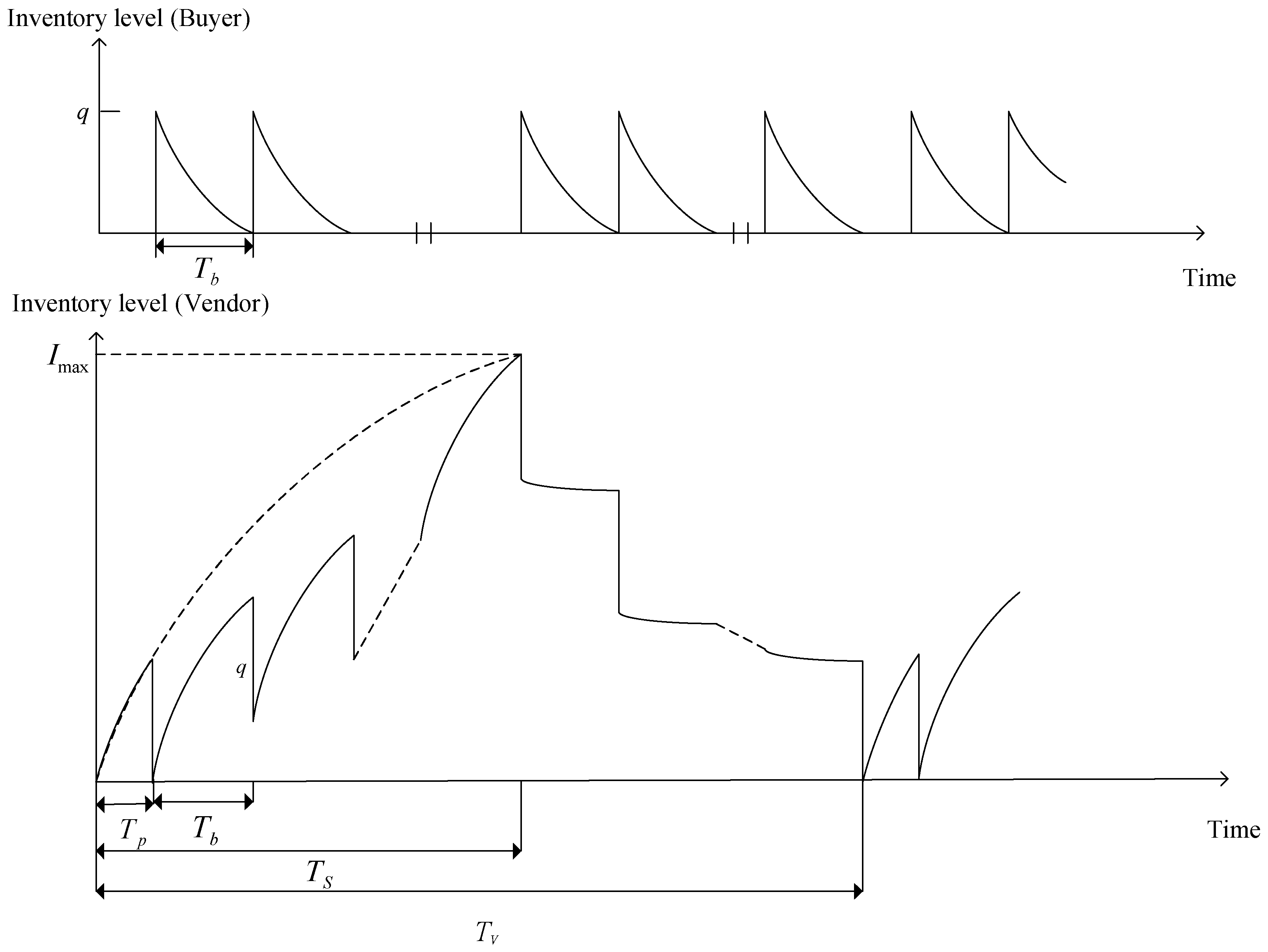
In this paper, we investigate an integrated production inventory model for deteriorating items under carbon tax policy and collaborative preservation technology investment. Firstly, we make a simple description about the production inventory system as follows: During a whole production cycle (the length of the period is $T_v$) in the supply chain, the buyer orders $Q$ units and requires the vendor to divide n consignments. The number of deliveries is equally $q$ units each shipment. The vendor begins shipping during the production period and ships to the buyer when the production quantity reaches q units in the first time period (the length of period is $T_p$). After that, the vendor ships q units at regular time intervals (the length of period is $T_b$). Because the vendor’s production rate is greater than the demand rate, it will stop producing and continue to ship regularly until all quantity is shipped when the production quantity reaches $I_{\max }$ (the length of period is $T_s$). The vendor and buyer’s inventory systems in a whole production cycle are shown as in Figure 1. Based on notation and assumptions mentioned above, we first established the total profits and amounts of carbon emissions per unit time for the buyer and vendor as follows.

3.1. Buyer’s Total Profit and Amount of Carbon Emissions

The buyer’s inventory level at time t during the replenishment cycle changes due to the market demand and the deterioration of the item (Figure 1) and is governed by the following differential equation:

$$\frac{dI(t)}{dt}+[1-m(\xi )]\theta I(t)=-D, 0\le t\le T_b.$$

(1)

By solving the differential equation in (1) with the boundary condition $I(T_b)=0$, the buyer’s inventory level is

$$I(t)=\frac{D}{1-m(\xi )\theta }\left[e^{[1-m(\xi )\theta (T_b-t)}-1\right],0\le t\le T_b.$$

(2)

From (2), the buyer’s order quantity per replenishment cycle $q=I(0)$ can be obtained, which implies

$$T_b=\frac{1}{[1-m(\xi )]\theta }\ln \left[\frac{[1-m(\xi )]\theta q+D}{D}\right].$$

(3)

The buyer’s total profit per replenishment cycle includes sale revenue, ordering cost, transportation cost, purchase cost, holding cost, and preservation technology investment. These components are evaluated as follows:

(a)

The buyer’s sale revenue per replenishment cycle is

$$pD{T}_b=\frac{pD}{[1-m(\xi )]\theta }\ln \left[\frac{[1-m(\xi )]\theta q+D}{D}\right].$$

(4)

(b)

The buyer’s ordering cost per replenishment cycle is A.

(c)

The buyer’s purchase cost is $vq$.

(d)

The buyer’s transportation cost including fixed and variable costs per replenishment cycle is given by $C_T+C_{t}q$.

(e)

The buyer’s holding cost is

$$h_b{\displaystyle {\int }_0^{T_b}I(t)dt}=h_b{\displaystyle {\int }_0^{T_b}\frac{D}{[1-m(\xi )]\theta }}[e^{[1-m(\xi )]\theta (T_b-t)}-1]dt$$

$$\hspace{1em}\hspace{1em}\hspace{1em}\hspace{1em}\hspace{1em}\hspace{1em}\hspace{1em}\hspace{1em} =\frac{h_b}{[1-m(\xi )]\theta }\left\{q-\frac{D}{[1-m(\xi )]\theta }\ln \left[\frac{[1-m(\xi )]\theta q+D}{D}\right]\right\}.$$

(5)

(f)

There is an investment in preservation technology for reducing the deterioration rate in order to preserve the products, which is $\xi$. Because the preservation technology investment is shared between the buyer and vendor, where the proportion of the buyer’s investment is a $\alpha$ ($0\le \alpha <1$), the preservation technology investment in reducing the deterioration rate per replenishment cycle for the buyer is $\alpha \xi /n$.

Because a production cycle consists of n replenishment cycles, the buyer’s total profit per production cycle (denoted by $T{P}_b(q,\xi )$) is

$$T{P}_b(q,\xi )=\frac{n\{[1-m(\xi )]\theta p+h_b\}D}{{[1-m(\xi )]}^2{\theta }^2}\ln \left[\frac{[1-m(\xi )]\theta q+D}{D}\right]-n(A+C_T)$$

$$-\left\{v+C_t+\frac{h_b}{[1-m(\xi )]\theta }\right\}nq-\alpha \xi .$$

(6)

Then, the amount of carbon emissions per production cycle for the buyer (denoted by $E_b(q,\xi )$) can be, respectively, calculated as follows:

$$E_b(q,\xi )=n(\widehat{A}+{\widehat{C}}_T)+\left\{{\widehat{C}}_t+\widehat{v}+\frac{{\widehat{h}}_b}{[1-m(\xi )\theta ]}\right\}nq-\frac{n{\widehat{h}}_{b}D}{{[1-m(\xi )]}^2{\theta }^2}\ln \left[\frac{[1-m(\xi )]\theta q+D}{D}\right].$$

(7)

3.2. Vendor’s Total Profit and Amount of Carbon Emissions

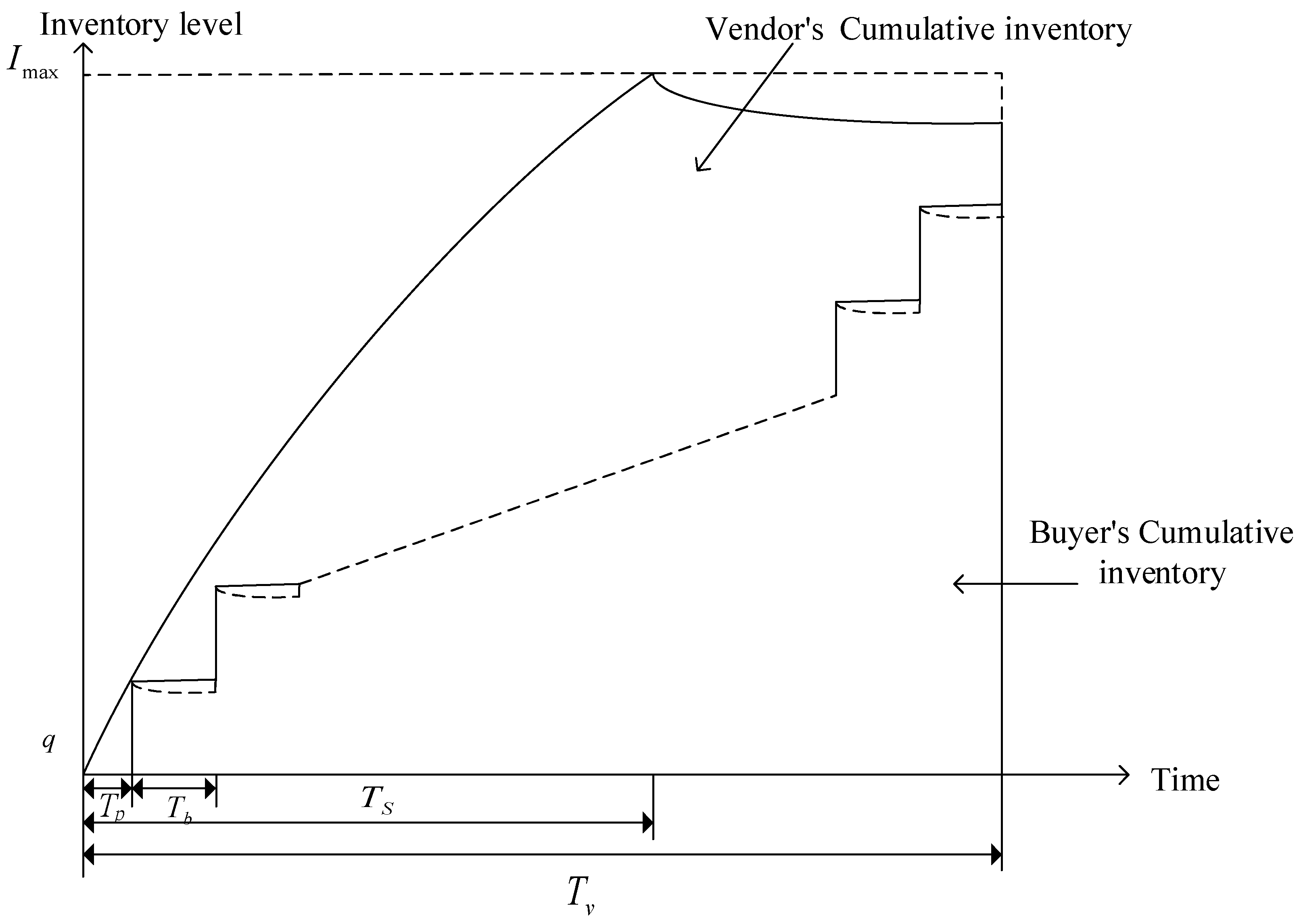
The vendor and buyer’s cumulative inventory can be shown as in Figure 2. During the time interval [0, $T_s$], the vendor’s inventory level changes, which results from production and the deterioration of the item. Hence, the vendor’s inventory level at time t during the time interval [0, $T_s$] is governed by the following differential equation:

$$\frac{d{I}_p(t)}{dt}+[1-m(\xi )]\theta I_p(t)=P, 0\le t\le T_s,$$

(8)

with boundary condition $I_p(0)=0$, and the solution of (8) is

$$I_p(t)=\frac{P}{[1-m(\xi )]\theta }[1-e^{-[1-m(\xi )]\theta t}], 0\le t\le T_s.$$

(9)

From Figure 2, it has $I_p(T_p)=q$, which implies

$$T_p=\frac{1}{[1-m(\xi )]\theta }\ln \left[\frac{P}{P-[1-m(\xi )]\theta q}\right].$$

(10)

During the time interval [$T_s$,$T_v$], the vendor’s inventory level just decreases because of the deterioration of the item, and its inventory level at time t during the time interval [$T_s$,$T_v$] is governed by the following differential equation:

$$\frac{d{I}_d(t)}{dt}+[1-m(\xi )]\theta I_d(t)=0, T_s\le t\le T_v.$$

(11)

Similarly, the vendor’s inventory level during the time interval [$T_s$,$T_v$] can be obtained with boundary condition $I_d(T_v)=nq$ by solving (11), which is given by

$$I_d(t)=nq{e}^{[1-m(\xi )]\theta (T_v-t)},T_s\le t\le T_v.$$

(12)

From (9) and (12), it is established that $I_p(T_s)=I_d(T_s)$, and it can be found that

$$T_s=\frac{1}{[1-m(\xi )]\theta }\ln \left[\frac{P+[1-m(\xi )]\theta nq{e}^{[1-m(\xi )]\theta T_v}}{P}\right].$$

(13)

Similarly, the supplier’s total profit per production cycle includes sale revenue, setup cost, production cost, holding cost, and preservation technology investment. These components are evaluated as follows:

(a)

The vendor’s sale revenue per production cycle is $vQ=vnq$.

(b)

The vendor’s setup cost per production cycle is $S$.

(c)

The vendor’s production cost per production cycle is

$$cP{T}_s=\frac{cP}{[1-m(\xi )]\theta }\ln \left[\frac{P+[1-m(\xi )]\theta nq{e}^{[1-m(\xi )]\theta T_v}}{P}\right].$$

(14)

(d)

Holding cost: From Figure 3, the vendor’s total inventory per production cycle is equal to the vendor’s cumulative inventory minus the buyer’s cumulative inventory and is given by ${\displaystyle {\int }_0^{T_S}{I}_p(t)dt+}{\displaystyle {\int }_{T_s}^{T_v}{I}_d(t)dt-}[q{T}_b(1+2+\dots +(n-1))]$. Hence the vendor’s total holding cost per production cycle is

$$\begin{array}{l}{h}_v\left\{\underset{}{\overset{}{{\displaystyle {\int }_0^{T_s}{I}_p(t)dt}+{\displaystyle {\int }_{T_s}^{T_v}{I}_d(t)dt}-[q{T}_b(1+2+\dots +(n-1))]}}\right\}\\ \hspace{1em}\hspace{1em}\hspace{1em}\hspace{1em}=h_v\left\{{\displaystyle {\int }_0^{T_s}\frac{P}{[1-m(\xi )]\theta }[1-e^{-[1-m(\xi )]\theta t}]dt}+{\displaystyle {\int }_{T_s}^{T_v}nq{e}^{e^{[1-m(\xi )]\theta (T_v-t)}}dt-\frac{n(n-1)q{T}_b}{2}}\right\}\end{array}$$

$$=h_v\left\{\frac{P{T}_s}{[1-m(\xi )]\theta }-\frac{nq}{[1-m(\xi )]\theta }-\frac{n(n-1)q{T}_b}{2}\right\}$$

$$\hspace{1em}\hspace{1em}\hspace{1em}\hspace{1em} =h_v\{\frac{P}{{[1-m(\xi )]}^2{\theta }^2}\ln \left[\frac{P+[1-m(\xi )]\theta nq{e}^{[1-m(\xi )]\theta T_v}}{P}\right]-\frac{nq}{[1-m(\xi )]\theta }$$

$$-\frac{n(n-1)q}{2[1-m(\xi )]\theta }\ln \left[\frac{[1-m(\xi )]\theta q+D}{D}\right]\}.$$

(15)

(e)

Similarly, the preservation technology investment is shared between the buyer and vendor, where the proportion of the vendor’s investment is a $1-\alpha$ ($0\le \alpha \le 1$), and the preservation technology investment in reducing the deterioration rate per production cycle for the vendor is $(1-\alpha )\xi$.

Consequently, the vendor’s total profit per production cycle (denoted by $T{P}_v(T_v,q,n,\xi )$) is

$$T{P}_v(T_v,q,n,\xi )=vnq-S-\frac{cP}{[1-m(\xi )]\theta }\ln \left[\frac{P+[1-m(\xi )]\theta nq{e}^{[1-m(\xi )]\theta T_v}}{P}\right]$$

$$-h_v\{\frac{P}{{[1-m(\xi )]}^2{\theta }^2}\ln \left[\frac{P+[1-m(\xi )]\theta nq{e}^{[1-m(\xi )]\theta T_v}}{P}\right]-\frac{nq}{[1-m(\xi )]\theta }$$

$$-\frac{n(n-1)q}{2[1-m(\xi )]\theta }\ln \left[\frac{[1-m(\xi )]\theta q+D}{D}\right]\}-(1-\alpha )\xi .$$

(16)

Then, the amount of carbon emissions per unit time for the vendor (denoted by $E_v(T_v,q,n,\xi )$) can be, respectively, calculated as follows:

$$E_v(T_v,q,n,\xi )=\widehat{S}+\frac{\widehat{c}P}{[1-m(\xi )]\theta }\ln \left[\frac{P+[1-m(\xi )]\theta nq{e}^{[1-m(\xi )]\theta T_v}}{P}\right]$$

$$\hspace{1em}\hspace{1em}\hspace{1em}\hspace{1em}\hspace{1em}\hspace{1em}\hspace{1em}\hspace{1em}\hspace{1em}+{\widehat{h}}_v\{\frac{P}{{[1-m(\xi )]}^2{\theta }^2}\ln \left[\frac{P+[1-m(\xi )]\theta nq{e}^{[1-m(\xi )]\theta T_v}}{P}\right]-\frac{nq}{[1-m(\xi )]\theta }$$

$$\hspace{1em}\hspace{1em}\hspace{1em}-\frac{n(n-1)q}{2[1-m(\xi )]\theta }\ln \left[\frac{[1-m(\xi )]\theta q+D}{D}\right]\}.$$

(17)

When the vendor and buyer have decided to share resources to undertake mutually beneficial cooperation, the joint total profit per unit time, which is a function of $T_v$, $q$, $n$, and $\xi$ (denoted by $JTP(T_v,q,n,\xi )$), can be obtained as the sum of the vendor’s and the buyer’s total profit per unit time divided by the length of cycle time ($T_b+T_v$) and is given by $JTP(T_v,q,n,\xi )=[T{P}_b(q,\xi )+T{P}_v(T_v,q,n,\xi )]/(T_b+T_v)$. When taking carbon tax into account, companies may be given incentives to account for the environmental costs through an externally applied carbon tax by the regulatory agencies. A simple tax schedule is a linear one; that is, companies pay an amount of C money units for each unit of carbon emitted (Arslan and Turkay [5]). Hence, the refined model with carbon tax (denoted by $\prod (T_v,q,n,\xi )$) is as follows.

$$\prod (T_v,q,n,\xi )=JTP(T_v,q,n,\xi )-\frac{C[E_b(q,\xi )+E_v(T_v,q,n,\xi )]}{T_b+T_v}$$

$$=\frac{1}{T_v+T_b}\{\frac{n\{[1-m(\xi )]\theta p+h_b+C{\widehat{h}}_b\}D}{{[1-m(\xi )]}^2{\theta }^2}\ln \left[\frac{[1-m(\xi )]\theta q+D}{D}\right]$$

$$-n(A+C\widehat{A}+C_T+C{\widehat{C}}_T)-(S+C\widehat{S})$$

$$-\left[C\widehat{v}+C_t+C{\widehat{C}}_t+\frac{(h_b+C{\widehat{h}}_b)-(h_v+C{\widehat{h}}_v)}{[1-m(\xi )]\theta }\right]nq$$

$$-\frac{\{[1-m(\xi )]\theta (c+C\widehat{c})+(h_v+C{\widehat{h}}_v)\}P}{{[1-m(\xi )]}^2{\theta }^2}\ln \left[\frac{P+[1-m(\xi )]\theta nq{e}^{[1-m(\xi )]\theta T_v}}{P}\right]$$

$$+\frac{(h_v+{\widehat{h}}_v)n(n-1)q}{2[1-m(\xi )]\theta }\ln \left[\frac{[1-m(\xi )]\theta q+D}{D}\right]-\xi \}.$$

(18)

By using the fact that $T_v=T_p+(n-1)T_b$ from Figure 2, the joint total profit per unit time can be reduced as $\prod (q,n,\xi )$. The purpose of this paper is to determine the optimal order quantity, the numbers of shipments, and preservation technology investment under the carbon tax regulation such that the joint profit function $\prod (q,n,\xi )$ has a maximum value. Because of the complexity of the model, and that $n$ is a integer, it is difficult to find the close forms of $q$, $n$, and $\xi$ and check the concavity of profit function directly. Alternatively, we verified the concavity by numerical analyses in the next section and develop a simple algorithm (Algorithm 1) to obtain solutions for buyers and vendors under the carbon tax regulation.

Algorithm 1 Procedure of finding the optimal solution

Step 1. Set n = 1.

Step 2. Find the values of $q_{(n)}$ and ${\xi }_{(n)}$ by setting $\partial \prod (q,n,\xi )/\partial q=0$ and $\partial \prod (q,n,\xi )/\partial \xi =0$.

Step 3. Substitute $q_{(n)}$ and ${\xi }_{(n)}$ into (18) to get $\prod (q_{(n)},{\xi }_{(n)},n)$

Step 4. Set $n=n+1$, and repeat Step 2 to get $\prod (q_{(n+1)},{\xi }_{(n+1)},n+1)$.

Step 5. If $\prod (q_{(n+1)},{\xi }_{(n+1)},n)<\prod (q_{(n)},{\xi }_{(n)},n)$, then $\prod (q^{*},{\xi }^{*},n^{*})=\prod (q_{(n)},{\xi }_{(n)},n)$. Hence, if $(q^{*},{\xi }^{*},n^{*})=(q_{(n)},{\xi }_{(n)},n)$ is the optimal solution, then stop. Otherwise, return to Step 4.

Once the optimal solution $(q^{*},{\xi }^{*},n^{*})$ is obtained, we can determine the buyer’s optimal order quantity $Q^{*}=n^{*}{q}^{*}$ and the optimal joint total profit $\prod (q^{*},{\xi }^{*},n^{*})$.

4. Numerical Analysis

In this section, we provide several numerical examples by referring to previous literature and use reasonable data to demonstrate the solution procedures. Further, we verify the concavity of the joint total profit function and conduct sensitivity analyses of the optimal solutions with respect to major parameters.

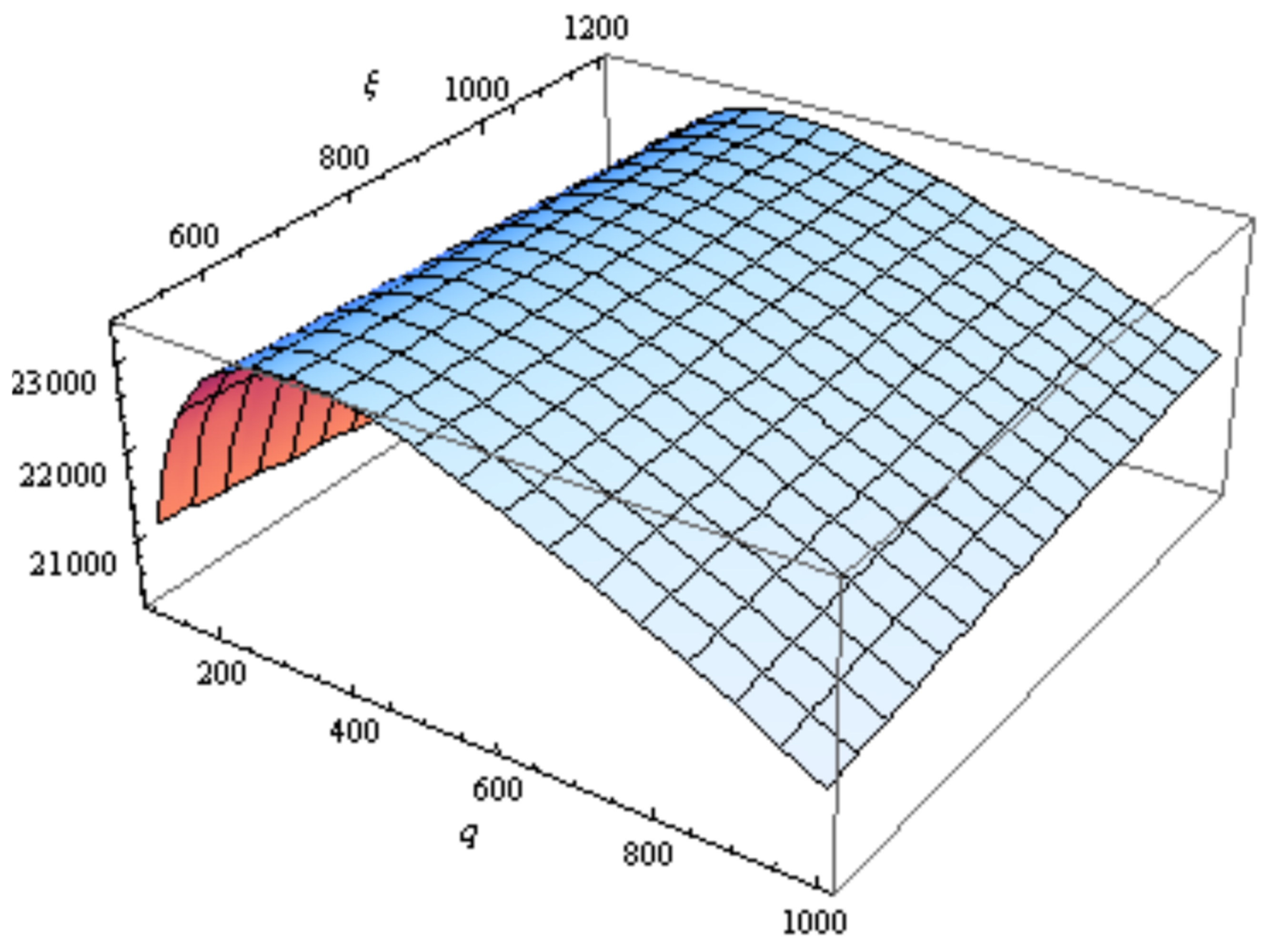
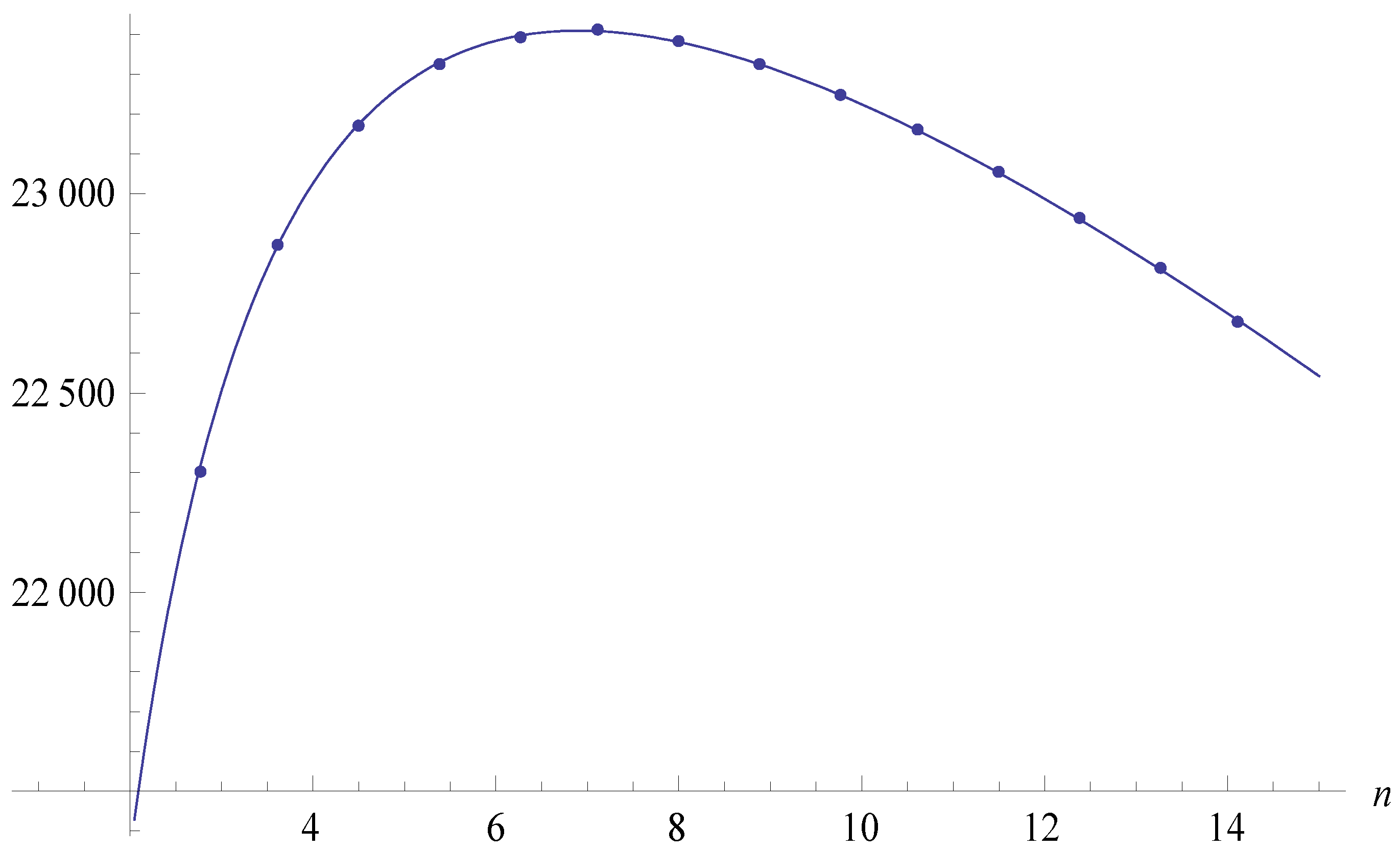
Example 1: Consider an inventory situation in which $D=1000$ units/year, $P=3000$ units/year, $A=\$200$/order, $\widehat{A}=50$ kg/order, $S=\$500$/setup, $\widehat{S}=200$ kg/setup, $c=\$5$/unit, $\widehat{c}=2$ kg/unit, $v=\$20$/unit, $\widehat{v}=2$ kg/unit, $p=\$40$/unit, $h_b=\$1$/unit/year, ${\widehat{h}}_b=0.5$ kg/unit/year, $h_v=\$0.3$/unit/year, ${\widehat{h}}_v=0.6$ kg/unit/year, $\theta =0.05$, $C_T=\$50$/ship, ${\widehat{C}}_T=3$ kg/ship, $C_t=\$3$/unit, $C=\$1$/unit, ${\widehat{C}}_t=1$ kg/unit, and $\alpha =0.5$. Moreover, we set the reduced deterioration rate function as $m(\xi )=1-e^{-0.001\xi }$. By applying the aforementioned algorithm, the vendor’s optimal number of shipments and shipping quantity were calculated as 7 and 345.999 units, respectively. The optimal order quantity of the buyer was 2421.993 units. The preservation technology investment was 748.726. The optimal joint total profit is as follows: $\prod (q^{*},{\xi }^{*},n^{*})=$ 23,409.4. Figure 3 displays the graphical illustration of the joint total profit function $\prod (q,\xi ,n)$ with respect to $q$ and $\xi$ for $n=7$, and Figure 4 illustrates the graphical illustration of the joint total profit function $\prod (q,\xi ,n)$ versus $n$ for $(q,\xi )=(345.999,748.726)$. That is, the concavity of the joint total profit function can be verified, and the obtained solutions are optimal for maximizing the joint total profit function.

Example 2: This example employs the same numerical analysis used in Example 1 and presents an analysis of different buyer and vendor investment-sharing ratios $\alpha \in \{0,0.1,0.2,0.3,\dots ,1\}$ for investment in technology for reducing the deterioration rate. We then obtained the optimal values for the vendor’s shipping quantity, investment in technology to reduce the deterioration rate, total profits of the buyer and vendor (respectively denoted by ${\prod }_b{}^{*}$ and ${\prod }_v{}^{*}$), and joint total profit per unit time (denoted by ${\prod }^{*}$). Moreover, we compared this case with the case without investment. The numerical analysis results are listed in

Table 1. Optimal solutions for various investment-sharing ratios.

$\mathit{\alpha }$	${\mathit{\xi }}^{*}$	${\mathit{q}}^{*}$	${\mathit{n}}^{*}$	${\prod }_{\mathit{b}}{}^{*}$	${\prod }_{\mathit{v}}{}^{*}$	${\prod }^{*}$
0	748.726	345.999	7	12,399.3	11,010.1	23,409.4
0.1	748.726	345.999	7	12,369.1	11,040.3	23,409.4
0.2	748.726	345.999	7	12,339.0	11,070.4	23,409.4
0.3	748.726	345.999	7	12,308.8	11,100.6	23,409.4
0.4	748.726	345.999	7	12,278.6	11,130.8	23,409.4
0.5	748.726	345.999	7	12,248.5	11,161.0	23,409.4
0.6	748.726	345.999	7	12,218.3	11,191.1	23,409.4
0.7	748.726	345.999	7	12,188.1	11,221.3	23,409.4
0.8	748.726	345.999	7	12,157.9	11,251.5	23,409.4
0.9	748.726	345.999	7	12,127.8	11,281.7	23,409.4
1	748.726	345.999	7	12,097.6	11,311.8	23,409.4
Without investment	0	293.723	6	12,142.3	11,248.6	23,391.0

. The results revealed that a change in α does not affect the decisions and the joint total profit of the integrated supply chain system. However, the larger the value of α, the more unfavorable the buyer’s profit, and the more favorable the seller’s profit. Moreover, compared with the case without investment, investing to reduce the deterioration rate is relatively beneficial in this with investment. From an individual viewpoint, if the buyer and vendor can jointly agree on the investment and decide the appropriate ratio (for example, α = 0.8 as in Table 1), the joint total profit of the supply chain system and the individual profit of each party increase. This result helps the supply chain members to develop a win–win strategy such that an integration of the sustainable supply chain system is achieved.

Example 3: In this example, sensitivity analysis demonstrates the effects of changes in the system parameters, such as on the optimal solution. The data used are the same as in Example 1, and the computational results are shown in

Table 2. Sensitivity analyses with respect to major parameters.

Parameters		${\mathit{\xi }}^{*}$	${\mathit{q}}^{*}$	${\mathit{n}}^{*}$	${\mathit{Q}}^{*}$	$\mathit{J}\mathit{T}{\mathit{P}}^{*}$
$D$	900	0	309.169	5	1545.845	20,986.3
	950	450.507	338.500	6	2031.000	22,194.6
	1000	748.728	345.999	7	2421.993	23,409.4
	1050	749.713	356.137	7	2492.959	24,628.5
	1100	956.198	354.373	8	2834.984	25,849.0
$P$	4000	973.429	343.205	8	2745.640	23,310.2
	4500	757.639	349.763	7	2448.341	23,359.2
	5000	748.728	345.999	7	2421.993	23,409.4
	5500	442.965	345.660	6	2073.960	23,459.1
	6000	0	325.073	5	1625.365	23,513.0
$A$	150	0	276.107	6	1656.642	23,562.0
	175	617.004	324.453	7	2271.171	23,482.2
	200	748.728	345.999	7	2421.993	23,409.4
	225	857.517	364.816	7	2553.712	23,340.8
	250	951.123	381.782	7	2672.474	23,275.5
$S$	400	327.090	328.075	6	1968.450	23,453.2
	450	713.918	340.176	7	2381.232	23,429.7
	500	748.728	345.999	7	2421.993	23,409.4
	550	781.712	351.604	7	2461.228	23,389.4
	600	813.089	357.017	7	2499.119	23,369.8
$c$	4	150.617	320.217	6	1921.302	24,434.8
	4.5	641.420	338.378	7	2368.646	23,920.7
	5	748.728	345.999	7	2421.993	23,409.4
	5.5	846.639	352.814	7	2469.698	22,900.1
	6	936.776	358.975	7	2512.825	22,392.5
$v$	18	748.728	345.999	7	2421.993	23,409.4
	19	748.728	345.999	7	2421.993	23,409.4
	20	748.728	345.999	7	2421.993	23,409.4
	21	748.728	345.999	7	2421.993	23,409.4
	22	748.728	345.999	7	2421.993	23,409.4
$h_b$	0.8	805.425	355.723	7	2490.061	23,443.5
	0.9	776.922	350.802	7	2455.614	23,426.3
	1	748.728	345.999	7	2421.993	23,409.4
	1.1	720.822	341.307	7	2389.149	23,392.7
	1.2	693.194	336.722	7	2357.054	23,376.3
$h_v$	0.2	884.660	371.214	7	2598.498	23,499.5
	0.25	815.814	358.215	7	2507.505	23,453.7
	0.3	748.728	345.999	7	2421.993	23,409.4
	0.35	371.582	334.808	6	2008.848	23,369.2
	0.4	290.253	321.217	6	1927.302	23,334.5
$C_T$	40	699.427	337.78	7	2364.460	23,438.0
	45	724.567	341.948	7	2393.636	23,423.6
	50	748.728	345.999	7	2421.993	23,409.4
	55	771.994	349.944	7	2449.608	23,395.4
	60	794.447	353.792	7	2476.544	23,381.5
$C_t$	2	732.606	344.864	7	2414.048	24,385.5
	2.5	740.694	345.434	7	2418.038	23,897.5
	3	748.728	345.999	7	2421.993	23,409.4
	3.5	756.705	346.559	7	2425.913	22,921.4
	4	764.630	347.115	7	2429.805	22,433.4
$p$	35	0	328.355	5	1641.775	18,577.8
	37.5	449.380	348.579	6	2091.474	20,986.5
	40	748.728	345.999	7	2421.993	23,409.4
	42.5	750.109	346.096	7	2422.672	25,839.6
	45	956.409	334.844	8	2678.752	28,274.3
$C$	0.8	987.168	351.159	8	2809.272	24,573.3
	0.9	759.768	353.350	7	2473.450	23,990.5
	1	748.728	345.999	7	2421.993	23,409.4
	1.1	452.581	343.743	6	2062.458	22,832.5
	1.2	456.151	339.378	6	2036.268	22,260.2
$\widehat{A}$	40	699.427	337.780	7	2364.460	23,438.0
	45	724.567	341.948	7	2393.636	23,423.6
	50	748.728	345.999	7	2421.993	23,409.4
	55	771.994	349.944	7	2449.608	23,395.4
	60	794.447	353.792	7	2476.544	23,381.5
$\widehat{S}$	160	721.038	341.360	7	2389.520	23,425.6
	180	735.035	343.698	7	2405.886	23,417.5
	200	748.728	345.999	7	2421.993	23,409.4
	220	762.126	348.266	7	2437.862	23,401.4
	240	775.251	350.500	7	2453.500	23,393.4
$\widehat{c}$	1.6	663.730	339.976	7	2379.832	23,818.3
	1.8	707.040	343.058	7	2401.406	23,613.7
	2	748.728	345.999	7	2421.993	23,409.4
	2.2	788.919	348.812	7	2441.684	23,205.5
	2.4	827.723	351.507	7	2460.549	23,001.8
$\widehat{v}$	1.6	742.305	345.547	7	2418.829	23,799.8
	1.8	745.520	345.774	7	2420.418	23,604.6
	2	748.728	345.999	7	2421.993	23,409.4
	2.2	751.924	346.224	7	2423.568	23,214.2
	2.4	755.112	346.447	7	2425.129	23,019.0
${\widehat{h}}_b$	0.4	776.922	350.802	7	2455.614	23,426.3
	0.45	762.789	348.387	7	2438.709	23,417.8
	0.5	748.728	345.999	7	2421.993	23,409.4
	0.55	734.738	343.640	7	2405.480	23,401.1
	0.6	720.822	341.307	7	2389.149	23,392.7
${\widehat{h}}_v$	0.48	1108.38	362.692	8	2901.536	23,518.8
	0.54	829.434	360.748	7	2525.236	23,462.7
	0.6	748.728	345.999	7	2421.993	23,409.4
	0.66	355.436	332.063	6	1992.378	23,362.2
	0.72	257.199	315.860	6	1895.160	23,321.0
${\widehat{C}}_T$	2.4	745.876	345.519	7	2418.633	23,411.1
	2.7	747.303	345.759	7	2420.313	23,410.3
	3	748.728	345.999	7	2421.993	23,409.4
	3.3	750.147	346.239	7	2423.673	23,408.6
	3.6	751.564	346.478	7	2425.346	23,407.7
${\widehat{C}}_t$	0.8	745.520	345.774	7	2420.418	23,604.6
	0.9	747.124	345.886	7	2421.202	23,507.0
	1	748.728	345.999	7	2421.993	23,409.4
	1.1	750.326	346.111	7	2422.777	23,311.8
	1.2	751.924	346.224	7	2423.568	23,214.2

. From the results shown in Table 2, the following observations can be made:

(1)

When the market demand is low (for example $D=900$) or the production rate is high (for example $P=6000$), the optimal preservation technology investment ${\xi }^{*}=0$, which implies that it is beneficial for the supply chain without preservation of technology investment. Further, as the market demand increases or the production rate decreases, the optimal vendor’s shipping quantity $q^{*}$, the buyer’s optimal order quantity $Q^{*}=n^{*}{q}^{*}$, and the optimal preservation technology investment ${\xi }^{*}$ increase. Finally, both demand and production rates have positive impacts on the joint total profit.

(2)

As the buyer’s ordering cost/the amount of carbon emissions per order, fixed shipping cost/the amount of fixed carbon emissions per shipment, variable shipping cost/the amount of carbon emissions per unit, the amount of carbon emissions associated per unit purchased, the vendor’s setup cost/the amount of carbon emissions per setup, or production cost/the amount of carbon emissions per unit produced increases, the optimal preservation technology investment ${\xi }^{*}$, the optimal vendor’s shipping quantity $q^{*}$, and the buyer’s optimal order quantity $Q^{*}=n^{*}{q}^{*}$ increase, but the optimal joint total profit decreases.

(3)

The buyer’s holding cost, vendor’s holding cost, amount of carbon emissions per unit of the inventory held for the buyer and the vendor, and the tax rate per unit of carbon emission have negative impacts on all the optimal preservation technology investment ${\xi }^{*}$, the optimal vendor’s shipping quantity $q^{*}$, the buyer’s optimal order quantity $Q^{*}=n^{*}{q}^{*}$, and the optimal joint total all profit.

(4)

When the buyer’s unit selling price increases, the optimal vendor’s shipping quantity $q^{*}$ increases first and then decreases. Further, all optimal preservation technology investment ${\xi }^{*}$, the buyer’s optimal order quantity $Q^{*}=n^{*}{q}^{*}$, and the optimal joint total profit increase with an increase in the buyer’s unit selling price.

(5)

The vendor’s supply price has no impact on the optimal solutions.

The aforementioned results can provide guidance on how to adjust the optimal shipping, ordering, and investing strategies for the entire supply chain system when different parameters change.

5. Conclusions

This study investigates a production inventory model for deteriorating items under a carbon tax policy and collaborative preservation technology investment from the perspective of supply chain integration. Our main purpose is to determine the optimal production, delivery, ordering, and investment policies for the buyer and vendor that maximize the joint total profit per unit time in consideration of the carbon tax policy. Because of the complexity of the model, we verify the concavity through numerical analysis and then develop an algorithm to obtain the solutions for the buyer and the vendor under the carbon tax regulation. Furthermore, we present several numerical examples to demonstrate the solution procedures, and we conduct sensitivity analyses of the optimal solutions with respect to major parameters to identify the following managerial implications:

(1)

If the buyer and vendor can jointly agree on the investment and decide the appropriate ratio, the joint total profit of the supply chain system and the individual profit of each party increase.

(2)

Investing in preservation technology to reduce the deterioration rate is usually beneficial for the proposed supply chain system, except when the market demand or unit price is low and the production rate is high.

(3)

When the market demand increases or the production rate decreases, the vendor’s optimal shipping quantity, buyer’s optimal order quantity, and the amount of preservation technology investment increase. Moreover, both demand and production rates have a positive influence on the joint total profit.

(4)

The higher the buyer’s ordering cost, buyer’s shipping costs, vendor’s setup cost, vendor’s production cost, or amount of carbon emissions due to ordering, shipping, purchasing, and producing, the higher the preservation technology investment, vendor’s optimal shipping quantity, and buyer’s optimal order quantity. However, all of these factors negatively influence the joint total profit of the system.

(5)

When the buyer’s or the vendor’s inventory-related costs and carbon emissions increase, the buyer’s order quantity and the vendor’s shipping quantity decrease. This decrease reduces the amount of investment and the joint total profit.

(6)

When the buyer’s unit selling price increases, the vendor’s optimal shipping quantity increases initially and then decreases. Furthermore, the optimal preservation technology investments, the buyer’s optimal order quantity, and the optimal joint total profit increase with an increase in the buyer’s unit selling price.

(7)

The vendor’s supply price has no influence on the optimal solutions. This is because the buyer and vendor are considered to be part of the same integrated supply system in which the buyer’s purchase cost or the seller’s sales revenue is ignored while calculating the joint total cost.

The proposed model could be extended in several ways. For example, the proposed inventory model could assume the demand rate as a function of selling price, time, and stock. Furthermore, when exploring integration strategies in a supply chain, a fair and reasonable framework should be adopted to ensure that members can share remuneration on system integration with each other. However, because of the differences in the power or preferences among supply chain members, the results differ from those in an equal reward system integration model. In this situation, we can discuss the competition and cooperative perspectives by using game theory, which is a study of mathematical models of conflict and cooperation between intelligent, rational decision-makers and investigates the equilibrium problem between them. Finally, the model could be generalized to allow for shortages, quantity discounts, inflation, trade credit, and other circumstances.

References

- Bouchery, Y.; Ghaffari, A.; Jemai, Z.; Dallery, Y. Including sustainability criteria into inventory models. Eur. J. Oper. Res. 2012, 222, 229–240. [Google Scholar] [CrossRef] [Green Version]
- Chen, X.; Benjaafar, S.; Elomri, A. The carbon-constrained EOQ. Oper. Res. Lett. 2013, 41, 172–179. [Google Scholar] [CrossRef]
- Benjaafar, S.; Li, Y.; Daskin, M. Carbon footprint and the management of supply chain: Insights from simple models. IEEE Trans. Autom. Sci. Eng. 2013, 10, 99–116. [Google Scholar] [CrossRef]
- Turkay, M. Environmentally conscious supply chain management. In Process Systems Engineering; Papageorgiou, L., Georgiadis, M., Eds.; Supply Chain Optimization; WILEY-VCH: Weinheim, Germany, 2008; Volume 3, pp. 45–86. [Google Scholar]
- Arslan, M.C.; Turkay, M. EOQ Revisited with Sustainability Considerations. Found. Comput. Decis. Sci. 2013, 38, 223–249. [Google Scholar] [CrossRef] [Green Version]
- Hua, G.; Cheng, T.; Wang, S. Managing carbon footprints in inventory management. Int. J. Prod. Econ. 2011, 132, 178–185. [Google Scholar] [CrossRef]
- Hua, G.; Cheng, T.C.E.; Wang, S. Managing Carbon Footprints in Inventory Control. Available online: http://ssrn.com/ abstract=1628953 (accessed on 24 November 2009).
- Battini, D.; Persona, A.; Sgarbossa, F. A sustainable EOQ model: Theoretical formulation and applications. Int. J. Prod. Econ. 2014, 149, 145–153. [Google Scholar] [CrossRef]
- He, P.; Zhang, W.; Xu, X.; Bian, Y. Production lot-sizing and carbon emissions under cap-and-trade and carbon tax regulations carbon tax regulations. J. Clean. Prod. 2015, 103, 241–248. [Google Scholar] [CrossRef]
- Song, J.; Leng, M. Analysis of the Single-Period Problem under Carbon Emissions Policies. Eval. Decis. Models Mult. Criteria 2012, 176, 297–313. [Google Scholar]
- Zhang, B.; Xu, L. Multi-item production planning with carbon cap and trade mechanism. Int. J. Prod. Econ. 2013, 144, 118–127. [Google Scholar] [CrossRef]
- Haddadsisakht, A.; Ryan, S.M. Closed-loop supply chain network design with multiple transportation modes under stochastic demand and uncertain carbon tax. Int. J. Prod. Econ. 2018, 195, 118–131. [Google Scholar] [CrossRef] [Green Version]
- Alizadeh, M.; Ma, J.; Marufuzzaman, M.; Yu, F. Sustainable olefin supply chain network design under seasonal feedstock supplies and uncertain carbon tax rate. J. Clean. Prod. 2019, 222, 280–299. [Google Scholar] [CrossRef]
- Goyal, S.K. An integrated inventory model for a single supplier-single customer problem. Int. J. Prod. Res. 1976, 15, 107–111. [Google Scholar] [CrossRef]
- Banerjee, A. A joint economic-lot-size model for purchaser and vendor. Decis. Sci. 1986, 17, 292–311. [Google Scholar] [CrossRef]
- Goyal, S.K. A joint economic-lot-size model for purchaser and vendor: a comment. Decis. Sci. 1988, 19, 236–241. [Google Scholar] [CrossRef]
- Lu, L. A one-vendor multi-buyer integrated inventory model. Eur. J. Oper. Res. 1995, 81, 312–323. [Google Scholar] [CrossRef]
- Goyal, S. A one-vendor multi-buyer integrated inventory model: A comment. Eur. J. Oper. Res. 1995, 82, 209–210. [Google Scholar] [CrossRef]
- Hill, R.M. The single-vendor single-buyer integrated production-inventory model with a generalized policy. Eur. J. Oper. Res. 1997, 97, 493–499. [Google Scholar] [CrossRef]
- Goyal, S.K.; Nebebe, F. Determination of economic production–shipment policy for a single-vendor–single-buyer system. Eur. J. Oper. Res. 2000, 121, 175–178. [Google Scholar] [CrossRef]
- Kelle, P.; Al-Khateeb, F.; Miller, P.A. Partnership and negotiation support by joint optimal ordering/setup policies for JIT. Int. J. Prod. Econ. 2003, 81, 431–441. [Google Scholar] [CrossRef]
- Giri, B.; Roy, B. A vendor-buyer integrated production-inventory model with quantity discount and unequal sized shipments. Int. J. Oper. Res. 2013, 16, 1–13. [Google Scholar] [CrossRef]
- Hill, R.M. The optimal production and shipment policy for the single-vendor single-buyer integrated production-inventory problem. Int. J. Prod. Res. 1999, 37, 2463–2475. [Google Scholar] [CrossRef]
- Ho, C.H.; Ouyang, L.Y.; Su, C.H. Optimal pricing, shipment and payment policy for an integrated supplier–buyer inventory model with two-part trade credit. Eur. J. Oper. Res. 2008, 187, 496–510. [Google Scholar] [CrossRef]
- Lin, Y.J. An integrated vendor–buyer inventory model with backorder price discount and effective investment to reduce ordering cost. Comput. Ind. Eng. 2009, 56, 1597–1606. [Google Scholar] [CrossRef]
- Lin, Y.J.; Ho, C.H. Integrated inventory model with quantity discount and price-sensitive demand. TOP 2011, 19, 177–188. [Google Scholar] [CrossRef]
- Lou, K.R.; Wang, W.C. A comprehensive extension of an integrated inventory model with ordering cost reduction and permissible delay in payments. Appl. Math. Model. 2013, 37, 4709–4716. [Google Scholar] [CrossRef]
- Sana, S.S. A production—inventory model in an imperfect production process. Eur. J. Oper. Res. 2010, 200, 451–464. [Google Scholar] [CrossRef]
- Sana, S.S. A production-inventory model of imperfect quality products in a three-layer supply chain. Decis. Support Syst. 2011, 50, 539–547. [Google Scholar] [CrossRef]
- Sucky, E. Coordinated order and production policies in supply chains. OR Spectr. 2004, 26, 493–520. [Google Scholar] [CrossRef]
- Wu, O.Q.; Chen, H. Optimal Control and Equilibrium Behavior of Production-Inventory Systems. Manag. Sci. 2010, 56, 1362–1379. [Google Scholar] [CrossRef]
- Wu, K.S.; Ouyang, L.Y. An integrated single-vendor single-buyer inventory system with shortage derived algebraically. Prod. Plan. Control 2003, 14, 555–561. [Google Scholar] [CrossRef]
- Yang, P.C.; Wee, H.M. Economic ordering policy of deteriorated item for vendor and buyer: An integrated approach. Prod. Plan. Control 2000, 11, 474–480. [Google Scholar] [CrossRef]
- Yang, P.C.; Wee, H.M. An integrated multi-lot-size production inventory model for deteriorating item. Comput. Oper. Res. 2003, 30, 671–682. [Google Scholar] [CrossRef]
- Yao, M.J.; Chiou, C.C. On a replenishment coordination model in an integrated supply chain with one vendor and multiple buyers. Eur. J. Oper. Res. 2004, 159, 406–419. [Google Scholar] [CrossRef]
- Ferguson, M.E.; Lystad, E.D.; Alexopoulos, C. Single Stage Heuristic for Perishable Inventory Control in Two-Echelon Supply Chains; Working paper; Georgia Institute of Technology: Atlanta, GA, USA, 2006. [Google Scholar]
- The Profit Experts. The 2011 Retail Profit Protection Report; The Profit Experts: Texas, TX, USA, 2011; Available online: http://www.prlog.org/11378377-the-2011-retail-profit-protection-report.html (accessed on 16 March 2011).
- Hsu, P.; Wee, H.; Teng, H. Preservation technology investment for deteriorating inventory. Int. J. Prod. Econ. 2010, 124, 388–394. [Google Scholar] [CrossRef]
- Dye, C.Y.; Hsieh, T.P. An optimal replenishment policy for deteriorating items with effective investment in preservation technology. Eur. J. Oper. Res. 2012, 218, 106–112. [Google Scholar] [CrossRef]
- Dye, C.Y. The effect of preservation technology investment on a non-instantaneous deteriorating inventory model. Omega 2013, 41, 872–880. [Google Scholar] [CrossRef]
- Dye, C.Y.; Hsieh, T.P. A particle swarm optimization for solving lot-sizing problem with fluctuating demand and preservation technology cost under trade credit. J. Glob. Optim. 2013, 55, 655–679. [Google Scholar] [CrossRef]
- He, Y.; Huang, H. Optimizing inventory and pricing policy for seasonal deteriorating products with preservation technology investment. J. Ind. Eng. 2013, 2013, 793568. [Google Scholar] [CrossRef]
- Singh, S.R.; Sharm, S. A global optimizing policy for decaying items with ramp-type demand rate under two-level trade credit financing taking account of preservation technology. Adv. Decis. Sci. 2013, 2013, 126385. [Google Scholar] [CrossRef]
- Shah, N.H.; Shah, D.B.; Patel, D.G. Optimal preservation technology investment, retail price and ordering policies for deteriorating items under trended demand and two level trade credit financing. J. Math. Model. Algorithms Oper. Res. 2015, 14, 1–12. [Google Scholar] [CrossRef]
- Tsao, Y.C. Joint location, inventory, and preservation decisions for non-instantaneous deterioration items under delay in payments. Int. J. Syst. Sci. 2016, 47, 572–585. [Google Scholar] [CrossRef]
Figure 1.
The vendor’s and buyer’s inventory systems in an entire production cycle.
Figure 2.
The vendor’s and buyer’s cumulative inventory.
Figure 3.
Graphical illustration of with respect to and for = 7.
Figure 4.
Graphical illustration of versus for .