Research on the Distribution of Pollution-Intensive Industries and Their Spatial Effects in China

1
Faculty of Geographical Science, Beijing Normal University, Beijing 100875, China
2
College of Geography and Environment, Shandong Normal University, Jinan 250358, China
*
Author to whom correspondence should be addressed.
Sustainability 2019, 11(19), 5378; https://0-doi-org.brum.beds.ac.uk/10.3390/su11195378
Submission received: 16 August 2019
/
Revised: 25 September 2019
/
Accepted: 25 September 2019
/
Published: 28 September 2019
(This article belongs to the Section Economic and Business Aspects of Sustainability)
Abstract
:Investigation of the spatial transfer laws and dynamic mechanisms of pollution-intensive industries (PIIs) is becoming a popular field in regional sustainable development. Based on the statistical data of 30 provinces (cities and districts) in China from 2000 to 2017, this paper applied the Gini coefficient and a redistribution index as well as spatial econometric approaches to explore the spatial distribution characteristics and spatial effects of China’s PIIs. PIIs in China have experienced two transition stages: ‘from north to south’ and ‘from east to central and west’, and the spatial distribution imbalance of PIIs has been gradually improved. In terms of industries, all PIIs in the northeast region were removed; PIIs in the eastern region not only transferred outward but also have experienced an agglomeration effect. The central and western regions were the main areas where transferring PIIs were settling. The distribution of PIIs in China showed a strong spatial correlation and a relatively stable path dependence. Through use of the spatial Dubin model, it is concluded that command-and-control environmental regulation and transportation costs had a negative impact on the distribution of PIIs in this region and a positive impact on the surrounding regions; thus, the pollution haven hypothesis was supported. Resource factors, technological innovation levels, and industrial structure—whether direct or indirect—had an inhibitory effect on the distribution of PII. Capital factors not only promoted the development of PIIs in this region, but also promoted it in other regions. Agglomeration economics had a positive impact on the distribution of PIIs in this region, and a negative impact on the surrounding regions.
1. Introduction
Since the beginning of the 1970s, governments in both developed and developing countries have enacted or revised a large number of laws and regulations to control environmental pollution [1]. Due to the compliance costs of local regulations along with local factor availability and prices, profit-maximizing producers who need cost reduction are more likely to choose loose environmental regulation (ER) locations [2]. In the 1970s, Walter et al. proposed the pollution haven hypothesis in response to increasingly stringent ERs and the gradual decline in the output value and export of PIIs in developed countries. The pollution haven hypothesis points out that PIIs tend to be located in areas with low environmental standards, which are considered “pollution ports” [3].
Market-oriented economic reform has gradually turned China into one of the most attractive destinations for foreign direct investment (FDI) in the world [4]. China has become the recipient of a large number of pollution-intensive industries (PIIs) from developed countries, which have caused serious environmental pollution problems such as hazy weather, black and smelly water, and ecological damage [5,6]. To solve prominent ecological and environmental problems and promote the formation of a green development mode, the government has constantly improved the environmental governance system to include multiple actors and policy tools [7,8]. Formal ER consists of command-and-control environmental regulation (CMCER) and market-oriented environmental regulation (MBER). The implementation of relevant laws, regulations, and policies can rapidly improve the environmental pollution situation. At the same time, MBERs—such as pollution discharge taxes, user taxes, and product taxes—can guide and encourage enterprises to reduce pollution levels [8,9]. In addition, the public can participate in environmental management and supervision through environmental decision-making, environmental letters and visits, environmental litigation, and other legal channels, thus affecting the environmental behavior of enterprises [10,11,12].
China is in a transition stage and its decentralized governance structure leads to obvious regional differences in ER, affecting the distribution of PIIs in China [13,14]. The implementation of a series of national strategies, such as “Western China Development” and “the Rise of Central China”, not only narrowed the development gap between other regions and the eastern regions but also promoted the transformation of PIIs from the eastern region with strict ERs to the central and western regions with more relaxed energy and emission policies [15,16]. Since 2008, the transfer PIIs from developed to developing regions in China has attracted broad attention [8,14,17,18]; however, there are few studies on the impact of different ERs on the redistribution of PIIs [19].
Using the panel data of PIIs from 30 provinces (cities and districts) in China with the period of 2000 to 2017, this paper constructed the ‘redistribution index’ covering the change of PII output value and quantity, and made a comprehensive analysis of the transfer of PIIs in China from the regional and industrial perspectives, reflecting the role of regional distinction and industrial categories in the choice of PII redistribution [3]. Spatial econometric approaches were used to explore the spatial effects of China’s PIIs. We try to draw a deep exploration of the following questions: (1) From the perspective of multiple regions and industries, what are the characteristics of the PII redistribution in China? (2) Do different ERs have any influence on the distribution of PIIs? (3) Does the distribution of PIIs have spillover effects between regions? (4) Do the influencing factors in existing studies change after considering the spatial effect?
We organized the rest of this article as follows. After the introduction, Section 2 summarizes the relevant research. Section 3 is a description of empirical methods, including the agglomeration index, Gini coefficient, redistribution index, spatial panel data model and data sources. Section 4 reports on the spatiotemporal changes in PIIs in China and then analyzes their spatial dependence and spillover effects. Section 5 summarizes and discusses the research results and puts forward the possible improvement direction in the future.
2. Literature Review
Since the 1990s, the impact of ER on industrial distribution and corporate performance has attracted research attention [3,20,21]; however, there is a heated debate about whether the pollution haven hypothesis and the Porter hypothesis are valid. The pollution haven hypothesis assumes that companies will respond to environmental regulations imposed by governments in different regions. Under strict environmental supervision, enterprises need to meet environmental requirements by purchasing new production equipment or finding new waste treatment methods, which will increase the production cost of enterprises. To reduce compliance costs for companies, business decision makers tend to locate production facilities in areas with less environmental regulation [22]. Since the beginning of the 21st century, the number of empirical studies on pollution haven hypothesis has steadily increased. Researchers have verified the pollution haven hypothesis by measuring the relationship between ER and foreign trade, FDI, and the distribution of PIIs [4,8,14,23]. They point out that environmental regulatory differences and enterprise types are key factors in the pollution haven hypothesis [24,25]; however, some have found through studies in many countries—such as those in Europe [24,26,27], Japan [28], and the United States [29]—that ER will not have a systematic impact on outward FDI and the distribution of most factories [2], and the application of new technologies, strategic cooperation, and information asymmetry will lead to the failure of ER [30,31].
The Porter hypothesis emphasizes that the strengthening of ER can stimulate enterprises to increase R&D investment [32], thus enhancing the ability of enterprises to innovate [13,33]. Technological progress will further promote the improvement of industrial productivity and behavioral changes in enterprises towards green development, and ultimately enhance their competitiveness [32,34]. Some heavily polluting companies still cluster in areas with strict ERs [3]; however, some have pointed out that the impact of ER on the competitiveness of enterprises may be small, and political, economic, regulatory, infrastructure, and investment risk are important factors affecting the site of enterprises [35,36,37]. In addition, the heterogeneity of enterprises and the role of government intervention cannot be ignored [38].
In view of the inconsistency of the test results of the two hypotheses, some have pointed out that the cause may be in the differences in research methodology, geographical scale and other specifics [17,39]. The analysis of early researchers was mostly based on cross-sectional data and seldom used panel data [2]. Moreover, there are great differences in the description of ERs, industrial redistribution, FDI, and other indicators [17]. Some have pointed out that enterprises would adopt different strategies in the face of strict ERs, and some enterprises would close their factories rather than choose another site [5,6,39]. Similarly, researchers have tended to adopt a ‘black or white’ attitude in the verification process, which implies ignorance or negation of other hypotheses [3,6].
In addition, scholars have made in-depth discussions on the factors affecting the distribution of PIIs from the aspects of agglomeration economy, globalization, transportation cost, technological progress, and path dependence. Studies have shown that the regional agglomeration of enterprises can not only reduce the cost of enterprise cooperation, but also increase the spillover effect of knowledge, so as to improve the specialization and competitiveness of enterprises [40]. Similarly, some scholars have emphasized that the increase of global production, the reduction of transportation cost and the progress of technology will have an important impact on the spatial organization of industrial production [41,42]. Arthur emphasizes the close correlation between the new site and the original site in the process of industrial layout, and the increasing return effect strengthens the path dependence of industrial site selection [43,44].
In general, previous studies emphasized the impact of ER on the transfer of PIIs and paid less attention to different types of ER tools and other influencing factors. From the perspective of research methods, although both qualitative and quantitative studies have been applied, most descriptions of the redistribution of PIIs use single indicators such as the number of enterprises or industrial output value. The spatial correlation between regions is neglected in this discussion of factors affecting the distribution of PIIs, causing inconsistencies in the research results.
3. Methodology
3.1. Definition and Data Sources
Different scholars have put forward different methods for defining PIIs. Some define them according to the environmental management cost of the industry, while others use the pollution emissions per unit of output value. In 2007, the Chinese government issued the first national pollution source census program, which not only established national and local key pollution source files, but also effectively mastered the number and regional distribution of pollution sources. According to the results of the first national survey of pollution sources, 11 heavy-polluting industries produced more than 80 percent of the pollutants in all industries. To ensure the objectivity, sustainability, and comparability of this research, 11 heavy-polluting industries concerned in the first national pollution sources survey program issued by the government were selected as PIIs in this paper [45,46,47]. The 11 heavy-polluting industries are as follows: agricultural food processing (S13), food manufacturing (S14), the textile industry (S17), leather and fur feathers (fine hair) and related products (S19), paper and paper products (S22), oil processing/coking and nuclear fuel processing (S25), chemical raw materials and chemical products manufacturing (S26), nonmetallic mineral products and rolling processing (S30), ferrous metal smelting and rolling processing (S31), nonferrous metal smelting and rolling processing (S32), and power/heat production and supply (S44).
According to China’s administrative division standards, 30 provinces (cities and districts) are selected as provincial administrative units in this study to reflect the status of social and economic development of different areas in China. According to the classification of China’s National Bureau of Statistics, we divided the areas into four regions: the eastern region, including Beijing, Tianjin, Hebei, Shanghai, Jiangsu, Zhejiang, Fujian, Shandong, Guangdong, and Hainan; the central region, including Shanxi, Anhui, Jiangxi, Henan, Hubei, and Hunan; the western region, including Inner Mongolia, Guangxi, Chongqing, Sichuan, Guizhou, Yunnan, Shaanxi, Gansu, Qinghai, Ningxia, and Xinjiang; and the northeast region including Liaoning, Jilin, and Heilongjiang. Data of this study were obtained from different Chinese statistical yearbooks, including the China Environmental Statistical Yearbook, China Statistical Yearbook, China Industrial Economy Statistical Yearbook (name changed to China Industry Statistical Yearbook after 2013), China Labor Statistics Yearbook, Statistical Yearbook of China’s High-Tech Industry, China Statistical Yearbook on Science and Technology, Yearbook of China Transportation & Communication and statistical yearbooks of provinces and cities. The research covers the years from 2000 to 2017. Due to the lack of data, Tibet was not included in the study. Additionally, to ensure data consistency, values were corrected for inflation to a constant 2000 level.
3.2. Methods for Measuring Industrial Distribution
In this paper, the following indicators and methods are adopted to study the spatiotemporal changes of the distribution of PIIs in China. First of all, an overall distribution index () which is defined by every region’s proportion of PIIs output is introduced. The changes of can reflect the changing location of PIIs in China [17]. Formula is
where n is the number of regions, and refers to the gross output value of all PIIs in province (city or district) i during the period t.
Then, we use the Gini coefficient (Gi) to describe the dispersion and the trend of geographical concentration of PIIs in China. The Gini coefficient is between 0 and 1. A higher (lower) value reflects a more concentrated (dispersed) enterprises. The Gini coefficient is [48]
where N represents the number of regions, μ represents the average of the proportion of polluting sector i in each region, is the gross output value of polluting sector i in the whole research area, and , are the gross output value of polluting sector i in province (city or district) j and province (city or district) k. The following formula can be used to simplify the computation [49]
The last, the location quotient index (), is widely used by scholars to study the degree of industrial agglomeration in a certain area [3,8,50]. Researchers have used the change in to measure the extent of industrial relocation of PIIs across regions [8]; however, industrial transfer includes not only the rise and fall of industrial production share in different regions but the partial or overall migration of industry in a geographical location, manifested in the change of industrial quantity. On this basis, we construct a redistribution index () to study the spatial relocation of PIIs in China. The formula is
where represents the output value of industry i of region j, represents the national output value of industry i, represents the number of industries i of region j, and t represents the time period from to . Industry i is relocated to region j in period t if the index is greater than 0. Otherwise, a negative index shows that industry i has relocated away from region j in period t. The greater the absolute value of the index, the higher the degree of industrial redistribution.
3.3. Spatial Econometrics Analysis
According to Tobler’s first geographic law, all objects on earth are related to each other, and closer objects are more connected than farther ones [50]. When studying the layout of PIIs in China, the traditional panel data method without consideration of the spillover effect of neighboring provinces will produce certain deviations, so spatial econometrics analysis is adopted to study the layout and spatial effect of PIIs in various provinces. Spatial econometrics analysis mainly involves a test of spatial correlation and the selection of a spatial panel data model.
3.3.1. Global Moran index and Local Moran index
Spatial autocorrelation is an analytical method to test whether the observed value of a position in space is correlated with the value of its adjacent position. If the value of a position variable increases, the value of the variable in its surrounding position also increases, indicating that there is positive spatial autocorrelation between the two positions. On the contrary, it indicates that these two positions have negative spatial autocorrelation. The global Moran index examines the overall agglomeration, while the local Moran index reflects the agglomeration around a certain region. In this article, we introduce spatial sequence , where n = 30, is the observed value of each province. The global and local Moran indices are
where = is the sample variance, and is a binary adjacency symmetric spatial weight matrix of region i and region j. The initial measure of spatial autocorrelation is based on the idea of binary adjacency between spatial units [51]. The form of under this definition is [52]
where i ∈ [1, n], j ∈ [1, m]. n and m are the number of regions.
According to the judgment method of adjacency, the contiguity weights can be divided into Rook weights and Queen weights. The form of under the rule of Rook weights is [53]
i and j have the same meaning as Equation (9).
The form of under the rule of Queen weights is
i and j have the same meaning as Equation (9).
The Moran index ranges from −1 to 1. If the value of Moran index is higher than 0, it means positive autocorrelation, high value and high value cluster, low value and low value cluster among provinces. If the Moran index is less than 0, it is negatively correlated, and the high and low values are clustered together. The local Moran scatter diagram can reflect the spatial agglomeration of PIIs in various provinces.
3.3.2. Spatial Panel Data Model
Space panel model can be divided into space lag model (SAR), space error model (SEM) and spatial durbin model(SDM) [54,55]. When the explained variable of the spatial unit is affected by the explained variable of the adjacent unit, the lagged item of the explained variable needs to be added into the general panel data model. This model is SAR, and the formula is [56]
When the error term of the spatial unit is affected by the error term of the adjacent unit, the spatially related error term needs to be added to the general panel data model. The model is SEM, and the formula is
The SDM is a general model that integrates the characteristics of SAR and SEM. The formula is
In Equations (12)–(14), represents the explained variable and it is an n×1 order identity matrix. represents the explanatory variable. If the number of explanatory variables is m, is an n×m order identity matrix. represents the regression coefficient, and it is an m×1 order identity matrix. The represents the random error term. N is the number of spatial unit. W is an n×n spatial weight matrix. is the spatial autoregressive coefficient. is the coefficient of spatial correlation between regression residuals. is the random error vector. is the coefficient of exogenous interaction.
The selection of the space panel model is mainly based on the null hypothesis H0:θ = 0 and H0:θ + β = 0. If the two null hypotheses are rejected at the same time, the SDM is selected; otherwise, the SAR and the SEM should be selected. Specific choices can be distinguished by Wald test and LR test. If the values of Wald-spatial lag and Lr-spatial lag both pass the significance test, it indicates that SDM cannot be simplified to SAR or SEM. Otherwise, SDM can be simplified to SAR or SEM [52]. Elhorst referred the partial differential method to the spatial panel model and obtained the partial differential matrix by calculating the partial derivatives. The partial differential matrix is . The average value of the main diagonal elements of the matrix is the direct effect, while the average value of the non-main diagonal elements of the matrix is the indirect effect [57].
4. Findings and Interpretation
4.1. Distribution and Migration of PIIs
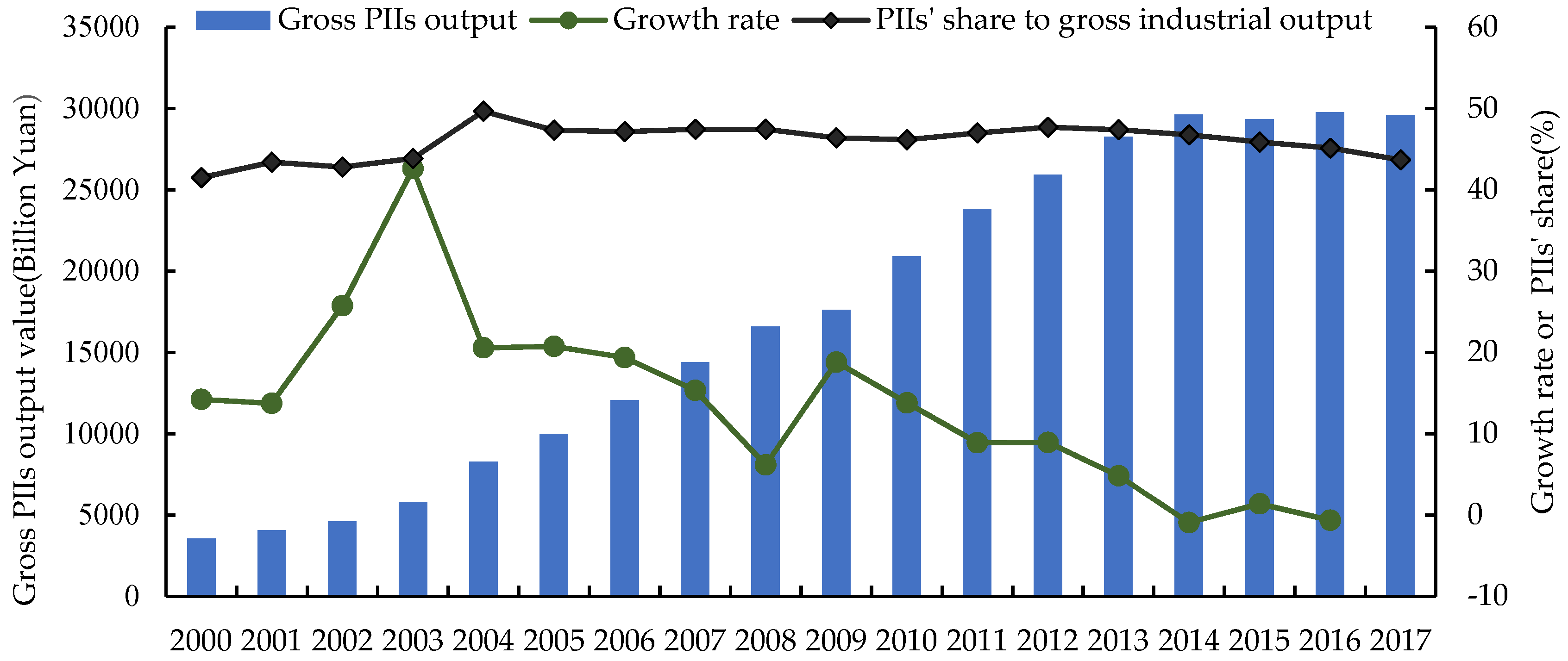
As indicated in Figure 1, there is an obvious increase in the sales value of Chinese PII output from 3553.84 billion yuan in 2000 to 29563.37 billion yuan in 2017 of which the growth rate turns to be 43.05% annually. At the same time, the ratio of PIIs to industrial output value first increased rapidly and then declined slowly. From 2000 to 2003 the increase in the PII growth rate benefited from the rapid development of industrial economy in Guangdong, Zhejiang, Jiangsu, Shandong, and other eastern coastal provinces. After 2003, with the transformation and upgrading of China’s economic structure, PIIs’ competitive advantage gradually weakened, resulting in a gradual decline in the proportion of PIIs.
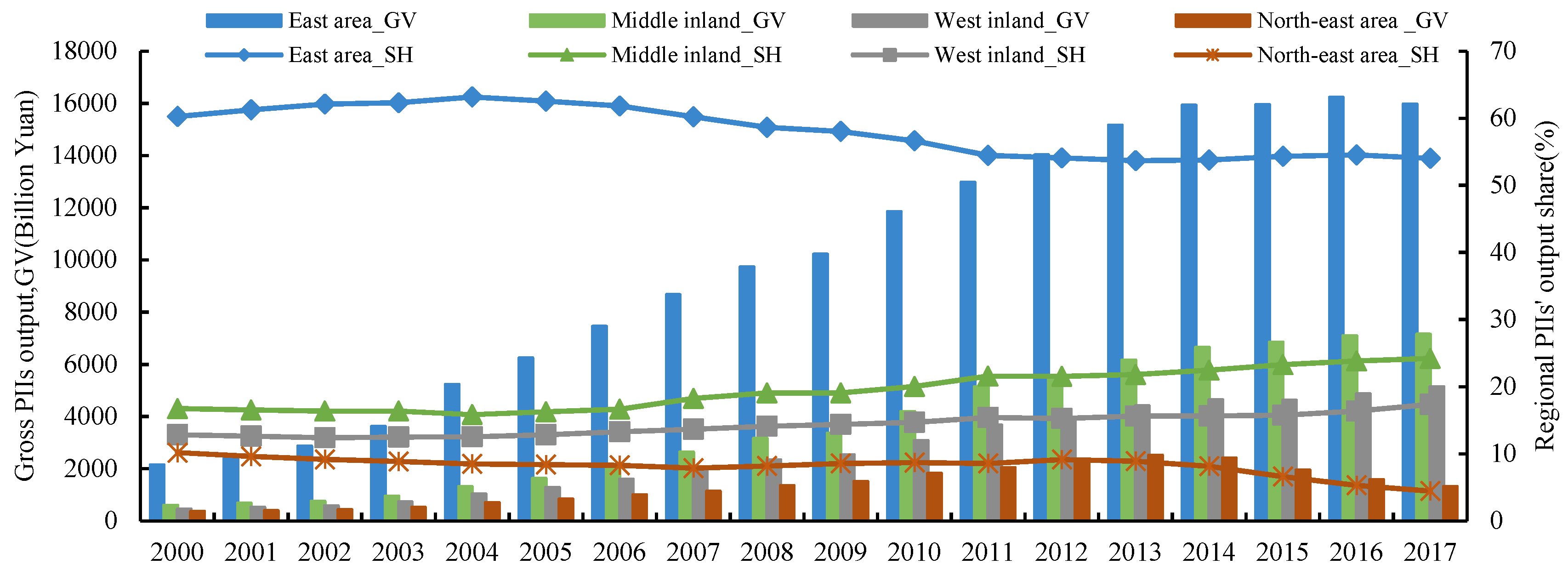
In terms of regions, China’s PIIs are gradually transferring from the eastern and northeastern regions to the central and western regions; the eastern and central regions have become the concentrated distribution areas for PIIs (Figure 2). The average annual growth rates of the output values (GV) of PIIs in the eastern and northeast regions were 37.97% and 15.47%. In the eastern and northeastern regions, a trend towards de-industrialization is evident, with the proportion of PIIs falling from 60.27% and 10.17% in 2000 to 54.01% and 4.44% in 2017. The average annual growth rate of the output value of PIIs in the central region and western regions was 64.90% and 60.26%. With the rapid development of industrial economy, the proportion of PIIs in the central and western regions increased from 16.73% and 12.84% in 2000 to 24.20% and 17.35% in 2017.
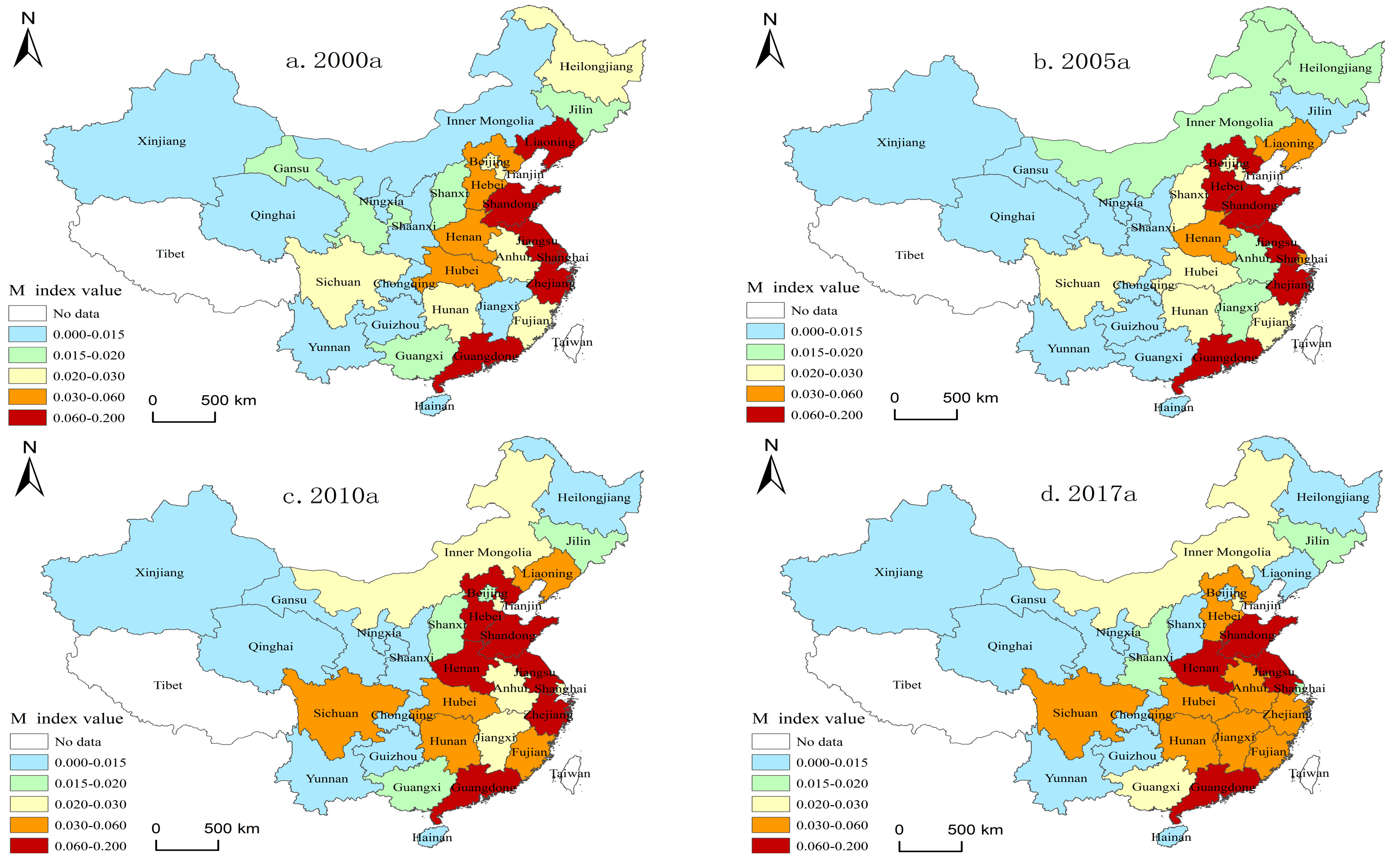
As shown in Figure 3, the M value distribution of provinces (cities and districts) in China in 2000, 2005, 2010 and 2017, confirming the redistribution process of PIIs in China. In 2000, areas with a high M value were concentrated in the eastern coastal areas, which were open to the outside world to receive a large amount of FDI and to promote the development of PIIs. In 2005, PIIs were transferred ‘from north to south’, and M values in Liaoning, Jilin, Heilongjiang decreased significantly; the agglomeration trend in the eastern region was further strengthened, and M values in Hebei, Shanxi, and Inner Mongolia were significantly increased. In 2010, PIIs shifted to the central and western regions, and the M value of Henan, Hubei, Hunan, Anhui, Jiangxi, Sichuan, and Inner Mongolia increased significantly. In 2017, the M value in the eastern region further decreased, forming a ‘transitional’ spatial pattern of east, central, west, and northeast. From 2000 to 2017, the spatial distribution of PIIs in China has gone through two stages: ‘from north to south’ and ‘from east to middle and west’, and the unbalanced spatial distribution of PIIs has been gradually improved. From 2000 to 2017, the M value significantly decreased in Beijing, Shanghai, Zhejiang, Liaoning, Heilongjiang, and Gansu. Among them, Shanghai, Zhejiang, and Liaoning saw the most obvious decrease in M value, while Henan and Jiangxi saw the most obvious increase.
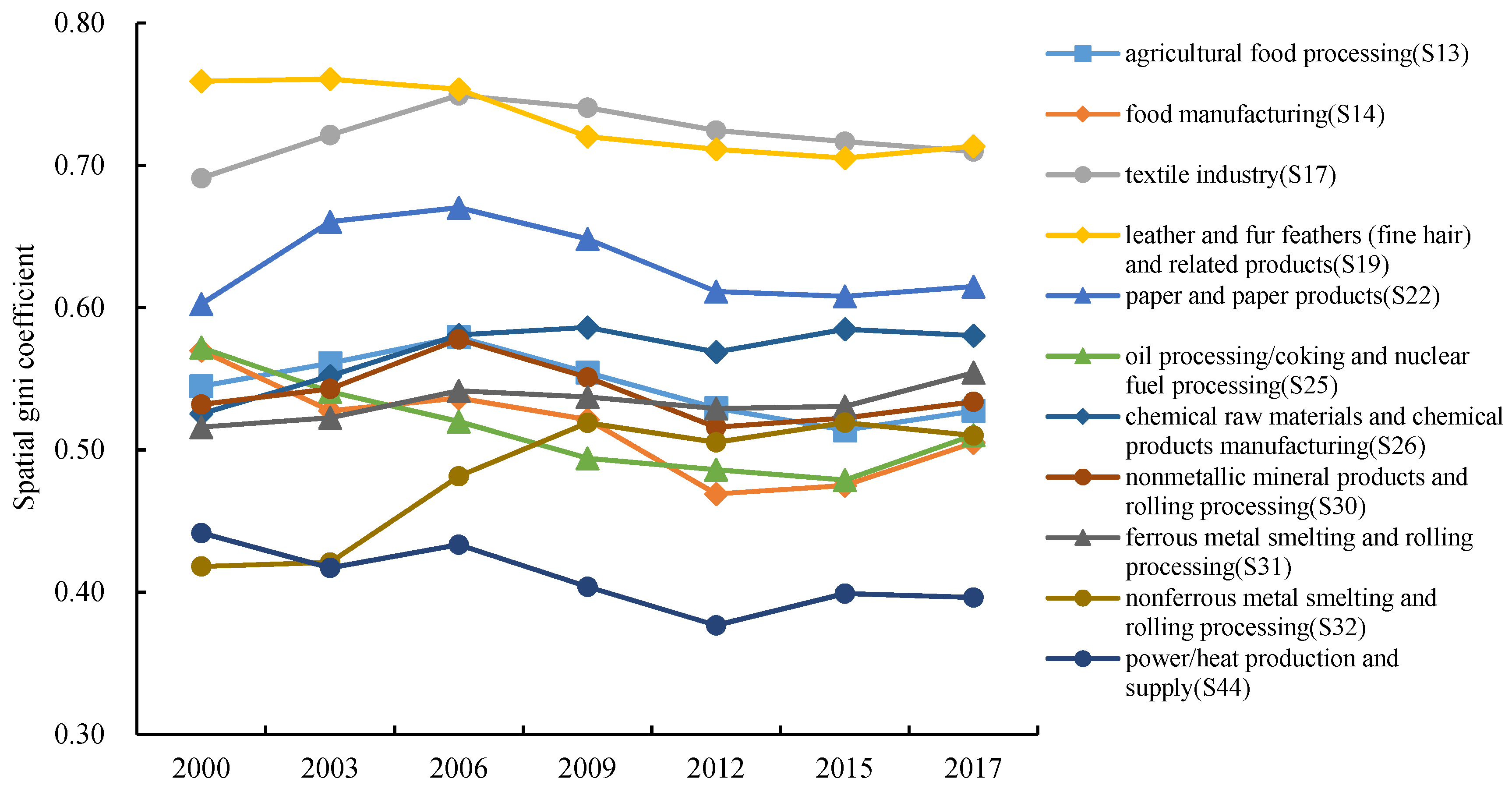
As shown in Figure 4, the spatial Gini coefficient of PIIs varies significantly among different industries. The textile industry (S17) and the leather and fur feathers (fine hair) and related products (S19) have spatial Gini coefficients higher than 0.70, which are much higher than other industries, and such industries are mostly concentrated in Fujian, Guangdong, Shandong, Jiangsu, and other provinces. The power/heat production and supply (S44) is more dispersed in space, with a Gini coefficient of 0.40 in 2017. The Gini coefficients of other industries are distributed between 0.40 and 0.70, with a moderate degree of spatial agglomeration and dispersion. According to the spatial Gini coefficient of PIIs, the redistribution of PIIs can be divided into three stages: 2000–2006 industrial decentralized development stage; 2006–2012 industrial transfer and diffusion stage; 2012–2017 industrial agglomeration development stage. From 2000 to 2006, the industries with reduced spatial Gini coefficient include food manufacturing (S14), leather and fur feathers (fine hair) and related products (S19), oil processing/coking and nuclear fuel processing (S25) and power/heat production and supply (S44), the spatial Gini coefficient of other PIIs increased. The period of the year 2006 to 2012, the spatial Gini coefficient of all PIIs have witnessed decreases of different extents except the nonferrous metal smelting and rolling processing (S32). Moreover, a slight rise could be found in all PIIs except the agricultural food processing (S13) and the textile industry (S17) from 2012 to 2017.
To identify the regional shift trend of each PII, Table 1 shows the index of each PII across China’s four major regions, eastern provinces (cities) and northeastern provinces from 2000 to 2017. The redistribution trend of PIIs is influenced by industry types and different regions. In addition to the textile (S17), paper and paper products (S22), oil processing/coking and nuclear fuel processing (S25), nonferrous metal smelting and rolling processing (S31) redistribution index is positive, the other PIIs’ redistribution index is negative in the eastern region. On the one hand, it indicates that the PIIs transfer out obviously; conversely it suggests that the eastern coastal areas—such as Shandong, Jiangsu, and Fujian—are more attractive for labor-intensive industries and resource-intensive industries. The central and western regions are the ones that try to recruit these PIIs from the east and northeast regions, but the industries they receive are different. Except for nonferrous metal smelting and rolling processing (S32) and power/heat production and supply (S44), other PIIs’ redistribution index in the central region are all positive, among which the larger ones are food manufacturing (S14), textile industry (S17), leather and fur feathers (fine hair) and related products (S19) and nonmetallic mineral products and rolling processing (S30). Except for nonferrous metal smelting and rolling processing (S32), other PIIs’ redistribution index in the western region are all positive, among which the larger are food manufacturing (S14), paper and paper products (S22), oil processing/coking, nuclear fuel processing (S25) and power/heat production and supply (S44); however, all PIIs redistribution index in northeast region are negative, indicating that all PIIs are transferring outward, and the PIIs with large redistribution index are food manufacturing (S14), ferrous metal smelting and rolling processing (S31), and nonferrous metal smelting and rolling processing (S32).
In general, from 2000 to 2017, all PIIs transfer out of northeast region. In the eastern region, PIIs not only transfer out but also have an agglomeration effect. The central and western regions are the main recipients of PIIs that transfer.
4.2. Spatial Correlation Analysis
Spatial correlation analysis is an important method for distinguishing traditional models from spatial econometric models. The traditional model ignores the spatial factor, resulting in a certain degree of error in the result. First, the spatial weight problem must be resolved for spatial correlation. In this article, we use Rook spatial weights to construct a spatial weight matrix. Since Hainan is not adjacent to any province, we assume that Hainan is adjacent to Guangdong by referring to most literature. According to the Moran index calculation formula, stata 14.0 software was used to calculate the global Moran’s I value of China from 2000 to 2017, as shown in Table 2. All Moran’s I values passed the test at a significance level of 10% over the years, and the average value was more than 0.2, indicating that there was a strong positive spatial correlation between the distribution of PIIs in various provinces. The distribution of PIIs is not random in space, and there is a certain agglomeration effect. In other words, provinces with more PIIs are adjacent, and provinces with fewer PIIs are adjacent.
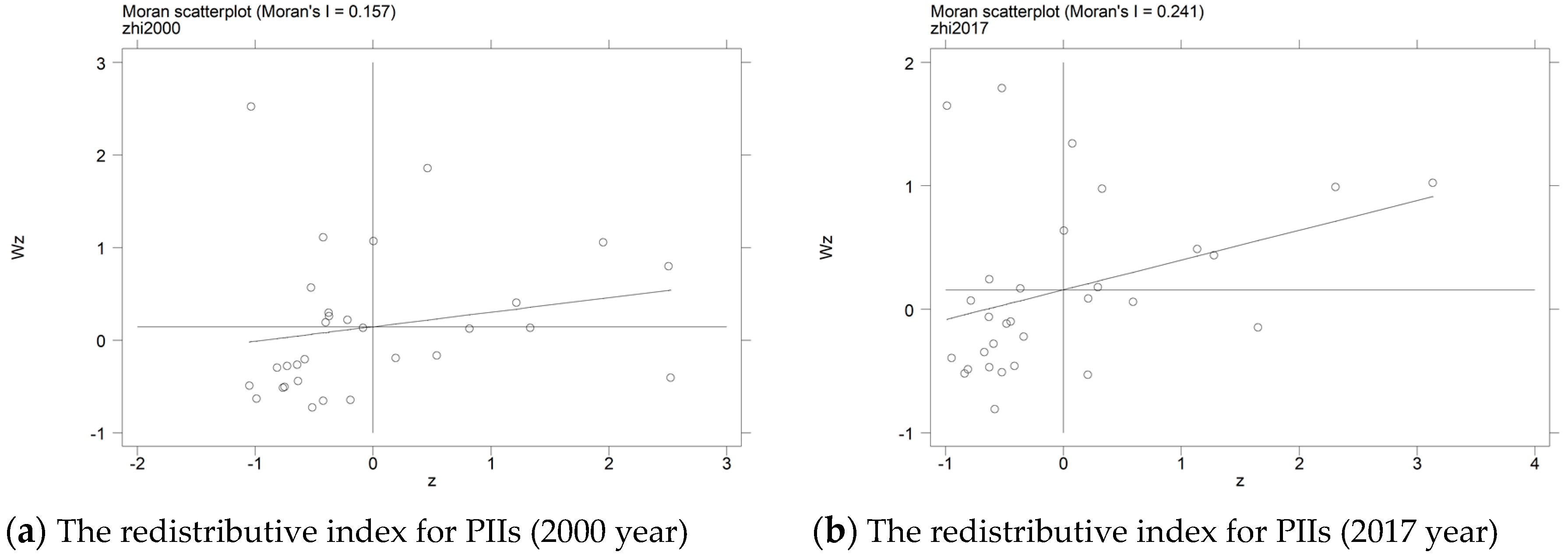
The local Moran scatter diagram reflects the correlation between regional observation values and their spatial lag, which can be divided into four quadrants. The first quadrant is high value-high value cluster (HH), the second quadrant is low value-high value cluster (LH), the third quadrant is low value-low value cluster (LL), and the fourth quadrant is high value-low value cluster (HL). The first and third quadrants indicate that the distribution of PIIs in these provinces are spatially positively autocorrelated, while the second and fourth quadrants are spatially negatively autocorrelated. Figure 5 shows the local Moran scatter diagram of provinces in 2000 and 2017. The distribution of PIIs in 2000 was mainly LL concentrated, and 12 provinces fell into the third quadrant, including Qinghai, Ningxia, Xinjiang, Guizhou, Yunnan, Sichuan, Gansu, Chongqing, Inner Mongolia, Shaanxi, Jilin, and Heilongjiang, which were mainly western and northeast provinces. Four provinces—including Shandong, Jiangsu, Zhejiang, and Shanghai—fell into the HH region which were eastern provinces. In 2017, the HH cluster and LL cluster of PIIs in all provinces increased significantly, and the number of the HH cluster provinces increased to seven—containing Handong, Jiangsu, Zhejiang, Fujian, Henan, Anhui, and Hunan—mainly eastern and central provinces. The number of LL cluster provinces increased to 14 (adding Beijing, Tianjin, and Liaoning and reducing Sichuan), and they were concentrated in the western and northeast regions. The distribution of PIIs shows a trend towards spatial agglomeration. Benefitting from its coastal geographical advantages, the eastern region attracts a large amount of FDI, and PIIs show high-value agglomeration; however, the development level of the western region is low, resulting in a low-value concentration of PIIs. By comparing the spatial agglomeration status in 2000 and 2017, containing that the number of high-agglomeration provinces and low-agglomeration provinces are increasing, and the distribution of PIIs has a strong path dependence. The high-value agglomeration area extends to the provinces of the central region, and the low-value agglomeration area extends to the provinces of the Bohai Bay area.
4.3. Spatial Panel Regression Analysis and Spillover Effect Decomposition
4.3.1. Spatial Panel Regression Analysis
In addition to being influenced by ERs, PIIs, as part of the manufacturing industry, have the same general rules as other manufacturing industries [58]. First, neoclassical trade theory emphasizes that factor endowment is an important factor guiding industrial location, so labor cost, technological innovation level, resource factors, and capital factors are added to the control variables to measure the impact of factor endowment on the distribution of PIIs [45,59]. Second, transportation costs, the agglomeration economy, globalization, and industrial structure have important influences on the distribution of PIIs [60].
To comprehensively investigate the factors affecting the spatial distribution of PIIs (SDPII), the variables are set as shown in Table 3: ① CMCER—The pollution haven hypothesis emphasizes that a region’s adoption of strong ERs will lead to the relocation of PIIs to surrounding areas. Therefore, strict environmental policy is gradually becoming an important factor affecting industrial spatial layout [14,18]. To calculate CMCER, the number of the newly implemented laws, regulations, and rules, and the number of environmental administrative penalty cases has been adopted by researchers [8,19]; there are random factors in implementing environmental policies due to the great freedom of local governments’ decision making, so these indicators may fail to reflect how environmental policies are implemented at the local level [19]. Considering the actual operation effect, data availability, and comparability of local government ERs, the government’s CMCER intensity is represented in this paper by the treatment input required for unit pollutant emissions. To some extent, this reflects the stringency of local CMCERs. The calculation formula is [61]
where is the investment amount of environmental pollution treatment in region i in year t, is the average investment amount of t year environmental pollution treatment in all regions of China, Pijt is the discharge amount of category j pollutants in region i in year t, and is the mean discharge amount of category j pollutants in various regions in t year. Pollutants include industrial waste gas, industrial wastewater, and industrial solid waste. The higher the CMCER value, the stricter the CMCER. the higher the intensity of the CMCER. ②MBER—Market incentive environmental regulation can not only change the economic cost or benefit of enterprises, but also affect the location choice and production decision of enterprises, so as to improve the environmental quality [18,34]. For the measurement of MBER, we reference existing studies of relevant scholars [8,62,63] and use the amount of pollutant discharge fees (in tens of thousands of yuan) divided by the industrial output value (in hundreds of millions of yuan) to express the intensity of MBER in each province (city and district). ③INER—Informal supervision introduces other relevant subjects to participate in environmental supervision. On the one hand, the public can make environmental appeals to government departments through letters, phone calls, and petitions, and supervise the government’s treatment of PIIs. On the other hand, the public can use media exposure to influence the market image of PIIs and force enterprises to make changes [8]. With respect to the measurement of INER, referring to Li and Ramanathan [19], the number of complaint letters concerning pollution and environmental issues are chosen to express the intensity of INER in each province (city and district). ④ Resource factors—The theory of comparative advantage points out that enterprises tend to locate in areas rich in raw materials in order to reduce production costs. Resource endowment selects the proportion of the number of mining employees to the total number of local employees to reflect the abundance of resources [64]. ⑤Capital factors—Neoclassical trade theory emphasizes that when the factor endowments of two countries are different, the product price of the region with abundant factor endowments is lower, which makes it easier to gain profits in international trade. This can also reflect the important role of capital in industrial distribution. Capital factor endowment is measured by the ratio of net fixed assets of an enterprise to GDP [45]. The net fixed assets of an enterprise is expressed as the original value of fixed assets minus the accumulated depreciation value. ⑥ Technological innovation level—The improvement of technical level can not only improve the production efficiency of enterprises, but also make up for the cost of pollution control of enterprises, thus affecting the site selection of enterprises. The level of technological innovation is expressed by the full-time equivalent of R&D personnel [64]. ⑦ Labor cost—In order to reduce production costs, enterprises tend to locate in regions with low wage levels, but some scholars believe that wage level is not the key factor for the transfer of PIIs. Labor factors use the average wage level of employees to measure regional labor cost differences [45]. ⑧ Transportation costs—The new economic geography points out that the relation between transportation cost and industrial location shows an inverted U shape. With the decrease of transportation cost, the spatial layout of industry tends to concentrate first and then disperse [8]. We use traffic density to represent the transportation costs. Traffic density is expressed by the ratio of the sum of railway operating mileage, highway mileage, and navigable mileage of inland waterways over the administrative area. ⑨Agglomeration economy—The centralized distribution of enterprises with strong industrial correlation degree can not only reduce production and transportation costs, but also facilitate information overflow and improve the degree of industrial specialization. Industrial agglomeration refers to the proportion of the total industrial output value of a region in the whole country [17,61]. ⑩ Globalization—Studies have pointed out that foreign direct investment is closely related to China’s industrial pollutant emissions, and the free flow of global trade and capital will lead to the transfer of PIIs to economically backward regions [4]. We use the degree of dependence on foreign trade to represent globalization. The degree of dependence on foreign trade is expressed by the ratio of the total value of imports and exports to GDP. ⑪ Industrial structure—The adjustment of industrial structure can not only optimize the allocation of resources, but also reduce the emission of regional pollutants, so as to promote the coordinated development of the region. Industrial structure adjustment is often accompanied by industrial transfer. Affected by changes in statistical data in approximately 2011, the adjustment of industrial structure is expressed by the ratio of the main business income of high-tech industry to the total industrial output value. Table 4 shows the descriptive statistics of each variable.
Before space panel regression, further evaluations of the space panel model can be made by comparing with the non-space panel model. Table 5 shows the regression results for the normal panel. As seen from the regression results, one of the two LM tests of space lag rejects the null hypothesis without space lag, and both LM tests of the space error test reject the null hypothesis without space error. The above tests further suggest that the influence of space factors cannot be ignored.
The existence of spatial effect makes the relationship between variables complicated, and the results of ordinary panel regression will have some deviation. After considering individual effect and time effect, we need to choose a fixed effect or random effect model. The Hausman test results (Table 6) reject the null hypothesis for the existence of random effects. Combined with the LR test results, the spatial panel model with fixed individuals is considered. Table 6 shows the regression results of three spatial panel models. Wald test rejects the null hypothesis of H0:θ = 0 and H0:θ + λβ = 0, indicating that SDM cannot be simplified into SAR and SEM.
(1) On the whole, INER, capital factors and agglomeration economy have positive effects on the distribution of the PIIs, and capital factors and agglomeration economy passed a 1% test of significance. CMCER, MBER, resource factors, technological innovation level, labor cost, transportation costs, globalization, and industrial structure have negative effects on the distribution of the PIIs. In addition, all other variables have passed the significance level test except that of MBER.
(2) From the analysis of specific indicators different ER tools have obvious differences on the distribution of PIIs. Strict CMCER can force enterprises to move, an important factor in promoting PII location changes. For 1% increase in strict CMCER intensity, the redistribution index for PIIs decreased by 0.074%. When the status of PIIs declines in the local industry, the local government will force enterprises to leave by adopting strict CMCERs in order to cost reduction for pollution control afforded by the local government. The pollutant discharge fees have a negative impact on the distribution of PIIs but fail the significance level test. The collection of sewage charges increases the cost of compliance, so many PIIs tend to locate in areas with low sewage charges to reduce their production costs. INER has a positive effect on the distribution of PIIs but fails the significance level test, possibly because the influence of INER on the distribution of PIIs is time-delayed [19].
(3) The influence of other factors on the distribution of PIIs is obviously different. Capital factors and agglomeration economy have positive effect on the distribution of PIIs. For 1% increase in capital factors and agglomeration economy, the redistribution index for PIIs increased by 0.111% and 0.714%. It shows that the increase of industrial investment can effectively promote the development of PIIs, and the agglomeration economy can not only improve the degree of enterprise specialization, but increase the industrial scale effect and knowledge spillover effect, thus improving the competitiveness of PIIs. Labor cost does a negative impact on PIIs’ distribution. For 1% increase in labor costs, the redistribution index for PIIs decreased by 0.175%. With the rise of labor prices, PIIs choose to transfer to less developed areas with lower labor costs to reduce production costs and improve the market competitiveness of products. Transportation costs have a negative effect on the distribution of the PIIs. For 1% increase in transportation costs, the redistribution index for PIIs decreased by 0.111%. This is mainly because the proposal of regional coordinated development strategy not only promotes the development of integrated transportation, but promotes the transfer of PIIs to other provinces. Resource factors, technological innovation level, globalization, and industrial structure have negative effects on the distribution of PIIs. With its rich resources and unique geographical advantages, the eastern coastal region has taken the lead in opening up to the outside world, not only enabling the eastern coastal region to attract a large volume of foreign investment, but also allowing the eastern coastal region to adopt a large amount of foreign advanced management experience and production technology. All these factors have promoted the rapid economic development of the region, but the development process has brought a series of ecological and environmental problems. With continuous improvement in people’s awareness of environmental protection, the optimization and upgrading of the industrial structure has forced the transfer of PIIs.
4.3.2. Decomposition of Spatial Spillover Effect
Based on the stata 14.0 software, the spatial direct effect and indirect effect of each variable are calculated (see in Table 7). From the perspective of the three ER tools, the direct and indirect effects of CMCER are -0.057 and 0.184, both of which have passed the significance level test. This indicates that CMCER can inhibit the distribution of PIIs in this region, but it promotes the distribution of PIIs in the surrounding provinces. That is, the intensification of CMCER in a region will promote the transfer of PIIs to surrounding areas. We get negative results of direct effects along with indirect effects of MBER, but failing in the significance level test, indicating that CMCER can promote the transfer of PIIs in local and surrounding areas, but the effect is not significant. The direct effect and indirect effect coefficients of INER are 0.013 and 0.047, and both have passed the significance level test. The direct and indirect effect coefficients of resource factors, technological innovation level, and industrial structure are all negative, and they all pass the significance level test, indicating that resource abundance, technological progress, and industrial structure adjustment not only promote the transfer of PIIs in this region but also promote the transfer of PIIs in surrounding provinces. It reflects that the low dependence of PIIs on resource factors and advanced technologies. The direct and indirect effects of capital factors are 0.134 and 0.247, indicating that the increase of industrial investment not only promotes the development of PIIs in this region but also promotes the development of PIIs in other provinces. The direct effect coefficients of labor cost, transportation costs and globalization are −0.160, −0.079, and −0.046, while the indirect effect coefficients are 0.155, 0.353, and 0.102. This indicates that labor costs, transportation costs, and globalization can inhibit the layout of PIIs in this region, but promote the layout of PIIs in surrounding areas; however, the indirect effects of labor costs and globalization fail the significance level test. Direct effects and indirect effects of the agglomeration economy coefficient are 0.678 and 0.408, and pass the significance level test. This suggests that the agglomeration economy can promote the specialization and cooperation of local enterprises and improve labor productivity to promote the development of local PIIs; however, the agglomeration economy inhibits the development of PIIs in surrounding areas.
5. Conclusions and Discussion
In recent years, the relationship between ERs and PIIs distribution in China has attracted extensive attention. This paper measured the movement of PIIs within China from 2000 to 2017 and analyzed the spatial effect of the distribution of PIIs. Unlike previous studies that focused on simple horizontal and vertical comparisons or traditional panel models, this paper introduced spatial factors and conducted a new empirical analysis of PIIs. We find that PIIs movement in China experienced two stages: ‘from north to south’ and ‘from east to central and west’. PIIs in the eastern region not only transferred outward, but show an agglomeration effect. The central and western regions were the main regions for PII development. All PIIs in the northeast region were transferred out. From the perspective of industry, China’s PIIs have gone through three stages: ‘decentralized development’, ‘transfer diffusion’, and ‘agglomeration development’. The distribution of PIIs in China showed a strong spatial correlation and a relatively stable path dependence. The distribution of PIIs is the result of the interaction between local and peripheral factors. Specifically, CMCER and transportation costs had a negative impact on the distribution of PIIs in this region, and a positive impact on the surrounding regions. Resource factors, technological innovation level, and industrial structure—whether direct or indirect—had an inhibitory effect on the distribution of PIIs. Capital factors not only promoted the development of PIIs in this region, but also promoted it in surrounding regions. Agglomeration economy had a positive impact on the distribution of PIIs in this region, and it had a negative impact on the surrounding regions.
In general, the geographical distribution pattern of China’s PIIs has undergone unambiguous adjustments under the combined action of various factors, leading to the redistribution of pollutants. Strict CMCER can effectively promote interregional transfer of PIIs, which has become an important measure for reduction of environmental pollution in many regions; however, MBER and INER do not have a significant impact on the distribution of PIIs, and their implementation effects need to be strengthened. In many regions, industrial structure decontamination is promoted by improving local ERs to reduce the emission of local pollutants, which does not effectively reduce the overall environmental pressure in China. Therefore, more research and development on production technology and pollution control technology is needed. At the same time, the central and western regions should be more rational in the treatment of industrial transfers from the eastern region. In view of the characteristics of PIIs, the characteristics of specific industries and the environmental carrying capacity of the region should be taken into account, and key industries to be contracted and industries to be restricted should be identified.
This paper verifies the establishment of the pollution haven hypothesis in China, that is, PIIs tend to locate in the central and western regions where ER is lax. However, we can also see that ER, as an exogenous force leading the location change of PIIs, does not necessarily lead to the transfer of PIIs. Agglomeration economy and path dependence are the key endogenous forces to promote enterprises to retain their original position. This also explains the shift of China’s PIIs to the east. Through research, we think that the transfer of PIIs is the result of the combined action of various internal and external forces dominated by ER and agglomeration economy. The change of the layout of PIIs depends not only on the intensity of ER and the role of agglomeration economy, but also on the type of industries and the surrounding conditions.
The distribution of PIIs is affected by various factors, and the distribution of enterprises of different sizes and types is affected by many factors. In addition, industries in different stages of development of demand will be greatly dissimilar. Due to data limitations, research on a fine geographical scale and on small-to-medium-sized polluters in this paper is obviously insufficient, suggesting subjects needing further improvement in future research.
Author Contributions
Methodology, M.R. and C.H.; Analysis and discussion: M.R., X.W., W.H., and W.Z.; Writing M.R., C.H., X.W., W.H., and W.Z.
Funding
This research received no external funding.
Conflicts of Interest
The authors declare no conflict of interest.
References
- Dasgupta, S.; Laplante, B.; Mamingi, N.; Wang, H. Inspections, pollution prices, and environmental performance: Evidence from China. Ecol. Econ. 2001, 36, 487–498. [Google Scholar] [CrossRef]
- Levinson, A. Environmental regulations and manufacturers’ location choices: Evidence from the census of manufactures. J. Public Econ. 1996, 62, 5–29. [Google Scholar] [CrossRef]
- Wu, J.W.; Wei, Y.D.; Chen, W.; Yuan, F. Environmental regulations and redistribution of polluting industries in transitional China: Understanding regional and industrial differences. J. Clean. Prod. 2019, 206, 142–155. [Google Scholar] [CrossRef]
- He, J. Pollution haven hypothesis and environmental impacts of foreign direct investment: The case of industrial emission of sulfur dioxide (SO2) in Chinese provinces. Ecol. Econ. 2006, 60, 228–245. [Google Scholar] [CrossRef]
- Liu, W.; Tong, J.; Yue, X. How Does Environmental Regulation Affect Industrial Transformation? A Study Based on the Methodology of Policy Simulation. Math. Probl. Eng. 2016, 2016, 1–10. [Google Scholar] [CrossRef]
- Zhu, S.; He, C.; Liu, Y. Going green or going away: Environmental regulation, economic geography and firms’ strategies in China’s pollution-intensive industries. Geoforum 2014, 55, 53–65. [Google Scholar] [CrossRef]
- Mol, A.P.J.; Carter, N.T. China’s environmental governance in transition. Environ. Polit 2006, 15, 149–170. [Google Scholar] [CrossRef]
- Zheng, D.; Shi, M. Multiple environmental policies and pollution haven hypothesis: Evidence from China’s polluting industries. J. Clean. Prod. 2017, 141, 295–304. [Google Scholar] [CrossRef]
- Zeng, D.Z.; Zhao, L. Pollution havens and industrial agglomeration. J. Environ. Econ. Manag. 2009, 58, 141–153. [Google Scholar] [CrossRef] [Green Version]
- Clark, M. Corporate environmental behavior research: Informing environmental policy. Struct. Chang. Econ. Dyn. 2005, 16, 422–431. [Google Scholar] [CrossRef]
- Wang, H.; Jin, Y. Industrial ownership and environmental performance: Evidence from China. Environ. Resour. Econ. 2007, 36, 255–273. [Google Scholar] [CrossRef]
- Zhang, B.; Bi, J.; Yuan, Z.W.; Ge, J.J.; Liu, B.B.; Bu, M.L. Why do firms engage in environmental management? An empirical study in China. J. Clean Prod. 2008, 16, 1036–1045. [Google Scholar] [CrossRef]
- Zhao, X.; Sun, B. The influence of Chinese environmental regulation on corporation innovation and competitiveness. J. Clean. Prod. 2016, 112, 1528–1536. [Google Scholar] [CrossRef]
- Wu, H.Y.; Guo, H.X.; Zhang, B.; Bu, M.L. Westward movement of new polluting firms in China: Pollution reduction mandates and location choice. J. Comp. Econ. 2017, 45, 119–138. [Google Scholar] [CrossRef]
- Li, H.M.; Wu, T.; Zhao, X.F.; Wang, X.; Qi, Y. Regional disparities and carbon “outsourcing”: The political economy of China’s energy policy. Energy 2014, 66, 950–958. [Google Scholar] [CrossRef]
- Zhu, J.; Rüth, M. Relocation or reallocation: Impacts of differentiated energy saving regulation on manufacturing industries in China. Ecol. Econ. 2015, 110, 119–133. [Google Scholar] [CrossRef]
- Shen, J.; Wei, Y.D.; Yang, Z. The impact of environmental regulations on the location of pollution-intensive industries in China. J. Clean. Prod. 2017, 148, 785–794. [Google Scholar] [CrossRef]
- Yang, J.; Guo, H.X.; Liu, B.B.; Shi, R.; Zhang, B.; Ye, W.L. Environmental regulation and the Pollution Haven Hypothesis: Do environmental regulation measures matter? J. Clean. Prod. 2018, 202, 993–1000. [Google Scholar] [CrossRef]
- Li, R.; Ramanathan, R. Exploring the relationships between different types of environmental regulations and environmental performance: Evidence from China. J. Clean Prod. 2018, 196, 1329–1340. [Google Scholar] [CrossRef]
- Birdsall, N.; Wheeler, D. Trade Policy and Industrial Pollution in Latin America: Where Are the Pollution Havens? J. Environ. Dev. 1993, 2, 137–149. [Google Scholar] [CrossRef]
- Brunnermeier, S.B.; Levinson, A. Examining the Evidence on Environmental Regulations and Industry Location. J. Environ. Dev. 2004, 13, 6–41. [Google Scholar] [CrossRef]
- Rezza, A.A. A meta-analysis of FDI and environmental regulations. Environ. Dev. Econ. 2014, 20, 185–208. [Google Scholar] [CrossRef]
- Bagayev, I.; Lochard, J. EU air pollution regulation: A breath of fresh air for Eastern European polluting industries? J. Environ. Econ. Manag. 2017, 83, 145–163. [Google Scholar] [CrossRef]
- Spatareanu, M. Searching for Pollution Havens: The Impact of Environmental Regulations on Foreign Direct Investment. J. Environ. Dev. 2007, 16, 161–182. [Google Scholar] [CrossRef]
- Dean, J.M.; Lovely, M.E.; Wang, H. Are foreign investors attracted to weak environmental regulations? Evaluating the evidence from China. J. Dev. Econ. 2009, 90, 1–13. [Google Scholar] [CrossRef] [Green Version]
- Leiter, A.M.; Parolini, A.; Winner, H. Environmental regulation and investment: Evidence from European industry data. Ecol. Econ. 2011, 70, 759–770. [Google Scholar] [CrossRef]
- Javorcik, B.S.; Wei, S.J. Pollution Havens and Foreign Direct Investment: Dirty Secret or Popular Myth? B E J. Econ. Anal. Policy 2004, 3, 1–34. [Google Scholar] [CrossRef]
- Kirkpatrick, C.; Shimamoto, K. The effect of environmental regulation on the locational choice of Japanese foreign direct investment. Appl. Econ. 2008, 40, 1399–1409. [Google Scholar] [CrossRef]
- Clark, D.P.; Marchese, S.; Zarrilli, S. Do Dirty Industries Conduct Offshore Assembly in Developing Countries? Int. Econ. J. 2000, 14, 75–86. [Google Scholar] [CrossRef]
- Regibeau, P.M.; Gallegos, A. Managed Trade, Trade Liberalisation and Local Pollution. B E J. Econ. Anal. Policy 2004, 4, 1–26. [Google Scholar] [CrossRef]
- Wu, X. Pollution Havens and the Regulation of Multinationals with Asymmetric Information. B E J. Econ. Anal. Policy 2004, 3, 1–25. [Google Scholar] [CrossRef]
- Yang, C.H.; Tseng, Y.H.; Chen, C.P. Environmental regulations, induced R&D, and productivity: Evidence from Taiwan’s manufacturing industries. Resour. Energy Econ. 2012, 34, 514–532. [Google Scholar]
- Porter, M.E.; Van Der Linde, C. Toward a New Conception of the Environment-Competitiveness Relationship. J. Econ. Perspect. 1995, 9, 97–118. [Google Scholar] [CrossRef]
- Zhao, X.L.; Zhao, Y.; Zeng, S.X.; Zhang, S.F. Corporate behavior and competitiveness: Impact of environmental regulation on Chinese firms. J. Clean Prod. 2015, 86, 311–322. [Google Scholar] [CrossRef]
- Jaffe, A.B.; Peterson, S.R.; Portney, P.R.; Stavins, R.N. Environmental regulation and the competitiveness of US manufacturing: What does the evidence tell us? J. Econ. Lit. 1995, 33, 132–163. [Google Scholar]
- Alpay, E.; Buccola, S.; Kerkvliet, J. Productivity growth and environmental regulation in Mexican and U.S. food manufacturing. Am. J. Agric. Econ. 2002, 84, 887–901. [Google Scholar] [CrossRef]
- Tole, L.; Koop, G. Do environmental regulations affect the location decisions of multinational gold mining firms? J. Econ. Geogr. 2011, 11, 151–177. [Google Scholar] [CrossRef]
- Zhou, Y.; Zhu, S.; He, C. How do environmental regulations affect industrial dynamics? Evidence from China’s pollution-intensive industries. Habitat Int. 2017, 60, 10–18. [Google Scholar] [CrossRef]
- Jeppesen, T.; Folmer, H. The confusing relationship between environmental policy and location behaviour of firms: A methodological review of selected case studies. Ann. Reg. Sci. 2001, 35, 523–546. [Google Scholar] [CrossRef]
- Malmberg, A.; Maskell, P. Towards an explanation of regional specialization and industry agglomeration. Eur. Plan. Stud. 1997, 5, 25–41. [Google Scholar] [CrossRef]
- Becattini, G.; Bellandi, M.; De Propris, L. A Handbook of Industrial Districts; Edward Elgar Publishing: Cheltenham, UK; Northampton, MA, USA, 2014; pp. 1–2. [Google Scholar]
- Bellandi, M.; Santini, E.; Vecciolini, C. Learning, unlearning and forgetting processes in industrial districts. Cambr. J. Econ. 2018, 42, 1671–1685. [Google Scholar] [CrossRef]
- Martin, R.; Sunley, P. Path dependence and regional economic evolution. J. Econ. Geogr. 2006, 6, 395–437. [Google Scholar] [CrossRef]
- Arthur, W.B. Increasing returns and path dependence in the economy. In Industry Location Patterns in the Importance of History; University of Michigan Press: Ann Arbor, MI, USA, 1994; pp. 49–67. [Google Scholar]
- Zhou, Y.; He, C.; Liu, Y. An empirical study on the geographical distribution of pollution-intensive industries in China. J. Nat. Res. 2015, 30, 1183–1196. [Google Scholar]
- Notice of The General Office of the State Council on Printing and Distributing the Plan for the First National Census of Pollution Sources. Available online: http://www.gov.cn/zwgk/2007-05/25/content_626141.htm (accessed on 25 May 2007).
- The First National Census of Pollution Sources. Available online: http://www.stats.gov.cn/tjsj/tjgb/qttjgb/qgqttjgb/201002/t20100211_30641.html (accessed on 11 February 2010).
- Qiu, F.D.; Jiang, T.; Zhang, C.M. Shan Y.B. Spatial relocation and mechanism of pollution-intensive industries in Jiangsu province. Sci. Geogr. Sin. 2013, 33, 789–796. [Google Scholar]
- He, C.; Wei, Y.D.; Xie, X. Globalization, institutional change, and industrial location: Economic transition and industrial concentration in China. Reg. Stud. 2008, 42, 923–945. [Google Scholar] [CrossRef]
- Tobler, W.R. A computer movie simulating urban growth in the detroit region. Econ. Geogr. 1970, 46, 234–240. [Google Scholar] [CrossRef]
- Moran, P.A.P. The Interpretation of Statistical Maps. J. R. Stat. Soc. Ser. B-Stat. Methodol. 1948, 10, 243–251. [Google Scholar] [CrossRef]
- Ye, C.; Sun, C.; Chen, L. New evidence for the impact of financial agglomeration on urbanization from a spatial econometrics analysis. J. Clean. Prod. 2018, 200, 65–73. [Google Scholar] [CrossRef]
- Hu, Y.; Zhang, J. Economic space evolution of Yangtze River Delta city group based on county scale. Econ. Geogr. 2010, 30, 1112–1117. [Google Scholar]
- Zhao, J.; Zhao, Z.; Zhang, H. The impact of growth, energy and financial development on environmental pollution in China: New evidence from a spatial econometric analysis. Energy Econ. 2019, 1–49. [Google Scholar] [CrossRef]
- Lesage, J.P.; Pace, R.K. Introduction to Spatial Econometrics; Chapman and Hall/CRC: New York City, NY, USA, 2009. [Google Scholar]
- Liu, H.C.; Fan, J.; Zeng, Y.X.; Guo, R. Spatio-temporal differences in carbon intensity in high-energy-intensive industry and its influence factors in China. Act. Ecol. Sin. 2019, 39, 1–13. [Google Scholar]
- Elhorst, J.P. Spatial Panel Data Models. In Spatial Econometrics; Springer: Berlin/Heidelberg, Germany, 2014; pp. 37–93. [Google Scholar]
- Shi, M.J.; Yang, J.; Long, W.; Wei, D.Y. Changes in geographical distribution of Chinese manufacturing sectors and its driving forces. Geogr. Res. 2013, 32, 1708–1720. [Google Scholar]
- Zheng, T.; Zhao, Y.; Li, J.; Tengfei, Z.; Yao, Z.; Jiarong, L. Rising labour cost, environmental regulation and manufacturing restructuring of Chinese cities. J. Clean. Prod. 2019, 214, 583–592. [Google Scholar] [CrossRef]
- Coughlin, C.C.; Segev, E. Location Determinants of New Foreign-Owned Manufacturing Plants. J. Reg. Sci. 2000, 40, 323–351. [Google Scholar] [CrossRef]
- Tian, G.H.; Miao, C.H.; Hu, Z.Q.; Miao, J.M. Environmental regulation, local protection and the spatial distribution of pollution-intensive industries in China. Act. Geogr. Sin. 2018, 73, 1954–1969. [Google Scholar]
- Guo, L.; Qu, Y.; Tseng, M. The interaction effects of environmental regulation and technological innovation on regional green growth performance. J. Clean. Prod. 2017, 162, 894–902. [Google Scholar] [CrossRef]
- Xie, R.; Yuan, Y.; Huang, J. Different types of environmental regulations and heterogeneous influence on “Green” productivity: Evidence from China. Ecol. Econ. 2017, 132, 104–112. [Google Scholar] [CrossRef]
- Xu, K.; Wang, J. An empirical study of a linkage between natural resource abundance and economic development. Econ. Res. J. 2006, 1, 78–89. [Google Scholar]
Figure 1.
Overall growth of PIIs in China, 2000–2017.

Figure 2.
Regional growth of PIIs in China, 2000–2017.

Figure 3.
The distribution pattern of sales output value of PIIs in China, 2000–2017.

Figure 4.
Spatial Gini coefficient of PIIs in China, 2000–2017.

Figure 5.
Local Moran scatter diagram of Chinese provinces, 2000–2017.


Table 1.
index of PIIs across China’s four major regions and key provinces, 2000–2017.
| Regions | S13 | S14 | S17 | S19 | S22 | S25 | S26 | S30 | S31 | S32 | S44 |
|---|---|---|---|---|---|---|---|---|---|---|---|
| Eastern region | −0.56 | −1.14 | 0.54 | −0.91 | 0.66 | 0.75 | −0.12 | −0.56 | 0.47 | −0.40 | −0.04 |
| Central region | 0.05 | 0.50 | 0.27 | 0.83 | 0.01 | 0.15 | 0.10 | 0.24 | 0.04 | −0.05 | −0.13 |
| Western region | 0.04 | 0.22 | 0.03 | 0.05 | 0.22 | 0.44 | 0.02 | 0.06 | 0.04 | −0.29 | 0.18 |
| Northeast region | 0.00 | −0.21 | −0.06 | −0.05 | −0.12 | −0.16 | −0.12 | −0.13 | −0.20 | −0.22 | −0.04 |
| Beijing | −0.04 | −0.17 | −0.03 | −0.02 | −0.04 | −0.07 | −0.05 | −0.05 | −0.05 | −0.03 | 0.06 |
| Tianjin | −0.04 | −0.05 | −0.05 | −0.04 | −0.02 | 0.06 | −0.11 | −0.02 | 0.02 | −0.04 | 0.00 |
| Hebei | −0.03 | −0.17 | 0.01 | 0.16 | −0.08 | 0.11 | −0.04 | −0.12 | 0.27 | −0.04 | −0.04 |
| Shanghai | −0.05 | −0.22 | −0.12 | −0.12 | −0.08 | −0.07 | −0.10 | −0.08 | −0.16 | −0.14 | −0.01 |
| Jiangsu | −0.11 | −0.15 | 0.13 | −0.05 | 0.13 | 0.02 | 0.02 | −0.09 | 0.19 | −0.14 | 0.08 |
| Zhejiang | −0.10 | −0.13 | 0.21 | −0.70 | 0.22 | 0.05 | 0.00 | −0.06 | 0.06 | −0.09 | 0.05 |
| Fujian | 0.00 | 0.04 | 0.15 | 0.11 | 0.15 | 0.02 | 0.01 | 0.01 | 0.02 | 0.00 | −0.04 |
| Shandong | −0.08 | 0.05 | 0.26 | −0.14 | 0.23 | 0.61 | 0.17 | 0.00 | 0.11 | 0.13 | 0.03 |
| Guangdong | −0.09 | −0.31 | −0.01 | −0.12 | 0.14 | −0.01 | −0.02 | −0.15 | 0.02 | −0.06 | −0.17 |
| Hainan | −0.01 | −0.04 | 0.00 | 0.00 | 0.01 | 0.02 | 0.00 | −0.01 | 0.00 | 0.00 | −0.01 |
| Liaoning | −0.11 | −0.15 | −0.05 | −0.07 | −0.07 | −0.07 | −0.09 | −0.12 | −0.16 | −0.18 | −0.04 |
| Jilin | 0.07 | 0.02 | 0.00 | 0.00 | 0.04 | −0.01 | −0.02 | 0.01 | −0.03 | −0.03 | 0.00 |
| Heilongjiang | 0.04 | −0.09 | −0.01 | 0.03 | −0.06 | −0.08 | −0.01 | −0.02 | −0.02 | −0.02 | 0.00 |
Note: agricultural food processing (S13), food manufacturing (S14), the textile industry (S17), leather and fur feathers (fine hair) and related products (S19), paper and paper products (S22), oil processing/coking and nuclear fuel processing (S25), chemical raw materials and chemical products manufacturing (S26), nonmetallic mineral products and rolling processing (S30), ferrous metal smelting and rolling processing (S31), nonferrous metal smelting and rolling processing (S32), power/heat production and supply (S44).
Table 2.
Moran index values of the distribution of PIIs in China’s provinces from 2000 to 2017.
| Year | Moran’s I | p-Value | Year | Moran’s I | p-Value |
|---|---|---|---|---|---|
| 2000 | 0.157 | 0.059 | 2009 | 0.204 | 0.022 |
| 2001 | 0.171 | 0.047 | 2010 | 0.202 | 0.025 |
| 2002 | 0.177 | 0.043 | 2011 | 0.208 | 0.021 |
| 2003 | 0.196 | 0.029 | 2012 | 0.229 | 0.013 |
| 2004 | 0.227 | 0.015 | 2013 | 0.223 | 0.015 |
| 2005 | 0.203 | 0.023 | 2014 | 0.239 | 0.011 |
| 2006 | 0.204 | 0.022 | 2015 | 0.251 | 0.008 |
| 2007 | 0.203 | 0.022 | 2016 | 0.251 | 0.008 |
| 2008 | 0.210 | 0.020 | 2017 | 0.241 | 0.010 |
Table 3.
Variables of the panel data model.
| Category | Definition (Unit) | Expected Sign |
|---|---|---|
| SDPII | The redistribution index (Rij) of PIIs | |
| CMCER | The treatment input required for unit pollutant emission (yuan) | − |
| MBER | Amount of pollutant discharge fees/industrial output value (%) | − |
| INER | Number of complaint letters concerning pollution and environmental issues (piece) | − |
| Resource factors | Number of mining employees/local employees (%) | + |
| Capital factors | Ratio of net fixed assets of an enterprise to GDP (%) | + |
| Technological level | Full-time equivalent of R&D personnel (man-year) | + |
| Labor cost | Average wage level of employees (yuan) | +/− |
| Transportation costs | Traffic density (Km/Km2) | +/− |
| Agglomeration economy | Proportion of the total industrial output value of a region in the whole country (%) | + |
| Globalization | The degree of dependence on foreign trade (%) | +/− |
| Industrial structure | Main business income of high-tech industry/the total industrial output value (%) | − |
Table 4.
Descriptive statistics of main variables.
| Variable | Instruction | Obs | Mean | Std. Dev. | Min | Max |
|---|---|---|---|---|---|---|
| CMCER | Command-and-control regulation (yuan) | 540 | 0.422 | 0.574 | 0.003 | 6.190 |
| MBER | Market-based regulation (%) | 540 | 0.054 | 0.053 | 0.002 | 0.484 |
| INER | Informal regulation (piece, Logarithm) | 540 | 8.612 | 1.407 | 3.912 | 11.656 |
| Resource | Resource factors (%) | 540 | 4.512 | 3.851 | 0.008 | 22.199 |
| Capital | Capital factors (%) | 540 | 55.357 | 70.488 | 24.245 | 1629.266 |
| Technology | Technological innovation level (man-year, Logarithm) | 540 | 8.531 | 1.160 | 5.313 | 11.538 |
| Labor | Labor cost (yuan, Logarithm) | 540 | 10.206 | 0.691 | 8.831 | 11.788 |
| Transport | Transportation costs (Km/Km2) | 540 | 0.788 | 0.548 | 0.023 | 2.780 |
| Agglomeration | Agglomeration economy (%) | 540 | 3.333 | 3.553 | 0.148 | 15.121 |
| Globalization | Globalization (%) | 540 | 31.122 | 38.580 | 1.686 | 172.148 |
| Structure | Industrial structure (%) | 540 | 10.765 | 11.768 | 0.109 | 52.343 |
Table 5.
Regression results of ordinary panel.
| Variable | Estimation Value | t-Value | p-Value |
|---|---|---|---|
| Constant | −0.887 *** | −3.04 | 0.002 |
| CMCER | −0.104 | −5.56 | 0.119 |
| MBER | 0.030 *** | 1.56 | 0.001 |
| INER | 0.032 *** | 3.42 | 0.001 |
| Resource | 0.021 ** | 2.19 | 0.029 |
| Capital | −0.101 *** | −3.19 | 0.002 |
| Technology | −0.054 *** | −4.48 | 0.000 |
| Labor | 0.075 *** | 3.17 | 0.002 |
| Transport | 0.011 | 0.60 | 0.547 |
| Agglomeration | 0.978 *** | 60.70 | 0.000 |
| Globalization | −0.046 *** | −2.57 | 0.010 |
| Structure | −0.076 *** | −4.95 | 0.000 |
| Adjusted R2 | 0.951 | ||
| LM test no spatial lag, probility | 2.823 * | 0.093 | |
| Robust LM test no spatial lag, probility | 1.597 | 0.206 | |
| LM test no spatial error, probility | 77.063 *** | 0.000 | |
| Robust LM test no spatial error, probility | 75.837 *** | 0.000 |
Note: *, **, *** means significant at the levels of 10%, 5%, and 1%.
Table 6.
Spatial panel regression results.
| Variable | SDM | SAR | SEM | |||
|---|---|---|---|---|---|---|
| Coefficient | p-Value | Coefficient | p-Value | Coefficient | p-Value | |
| CMCER | −0.074 *** | 0.000 | −0.108 *** | 0.000 | −0.106 *** | 0.000 |
| MBER | −0.001 | 0.922 | 0.018 | 0.230 | 0.000 | 0.994 |
| INER | 0.008 | 0.178 | 0.016 *** | 0.009 | 0.009 | 0.138 |
| Resource | −0.047 ** | 0.047 | −0.025 | 0.253 | −0.040 * | 0.087 |
| Capital | 0.111 *** | 0.000 | 0.108 *** | 0.000 | 0.106 *** | 0.000 |
| Technology | −0.067 * | 0.057 | −0.066 * | 0.062 | −0.080 ** | 0.024 |
| Labor | −0.175 ** | 0.046 | 0.023 | 0.461 | 0.057 * | 0.090 |
| Transport | −0.110 *** | 0.009 | 0.012 | 0.722 | −0.034 | 0.371 |
| Agglomeration | 0.714 *** | 0.000 | 0.654 *** | 0.000 | 0.699 *** | 0.000 |
| Globalization | −0.056 *** | 0.009 | −0.026 | 0.263 | −0.056 *** | 0.007 |
| Structure | −0.036 ** | 0.011 | 0.005 | 0.737 | −0.009 | 0.518 |
| W×CMCER | 0.117 *** | 0.000 | ||||
| W×MBER | −0.038 | 0.137 | ||||
| W×INER | 0.013 | 0.141 | ||||
| W×Resource | −0.016 | 0.640 | ||||
| W×Capital | 0.023 | 0.610 | ||||
| W×Technology | −0.086 | 0.182 | ||||
| W×Labor | 0.177 * | 0.052 | ||||
| W×Transport | 0.205 *** | 0.000 | ||||
| W×Agglomeration | −0.616 *** | 0.000 | ||||
| W×Globalization | 0.078 ** | 0.021 | ||||
| W×Structure | −0.016 | 0.505 | ||||
| λ/ρ | 0.641 *** | 0.000 | 0.467 *** | 0.000 | 0.670 *** | 0.000 |
| R-squared | 0.894 | 0.833 | 0.929 | |||
| Log-likelihood | 407.015 | 333.175 | 381.716 | |||
| Test method | Estimated value | p-value | ||||
| Wald_spatial_lag | 181.31 *** | 0.000 | ||||
| LR_spatial_lag | 147.68 *** | 0.000 | ||||
| Wald_spatial_error | 49.13 *** | 0.000 | ||||
| LR_spatial_ error | 50.60 *** | 0.000 | ||||
| Hausman_ test | 30.40 *** | 0.001 | ||||
Note: *, **, *** means significant at the levels of 10%, 5%, and 1%. We also considered the inverse distance matrix in the calculation process of the model. However, the fitting result of the model under the condition of the adjacency matrix is superior to the inverse distance matrix. Based on the whole framework of this paper, the model results under the condition of inverse distance matrix are not shown.
Table 7.
Spatial spillover effect of PII redistribution index
| Variable | Direct Effect | Indirect Effect | Total Effect | |||
|---|---|---|---|---|---|---|
| Coefficient | p-Value | Coefficient | p-Value | Coefficient | p-Value | |
| CMCER | −0.057 *** | 0.002 | 0.184** | 0.016 | 0.128 | 0.158 |
| MBER | −0.011 | 0.464 | −0.104 | 0.115 | −0.116 | 0.126 |
| INER | 0.013 ** | 0.030 | 0.047 ** | 0.020 | 0.060 *** | 0.008 |
| Resource | −0.060 ** | 0.011 | −0.124 * | 0.087 | −0.184 ** | 0.022 |
| Capital | 0.134 *** | 0.000 | 0.247 * | 0.058 | 0.381 ** | 0.011 |
| Technology | −0.095 *** | 0.007 | −0.325 ** | 0.033 | −0.420 ** | 0.011 |
| Labor | −0.160 * | 0.056 | 0.155 | 0.217 | -0.005 | 0.964 |
| Transport | −0.079 ** | 0.048 | 0.353 *** | 0.001 | 0.275 ** | 0.021 |
| Agglomeration | 0.678 *** | 0.000 | −0.408 *** | 0.002 | 0.270* | 0.068 |
| Globalization | −0.046 * | 0.061 | 0.102 | 0.244 | 0.057 | 0.581 |
| Structure | −0.047 *** | 0.004 | −0.103 * | 0.092 | −0.150 ** | 0.034 |
Note: *, **, *** means significant at the levels of 10%, 5%, and 1%.
© 2019 by the authors. Licensee MDPI, Basel, Switzerland. This article is an open access article distributed under the terms and conditions of the Creative Commons Attribution (CC BY) license (http://creativecommons.org/licenses/by/4.0/).
Share and Cite
MDPI and ACS Style
Ren, M.; Huang, C.; Wang, X.; Hu, W.; Zhang, W. Research on the Distribution of Pollution-Intensive Industries and Their Spatial Effects in China. Sustainability 2019, 11, 5378. https://0-doi-org.brum.beds.ac.uk/10.3390/su11195378
AMA Style
Ren M, Huang C, Wang X, Hu W, Zhang W. Research on the Distribution of Pollution-Intensive Industries and Their Spatial Effects in China. Sustainability. 2019; 11(19):5378. https://0-doi-org.brum.beds.ac.uk/10.3390/su11195378
Chicago/Turabian StyleRen, Mei, Caihong Huang, Xiaomin Wang, Wei Hu, and Wenxin Zhang. 2019. "Research on the Distribution of Pollution-Intensive Industries and Their Spatial Effects in China" Sustainability 11, no. 19: 5378. https://0-doi-org.brum.beds.ac.uk/10.3390/su11195378
Note that from the first issue of 2016, this journal uses article numbers instead of page numbers. See further details here.