Analysis and Modelling of PM2.5 Temporal and Spatial Behaviors in European Cities


LEPABE—Laboratory for Process Engineering, Environment, Biotechnology and Energy, Faculty of Engineering, University of Porto, Rua Dr Roberto Frias, 4200-465 Porto, Portugal
*
Author to whom correspondence should be addressed.
Sustainability 2019, 11(21), 6019; https://0-doi-org.brum.beds.ac.uk/10.3390/su11216019
Submission received: 27 September 2019
/
Revised: 25 October 2019
/
Accepted: 25 October 2019
/
Published: 29 October 2019
(This article belongs to the Special Issue Sustainable City: Innovative Technologies for Air Quality Monitoring and Assessment)
Abstract
:Particulate matter with an aerodynamic diameter of less than 2.5 µm (PM2.5) is associated with adverse effects on human health (e.g., fatal cardiovascular and respiratory diseases), and environmental concerns (e.g., visibility impairment and damage in ecosystems). This study aimed to evaluate temporal and spatial trends and behaviors of PM2.5 concentrations in different European locations. Statistical threshold models using Artificial Neural Networks (ANN) defined by Genetic Algorithms (GA) were also applied for an urban centre site in Istanbul, to evaluate the influence of meteorological variables and PM10 concentrations on PM2.5 concentrations. Lower PM2.5 concentrations were observed in northern Europe. The highest values were found at traffic-related sites. PM2.5 concentrations were usually higher during the winter and tended to present strong increases during rush hours. PM2.5/PM10 ratios were slightly higher at background sites and the lower values were found in northern Europe (Helsinki and Stockholm). Ratios were usually higher during cold months and during the night. The statistical model (ANN + GA) allowed evaluating the combined effect of different explanatory variables (temperature, wind speed, relative humidity, air pressure and PM10 concentrations) on PM2.5 concentrations, under different regimes defined by relative humidity (threshold value of 79.1%). Important information about the temporal and spatial trends and behaviors related to PM2.5 concentrations in different European locations was developed.
1. Introduction
Air pollution has become a major issue in recent years and is one of the biggest focuses of study in atmospheric science. According to the World Health Organization (WHO), 90% of people breathe highly polluted air and 7 million deaths are caused every year by outdoor and indoor air pollution [1]. One of the main pollutants considered in air pollution studies is particulate matter (PM). In particular, because of its small size and capacity to penetrate deeply in the human respiratory system, PM2.5 (PM with an aerodynamic diameter of less than 2.5 µm) is associated with harmful effects on human health, especially on a long-term exposure [2]. Those effects include fatal cardiovascular and respiratory diseases and decreased cognitive functions [3,4]. In addition, it has been linked to environmental concerns, such as visibility impairment (haze) and damage in ecosystems. These negative consequences of PM2.5 are dependent on its concentration in the atmosphere, which is highly affected by its variety of anthropogenic and natural sources (e.g., traffic emissions, industrial processes, residential combustion, biogenic emissions), related factors (e.g., climate, meteorology, urbanization level), and other episodes like dust transport and deposition.
To implement policies and carry out targeted and effective measures to improve air quality and mitigate PM presence and its effects, it is important to understand the temporal and spatial behaviors of PM2.5 concentrations in different environments. On the same way, since PM2.5 and PM10 are differently affected by their diverse sources and have different physical and chemical properties, studying PM2.5/PM10 ratio also becomes a useful tool to identify PM sources and effects on human health [5,6]. PM2.5 concentrations are also strongly correlated with meteorological variables and other pollutants presence, including PM10, and so understanding these relationships becomes very important to address this issue [7]. A recently developed technique, which has become an important tool to develop effective strategies to air pollutants reduction, is computational modelling. This method was a precursor to an exponential increase in atmospheric pollution studies. It allows for identifying source contributions to air quality problems and can be applied to describe relationships between factors like emissions, meteorology, concentrations, transport, and deposition at specific locations and time [8,9]. In recent years, decreasing trends of PM concentrations have been reported for many European sites [6,10,11]. However, the impacts of this pollutant persist, and air quality targets are still not being fully achieved [12]. Thus, the continuous study and increasing information about this matter become very important.
This study aimed to evaluate temporal and spatial trends and behaviors of PM2.5 concentrations in different European locations. Specific objectives included: (i) the analysis of the overall levels and annual and daily profiles of PM2.5 concentrations and PM2.5/PM10 ratios in different European locations during recent years; and (ii) the application of computational modelling, using Artificial Neural Networks defined by Genetic Algorithms, to evaluate the combined effect of different variables (meteorological variables and PM10 concentration) on PM2.5 concentrations in a specific location.
2. Materials and Methods
2.1. Study Areas
This study was performed with the data and information of different European capitals and main cities. The criteria applied for the selection of the cities and stations considered the following points: (i) coverage of a variety of regions with different climatology and geography in the European continent; (ii) coverage of a variety of type of sites (urban background, urban traffic, etc.); (iii) availability of valid hourly data for both PM2.5 and PM10 concentrations and for all the years of the study period (2013–2017), with Athens being the only exception (hourly data were only obtained for 2016 and 2017); (iv) valid hourly data collection efficiency above 75% for the correspondent study period, for both PM2.5 and PM10 concentrations; and, (v) for the selection of the specific sites to study in each country, the ones with higher levels of contamination were privileged, due to their higher relevance in the respective city’s air pollution.
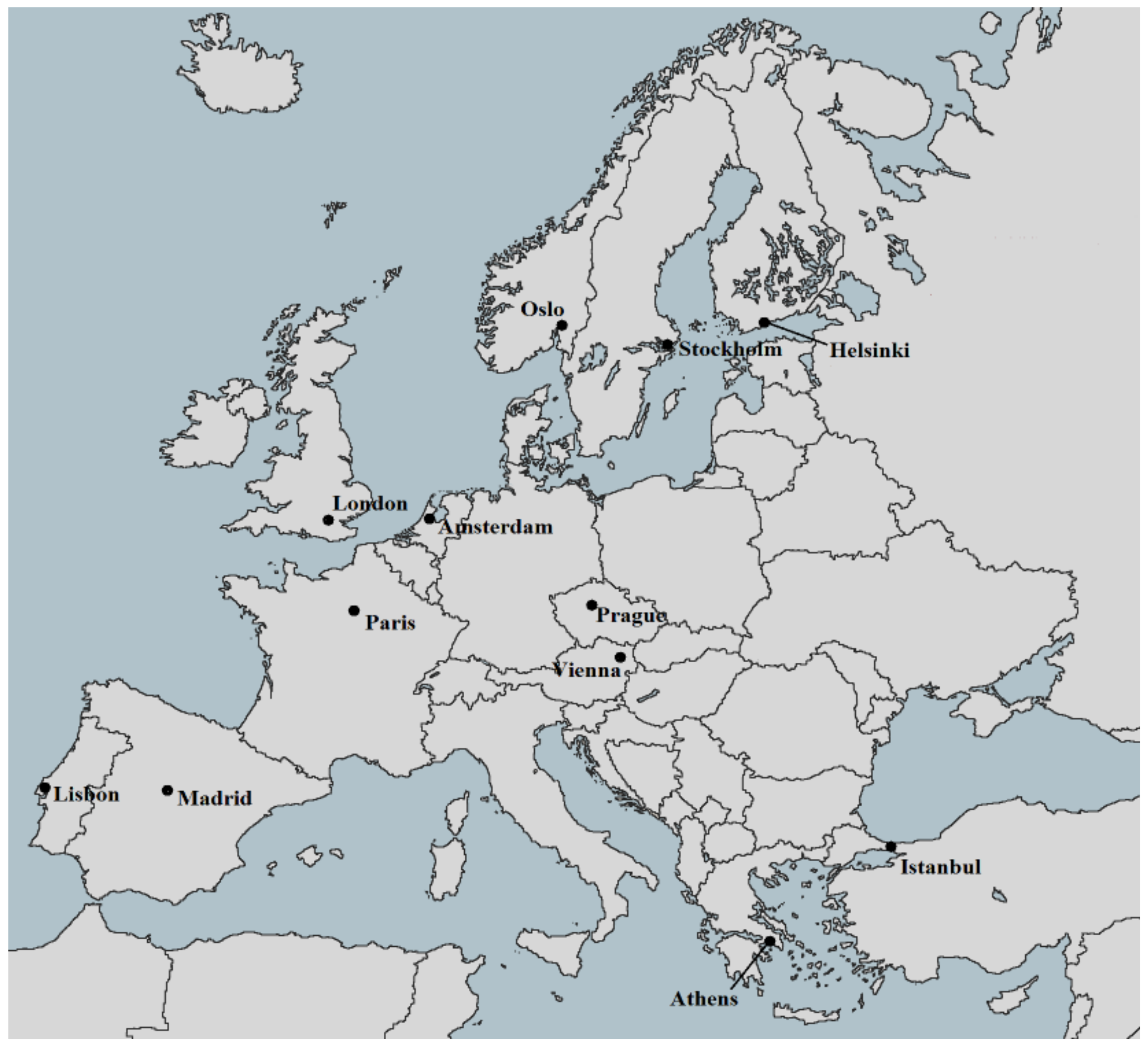
Based on the criteria described above, a total of 23 stations, distributed in 12 different European cities, were selected. Figure 1 presents the cities studied in this work and their location on the continent. The selection did not cover all available possibilities existing across Europe. However, it included a big distribution throughout the continent and regions with different conditions (geography, meteorology, etc.).
2.2. Sample Collection
Sample collection included PM2.5 and PM10 hourly concentrations, in µg/m3, for the selected stations, during the respective study period. Meteorological data (temperature, wind direction, wind speed, relative humidity and air pressure) were also collected from the station in Silivri (Istanbul). These data were obtained from different sources at European, national, and municipal levels. Table 1 presents the data sources for each city.
Table 2 summarizes information about the type, geographical locations (in Decimal Degrees Coordinates and Altitude), and the sampling period of all selected stations. Station ID was defined according to a XXYYZZ code, where XX refers to the station name, YY refers to the station type, and ZZ refers to the country code.
The criteria applied to exclude invalid PM concentration values was the following:
- (a)
- Negative concentration values were excluded;
- (b)
- Upper outliers (values 1.5 times above the 3rd quartile of each station’s hourly data) were excluded.
All the stations considered in this study presented data efficiency above 75% for the correspondent study period, for both PM2.5 and PM10 concentrations.
In Europe, the method for determining the PM concentrations at each station must be in accordance with the legislated standard gravimetric method (EN 14907:2005 for PM2.5 concentrations and EN 12341:1999 for PM10 concentrations), which validates the comparisons made in this study.
2.3. Temporal and Spatial Analysis
In this work, PM concentrations for different types of sites around Europe were compared to evaluate trends and behaviors in locations with different characteristics. Sites were organized according to their classification and different parameters were calculated and analyzed with Microsoft Excel + Visual Basic for Applications (VBA). The average annual, monthly, and daily values were calculated from the validated hourly data. In this analysis, the study period considered for Silivri (Istanbul) went from 2013 to 2017, despite its different sampling period (2013–2018).
To evaluate the overall temporal trends observed at the selected sites, linear regression was applied to their annual average concentration values. The variability of the profiles was evaluated according to their standard deviation (σ) values (Equation (1)):
where xi refers to the concentration values at a specific time (i), refers to the respective average value, and n is the size of the data set.
2.4. Statistical Model
In this study, a statistical model using Artificial Neural Networks (ANN) defined by Genetic Algorithm (GA) was applied (through MATLAB software, R2014a, MathWorks, Natick, MA, USA) to simulate and evaluate the combined effect of different variables on PM2.5 levels at the urban centre site SIUCTR (Istanbul), which presented the second highest PM2.5 concentrations between the selected sites. The selection of this station was also based on the availability of meteorological data needed to apply the model.
2.4.1. Artificial Neural Networks
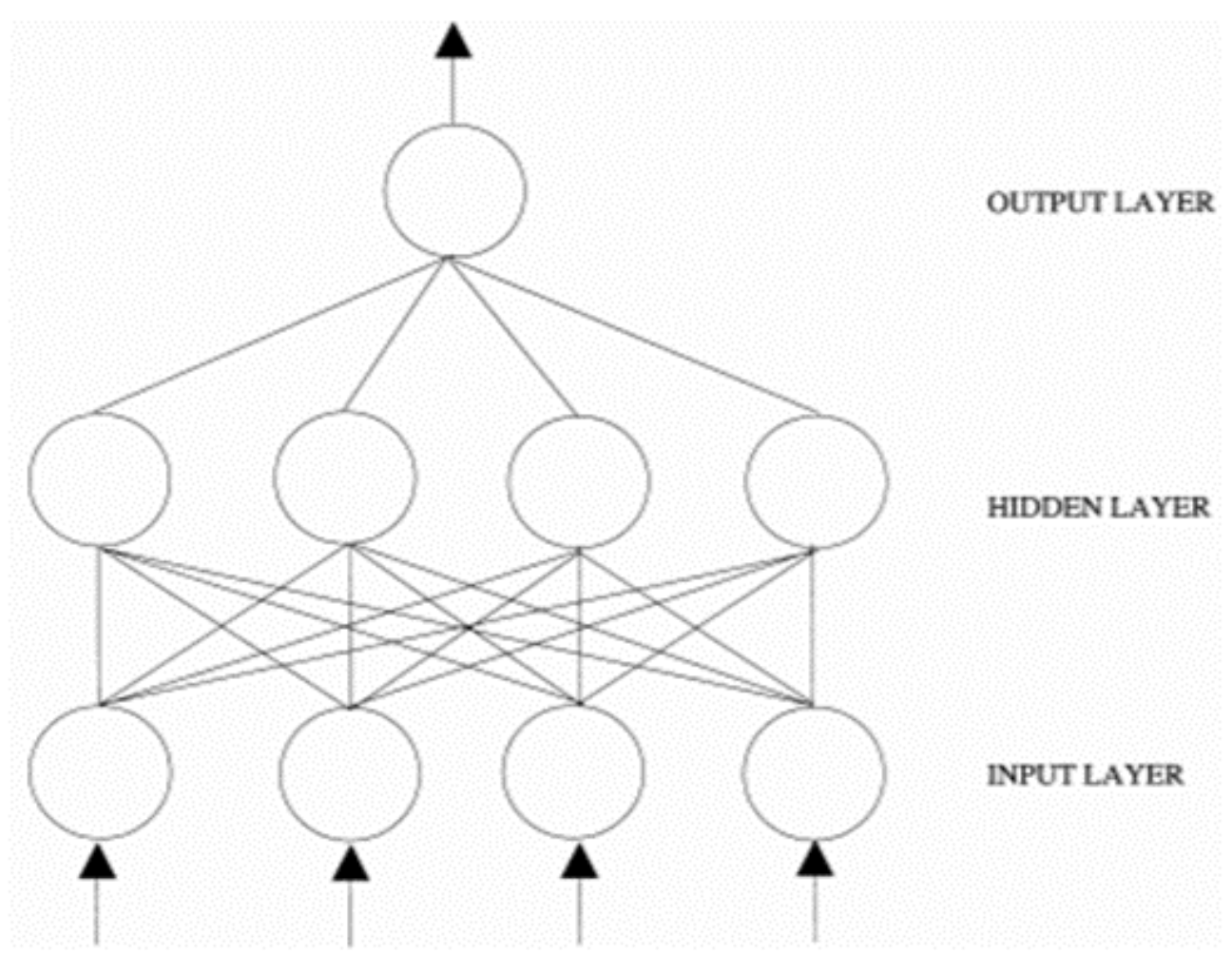
ANN are nonlinear models inserted in the field of Machine Learning used to perform complex calculations. This model is based on the behavior of the human brain. The human brain is composed, learns, and works through numerous neurons strongly interconnected between them. In the same way, ANN are computational methods that use a large set of elementary computational units (artificial neurons). Figure 2 presents a representative scheme of a possible ANN structure.
In ANN, a neuron can apply a local transformation (referred to as the activation function) to an input, providing an output signal. Besides the neurons, an ANN is constituted by the connection pattern among the neurons (structure or architecture of the network) and by the process used for training the neural network (learning algorithm). The structure of the network is defined by the way these neurons are distributed in layers (input, hidden, and output layers) and connected by synapses (each one carrying a weight/strength value, defined iteratively by the learning rule, according to the importance of input source). The neural network works to obtain valid outputs from the inputs [14,15,16,17,18].
2.4.2. Genetic Algorithms
GA are used to solve optimisation and search problems and are based on evolutionary biology. These algorithms encode a potential solution to a specific problem by iteratively modifying an initial randomly defined population of candidate solutions, tested against the objective/fitness function, and “evolving” them over successive generations toward an optimal solution. At each step, subsequent generations evolve from the previous using three rules: (i) selection of the fittest individuals (called parents) created in each generation, which will contribute to the population at the next generation; (ii) crossover of two parents to produce new solutions (called children) for the next generation; and (iii) mutation that applies random changes to individual parents to generate more new solutions [19,20,21,22].
2.4.3. Model Structure
The model applied in this study was structured similarly as defined by Afonso and Pires (2017) [23] and can be characterised by the following equation:
where y is the output variable, net1 and net2 are the ANN models, xi refers to the exploratory variables, xd is the threshold variable, and v is the threshold value.
The data of the explanatory variables were used as inputs to develop the proposed statistical model. These variables were related to hourly PM10 concentrations, the hour of measurement, the month of measurement, and meteorological variables (temperature, wind direction, wind speed, relative humidity and air pressure) measured from January 2013 to December 2018. Values related to the hour of measurement (H), the month of measurement (M) and wind direction (WD) were converted trigonometrically (Equation (3)) before being used as inputs:
where Yi refers to the converted value of the variable, Xi refers to the initial value of the variable, and T refers to the period of the variable (24 h for hour of measurement, 12 for the month of measurement, and 360° for wind direction) The output variable was the hourly PM2.5 concentrations measured at the same time as the input.
In this study, GA were used to define the threshold variable and value, the number of hidden neurons in the ANN, the activation function in the hidden layer of the ANN, and to select the explanatory variables to be used in each ANN model for three separate sets of time series (2013–2014; 2015–2016; 2017–2018). The specifications used in the determination of the model were defined as described by Afonso and Pires [23].
2.4.4. Model Performance Evaluation
The performance of the obtained models was evaluated using the following metrics: Mean Absolute Error (MAE), Mean Bias Error (MBE), Coefficient of Determination (R2), Root Mean Square Error (RMSE), and Index of Agreement of second-order (d2). MAE and RMSE are very common scale-dependent parameters, which measure the average magnitude of the error in a set of predictions [24]. If the positive/negative signs of the error are considered, MAE becomes MBE, which measures the average model bias. R2 translates the level of variance in the dependent variable that is predictable from the independent variable, while d2 measures the degree to which the model predictions are exact matches with no proportionality [24,25]. These parameters are calculated using the following equations:
where Oj refers to the observed values, is the mean of the observed values, Pj refers to the predicted values, and n is the size of the data set.
3. Results and Discussion
3.1. Behavior of PM2.5 Concentrations
3.1.1. Analysis of the Study Period
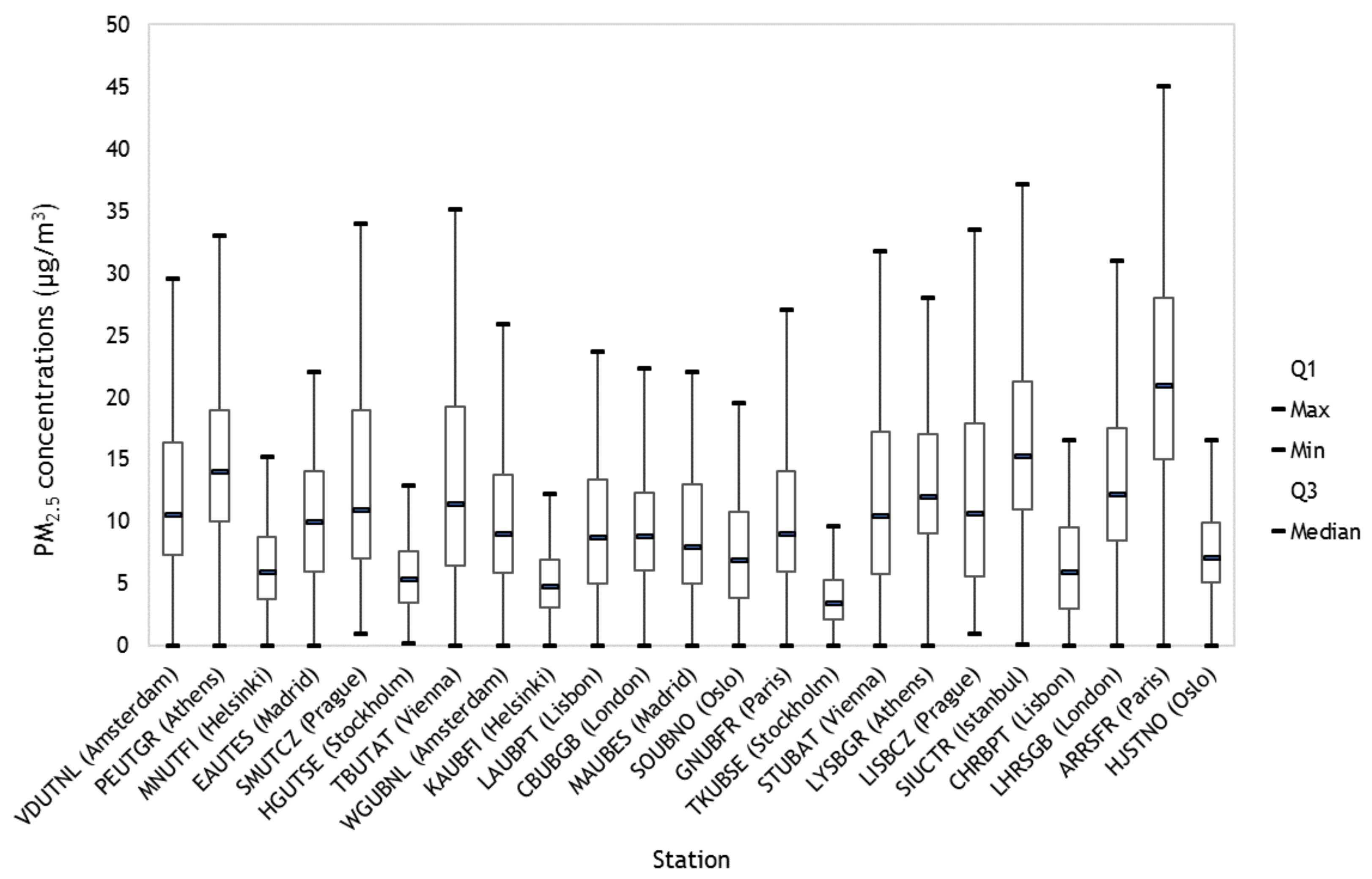
Figure 3 presents the distribution of PM2.5 concentrations during the study period of each selected site.
Different levels and ranges of PM2.5 concentrations were observed between the selected sites. Median concentration values ranged from 3.5 µg/m3 at TKUBSE (Stockholm) to 21.0 µg/m3 at ARRSFR (Paris). In general, higher levels of PM2.5 concentrations were observed at traffic-related sites, when compared to background sites. This behavior is commonly presented in a variety of studies related to PM levels in different environments, mainly due to the strong influence of traffic in PM emissions [12,26,27,28]. Another important observation is the lower PM2.5 levels at sites allocated in northern European cities (Helsinki, Stockholm and Oslo) when compared with other sites. Significant levels of concentration were observed at sites located in the Mediterranean area, especially those in Athens and Istanbul (south-eastern Europe). One of the reasons that can partially contribute to this behavior is the intense Saharan dust advection and deposition episodes that affect this area [29,30,31]. This phenomenon is considered an important source of dust particles, and it is responsible for significant increases of ambient PM concentrations in the Mediterranean area. According to the Air Quality Expert Group [32], high PM2.5 concentrations in the United Kingdom are partially associated with air transported from continental Europe, which may have had its impact on the selected sites located in London. Eeftens et al. [2] and EEA [11] analyzed the spatial variation of PM2.5 concentrations across Europe between 2008 and 2011 and during 2016, respectively. In these studies, the observed behavior was similar to the one found in this work, with lower PM2.5 values also happening in Northern Europe and the highest in Southern and Eastern Europe.
3.1.2. Annual Profiles
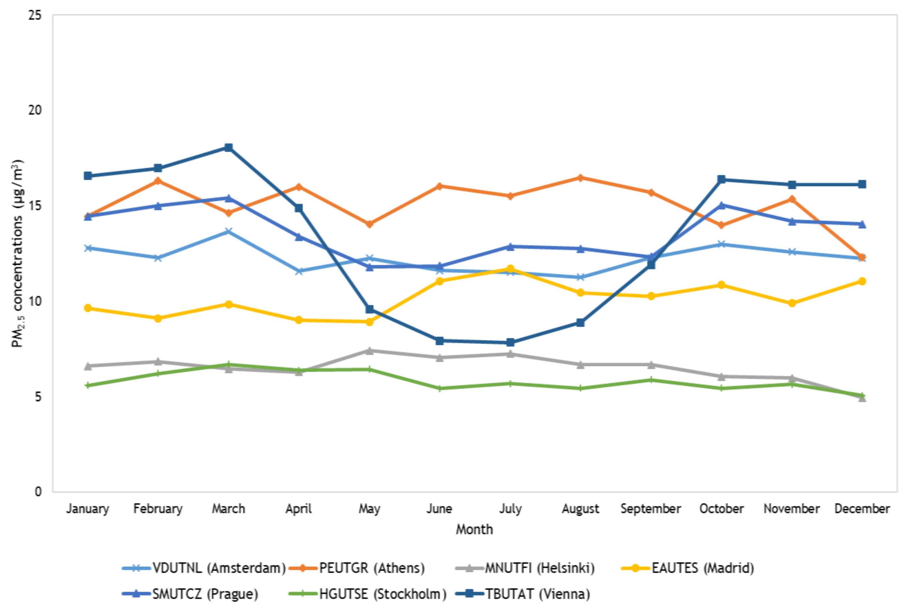
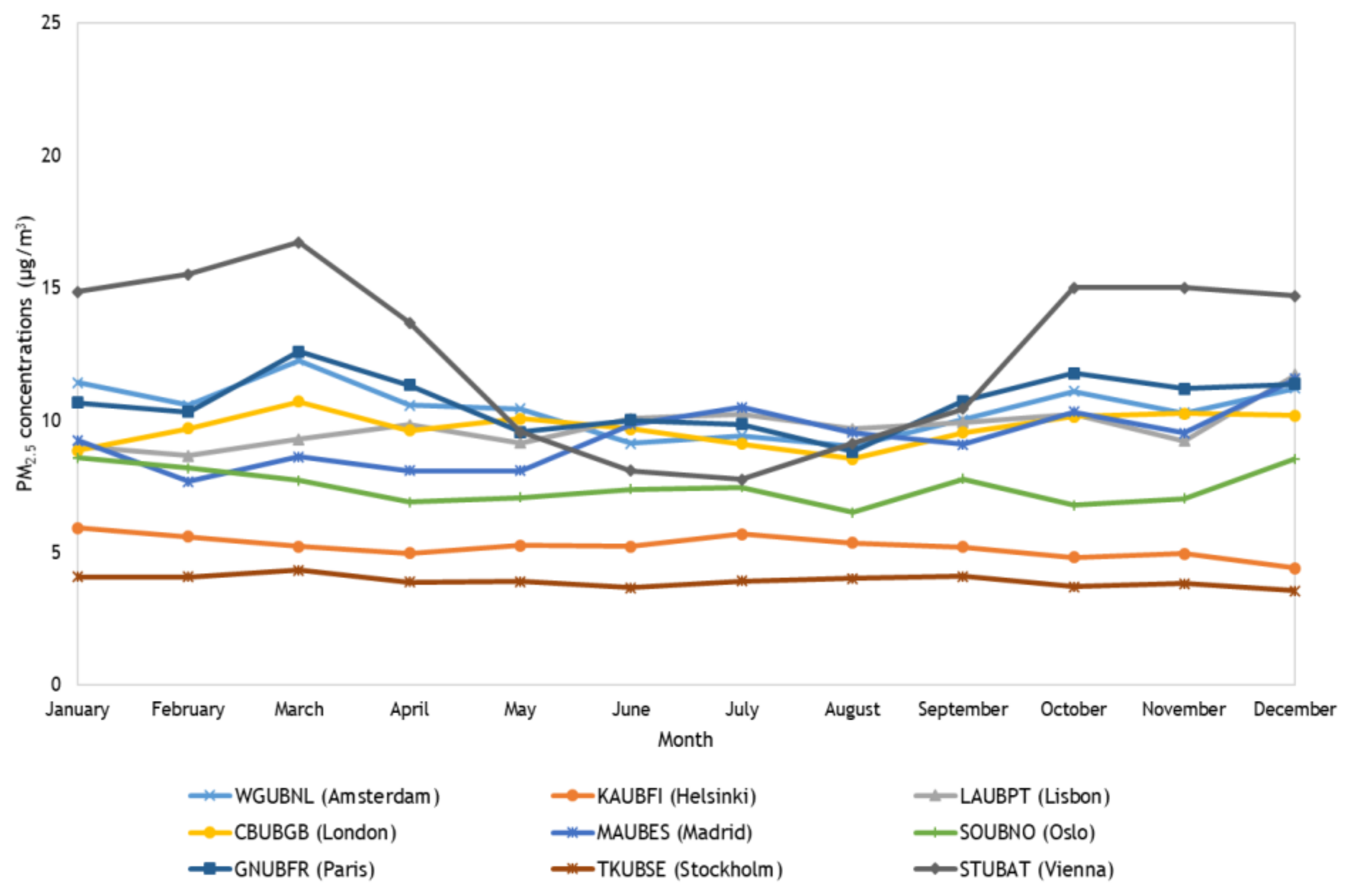
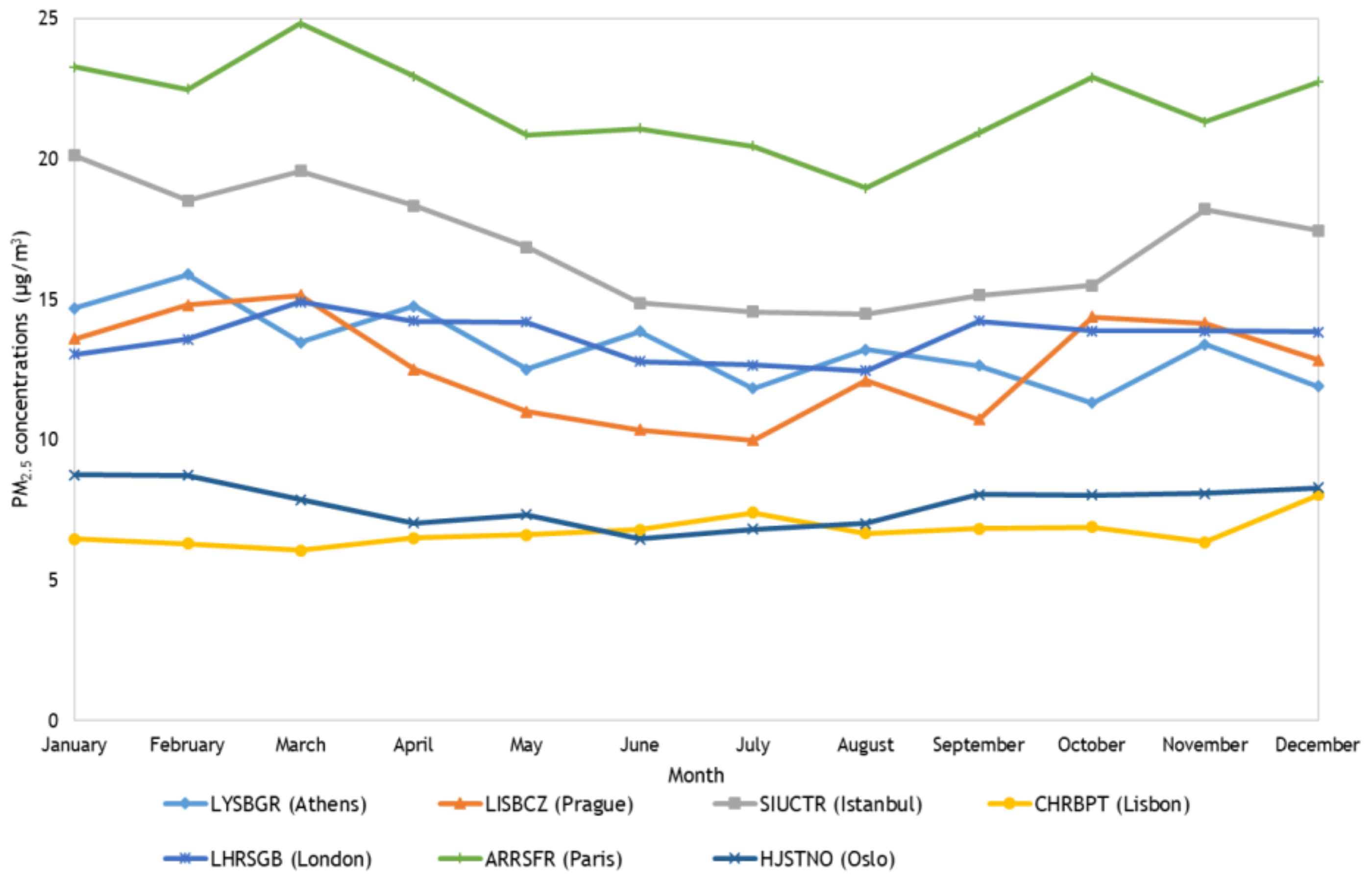
Figure 4, Figure 5 and Figure 6 present the annual average profiles of PM2.5 concentrations at the selected sites.
Different annual profiles of PM2.5 concentrations were observed at the selected sites. Seasonal behaviors are influenced by the combination of the diverse PM2.5 emission sources (e.g., industry, traffic, re-suspended dust) and factors like the meteorology, geography or economy. SMUTCZ (Prague) and, especially, TBUTAT (Vienna) were the urban traffic sites (Figure 4), where a stronger variability between months was observed (σ = 1.27 µg/m3 and 3.91 µg/m3, respectively). At these sites, significantly higher PM2.5 levels occurred during autumn and winter. This behavior is often associated with higher levels of combustion for central heating (domestic and industrial) and stronger thermal inversion conditions, which cause an accumulation of air pollutants in the lower layers of the atmosphere and are much stronger and frequent in colder months [33,34,35,36]. At both sites, a well-defined U-shaped profile is even observed during the period from March to October. Analyzing the different profiles, the variability, and behavior observed at the city of Vienna (Austria) stood out from the rest of the sites. According to Stadt Wien [37] (a Vienna environmental report), significantly higher levels in Vienna during winter can additionally be caused by stronger and adverse transport conditions of precursor pollutants (NOx, SO2, and NH3) over large distances. The same source informs that these transport conditions have a strong contribution on PM levels in Vienna (contribution of supra-regional sources were estimated to be approximately 75%, a much higher contribution compared to the 25% attributed to Vienna’s local sources). Despite the weak variability observed at VDUTNL (Amsterdam) and HGUTSE (Stockholm) sites (σ = 0.69 µg/m3 and 0.50 µg/m3, respectively), higher PM2.5 levels also happened during colder months at both sites, decreasing during spring and summer. This pattern is commonly presented in a variety of studies related to PM2.5 seasonality [6,38,39,40,41,42]. On the other hand, higher concentrations during summer were observed at MNUTFI (Helsinki) (σ = 0.66 µg/m3). As reported by some authors, a possible reason for this behavior is the stronger photochemical activity during higher temperatures, which contributes to the formation of secondary PM particles [38,43]. Biogenic emissions, which are higher in warmer seasons, can also have a significant impact on PM2.5 levels during that season [44,45,46,47]. In addition, the drier soils during warm months, together with strong winds, generate more dust, which might also have a contribution to higher levels [39,48]. Compared to other sites, PM2.5 variability at PEUTGR (Athens) and EAUTES (Madrid) was significant (σ = 1.22 µg/m3 and 0.90 µg/m3, respectively). However, evident seasonality was not found at these sites, and higher values were observed in both cold and warm months.
Compared to urban traffic sites, a weaker variability was observed at the urban background sites. However, significant seasonal behaviors were still found in the annual profiles. The highest monthly variation between the urban background sites happened at STUBAT (Vienna) (σ = 3.12 µg/m3). A clear seasonal behavior was also found at the same site through a well-defined U-shaped profile from March to October and much higher PM2.5 levels during colder months. Significant variations were also observed at WGUBNL (Amsterdam) and GNUBFR (Paris) (σ = 0.93 µg/m3 and 1.00 µg/m3, respectively), as well as higher PM2.5 concentrations in autumn and winter. Despite some relevant monthly variations (σ = 1.08 µg/m3 and 0.76 µg/m3, respectively), a clear seasonal behavior was not found at MAUBES (Madrid) and LAUBPT (Lisbon) sites. At KAUBFI (Helsinki), CBUBGB (London), SOUBNO (Oslo), and TKUBSE (Stockholm), weak monthly variations (σ = 0.39 µg/m3, 0.60 µg/m3, 0.65 µg/m3 and 0.21 µg/m3, respectively) and weak seasonality were observed.
Strong monthly variations were also observed at the suburban background site of LISBCZ (Prague), urban centre site of SIUCTR (Istanbul) and roadside site of ARRSFR (Paris) (σ = 1.81 µg/m3, 2.01 µg/m3 and 1.57 µg/m3, respectively). At these sites, a U-shaped profile was observed during spring and summer, with higher PM2.5 levels happening during autumn and winter. In comparison, weaker variations (σ = 0.75 µg/m3 and 0.76 µg/m3, respectively) were observed at the roadside site of LHRSGB (London) and suburban traffic site of HJSTNO (Oslo). Similar seasonal behaviors were found at these sites, with decreasing PM2.5 levels in spring and generally higher values happening in colder months. In the case of the suburban background site of LYSBGR (Athens), a clear seasonal behavior was not observed despite some relevant monthly variations (σ = 1.35 µg/m3). At the rural background site of CHRBPT (Lisbon), monthly variation (σ = 0.53 µg/m3) and seasonal behavior were not evident.
The PM2.5 annual profiles of Athens, Madrid and Lisbon (cities located in the Mediterranean area) exhibited high PM2.5 values during summer. This strengthens the idea of the influence and impact of Saharan dust episodes, which are usually more frequent in summer and highly affect the Mediterranean area [29,30,31,48,49,50]. Kopanakis et al. [29] studied PM levels in the eastern Mediterranean area of Europe. In that study, higher PM levels were observed during the summer, with correlation to dust events. Querol et al. [31] evaluated the influence of African dust outbreaks (ADOs) in Barcelona, which were also more frequent during summer and spring, and stated that PM1-10 and PM2.5-10 during ADOs were, respectively, 43 and 46% higher compared to non-ADO days.
In terms of differences of seasonal trends between the types of sites, no clear pattern was found. Generally, sites located in the same city presented similar annual behaviors, despite the type of environment in which they were located, which indicates that the geographic location in Europe has a big influence on these behaviors. In terms of general spatial differences, sites located in southern Europe presented weaker seasonal patterns, except at SIUCTR (Istanbul), while those located in northern and, especially, central Europe showed a stronger tendency to exhibit a seasonal pattern of higher PM2.5 levels during cold months.
3.1.3. Daily Profiles
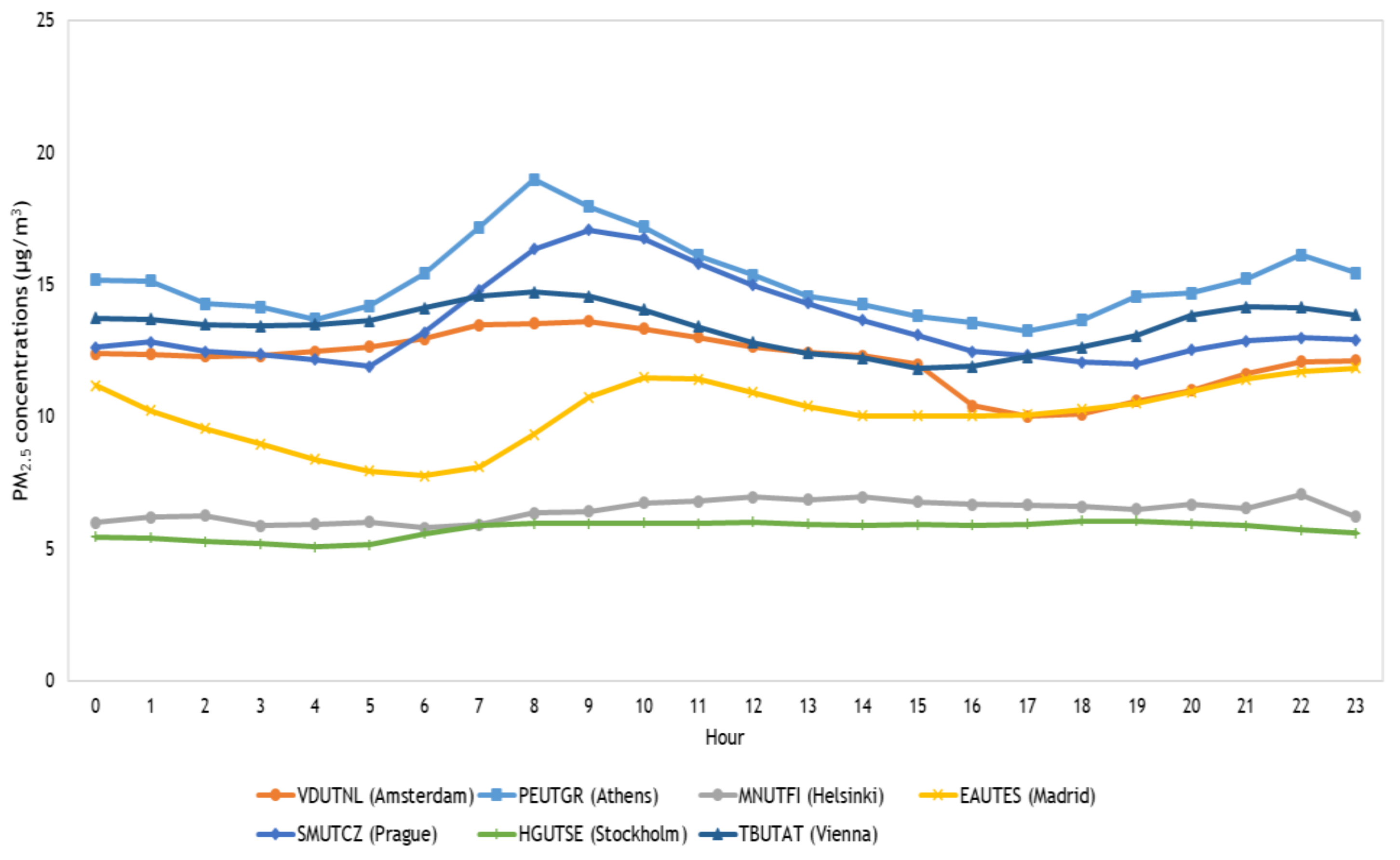
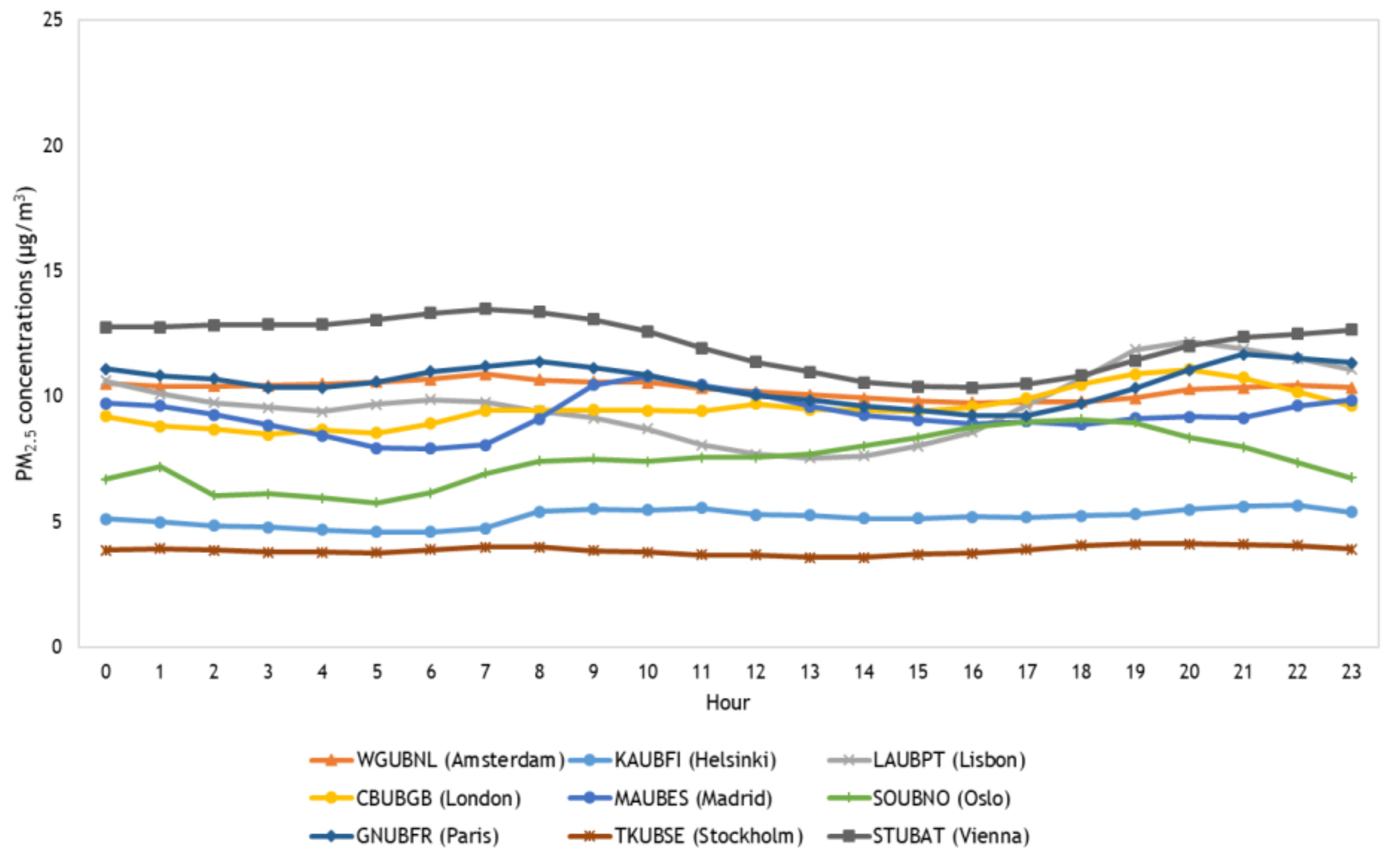
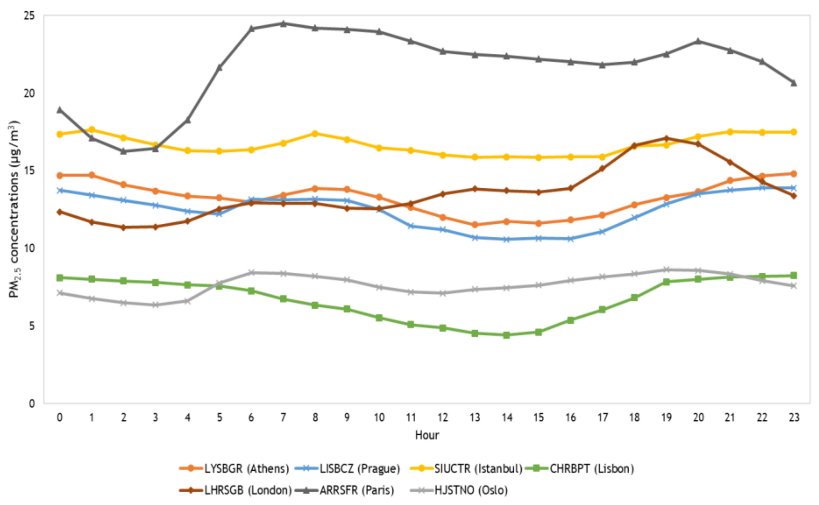
Figure 7, Figure 8 and Figure 9 present the daily average profiles of PM2.5 concentrations at the selected sites.
PM2.5 concentrations are also daily affected by their sources and related parameters like climate and meteorology, which lead to different diurnal behaviors in different regions. Relevant daily behaviors of PM2.5 concentrations were observed at the urban traffic sites. The strongest diurnal variability in urban traffic sites was observed at PEUTGR (Athens), EAUTES (Madrid) and SMUTCZ (Prague) sites (σ = 1.47 µg/m3, 1.21 µg/m3 and 1.59 µg/m3, respectively), especially during morning rush hours, where significant increases were observed. At these sites, decreasing PM2.5 values happened after morning rush hours until afternoon and during late night, and increasing values happened around morning and late rush hours. This pattern was also observed at TBUTAT (Vienna) and VDUTNL (Amsterdam), despite the lower variability (σ=0.85 µg/m3 and 1.05 µg/m3, respectively). This behavior is commonly stated in a variety of studies about diurnal variations of PM2.5 concentrations in different locations [6,40,51,52]. Increases of PM levels during the night period can be associated with more frequent temperature inversions and boundary layer dynamics related to that period [38,51,53,54]. In the case of MNUTFI (Helsinki) and HGUTSE (Stockholm), highly stable PM2.5 diurnal concentrations were observed (σ = 0.39 µg/m3 and 0.31 µg/m3, respectively).
The most significant diurnal variations of PM2.5 concentrations at urban background sites were observed at LAUBPT (Lisbon), SOUBNO (Oslo), and STUBAT (Vienna) sites (σ = 1.38 µg/m3, 1.01 µg/m3 and 1.04 µg/m3, respectively). Increasing levels from morning/noon until late afternoon were observed at SOUBNO (Oslo), CBUBGB (London), and LAUBPT (Lisbon). This behavior can be linked to higher dynamic human activities and higher levels of dust resuspension during that period of the day [5,54]. On the other hand, a continuous decrease during the same period was observed at GNUBFR (Paris) and STUBAT (Vienna). The more easily identifiable influence of rush hours among the urban background sites was found at MAUBES (Madrid). At this site, PM2.5 values increased significantly during morning rush hours, decreasing continuously afterwards. High diurnal stability was found at WGUBNL (Amsterdam), KAUBFI (Helsinki), and TKUBSE (Stockholm) (σ = 0.32 µg/m3, 0.32 µg/m3 and 0.16 µg/m3, respectively).
Strong variability of PM2.5 was also found at the roadside sites of LHRSGB (London) and ARRSFR (Paris) (σ = 1.64 µg/m3 and 2.47 µg/m3, respectively). In the case of LHRSGB (London), a strong peak was observed during the afternoon. At ARRSFR (Paris), a U-shaped profile was observed from 20 h to 6 h. Some diurnal variations were also observed at the suburban background sites of LYSBGR (Athens) and LISBCZ (Prague) and at the rural background site of CHRBPT (Lisbon) (σ = 1.04 µg/m3, σ = 1.14 µg/m3 and 1.36 µg/m3, respectively). Very similar behaviors were found at the suburban background sites of LYSBGR (Athens) and LISBCZ (Prague), with increases of PM2.5 concentrations being observed during rush hours, decreasing afterwards. At the rural background site of CHRBPT (Lisbon), PM2.5 levels continuously decreased from 0 h to 14 h and increased during the rest of the period. Less variability of PM2.5 concentrations was observed at the urban centre site of SIUCTR (Istanbul) and suburban traffic site of HJSTNO (Oslo) (σ = 0.62 µg/m3 and 0.68 µg/m3, respectively). However, increasing PM2.5 levels during rush hours were found at both sites, decreasing afterwards.
As expected, rush hour influence on diurnal profiles of PM2.5 concentration was more noticeable at traffic-related sites than background sites. However, the highest PM2.5 concentrations at background sites were also observed during that period. Some differences were also found on a spatial level. Sites located in northern Europe, especially those in Helsinki and Stockholm, exhibited higher stability in their daily profile when compared to the rest of the sites.
3.2. Behavior of PM2.5/PM10 Ratios
3.2.1. Analysis of the Study Period
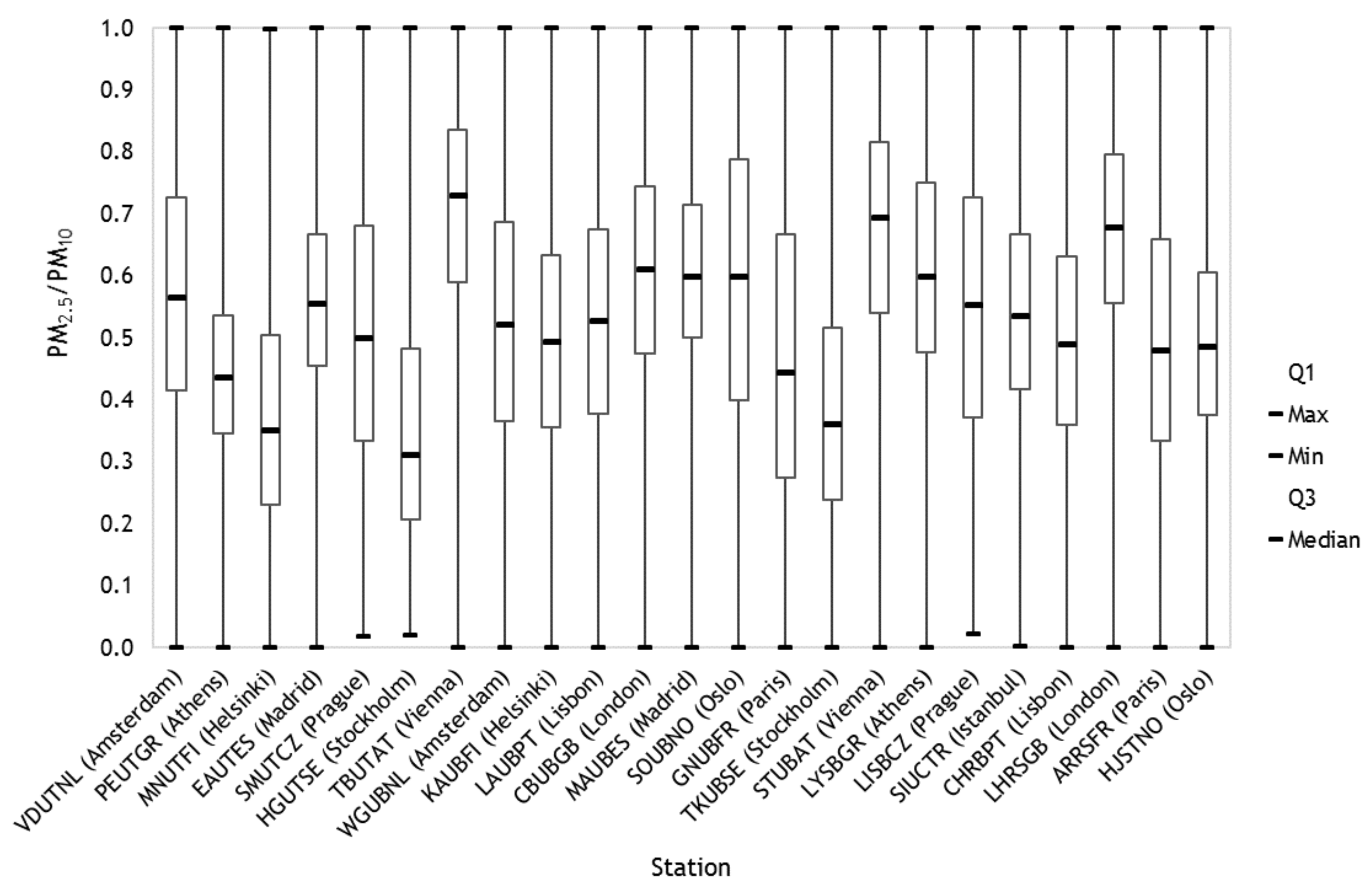
Figure 10 presents the distribution of the average PM2.5/PM10 ratio values at the selected sites.
Considering the variety of complex and changing PM sources and the factors that influence its values, it was expected that the PM2.5/PM10 ratio values would also show significant variations between sites. These results were in agreement with that, with a variety of levels and ranges of PM2.5/PM10 ratio values being observed at the selected sites. Median ratio values ranged from 0.31 at HGUTSE (Stockholm) to 0.73 at TBUTAT (Vienna).
At most sites, median ratio values were above 0.5, which indicates that the concentrations of fine particles, which can be located in deep regions of the respiratory system, tended to be higher than those of coarse particles. Munir [6] and Xu et al. [5] studied PM presence at different sites in Wuhan (China) (2013–2015) and UK (2010–2014), respectively. In both studies, the predominance of PM2.5 over coarse particles was stated. According to Munir [6], this can be partially attributed to fine particles being more persistent in the atmosphere than coarse particles.
Generally, PM2.5/PM10 ratios were slightly higher at background sites, which can be associated with higher levels of re-suspended road dust at traffic sites, which is a major contributor to higher PM10 concentrations and, therefore, lower PM2.5/PM10 values [5]. However, in the case of Amsterdam, London, Paris, and Vienna, higher values were observed at the respective traffic site than at the background site. This observation can be an indicator of a higher predominance of vehicular combustion emissions in these locations because fine particles (PM2.5) are more influenced by combustion sources than coarse particles (PM2.5–10) [6,26,55]. Querol et al. [28] compared PM characteristics, from 1998 to 2002, at different European regions and stated that the ratio was highly dependent on the type of site. In the same study, lower ratios were obtained at kerbside sites, while the values at regional background sites were generally higher, which differs from the results obtained in this work.
In terms of overall spatiality, the lowest PM2.5/PM10 values of the selected sites were found at sites located in northern Europe (specifically Helsinki and Stockholm), while no clear difference was observed between the rest of the continent.
3.2.2. Annual Profiles
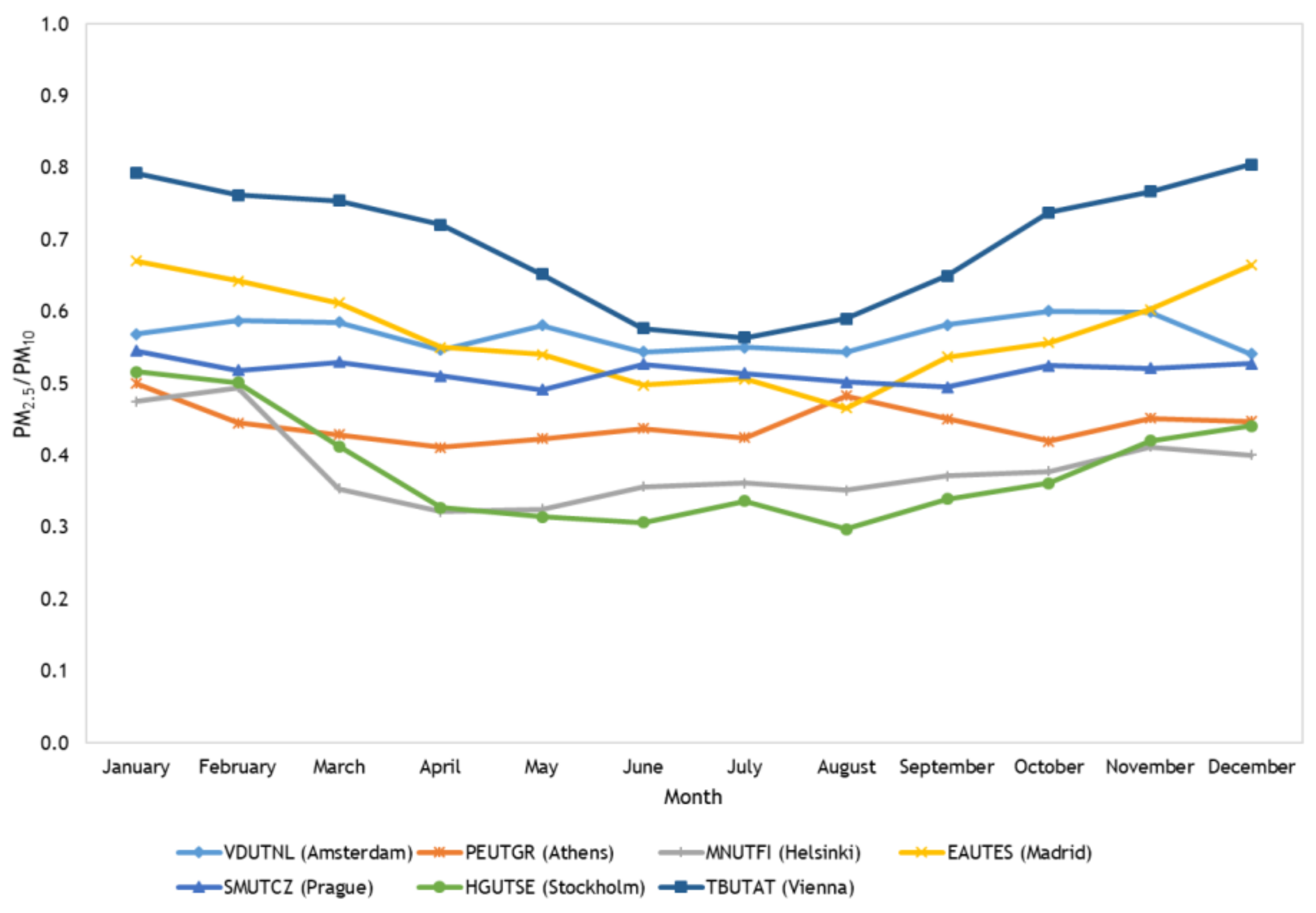
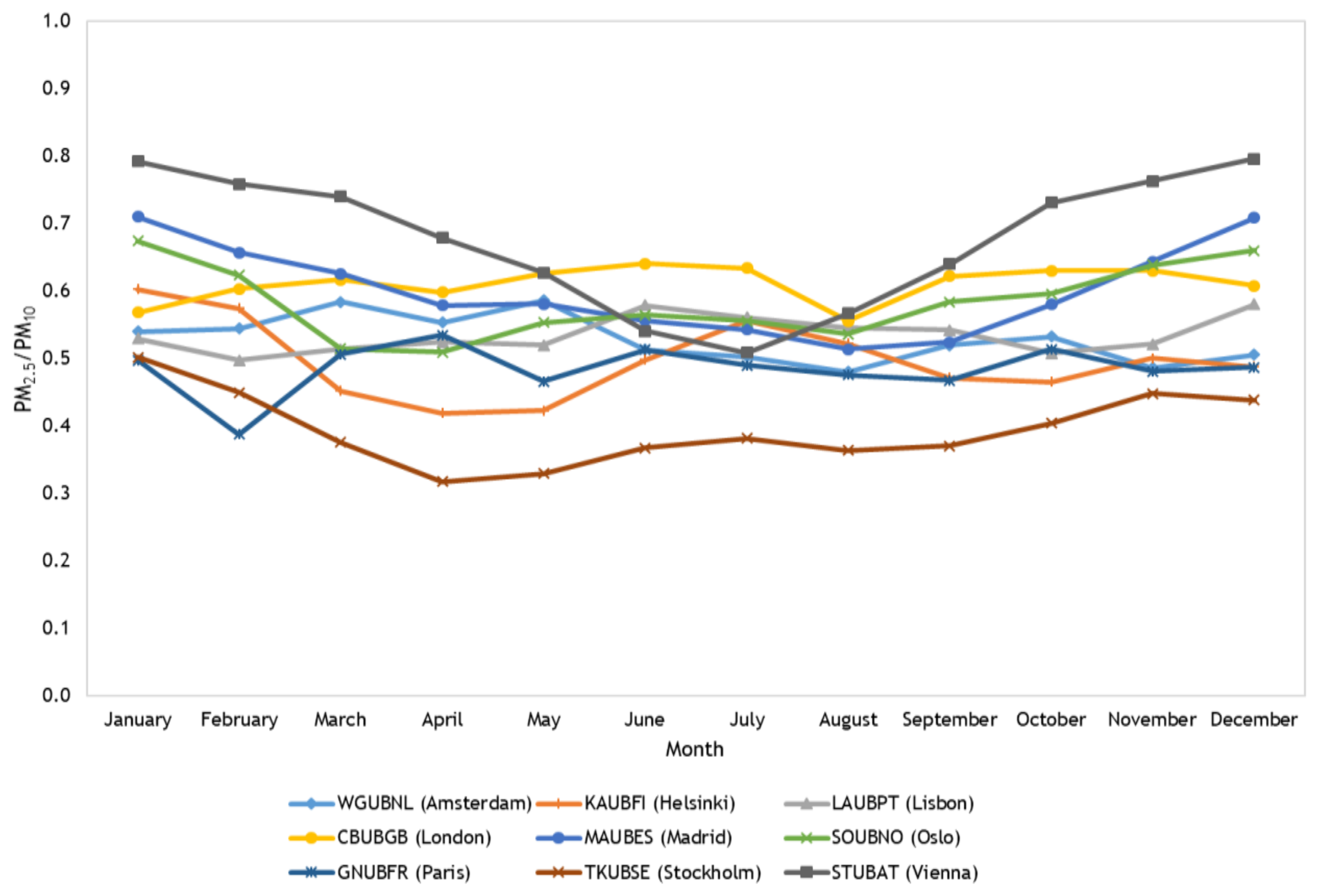
Figure 11, Figure 12 and Figure 13 present the annual average profiles of the PM2.5/PM10 ratio at the selected sites.
Different annual profiles of PM2.5/PM10 ratio were observed at the selected sites. Meteorological factors like temperature, wind speed, and precipitation have an important effect on PM concentrations and their ratios. These factors tend to vary a lot during a year, and so they have a big impact on the seasonality of the annual profiles. That tendency was also observed in the results obtained in this section.
EAUTES (Madrid), HGUTSE (Stockholm), and TBUTAT (Vienna) were the urban traffic sites where a stronger variability between months was observed (σ = 0.067, 0.075 and 0.087, respectively). Similar seasonal behavior was also observed at these sites, with a general decrease of the ratio happening during warmer months, increasing during the colder season. The same behavior was observed at MNUTFI (Helsinki), but with lower levels of variation (σ = 0.054), which was the most common pattern observed at the selected urban traffic sites. Some authors associate this behavior with: (i) higher usage of domestic and industrial heating (important sources of PM2.5) during the cold season; (ii) higher dust re-suspension (major contributor to higher PM10 levels) during the dry season; (iii) higher wind speed and precipitation and their negative effect on larger particles; and an (iv) increase of biogenic coarse PM during the warm season [5,6,26,43,56,57]. Munir [6] and Xu et al. [5] also identified generally higher levels during winter in their studies. However, a strong increase of the ratio during June and July was observed by Munir in the UK. Sorek-Hamer et al. [58] also evaluated the seasonality of the PM ratio in different global locations (France, Israel, Italy, and the USA) and observed ratio increases in Israel during the warm season. The study states that this tendency can be partially related to air transport events, which affect both PM fractions differently. VDUTNL (Amsterdam), PEUTGR (Athens), and SMUTCZ (Prague) were the urban traffic sites where less variability of PM2.5/PM10 ratios was observed (σ = 0.023, 0.026 and 0.016, respectively). However, slightly higher PM2.5/PM10 values during autumn and winter were also observed at VDUTNL (Amsterdam), while higher values were found in both cold and warm months at PEUTGR (Athens), SMUTCZ (Prague).
Comparing the monthly variability of PM2.5/PM10 values between urban traffic and urban background sites, no clear differences were found. The highest monthly variation of PM2.5/PM10 ratio of all selected sites was observed at STUBAT (Vienna) (σ = 0.096). A clear seasonality was also observed at this site, with continuously declining values happening in the first half of the year, increasing during the rest of the months. Monthly variations were also significant at KAUBFI (Helsinki), MAUBES (Madrid), SOUBNO (Oslo), and TKUBSE (Stockholm) (σ = 0.055, 0.064, 0.053 and 0.052, respectively). A strong decline of the ratios during winter and spring, increasing in summer, was found at KAUBFI (Helsinki) and MAUBES (Madrid). In the case of SOUBNO (Oslo) and TKUBSE (Stockholm), a similar seasonality was observed between them, with the profile declining from January to April and increasing almost continuously during the rest of the year. WGUBNL (Amsterdam), LAUBPT (Lisbon), CBUBGB (London), and GNUBFR (Paris) (σ = 0.033, 0.026, 0.025 and 0.035, respectively) were the urban background sites where less variability was found. Weak seasonal behaviors were observed at CBUBGB (London) and GNUBFR (Paris). Higher ratio values happened mainly during winter and spring at WGUBNL (Amsterdam) and during the summer at LAUBPT (Lisbon).
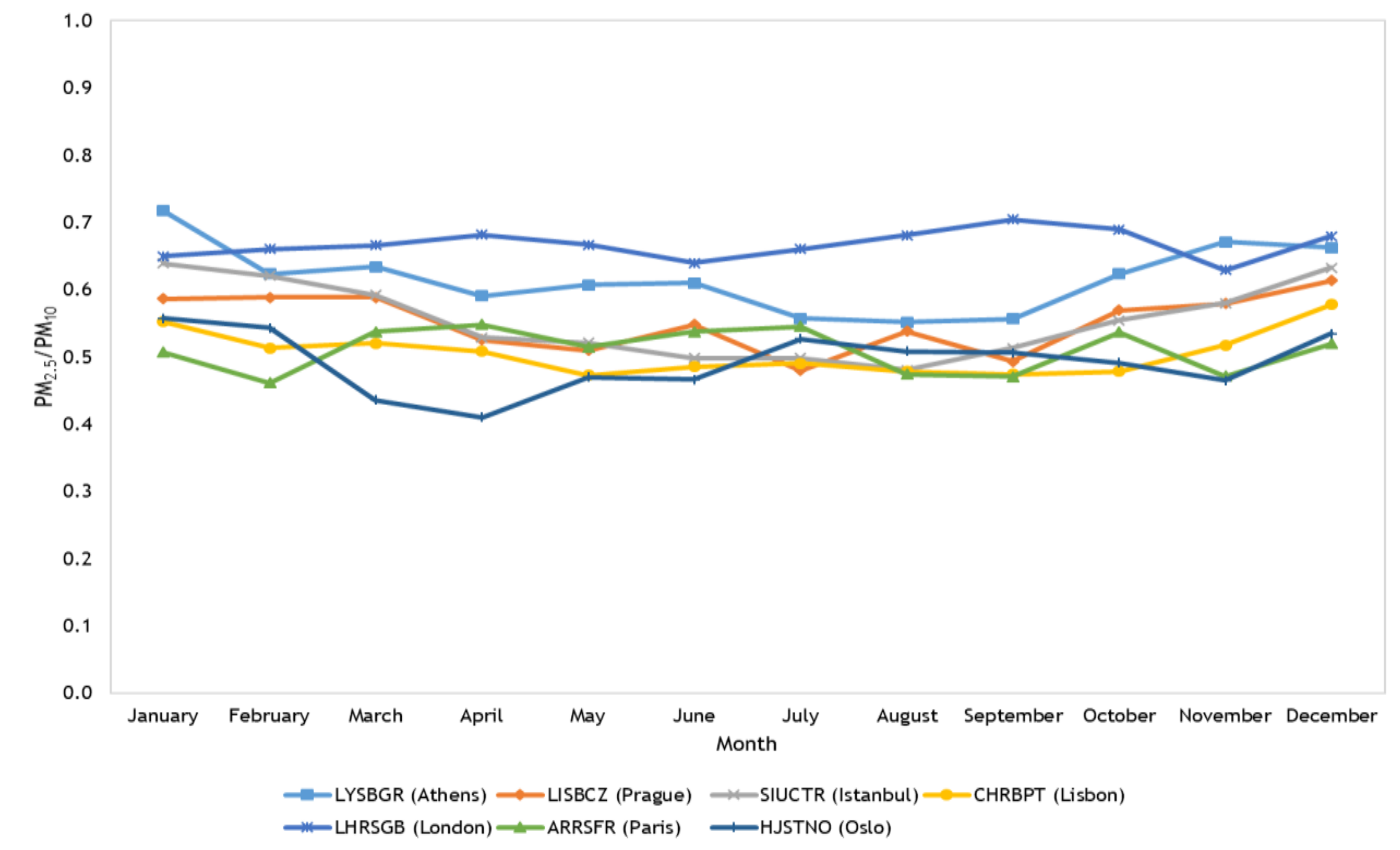
Significant seasonal variability was observed at the suburban background sites of LYSBGR (Athens) and LISBCZ (Prague), urban centre site of SIUCTR (Istanbul) and the suburban traffic site of HJSTNO (Oslo) (σ = 0.050, 0.043, 0.056 and 0.045, respectively). PM2.5/PM10 values were generally higher during autumn and winter at LYSBGR (Athens) and LISBCZ (Prague). Lower values happened during the spring at HJSTNO (Oslo). Continuously decreasing values from January to August, increasing during the rest of the months, happened at SIUCTR (Istanbul). Highly stable values were observed in the annual profile of the rural background site of CHRBPT (Lisbon) and at the roadside sites of LHRSGB (London) and ARRSFR (Paris). PM2.5/PM10 values were higher during the winter, slightly decreasing in warmer months at CHRBPT (Lisbon). Ratio values presented a weak seasonality at LHRSGB (London) and ARRSFR (Paris). In general, a slightly more evident seasonality was found at the selected background sites compared to traffic-related sites.
3.2.3. Daily Profiles
Figure 14, Figure 15 and Figure 16 present the daily average profiles of PM2.5/PM10 ratios at the selected sites.
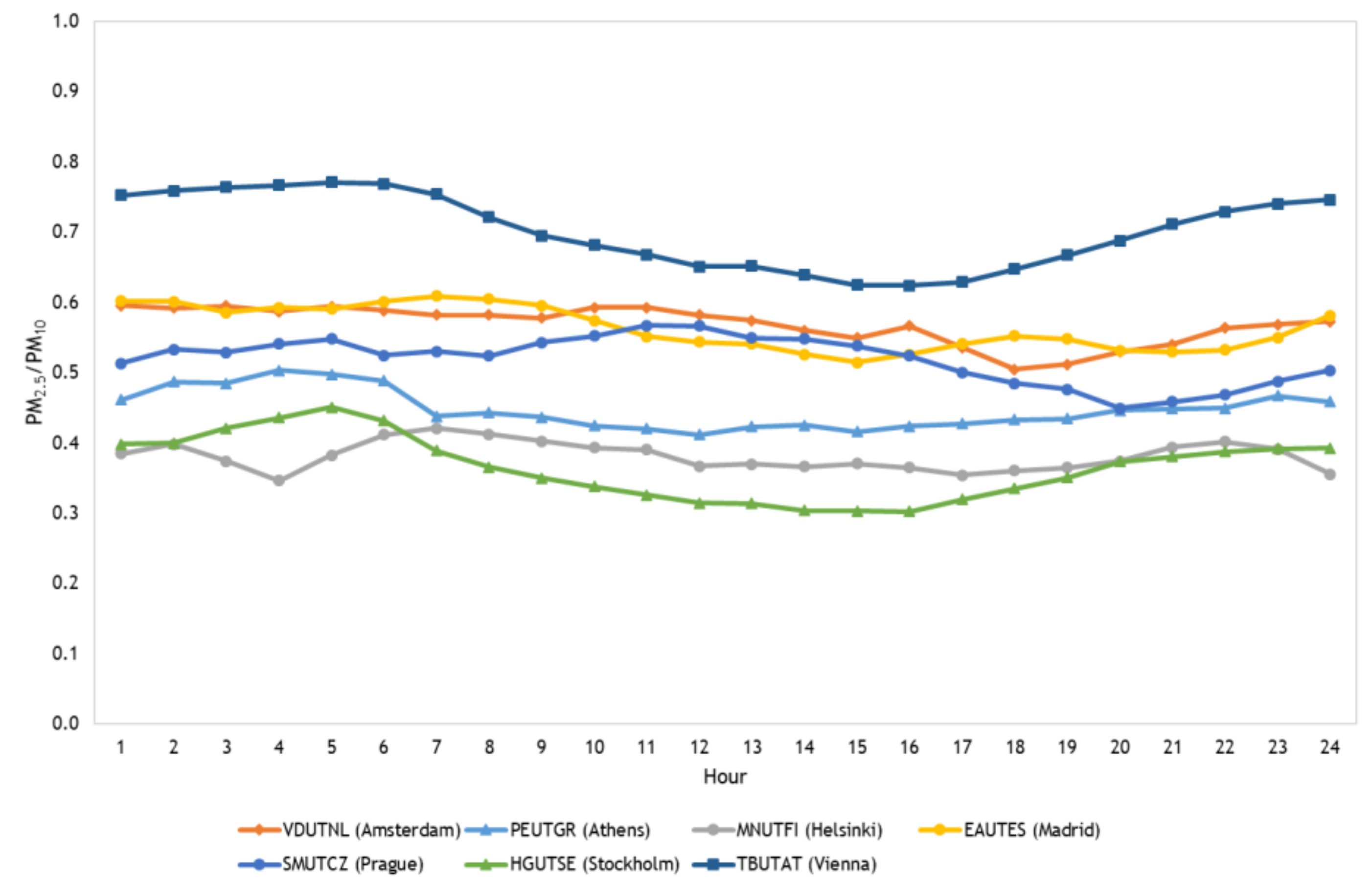
The variety of sources and factors that influence PM2.5/PM10 ratio values not only have their impact on a seasonal level but also on a diurnal level, as it is perceptible by the variations and behaviors of the daily profiles in this analysis. The urban traffic sites with stronger diurnal variations were HGUTSE (Stockholm) and TBUTAT (Vienna) (σ = 0.045 and 0.052, respectively). Similar and clear seasonality happened at these sites, with the ratio values strongly and continuously increasing during the night and decreasing during morning and afternoon. This was the most common pattern found in the analysis of the diurnal profiles in this work. This behavior was also stated in a variety of studies [5,6,55]. According to Xu et al. [5], this night-day difference can be associated with stronger temperature inversion during the night and stable atmospheric conditions favourable to the dry deposition of coarse particles and the accumulation of PM2.5 in the air. Significant diurnal variations also happened at EAUTES (Madrid) and SMUTCZ (Prague) (σ = 0.031 and 0.034, respectively). Ratio values were higher during the night/early morning and slightly increased during rush hours at EAUTES (Madrid). At SMUTCZ (Prague), those values were higher during the daytime, especially after morning rush hours. The urban traffic sites with higher stability were VDUTNL (Amsterdam), PEUTGR (Athens), and MNUTFI (Helsinki) (σ = 0.027, 0.027 and 0.020, respectively). At VDUTNL (Amsterdam) and PEUTGR (Athens), ratio values were higher during the night/early morning, declining during the daytime. Slight increases during rush hours were observed at MNUTFI (Helsinki). Increases of the ratio values during rush hours, as the one observed at EAUTES (Madrid) and MNUTFI (Helsinki), can be linked to the significant contribution by direct vehicular emissions during that period, which is stronger for PM2.5 than for coarse particles [5,6,26].
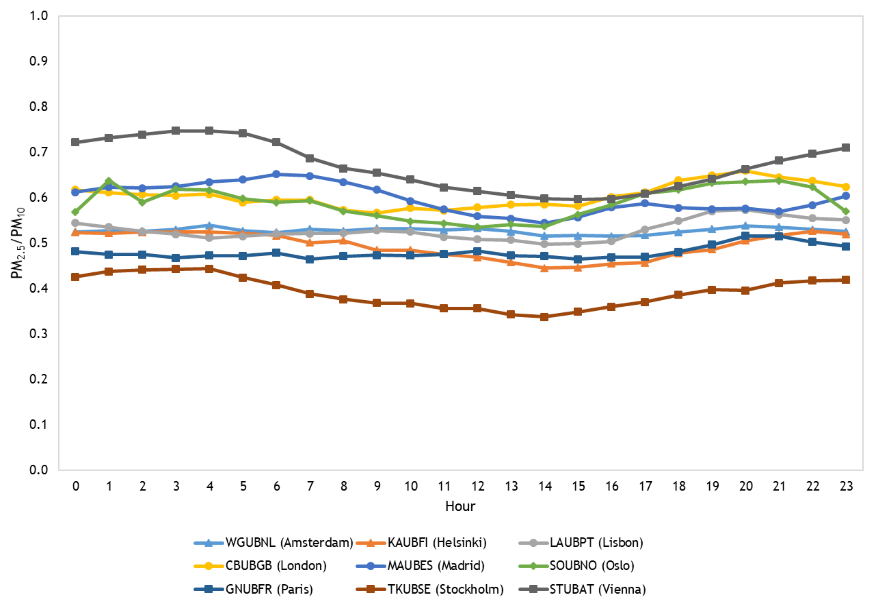
The urban background sites where a higher diurnal variability was observed were MAUBES (Madrid), SOUBNO (Oslo), TKUBSE (Stockholm) and, especially, STUBAT (Vienna) (σ = 0.032, 0.034, 0.034 and 0.054, respectively). In comparison, stable diurnal values were observed at KAUBFI (Helsinki) and CBUBGB (London) (σ = 0.028 and 0.026, respectively). Similar daily profiles were found at these sites, with higher/increasing ratio values happening during the night/early morning and having the opposite behavior during the daytime. The urban background sites with a higher ratio stability were WGUBNL (Amsterdam), LAUBPT (Lisbon) and GNUBFR (Paris) (σ = 0.006, 0.022, and 0.015, respectively). Increasing values during late afternoon happened at GNUBFR (Paris) and LAUBPT (Lisbon), while no clear seasonal behavior was observed at WGUBNL (Amsterdam).
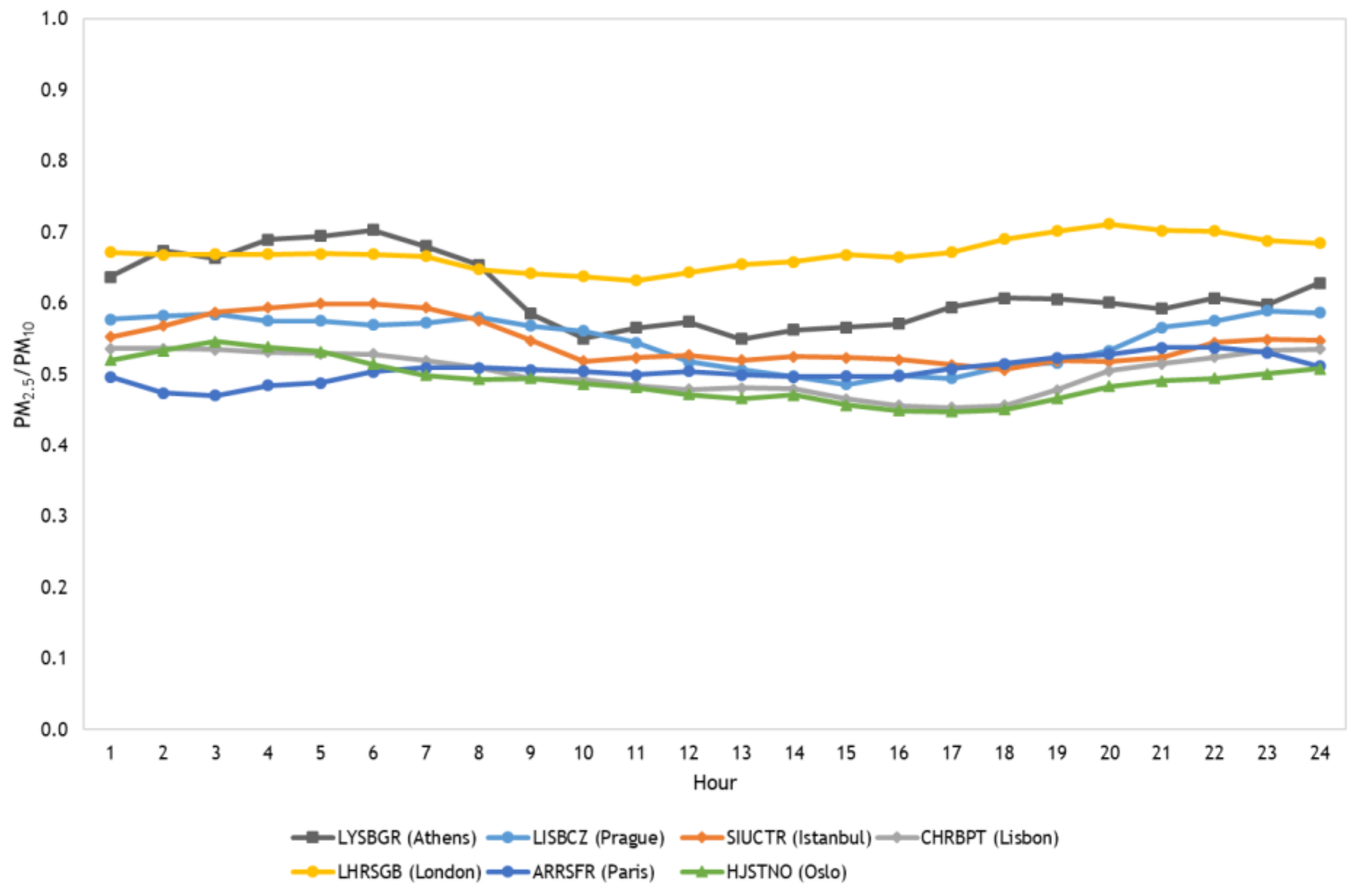
A strong diurnal variability was observed at the suburban background site of LYSBGR (Athens) (σ = 0.049). Significant diurnal variations were also found at the suburban background site of LISBCZ (Prague), urban centre site of SIUCTR (Istanbul), rural background site of CHRBPT (Lisbon), and suburban traffic site of HJSTNO (Oslo) (σ = 0.035, 0.031, 0.029, and 0.029). At these sites, higher and increasing ratio values happened during the night, decreasing during early morning and morning rush hours. Stronger decreases observed during rush hours, like the one at LYSBGR (Athens), can be influenced by the higher occurrence of re-suspended coarse road dust [5,6,26]. A weak diurnal variability was observed at the roadside sites of LHRSGB (London) and ARRSFR (Paris) (σ = 0.021 and 0.018, respectively). However, some diurnal behaviors were still found. Increasing ratio values happened during the day at LHRSGB (London). At ARRSFR (Paris), the ratio values were stable during morning and afternoon, oscillating during the night, with the highest values occurring during late rush hours.
When comparing overall diurnal variability values between traffic and background sites, those presented to be very similar. The most commonly observed pattern, with higher/increasing ratio values during the night-time and lower/decreasing values during the daytime, was more frequent in background sites. However, that tendency was also found in traffic-related sites.
3.3. Modelling of PM2.5 Concentrations
3.3.1. Statistical Models
The combination of ANN with GA allowed obtaining different threshold models for the three considered periods (2013–2014, 2015–2016, and 2017–2018). Table 3 presents the characteristics of the obtained models, in terms of explanatory variables, threshold variables and values, activation function (AF), and the number of hidden neurons (HN).
The obtained threshold models defined the month of measurement (M), RH and T as the variables that could set different regimes for PM2.5 concentrations. For the 2013–2014 period, the obtained model did not select the variables H and RH when M < 0.92 (January to April and August to December) and RH when M ≥ 0.92 (May to July). For the 2015–2016 period, the selected variables did not include M and WD when RH < 79.1% and M when RH ≥ 79.1%. For the 2017–2018 period, the selected variables included all the input variables when T < 11.2 °C and did not include M and RH when T ≥ 11.2 º C.
In terms of fitting performance, the model related to the 2017-2018 period presented the best results (MAE = 2.85 µg/m3; MBE = 0.03 µg/m3; R 2= 0.61; RMSE = 3.67 µg/m3; d2 = 0.87), followed by 2015–2016 (MAE = 2.98 µg/m3; MBE =-0.03 µg/m3; R2 =0.52; RMSE= 3.89 µg/m3; d2 = 0.83) and 2013–2014 (MAE = 3.56 µg/m3; MBE = -0.59 µg/m3; R2 = 0.42; RMSE= 4.64 µg/m3; d2 = 0.79). Despite the computational model being only applied to one station (due to the availability of meteorological data), the performance results show that the model can be an important tool in the analysis of the PM2.5 concentration behaviors at other sites. The relationships between PM2.5 concentrations and meteorological variables may be similar.
3.3.2. Combined Effects of Meteorological Variables and PM10 Concentrations on PM2.5 Concentrations
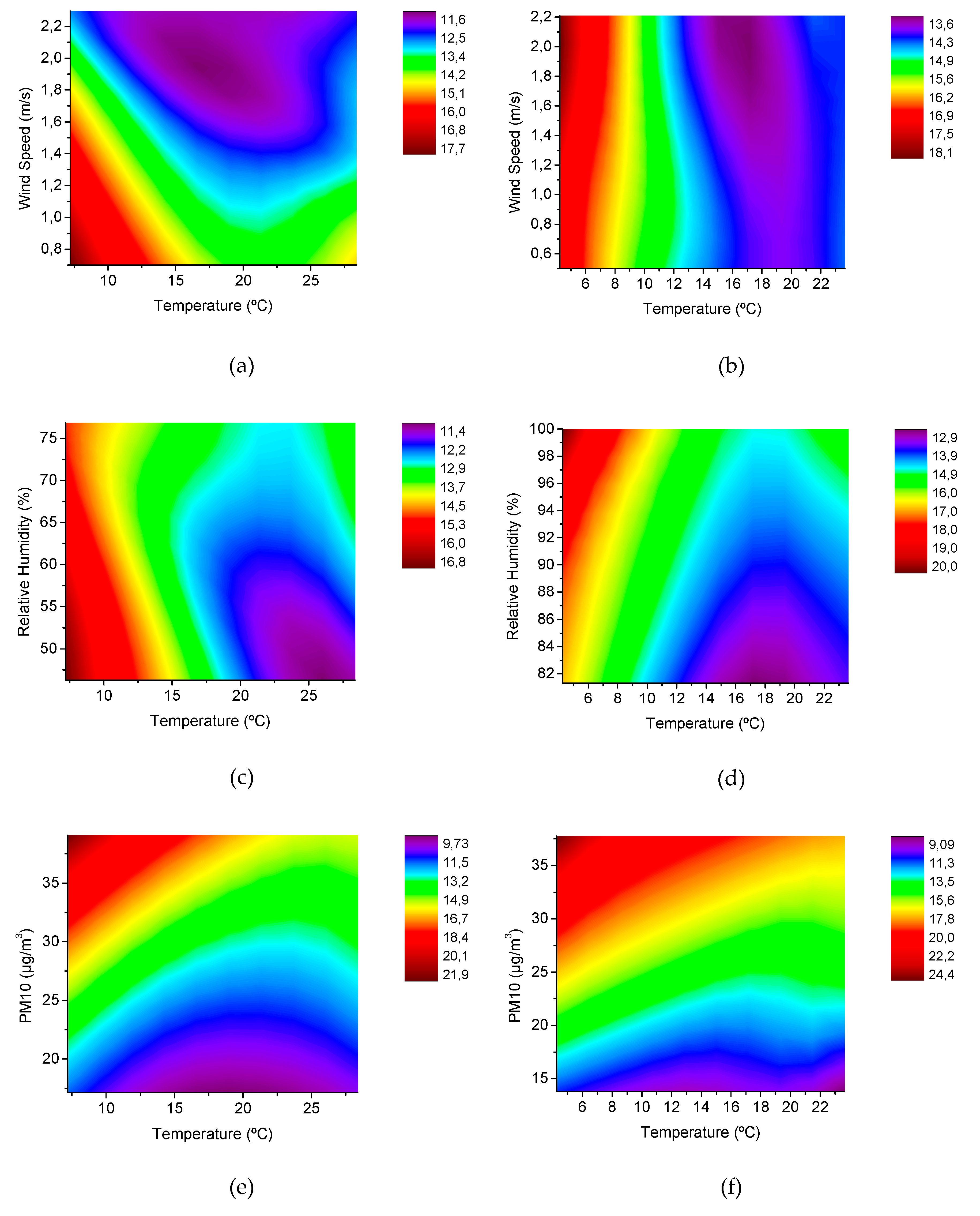
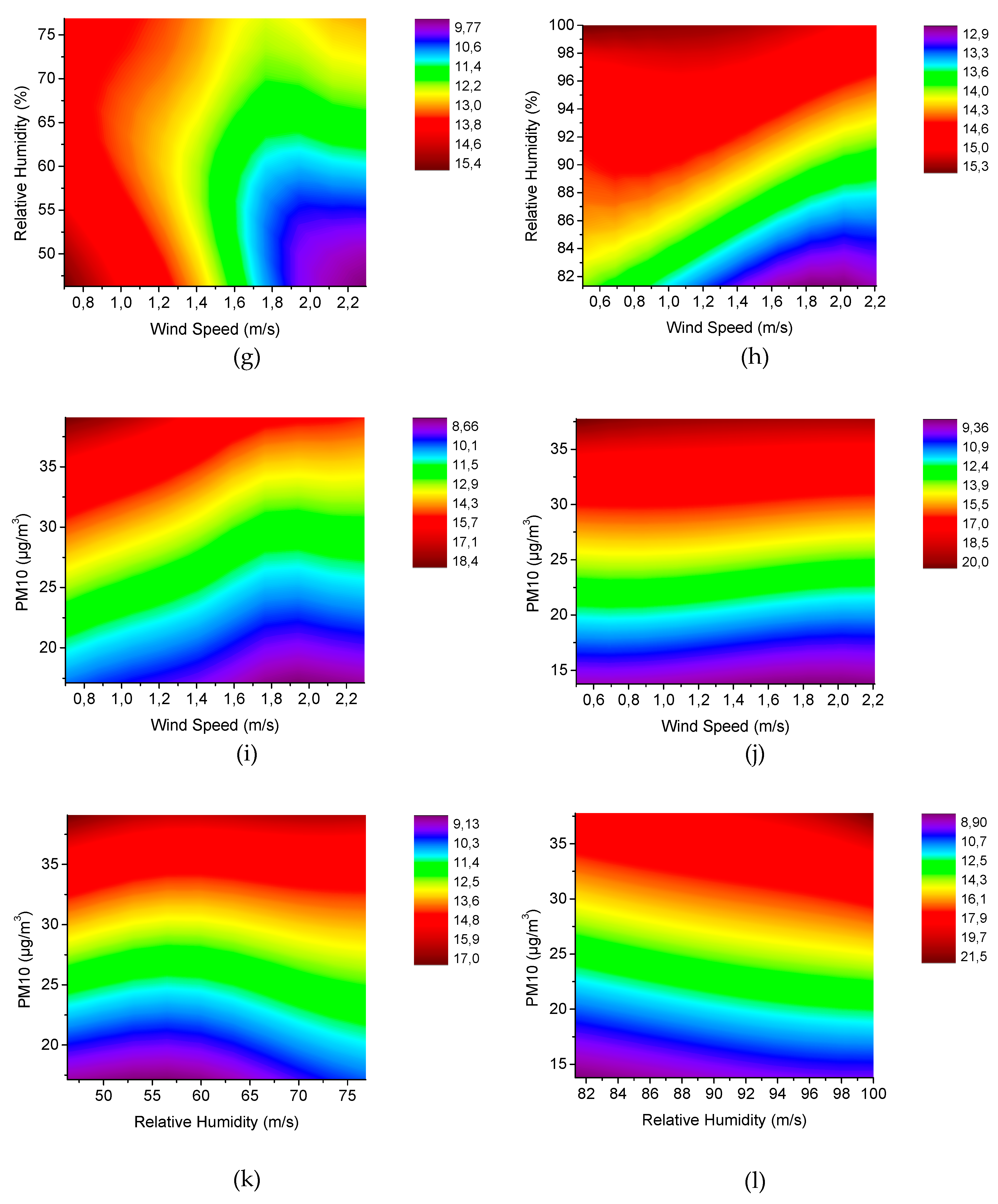
Figure 17 presents the combined effects of temperature (T), wind speed (WS), relative humidity (RH) and PM10 concentrations (PM10) on PM2.5 concentrations, for two different regimes (RH < 79.1% and for RH ≥ 79.1%), at SIUCTR (Istanbul). These results were obtained from the determined model based on the 2015–2016 period because this period allowed for evaluating the effect of all the variables mentioned above for both regimes. These explanatory variables are also commonly found as prominent in PM2.5 behaviors by different authors [7,38,42,43,59,60,61,62,63].
These results showed that, for RH < 79.1%, PM2.5 concentrations tended to: (i) decrease with T; (ii) decrease with WS; (iii) slightly decrease with RH, except when T > 23.0 °C and WS > 1.9 m/s; (iv) strongly increase with PM10. For RH ≥ 79.1%, PM2.5 concentrations tended to (i) decrease with T; (ii) decrease with WS, except when T < 10.7 °C; (iii) increase with RH; and (iv) strongly increase with PM10.
The behaviors observed for the combined effects of T–PM10, WS–PM10 and RH–PM10 were similar between the two regimes, with the relation between PM10 presence and PM2.5 concentrations prevailing over the meteorological variables. This behavior was expected, considering that some PM sources are common for both pollutants. The combined effect of T–PM10 showed that the PM10 influence on PM2.5 concentrations was higher during lower T. In the case of T–WS, PM2.5 concentrations presented to be more influenced by T when RH ≥ 79.1%. For T-RH, RH presented the opposite behavior between the two regimes for lower T. For RH-WS, RH presented the opposite behavior between the two regimes for lower WS and PM2.5 concentrations were more influenced by RH when RH ≥ 79.1%. These behaviors also indicate that the effect of WS was lower for high RH, possibly because RH is linked to the agglomeration of the particles, which weakens the influence of WS [38,62].
The observed decreases of PM2.5 concentrations with T might be associated with combustion for central heating and stronger thermal inversion conditions during cold seasons, and with the evaporation of ammonium nitrate (an important constituent of PM2.5) during warm seasons [7,35,36]. Decreases of PM2.5 with WS can be linked to the dispersion of PM away from the sources [7,43,60,62,63]. Increases of PM2.5 with WS observed during low T, for RH ≥ 79.1%, can be attributed to higher levels of dust resuspension [48]. Higher PM2.5 concentrations were observed in the second regime (HR ≥ 79.1%) when compared to the first regime (HR < 79.1%). Humidity is linked to the higher formation of sulphate and nitrate (constituents of PM2.5) and reduces the amount of solar radiation in the atmosphere, promoting temperature inversion episodes, which might be the causes to that behavior [7,57,63]. Decreases of PM2.5 with RH, like the one observed for RH < 79.1% during lower WS and T, can be associated with the stronger agglomeration of the particles, which makes them deposit from the air, reducing their concentration in the atmosphere [38,62]. Lower WS and T are associated with a higher stability of particles in the atmosphere, which enhances this behavior.
4. Conclusions
PM2.5 concentrations presented significant variations across the European sites. The highest concentrations were observed at sites strongly influenced by traffic. Compared to central and southern Europe, northern cities presented lower PM2.5 levels. In general, PM2.5 concentrations were usually higher during the winter and tended to present strong increases during rush hours, which indicates the relevance of central heating and traffic as anthropogenic PM2.5 sources. Significant spatial variations were also observed in terms of PM2.5 / PM10 ratios. These ratios were slightly higher at background sites, and the lower values were found at sites located in northern Europe (Helsinki and Stockholm), while no clear spatiality was observed for the rest of the continent. PM2.5 / PM10 ratios were usually higher during cold months and during the night.
Threshold ANN models defined with GA allowed for evaluating the combined effect of different explanatory variables on PM2.5 concentrations at SIUCTR (Istanbul). These models defined a month value of 0.92 (M < 0.92 refers to the period from January to April and August to December and M ≥ 0.92 refers to the period from May to July), RH of 79.1%, and T of 11.2 °C as the variables that could set different regimes for PM2.5 concentrations. The results showed that PM2.5 concentrations decreased with T and strongly increased with PM10 concentrations on both regimes. WS presented a negative effect on PM2.5 concentrations, except for RH ≥ 79.1% when T < 10.7 °C. The effect of WS was shown to be lower for high RH. PM2.5 decreased with RH for RH < 79.1%, except when T > 23.0 °C and WS > 1.9 m/s. For RH ≥ 79.1%, PM2.5 increased with RH. The specific objectives proposed for this study were achieved, which allowed for developing important information about the temporal and spatial trends and behaviors of PM2.5 concentrations observed in different European locations in recent years.
Author Contributions
Conceptualization, J.C.M.P.; methodology, J.A. and J.C.M.P.; software, J.C.M.P.; investigation, J.A.; data curation, J.A. and J.C.M.P.; writing—original draft preparation, J.A..; writing—review and editing, J.C.M.P.; supervision, J.C.M.P.
Funding
This research received no external funding.
Acknowledgments
This work was financially supported by the Project UID/EQU/00511/2019–Laboratory for Process Engineering, Environment, Biotechnology and Energy (LEPABE) funded by national funds through FCT/MCTES (PIDDAC). J.C.M.P. acknowledges the Foundation for Science and Technology (FCT) Investigator 2015 Programme (IF/01341/2015). The authors appreciate the availability of data from the following institutions: European Environment Agency, Ministry Of Environment And Energy Of Greece, Helsinki Region Environmental Services Authority, Republic Of Turkey Ministry Of Environment And Urbanization, Portuguese Environment Agency, London Air Quality Network-King’s College London, Ayuntamiento De Madrid, Airparif, Swedish Meteorological And Hydrological Institute, and the Provincial Government Of Vienna.
Conflicts of Interest
The authors declare no conflict of interest.
References
- WHO. 9 Out of 10 People Worldwide Breathe Polluted Air, But More Countries Are Taking Action. Available online: https://www.who.int/airpollution/en/ (accessed on 19 March 2019).
- Eeftens, M.; Tsai, M.Y.; Ampe, C.; Anwander, B.; Beelen, R.; Bellander, T.; Cesaroni, G.; Cirach, M.; Cyrys, J.; de Hoogh, K.; et al. Spatial variation of PM2.5, PM10, PM2.5 absorbance and PMcoarse concentrations between and within 20 European study areas and the relationship with NO2- Results of the ESCAPE project. Atmos. Environ. 2012, 62, 303–317. [Google Scholar] [CrossRef]
- Tallon, L.A.; Manjourides, J.; Pun, V.C.; Salhi, C.; Suh, H. Cognitive impacts of ambient air pollution in the National Social Health and Aging Project (NSHAP) cohort. Environ. Int. 2017, 104, 102–109. [Google Scholar] [CrossRef] [PubMed]
- Ailshire, J.A.; Clarke, P. Fine particulate matter air pollution and cognitive function among U.S. older adults. J. Gerontol.-Ser. B Psychol. Sci. Soc. Sci. 2015, 70, 322–328. [Google Scholar] [CrossRef] [PubMed]
- Xu, G.; Jiao, L.; Zhang, B.; Zhao, S.; Yuan, M.; Gu, Y.; Liu, J.; Tang, X. Spatial and temporal variability of the PM2.5/PM10 ratio in Wuhan, Central China. Aerosol Air Qual. Res. 2017, 17, 741–751. [Google Scholar] [CrossRef]
- Munir, S. Analysing temporal trends in the ratios of PM2.5/PM10 in the UK. Aerosol Air Qual. Res. 2017, 17, 34–48. [Google Scholar] [CrossRef]
- Megaritis, A.G.; Fountoukis, C.; Charalampidis, P.E.; Denier Van Der Gon, H.A.C.; Pilinis, C.; Pandis, S.N. Linking climate and air quality over Europe: Effects of meteorology on PM2.5 concentrations. Atmos. Chem. Phys. 2014, 14, 10283–10298. [Google Scholar] [CrossRef]
- Daly, A.; Zannetti, P. Air Pollution Modeling-An Overview. Ambient Air Pollut. 2007, I, 15–28. [Google Scholar]
- Pisoni, E.; Guerreiro, C.; Lopez-Aparicio, S.; Guevara, M.; Tarrason, L.; Janssen, S.; Thunis, P.; Pfäfflin, F.; Piersanti, A.; Briganti, G.; et al. Supporting the improvement of air quality management practices: The “FAIRMODE pilot” activity. J. Environ. Manage. 2019, 245, 122–130. [Google Scholar] [CrossRef]
- Font, A.; Guiseppin, L.; Blangiardo, M.; Ghersi, V.; Fuller, G.W. A tale of two cities: is air pollution improving in Paris and London? Environ. Pollut. 2019, 249, 1–12. [Google Scholar] [CrossRef]
- EEA. Air quality in Europe—2018 report. Available online: https://www.eea.europa.eu/publications/air-quality-in-europe-2018 (accessed on 31 July 2019).
- Karanasiou, A.; Querol, X.; Alastuey, A.; Perez, N.; Pey, J.; Perrino, C.; Berti, G.; Gandini, M.; Poluzzi, V.; Ferrari, S.; et al. Particulate matter and gaseous pollutants in the Mediterranean Basin: Results from the MED-PARTICLES project. Sci. Total Environ. 2014, 488–489, 297–315. [Google Scholar] [CrossRef]
- Zhang, G.; Patuwo, B.E.; Hu, M.Y. Forecasting with artificial neural networks: The state of the art. Int. J. Forecast. 1998, 14, 35–62. [Google Scholar] [CrossRef]
- Mahajan, R.; Kaur, G. Neural Networks using Genetic Algorithms. Int. J. Comput. Appl. 2013, 77, 6–11. [Google Scholar] [CrossRef]
- Mlakar, P.; Zlata, M. Artificial Neural Networks - a Useful Tool in Air Pollution and Meteorological Modelling. Adv. Air Pollut. 2012. [Google Scholar]
- Maciąg, P.S.; Kasabov, N.; Kryszkiewicz, M.; Bembenik, R. Air pollution prediction with clustering-based ensemble of evolving spiking neural networks and a case study on London area. Environ. Model. Softw. 2019, 118, 262–280. [Google Scholar] [CrossRef]
- Pires, J.C.M.; Gonçalves, B.; Azevedo, F.G.; Carneiro, A.P.; Rego, N.; Assembleia, A.J.B.; Lima, J.F.B.; Silva, P.A.; Alves, C.; Martins, F.G. Optimization of artificial neural network models through genetic algorithms for surface ozone concentration forecasting. Environ. Sci. Pollut. Res. 2012, 19, 3228–3234. [Google Scholar] [CrossRef]
- Vanneschi, L.; Castelli, M. Multilayer Perceptrons. In Encyclopedia of Bioinformatics and Computational Biology; Elsevier: Amsterdam, The Netherlands, 2018. [Google Scholar]
- Huang, X.H.H.; Bian, Q.; Ng, W.M.; Louie, P.K.K.; Yu, J.Z. Characterization of PM2.5 major components and source investigation in suburban Hong Kong: A one year monitoring study. Aerosol Air Qual. Res. 2014, 14, 237–250. [Google Scholar] [CrossRef]
- Hao, Y.; Deng, S.; Yang, Y.; Song, W.; Tong, H.; Qiu, Z. Chemical composition of particulate matter from traffic emissions in a road tunnel in Xi’an, China. Aerosol Air Qual. Res. 2019, 19, 234–246. [Google Scholar] [CrossRef]
- Amaral, S.S.; de Carvalho, J.A.; Costa, M.A.M.; Pinheiro, C. An overview of particulate matter measurement instruments. Atmosphere 2015, 6, 1327–1345. [Google Scholar] [CrossRef]
- Pires, J.C.M.; Sousa, S.I.V.; Pereira, M.C.; Alvim-Ferraz, M.C.M.; Martins, F.G. Management of air quality monitoring using principal component and cluster analysis-Part I: SO2 and PM10. Atmos. Environ. 2008, 42, 1249–1260. [Google Scholar] [CrossRef]
- Afonso, N.; Pires, J. Characterization of Surface Ozone Behavior at Different Regimes. Appl. Sci. 2017, 7, 944. [Google Scholar] [CrossRef]
- Botchkarev, A. Performance Metrics (Error Measures) in Machine Learning Regression, Forecasting and Prognostics: Properties and Typology. Interdiscip. J. Inf. Knowl. Manag. 2019, 14, 45–79. [Google Scholar]
- Willmott, C.J.; Ackleson, S.G.; Davis, R.E.; Feddema, J.J.; Klink, K.M.; Legates, D.R.; O’Donnell, J.; Rowe, C.M. Statistics for the evaluation and comparison of models. J. Geophys. Res. 1985, 90, 8995. [Google Scholar] [CrossRef]
- Dimitriou, K.; Kassomenos, P. The fine and coarse particulate matter at four major Mediterranean cities: Local and regional sources. Theor. Appl. Climatol. 2013, 114, 375–391. [Google Scholar] [CrossRef]
- Querol, X.; Alastuey, A.; Rodríguez, S.; Viana, M.M.; Artíñano, B.; Salvador, P.; Mantilla, E.; Do Santos, S.G.; Patier, R.F.; De La Rosa, J.; et al. Levels of particulate matter in rural, urban and industrial sites in Spain. Sci. Total Environ. 2004, 334–335, 359–376. [Google Scholar] [CrossRef]
- Querol, X.; Alastuey, A.; Ruiz, C.R.; Artiñano, B.; Hansson, H.C.; Harrison, R.M.; Buringh, E.; Ten Brink, H.M.; Lutz, M.; Bruckmann, P.; et al. Speciation and origin of PM10 and PM2.5 in selected European cities. Atmos. Environ. 2004, 38, 6547–6555. [Google Scholar] [CrossRef]
- Kopanakis, I.; Mammi-Galani, Ε.; Pentari, D.; Glytsos, T.; Lazaridis, M. Ambient Particulate Matter Concentration Levels and their Origin During Dust Event Episodes in the Eastern Mediterranean. Aerosol Sci. Eng. 2018, 2, 61–73. [Google Scholar] [CrossRef]
- Lamancusa, C.; Wagstrom, K. Global transport of dust emitted from different regions of the sahara. Atmos. Environ. 2019, 1–10. [Google Scholar] [CrossRef]
- Querol, X.; Pérez, N.; Reche, C.; Ealo, M.; Ripoll, A.; Tur, J.; Pandolfi, M.; Pey, J.; Salvador, P.; Moreno, T.; et al. African dust and air quality over Spain: Is it only dust that matters? Sci. Total Environ. 2019, 686, 737–752. [Google Scholar] [CrossRef]
- Air Quality Expert Group. Fine Particulate Matter in the United Kingdom. 2012. Available online: https://uk-air.defra.gov.uk/assets/documents/reports/cat11/1212141150_AQEG_Fine_Particulate_Matter_in_the_UK.pdf (accessed on 31 July 2019).
- Marcazzan, G.M.; Vaccaro, S.; Valli, G.; Vecchi, R. Characterisation of PM10 and PM2.5 particulate matter in the ambient air of Milan (Italy). Atmos. Environ. 2001, 35, 4639–4650. [Google Scholar] [CrossRef]
- Trinh, T.T.; Trinh, T.T.; Le, T.T.; Nguyen, T.D.H.; Tu, B.M. Temperature inversion and air pollution relationship, and its effects on human health in Hanoi City, Vietnam. Environ. Geochem. Health 2019, 41, 929–937. [Google Scholar] [CrossRef]
- Wang, Z.-b.; Fang, C.-l. Spatial-temporal characteristics and determinants of PM2.5 in the Bohai Rim Urban Agglomeration. Chemosphere 2016, 148, 148–162. [Google Scholar] [CrossRef] [PubMed]
- Yuan, S.; Xu, W.; Liu, Z. A Study on the Model for Heating Influence on PM2.5 Emission in Beijing China. Procedia Eng. 2015, 121, 612–620. [Google Scholar] [CrossRef]
- Stadt Wien Municipal Department for Environmental Protection Vienna. Vienna environmental report 2006|2007. Available online: https://www.wien.gv.at/english/environment/protection/reports/pdf/complete-06.pdf (accessed on 31 July 2019).
- Chen, T.; He, J.; Lu, X.; She, J.; Guan, Z. Spatial and temporal variations of PM2.5 and its relation to meteorological factors in the urban area of Nanjing, China. Int. J. Environ. Res. Public Health 2016, 13, 921. [Google Scholar] [CrossRef] [PubMed]
- Li, R.; Li, Z.; Gao, W.; Ding, W.; Xu, Q.; Song, X. Diurnal, seasonal, and spatial variation of PM2.5 in Beijing. Sci. Bull. 2015, 60, 387–395. [Google Scholar] [CrossRef]
- Liu, Z.; Hu, B.; Wang, L.; Wu, F.; Gao, W.; Wang, Y. Seasonal and diurnal variation in particulate matter (PM10 and PM2.5) at an urban site of beijing: Analyses from a 9-year study. Environ. Sci. Pollut. Res. 2015, 22, 627–642. [Google Scholar] [CrossRef] [PubMed]
- Tiwary, A.; Colls, J. Air Pollution: Measurement, Modelling and Mitigation; CRC Press: Boca Raton, FL, USA, 2013; Volume 47. [Google Scholar]
- Yang, Q.; Yuan, Q.; Li, T.; Shen, H.; Zhang, L. The relationships between PM2.5 and meteorological factors in China: Seasonal and regional variations. Int. J. Environ. Res. Public Health 2017, 14, 1510. [Google Scholar] [CrossRef]
- Barmpadimos, I.; Keller, J.; Oderbolz, D.; Hueglin, C.; Prévôt, A.S.H. One decade of parallel fine (PM2.5) and coarse (PM10-PM2.5) particulate matter measurements in Europe: Trends and variability. Atmos. Chem. Phys. 2012, 12, 3189–3203. [Google Scholar] [CrossRef]
- Guenther, A. A global model of natural volatile organic compound emissions. J. Geophys. Res. 1995. [Google Scholar] [CrossRef]
- Sartelet, K.N.; Couvidat, F.; Seigneur, C.; Roustan, Y. Impact of biogenic emissions on air quality over Europe and North America. Atmos. Environ. 2012, 53, 131–141. [Google Scholar] [CrossRef] [Green Version]
- Pun, B.K.; Wu, S.Y.; Seigneur, C. Contribution of biogenic emissions to the formation of ozone and particulate matter in the Eastern United States. Environ. Sci. Technol. 2002, 36, 3586–3596. [Google Scholar] [CrossRef]
- Vassilakos, C.; Saraga, D.; Maggos, T.; Michopoulos, J.; Pateraki, S.; Helmis, C.G. Temporal variations of PM2.5 in the ambient air of a suburban site in Athens, Greece. Sci. Total Environ. 2005, 349, 223–231. [Google Scholar] [CrossRef] [PubMed]
- Kassomenos, P.A.; Vardoulakis, S.; Chaloulakou, A.; Paschalidou, A.K.; Grivas, G.; Borge, R.; Lumbreras, J. Study of PM10 and PM2.5 levels in three European cities: Analysis of intra and inter urban variations. Atmos. Environ. 2014, 87, 153–163. [Google Scholar] [CrossRef]
- Duchi, R.; Cristofanelli, P.; Landi, T.C.; Arduini, J.; Bonafe’, U.; Bourcier, L.; Busetto, M.; Calzolari, F.; Marinoni, A.; Putero, D.; et al. Long-term (2002–2012) investigation of Saharan dust transport events at Mt. Cimone GAW global station, Italy (2165 m a.s.l.). Elem. Sci. Anthr. 2016, 4. [Google Scholar] [CrossRef]
- Matassoni, L.; Pratesi, G.; Centioli, D.; Cadoni, F.; Malesani, P.; Caricchia, A.M.; Di Bucchianico, A.D.M. Saharan dust episodes in Italy: Influence on PM10 daily limit value (DLV) exceedances and the related synoptic. J. Environ. Monit. 2009, 11, 1586–1594. [Google Scholar] [CrossRef] [PubMed]
- Tiwari, S.; Srivastava, A.K.; Bisht, D.S.; Parmita, P.; Srivastava, M.K.; Attri, S.D. Diurnal and seasonal variations of black carbon and PM2.5 over New Delhi, India: Influence of meteorology. Atmos. Res. 2013, 125–126, 50–62. [Google Scholar] [CrossRef]
- Zhao, X.; Zhang, X.; Xu, X.; Xu, J.; Meng, W.; Pu, W. Seasonal and diurnal variations of ambient PM2.5 concentration in urban and rural environments in Beijing. Atmos. Environ. 2009, 43, 2893–2900. [Google Scholar] [CrossRef]
- Finnish Meteorological Institute Temperature inversions. Available online: https://en.ilmatieteenlaitos.fi/temperature-inversions (accessed on 25 June 2019).
- Liu, Z.; Hu, B.; Ji, D.; Wang, Y.; Wang, M.; Wang, Y. Diurnal and seasonal variation of the PM2.5 apparent particle density in Beijing, China. Atmos. Environ. 2015, 120, 328–338. [Google Scholar] [CrossRef]
- Srimuruganandam, B.; Shiva Nagendra, S.M. Characteristics of particulate matter and heterogeneous traffic in the urban area of India. Atmos. Environ. 2011, 45, 3091–3102. [Google Scholar] [CrossRef]
- Ferm, M.; Sjöberg, K. Concentrations and emission factors for PM2.5 and PM10 from road traffic in Sweden. Atmos. Environ. 2015, 119, 211–219. [Google Scholar] [CrossRef]
- Pateraki, S.; Asimakopoulos, D.N.; Maggos, T.; Flocas, H.A.; Vasilakos, C. The role of wind, temperature and relative humidity on PM fractions in a suburban mediterranean region. Fresenius Environ. Bull. 2010, 19, 2013–2018. [Google Scholar]
- Sorek-Hamer, M.; Broday, D.M.; Chatfield, R.; Esswein, R.; Stafoggia, M.; Lepeule, J.; Lyapustin, A.; Kloog, I. Monthly analysis of PM ratio characteristics and its relation to AOD. J. Air Waste Manag. Assoc. 2017, 67, 27–38. [Google Scholar] [CrossRef] [PubMed]
- Chen, Z.; Xie, X.; Cai, J.; Chen, D.; Gao, B.; He, B.; Cheng, N.; Xu, B. Understanding meteorological influences on PM2.5 concentrations across China: A temporal and spatial perspective. Atmos. Chem. Phys. 2018, 18, 5343–5358. [Google Scholar] [CrossRef]
- Munir, S.; Habeebullah, T.M.; Mohammed, A.M.F.; Morsy, E.A.; Rehan, M.; Ali, K. Analysing PM2.5 and its association with PM10 and meteorology in the arid climate of Makkah, Saudi Arabia. Aerosol Air Qual. Res. 2017, 17, 453–464. [Google Scholar] [CrossRef]
- Tai, A.P.K.; Mickley, L.J.; Jacob, D.J. Correlations between fine particulate matter (PM2.5) and meteorological variables in the United States: Implications for the sensitivity of PM2.5 to climate change. Atmos. Environ. 2010, 44, 3976–3984. [Google Scholar] [CrossRef]
- Wang, J.; Ogawa, S. Effects of meteorological conditions on PM2.5 concentrations in Nagasaki, Japan. Int. J. Environ. Res. Public Health 2015, 12, 9089–9101. [Google Scholar] [CrossRef]
- Yadav, R.; Sahu, L.K.; Beig, G.; Tripathi, N.; Maji, S.; Jaaffrey, S.N.A. The role of local meteorology on ambient particulate and gaseous species at an urban site of western India. Urban Clim. 2019, 28, 1–10. [Google Scholar] [CrossRef]
Figure 1.
Geographical distribution of selected European cities (study area).

Figure 2.
Artificial Neural Network (ANN) scheme [13].
Figure 2.
Artificial Neural Network (ANN) scheme [13].

Figure 3.
Distribution of hourly PM2.5 concentrations for the study period.

Figure 4.
Annual average profiles of PM2.5 concentrations (urban traffic sites).

Figure 5.
Annual profiles of PM2.5 concentrations (urban background sites).

Figure 6.
Annual profiles of PM2.5 concentrations (suburban background, urban centre, rural background, roadside and suburban traffic sites).
Figure 6.
Annual profiles of PM2.5 concentrations (suburban background, urban centre, rural background, roadside and suburban traffic sites).

Figure 7.
Daily profiles of PM2.5 concentrations (urban traffic sites).

Figure 8.
Daily profiles of PM2.5 concentrations (urban background sites).

Figure 9.
Daily profiles of PM2.5 concentrations (suburban background, urban centre, rural background, roadside and suburban traffic sites).
Figure 9.
Daily profiles of PM2.5 concentrations (suburban background, urban centre, rural background, roadside and suburban traffic sites).

Figure 10.
Distribution of hourly PM2.5/PM10 ratio values for the study period.

Figure 11.
Annual profiles of the PM2.5/PM10 ratio (urban traffic sites).

Figure 12.
Annual profiles of the PM2.5/PM10 ratio (urban background sites).

Figure 13.
Annual profiles of the PM2.5/PM10 ratio (suburban background, urban centre, rural background, roadside, and suburban traffic sites).
Figure 13.
Annual profiles of the PM2.5/PM10 ratio (suburban background, urban centre, rural background, roadside, and suburban traffic sites).

Figure 14.
Daily profiles of the PM2.5/PM10 ratio (urban traffic sites).

Figure 15.
Daily profiles of the PM2.5/PM10 ratio (urban background sites).

Figure 16.
Daily profiles of the PM2.5/PM10 ratio (suburban background, urban centre, rural background, roadside, and suburban traffic sites).
Figure 16.
Daily profiles of the PM2.5/PM10 ratio (suburban background, urban centre, rural background, roadside, and suburban traffic sites).

Figure 17.
Combined effect of temperature (°C), wind speed (m/s), relative humidity (RH, %) and PM10 concentrations (µg/m3) on PM2.5 concentrations (µg/m3) for RH < 79.1% (a,c,e,g,i,k) and RH ≥ 79.1% (b,d,f,h,j,l).
Figure 17.
Combined effect of temperature (°C), wind speed (m/s), relative humidity (RH, %) and PM10 concentrations (µg/m3) on PM2.5 concentrations (µg/m3) for RH < 79.1% (a,c,e,g,i,k) and RH ≥ 79.1% (b,d,f,h,j,l).


Table 1.
Data sources for each selected city.
| Country | City | Source |
|---|---|---|
| Netherlands | Amsterdam | European Environment Agency (EEA) |
| Greece | Athens | Ministry of Environment and Energy of Greece |
| Finland | Helsinki | Helsinki Region Environmental Services Authority |
| Turkey | Istanbul | Republic of Turkey Ministry of Environment and Urbanization |
| Portugal | Lisbon | Portuguese Environment Agency (APA) |
| England | London | London Air Quality Network–King’s College London |
| Spain | Madrid | Ayuntamiento de Madrid |
| Norway | Oslo | European Environment Agency (EEA) |
| France | Paris | Airparif |
| Czech Republic | Prague | European Environment Agency (EEA) |
| Sweden | Stockholm | Swedish Meteorological and Hydrological Institute |
| Austria | Vienna | Provincial Government of Vienna |
Table 2.
Characterization of the selected stations (identification, type, geographical location, and sampling period).
Table 2.
Characterization of the selected stations (identification, type, geographical location, and sampling period).
| Station ID | City | Station Name | Station Type | Latitude | Longitude | Altitude (m) | Sampling Period |
|---|---|---|---|---|---|---|---|
| VDUTNL | Amsterdam | Van Diemenstraat | Urban Traffic | 52.390003 | 4.888058 | 4 | 2013–2017 |
| PEUTGR | Athens | Peiraias | 37.943287 | 23.647511 | 20 | 2016–2017 | |
| MNUTFI | Helsinki | Mannerheimintie | 60.16964 | 24.93924 | 5 | 2013–2017 | |
| EAUTES | Madrid | Escuelas Aguirre | 40.421667 | −3.682222 | 672 | 2013–2017 | |
| SMUTCZ | Prague | Smichov | 50.073135 | 14.398141 | 216 | 2013–2017 | |
| HGUTSE | Stockholm | Hornsgatan 108 Gata | 59.317299 | 18.048994 | 24 | 2013–2017 | |
| TBUTAT | Vienna | Taborstraße | 48.205000 | 16.309750 | 236 | 2013–2017 | |
| WGUBNL | Amsterdam | Wagenschotpad | Urban Background | 52.450001 | 4.816667 | 1 | 2013–2017 |
| KAUBFI | Helsinki | Kallio | 60.187390 | 24.950600 | 21 | 2013–2017 | |
| LAUBPT | Lisbon | Laranjeiro | 38.663611 | −9.157778 | 63 | 2013–2017 | |
| CBUBGB | London | Camden-Bloomsbury | 51.522290 | −0.125889 | 20 | 2013–2017 | |
| MAUBES | Madrid | Méndez Álvaro | 40.420000 | −3.749167 | 645 | 2013–2017 | |
| SOUBNO | Oslo | Sofienbergparken | 59.922950 | 10.765730 | 24 | 2013–2017 | |
| GNUBFR | Paris | Gennevilliers | 48.929692 | 2.294719 | 28 | 2013–2017 | |
| TKUBSE | Stockholm | Torkel Knutssongatan | 59.316940 | 18.057501 | 58 | 2013–2017 | |
| STUBAT | Vienna | Stadlau | 48.226361 | 16.458345 | 159 | 2013–2017 | |
| LYSBGR | Athens | Lykrovisi | Suburban Background | 38.065200 | 23.787289 | 234 | 2016–2017 |
| LISBCZ | Prague | Libus | 50.007305 | 14.445933 | 301 | 2013–2017 | |
| SIUCTR | Istanbul | Silivri | Urban Centre | 41.073056 | 28.255278 | 32 | 2013–2018 |
| CHRBPT | Lisbon | Chamusca | Rural Background | 39.352500 | −8.466111 | 143 | 2013–2017 |
| LHRSGB | London | Lewisham - New Cross | Roadside | 51.474954 | −0.039641 | 25 | 2013–2017 |
| ARRSFR | Paris | Autoroute A1 - Saint-Denis | 48.925265 | 2.356667 | 35 | 2013–2017 | |
| HJSTNO | Oslo | Hjortnes | Suburban Traffic | 59.911320 | 10.704070 | 8 | 2013–2017 |
Table 3.
Characterization of the obtained models (selected explanatory variables, threshold variable and value, activation function (AF), and the number of hidden neurons (HN)).
Table 3.
Characterization of the obtained models (selected explanatory variables, threshold variable and value, activation function (AF), and the number of hidden neurons (HN)).
| Period | Model | AF | HN |
|---|---|---|---|
| 2013–2014 | tansig tansig | 8 8 | |
| 2015–2016 | radbas radbas | 8 8 | |
| 2017–2018 | tansig tansig | 8 7 |
Note: M = month of measurement; H = hour of measurement; T = temperature; WD = wind direction; WS = wind speed; RH = relative humidity; AP = air pressure; PM10 = concentration of PM10.
© 2019 by the authors. Licensee MDPI, Basel, Switzerland. This article is an open access article distributed under the terms and conditions of the Creative Commons Attribution (CC BY) license (http://creativecommons.org/licenses/by/4.0/).
Share and Cite
MDPI and ACS Style
Adães, J.; Pires, J.C.M. Analysis and Modelling of PM2.5 Temporal and Spatial Behaviors in European Cities. Sustainability 2019, 11, 6019. https://0-doi-org.brum.beds.ac.uk/10.3390/su11216019
AMA Style
Adães J, Pires JCM. Analysis and Modelling of PM2.5 Temporal and Spatial Behaviors in European Cities. Sustainability. 2019; 11(21):6019. https://0-doi-org.brum.beds.ac.uk/10.3390/su11216019
Chicago/Turabian StyleAdães, José, and José C. M. Pires. 2019. "Analysis and Modelling of PM2.5 Temporal and Spatial Behaviors in European Cities" Sustainability 11, no. 21: 6019. https://0-doi-org.brum.beds.ac.uk/10.3390/su11216019
Note that from the first issue of 2016, this journal uses article numbers instead of page numbers. See further details here.