Considering JIT in Assigning Task for Return Vehicle in Green Supply Chain

Abstract

The purpose of this study was to achieve supply chain sustainability by considering Just in Time (JIT) in return vehicle usage. In response to a general increase in modern environmental awareness, consumer and government attention towards product and service compliance with environmental protection standards has increased. Consequently, manufacturers and stakeholders are pressured to use eco-friendly supply chains. In this paper, we analyzed the JIT model, a transportation network that ensure agile responses and delivery of goods in a supply chain, which reduces inventory costs. We then compared two return vehicle transportation scenarios. In the first, goods were transported from the central warehouse to the distribution base, and the return vehicle delivered recyclable packaging materials back to the central distribution warehouse. In the second scenario, goods were transported from the manufacturer to the distribution center (warehouse) more frequently, leading to reduced inventory. We then utilized the aforementioned JIT system with ILOG CPLEX12.4 to ascertain which scenario would produce the lowest carbon emissions for the lowest total cost.

1. Introduction

People’s growing concern about whether or not the commodities they purchase are environmentally friendly and energy saving has gradually exerted an influence on consumer purchasing behavior, leading to a boom in green supply chain developments, which covers green purchases, manufacturing, green consumption, recycling, green logistics, etc. [1,2]. Porter and Van der Linde [3] provided an analysis of various theories about the supply chain, arguing that the greening of companies will be an integrative process that will increase their competitive advantage. Based on a compilation of state-of-the-art green supply chain literature, Srivastava [4] proposed that its main focuses are green operations, green design, reverse logistics, network design, green manufacture, re-manufacture, and waste management. Wang et al. [5] adopted the company site selection issue as the strategic planning theme, using the multi-objective optimization model to solve the problem of balancing cost and protecting the environment. They concluded that the higher the supply chain network capacity, the lower the carbon emissions and cost. Green et al. [6] explored the impact of the implementation of the green supply chain on the performance of the manufacturing sector in the United States. Adoption of the green supply chain has had a significantly positive impact on environmental, operational, and organizational performance.

Furthermore, the manufacturers and stakeholder have raised their efforts towards implemented carbon management practices due to pressure on carbon disclosure information [7]. According to Herold [8], companies not only increased the implemented internal and external carbon disclosure management practices but have also implemented internal carbon disclosure measurement. Tognetti [9] explored the impact of carbon emissions on the entire supply chain of the automobile industry in Germany and designed a green supply chain optimization mathematical model to find solutions. Provided that the costs do not increase, the carbon emissions can be reduced by 30%. Through [10] investigation of the relationship between carbon prices and fuel prices, these researchers found that when priced at US$30–40 per ton, carbon emission reduction is significant, while a 30% reduction in fuel cost can be balanced by increasing the carbon price to US$30 per ton. Companies that have implemented the sustainable green concept have been shown to have a better operational and organizational performance [8]. Therefore, this trend is not only environmentally friendly but will also enhance enterprise competitiveness through supply chain network integration [3].

In addition, it is well known that high-tech products (computers, mobile phones, etc.) which have a high heavy metal content, without proper disposal, will result in serious environmental damage [11,12]. Thus, reverse logistics in the supply chain plays a protective role on the environment by ensuring the recycling of such products. Through reverse transportation, these items can be reused in the supply chain, leading to a more comprehensive supply chain under forward and reverse transportation scenarios. Wei et al. [13] proposed an inventory control model of recycling and a re-manufacturing process with uncertain needs. The research was established based on a limited plan scope—the manufacturing process integration and entry into the product recycling process. Mitra [14] established a two-order inventory closed-loop supply chain system, including both certain and random factors to analyze the following questions: 1. Why are the costs of the closed-loop supply chain higher compared to the traditional supply chain? 2. Will the total costs be reduced if the high recycling rate is converted into low demand? 3. What are the relationships among expected costs, demand, and recycling? In addition, the supply chain of the mixed integral linear planning implements reverses circulation design and planning by simultaneously taking into account production, distribution, and reverse logistics activities [15]. Zikopoulos and Tagaras [16] assumed a reverse supply chain target function with a negative collection station, the parameters of which include the possibility of recycling sequence, assumptive needs, and recycling quality.

Generally, the current forms of transportation cannot yet achieve zero-pollutant emissions. The transportation industry ranks the highest in the supply chain in terms of the air pollutant volume produced each year other than by manufacturing plants under specific situations [17]. In response, a greater number of companies have chosen to hire third-party specialists to handle logistical distribution in the supply chain [18]. This has been shown not only to reduce transportation costs but also to improve service and operational efficiency [19]. It can also allow for the possibility of reverse logistics, thus achieving the concept of overall logistical continuity. Hence, the use of these specialists in distribution is now an essential part of sustainable logistics.

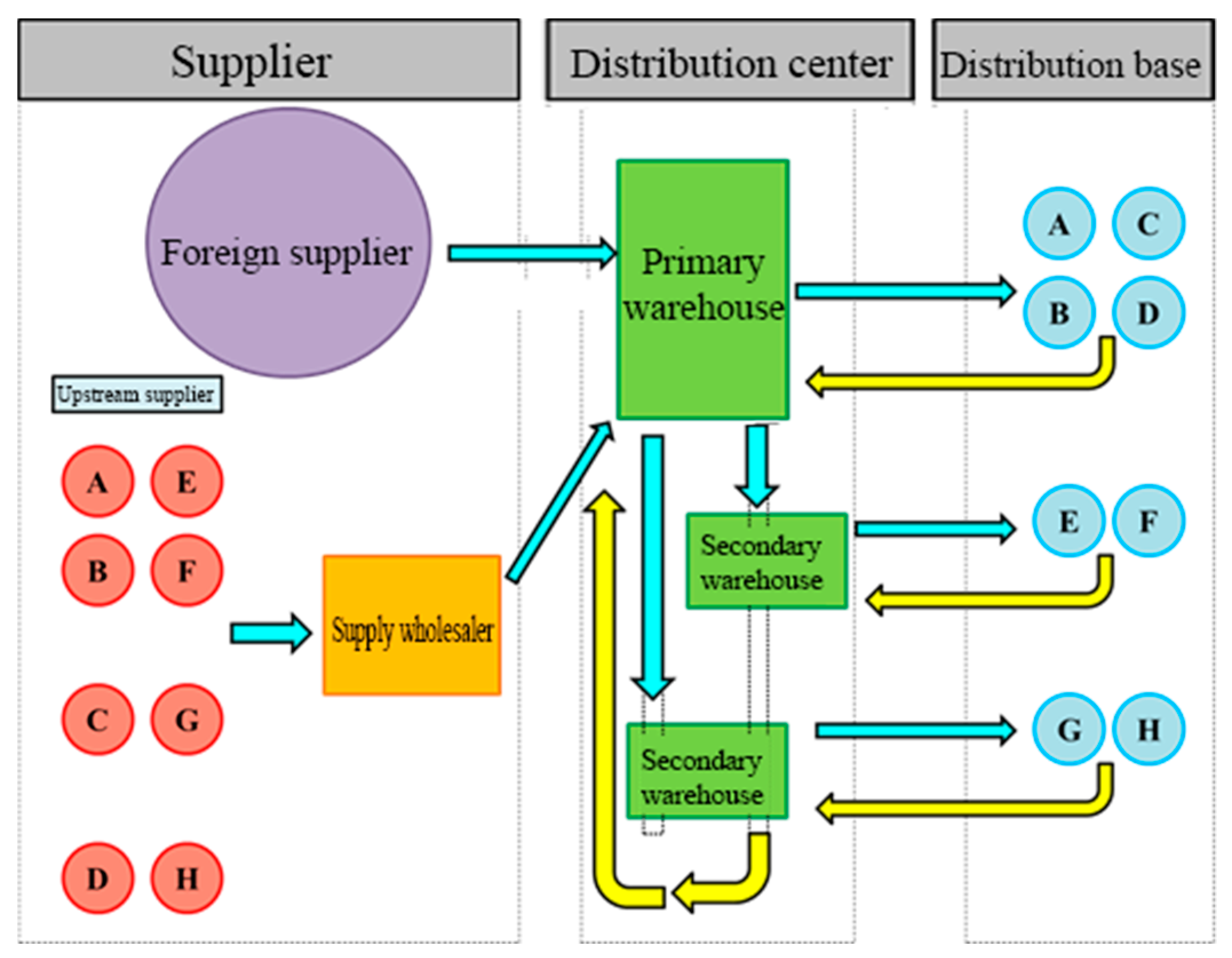
Third-party logistics utilize end-point distribution models in the supply chain to increase energy conservation [20]. For example, the supply chain for the distribution of the automobile industry’s repair parts is divided into three levels: the suppliers, the distribution center (warehouse), and the distribution bases [21]. In [21], the first group included foreign and upstream suppliers as well as supply wholesalers. The supply wholesaler is mainly responsible for stockpiling the goods of upstream suppliers. Then, based on various consumer needs, purchase orders and goods are distributed. The supply manufacturer’s major customer is the automobile parts distribution center (warehouse), which transports parts to automobile manufacturing plants. Since the automobile manufacturing plant is a separate supply chain, it will not be discussed here. Various parts are stored at the distribution center (warehouse), which are distributed by third-party logistical specialists based on the needs of the downstream distribution bases.

After the goods arrive at their destination, the specialists must determine how to plan the delivery trucks efficiently as return vehicle utilization, which remains a crucial aspect of the green supply chain. It is indeed challenging to use return vehicles for reverse logistics or for the transportation of new goods. A typical route of the supply chain logistics network is shown in Figure 1 (the yellow arrow represents the return trip). After the distribution of goods by a third-party logistics specialist, the return vehicle heads to the original warehouse. However, if no goods are loaded on the return trip, it is a waste. Hence, in order to ensure a better efficiency of the supply chain, it is important to determine how best to strengthen information circulation in the supply chain and enable the third-party logistic specialists to utilize effectively the return vehicles for goods distribution.

Therefore, in this study, we hypothesized that better utilization of returning vehicles of the distribution process in the logistics network holds significant importance [22]. How to utilize return vehicles to most efficiently load goods remains a difficult real-world NP problem, which leaves much room for testing and research. However, if new goods could be loaded at the bases at the same time as when these vehicles deliver goods there, this would maximize vehicle efficiency. In addition, goods would be safely packaged using green materials. Today’s automobile repair parts (sheet metal parts) must be well packaged to ensure that they are delivered safely and to facilitate transportation convenience. It must be noted that this type of packaging material can be recycled and reused. According to the data of the company, this type of packaging material can be directly reused three to four times. Thus, the reverse logistics of recycling and delivery of packaging materials are vital in the supply chain [23,24,25].

In addition, due to peoples’ dependence on automobiles, a driver needs to know how long it will take for his or her car to be repaired after sending it to the garage. Thus, it is essential for the automobile repair parts industry to achieve high service standards for efficiency. In fact, consumers are willing to pay the high inventory costs of stocking large quantities of parts at the garage in exchange for the convenience of a short wait time. However, since it is impossible for small warehouses to store a wide variety of automobile parts, garages stock parts that are most often used in typical repairs. Rarer parts must be ordered and sent before repairs can be done. This being said, the speed of distribution is very important at the supply chain end, since only companies that can respond promptly are able to maintain a high standard of service.

In pursuit of a faster response, many inventory management strategies have emerged, such as efficient consumer response, Just in Time (JIT), ship order production, and demand-supply [26,27]. The Just in Time (JIT) approach, which was developed to address dealer inventory issues at the end of the supply chain, has become increasingly important. The goal of these strategies in the supply chain is to quickly respond to customers’ demands. Moreover, the Just in Time (JIT) strategy has forged ahead of the others by resolving the issue of distributor stocking at the supply chain end.

In order for the end distributors to efficiently respond to customers, the first-order suppliers must stock sufficient numbers and varieties of parts to promptly cope with the needs of downstream distributors. On the other hand, the bullwhip effect (demand variance amplification principle) leads to the storage of a much higher quantity of parts on the supplier’s end. The JIT management system enables customers (distributors) to lower their inventory costs [28,29]; however, this will lead to increased inventory on the supplier’s side. The automobile repair market is a good example of this phenomenon. In order to provide higher service standards that will hopefully lead to an increase in loyal customers, the garage must be able to promptly acquire various parts for repairs. Therefore, according to the JIT model, in order to quickly supply garages with automobile repair parts, upstream suppliers must stock a large quantity.

Therefore, the main purpose of this study was to properly utilize transportation in the supply chain so that transportation can load the goods with the highest utilization during the return journey. For this reason, this study proposes two scenarios for research. The first scenario is to integrate green and sustainable ideas into the supply chain network. The transportation vehicles in the supply chain have the function of both forward and reverse logistics. The packaging materials can be recycled at each point collection when the items are delivered to the bases. The purpose of this scenario is to make the supply chain more environmentally friendly and reduce the overall carbon emissions. The second scenario is to reverse the returning vehicles from the manufacturing supplier to load the goods and then deliver them directly to the distribution center. By increasing the frequency of delivery from the manufacturer to the distribution center, the supply chain can reduce the overall inventory and improve the economic effect. Through calculation and analysis, we can decide how to achieve economic and environmental trade-offs in two situations.

In Section 2, the modeling and assumptions are defined, as well as the basic model assumptions, and definitions for symbols and parameters. Pareto’s multi-objective integer programming is then proposed to solve the formulations and object functions in two scenarios. Section 3 examines the numerical sample and compares the results to the traditional supply chain, Scenario 1 and Scenario 2 cases. Finally, Section 4 concludes the summary of research findings and contributions.

2. Modeling and Assumptions

2.1. Description of the Scenarios

Assuming a four-order supply chain, the first of this study was the manufacturing supplier (manufacturer denoted as m), the second was the supply wholesaler (supplier, denoted as s), the third was the distribution center (warehouse, denote as w), and the fourth order was the distribution base (retailer, denoted as r). Additionally, the mathematical model contained two scenarios for transportation and distribution.

● Scenario 1

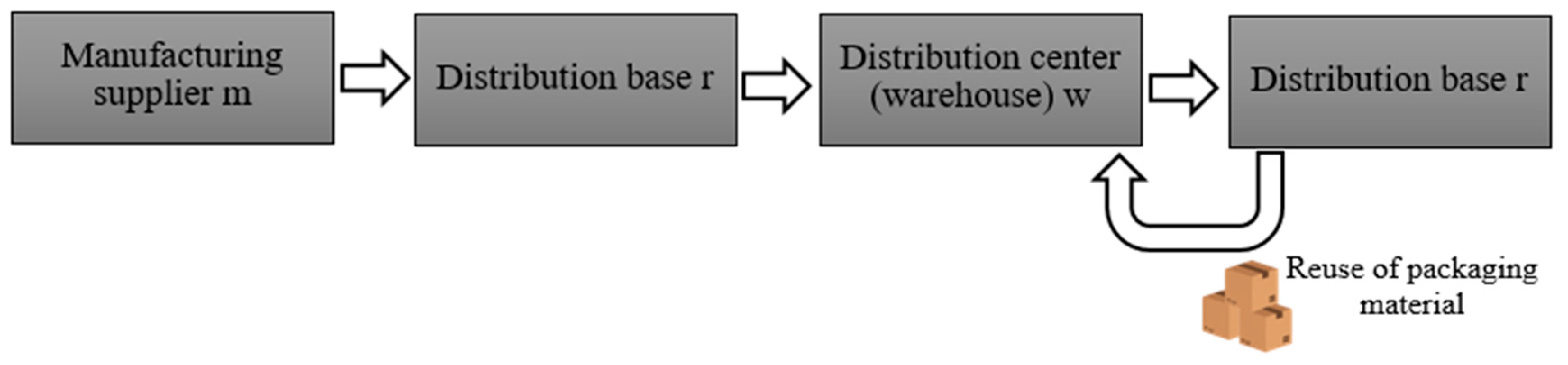
The “from the distribution center (warehouse) to the distribution base” section of the supply chain transportation model covers reverse logistical factors. After transporting goods to the distribution base, the return vehicle was then used to send the packaging material back to the distribution center (warehouse) so that it could be reused in the supply chain. At the same time, the return vehicle was utilized, which reduces carbon emissions and costs in the supply chain. The supply chain is shown in Figure 2.

● Scenario 2

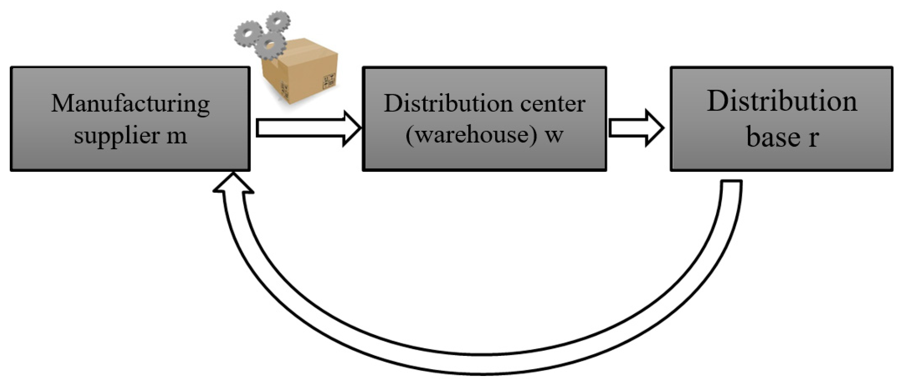
In the manufacturing supplier transportation model, vehicles transported goods from the distribution center (warehouse) to the distribution base. On the way back, they stopped at the manufacturing supplier to directly transport goods to the distribution center (warehouse), thus skipping the supply wholesaler stage and ensuring the availability of more vehicles at both ends, namely from the manufacturing supplier to the distribution center (warehouse). Reducing the lead time facilitates rapid deliveries and faster response times, thereby ensuring more stable inventory at the distribution center (warehouse) and lowering inventory levels. The overall supply chain still has four orders. Only the goods in this scenario have three orders. The supply chain is shown in Figure 3.

2.2. Basic Model Assumptions

• The demand for each period is known.
• Shortage of stock is not allowed.
• Wear and tear are not considered.
• Manufacturing suppliers are able to coordinate with those in production regarding the modes of ordering and delivery in Scenario 2.
• The ordering time is a fixed period.
• The arrival time is a fixed period.
• The inventory transport mode in situation 1 cannot be used interchangeably but must be utilized for each type of good.
• The maximum inventory-related parameters are updated every five working days.
• In Scenario 2, the maximum inventory-related coefficients LT and SSLT are fixed and are not subject to change.
• In Scenario 2, transportation vehicles going from the logistics distribution center to the distribution location sufficiently accommodate goods provided by the supply manufacturers.
• An order is placed every five working days.
• Goods arrive every ten days, a schedule equal to that of two previous orders.

2.3. Model Symbols and Definitions

Table 1. Meaning of the symbols and settings in Numerical Example.

Symbol	Meaning of the Symbols	Settings in Numerical Example
m	Manufacturer	4
s	Supplier	1
w	DC warehouse	1
r	Retailer	1
c	Packaging materials
g	Merchants
TM	Utilize the model of returning vehicle in the supply chain	1: Recycling packaging materials 2: Transport goods to upstream suppliers
n	The planning period	120
a	Number of suppliers, a = 1, …a	4
b	The types of merchandise offered by the supplier, b = 1, …b	5
S	Start ordering time of merchants

,

Table 2. Meaning of the Parameters.

Parameter	Meaning of the Parameters:
PSM	Unit cost to the supplier for purchasing products from the manufacturer
PWS	Unit cost to the DC warehouse for purchasing products from the supplier
PRW	Unit cost to the retailer for purchasing products from the DC warehouse
PWM	Unit cost to the DC warehouse for purchasing products from the manufacturer
PWC	Unit cost to the DC warehouse for purchasing packaging materials
TMS	Unit cost from the manufacturer to the supplier
TSW	Unit cost from the supplier to the DC warehouse
TWR	Unit cost from the DC warehouse to the retailer
TRM	Unit cost from the retailer to the manufacturer
TMW	Unit cost to ship from the manufacturer to the DC warehouse
FG	Unit cost to the producing merchant
FC	Unit cost of producing packaging materials
IW	Unit cost of inventory for the DC warehouse
IM	Unit cost of inventory for the manufacturer
QG	The ordering quantity of goods
MIPG	The maximum inventory in the production of goods
MADG	The maximum annual demand for goods
OCG	Order cycle time
LTG	Lead time of purchasing goods
SSDG	Safety stock with demand fluctuations for goods
SSLTG	Safety stock with lead time fluctuations of purchasing goods
OHG	On hand inventory
OOG	On-order inventory
EMS	Unit carbon emissions as a result of transportation from the manufacturer to the supplier
ESW	Unit carbon emissions as a result of transportation from the supplier to the DC warehouse
EWR	Unit carbon emissions as a result of transportation from the DC warehouse to the retailer
ERM	Unit carbon emissions as a result of transportation from the DC warehouse to the retailer
EMW	Unit carbon emissions as a result of transportation from the manufacturer to the DC warehouse
ECP	Unit carbon emissions as a result of producing packaging materials at the manufacturing plant

and

Table 3. Meaning of the Strategic-Decision Variable.

Strategic-Decision Variable	Meaning of the Strategic-Decision Variable
${\chi }_{\left(a,b\right),TM,n}$	To determine whether or not to ship product B from manufacturer A, on the nth day of the TM case.

show and defines the symbols, parameters and decision variables of our model.

2.4. The Formulation Parameters

Total cost to the supplier for purchasing products from the manufacturer:

$$PSMTC={\displaystyle \sum }_{\left(a,b\right)}{\displaystyle \sum }_{TM}\left(PS{M}_{\left(a,b\right)}\times Q{G}_{\left(a,b\right),TM}\right){\chi }_{\left(a,b\right),TM,n}$$

(1)

Total cost to the DC warehouse for purchasing products from the supplier:

$$PWSTC={\displaystyle \sum }_{\left(a,b\right)}{\displaystyle \sum }_{TM}\left(PW{S}_{\left(a,b\right)}\times Q{G}_{\left(a,b\right),TM}\right){\chi }_{\left(a,b\right),TM,n}$$

(2)

Total cost to the retailer for purchasing products from the DC warehouse:

$$PRWTC={\displaystyle \sum }_{\left(a,b\right)}{\displaystyle \sum }_{TM}\left(PR{W}_{\left(a,b\right)}\times Q{G}_{\left(a,b\right),TM}\right){\chi }_{\left(a,b\right),TM,n}$$

(3)

Total cost to the DC warehouse for purchasing products from the manufacturer:

$$PWMTC={\displaystyle \sum }_{\left(a,b\right)}{\displaystyle \sum }_{TM}\left(PW{M}_{\left(a,b\right)}\times Q{G}_{\left(a,b\right),TM}\right){\chi }_{\left(a,b\right),TM,n}$$

(4)

Total cost to the DC warehouse for purchasing packaging materials:

$$PWCTC=PWC\times (n-{{\displaystyle \sum }}_{n=1}^n{{\displaystyle \sum }}_{TM=2}{\chi }_{\left(a,b\right),TM,n})\mathrm{for}\mathrm{a}=1\dots \mathrm{A},\mathrm{b}=1\dots \mathrm{B}$$

(5)

Total cost from the manufacturer to the supplier:

$$TMSTC=TMS\times ({{\displaystyle \sum }}_{n=1}^n{{\displaystyle \sum }}_{TM=1}{\chi }_{\left(a,b\right),TM,n})\mathrm{for}\mathrm{a}=1\dots \mathrm{A},\mathrm{b}=1\dots \mathrm{B}$$

(6)

Total cost from the supplier to the DC warehouse:

$$TSWTC=TSW\times ({{\displaystyle \sum }}_{n=1}^n{{\displaystyle \sum }}_{TM=1}{\chi }_{\left(a,b\right),TM,n})\mathrm{for}\mathrm{a}=1\dots \mathrm{A},\mathrm{b}=1\dots \mathrm{B}$$

(7)

Total cost from the DC warehouse to the retailer:

$$TWRTC=TWR\times ({{\displaystyle \sum }}_{n=1}^n{{\displaystyle \sum }}_{TM=1}{\chi }_{\left(a,b\right),TM,n})\mathrm{for}\mathrm{a}=1\dots \mathrm{A},\mathrm{b}=1\dots \mathrm{B}$$

(8)

Total cost from the retailer to the manufacturer:

$$TRMTC=TWR\times ({{\displaystyle \sum }}_{n=1}^n{{\displaystyle \sum }}_{TM=1}^2{\chi }_{\left(a,b\right),TM,n})\mathrm{for}\mathrm{a}=1\dots \mathrm{A},\mathrm{b}=1\dots \mathrm{B}$$

(9)

Total cost to ship from the manufacturer to the DC warehouse:

$$TMWTC=TWR\times ({{\displaystyle \sum }}_{n=1}^n{{\displaystyle \sum }}_{TM=2}{\chi }_{\left(a,b\right),TM,n})\mathrm{for}\mathrm{a}=1\dots \mathrm{A},\mathrm{b}=1\dots \mathrm{B}$$

(10)

Total cost of inventory for the DC warehouse:

$$IWTC=IW\times ({{\displaystyle \sum }}_{n=1}^n{{\displaystyle \sum }}_{TM=1}^{2}O{H}_{\left(a,b\right),TM,n})\mathrm{for}\mathrm{a}=1\dots \mathrm{A},\mathrm{b}=1\dots \mathrm{B}$$

(11)

Total cost of inventory for the manufacturer:

$$IMTC=IW\times ({{\displaystyle \sum }}_{n=1}^n{{\displaystyle \sum }}_{TM=1}^{2}O{O}_{\left(a,b\right),TM,n})\mathrm{for}\mathrm{a}=1\dots \mathrm{A},\mathrm{b}=1\dots \mathrm{B}$$

(12)

Total cost to the producing merchant:

$$FGTC={\displaystyle \sum }_{\left(a,b\right)}{\displaystyle \sum }_{TM}\left(F{G}_{\left(a,b\right)}\times Q{G}_{\left(a,b\right),TM}\right){\chi }_{\left(a,b\right),TM,n}$$

(13)

Total cost of producing packaging materials:

$$FCTC=FC\times (n-{{\displaystyle \sum }}_{n=1}^n{{\displaystyle \sum }}_{TM=1}^2{\chi }_{\left(a,b\right),TM,n})\mathrm{for}\mathrm{a}=1\dots \mathrm{A},\mathrm{b}=1\dots \mathrm{B}$$

(14)

The ordering quantity of goods:

$$\begin{gathered} QG=MIP{G}_{\left(a,b\right),TM,n}-OH{G}_{\left(a,b\right),TM,n}-OO{G}_{\left(a,b\right),TM,n} \\ \mathrm{for}\mathrm{a}=1\dots \mathrm{A},\mathrm{b}=1\dots \mathrm{B},\mathrm{TM}=1\mathrm{or}2,\mathrm{n}=1\dots \mathrm{n} \end{gathered}$$

(15)

The maximum inventory in the production of goods:

$$\begin{gathered} MIPG=MAD{G}_{\left(a,b\right),TM,n}\left(OC{G}_{\left(a,b\right),TM,n}+LT{G}_{\left(a,b\right),TM,n}+SSD{G}_{\left(a,b\right),TM,n}+SSLT{G}_{\left(a,b\right),TM,n}\right) \\ \mathrm{for}\mathrm{a}=1\dots \mathrm{A},\mathrm{b}=1\dots \mathrm{B},\mathrm{TM}=1\mathrm{or}2,\mathrm{n}=1\dots \mathrm{n} \end{gathered}$$

(16)

Unit emissions as a result of producing packaging materials at the manufacturing plant:

$$ECPC=ECP\times (n-{{\displaystyle \sum }}_{n=1}^n{{\displaystyle \sum }}_{TM=1}^2{\chi }_{\left(a,b\right),TM,n})\mathrm{for}\mathrm{a}=1\dots \mathrm{A},\mathrm{b}=1\dots \mathrm{B}$$

(17)

Unit carbon emissions as a result of transportation from the manufacturer to the supplier:

$$EMSC=EMS\times ({{\displaystyle \sum }}_{n=1}^n{{\displaystyle \sum }}_{TM=1}{\chi }_{\left(a,b\right),TM,n})\mathrm{for}\mathrm{a}=1\dots \mathrm{A},\mathrm{b}=1\dots \mathrm{B}$$

(18)

Unit carbon emissions as a result of transportation from the supplier to the DC warehouse:

$$ESWC=ESW\times ({{\displaystyle \sum }}_{n=1}^n{{\displaystyle \sum }}_{TM=1}{\chi }_{\left(a,b\right),TM,n})\mathrm{for}\mathrm{a}=1\dots \mathrm{A},\mathrm{b}=1\dots \mathrm{B}$$

(19)

Unit carbon emissions as a result of transportation from the DC warehouse to the retailer:

$$EWRC=EWR\times ({{\displaystyle \sum }}_{n=1}^n{{\displaystyle \sum }}_{TM=1}^2{\chi }_{\left(a,b\right),TM,n})\mathrm{for}\mathrm{a}=1\dots \mathrm{A},\mathrm{b}=1\dots \mathrm{B}$$

(20)

Unit carbon emissions as a result of transportation from the DC warehouse to the retailer:

$$ERMC=ERM\times ({{\displaystyle \sum }}_{n=1}^n{{\displaystyle \sum }}_{TM=2}{\chi }_{\left(a,b\right),TM,n})\mathrm{for}\mathrm{a}=1\dots \mathrm{A},\mathrm{b}=1\dots \mathrm{B}$$

(21)

Unit carbon emissions as a result of transportation from the manufacturer to the DC warehouse:

$$EMWC=EMW\times ({{\displaystyle \sum }}_{n=1}^n{{\displaystyle \sum }}_{TM=2}{\chi }_{\left(a,b\right),TM,n})\mathrm{for}\mathrm{a}=1\dots \mathrm{A},\mathrm{b}=1\dots \mathrm{B}$$

(22)

2.5. Objective Functions and Constraints

• Objective Function 1: Minimum the total Cost:

  $$\begin{array}{cc}\hfill {\mathrm{minZ}}_1& =PSMTC+PWMTC+PRWTC+PWMTC+PWCTC+TMSTC\hfill \\ \hfill & +TSWTC+TWRTC+TRMTC+IWTC+IMTC+FGTC\hfill \\ \hfill & +FCTC\hfill \end{array}$$

  (23)
• Objective Function 2: Minimum CO₂

  $${\mathrm{minZ}}_2=ECPC+EMSC+ESWC+EWRC+ERMC+EMWC$$

  (24)
• Model Constraints:
  • Each can choose either Scenario 1 or Scenario 2 for transportation and cross usage is not allowed for 120 working days.

    $${\chi }_{\left(a,b\right),1,n}+{\chi }_{\left(a,b\right),2,n}\le 1\mathrm{for}\mathrm{a}=1,2,3,4,\mathrm{b}=1,2,\dots ,5,\mathrm{n}=\mathrm{S},\mathrm{S}+1,\dots ,\mathrm{S}+120$$

    (25)

    $${\chi }_{\left(a,b\right),TM,n+10}\ge {\chi }_{\left(a,b\right),TM,n}$$

    (26)
  • The goods arrive once every ten days.

    $${{\displaystyle \sum }}_{n=1}^{10}{\chi }_{\left(a,b\right),TM,n}=1\mathrm{for}\mathrm{a}=1,2,3,4,\mathrm{b}=1,2,\dots ,5,\mathrm{TM}=1,2$$

    (27)

    $${{\displaystyle \sum }}_{n=11}^{20}{\chi }_{\left(a,b\right),TM,n}=1\mathrm{for}\mathrm{a}=1,2,3,4,\mathrm{b}=1,2,\dots ,5,\mathrm{TM}=1,2$$

    (28)

    $${{\displaystyle \sum }}_{n=21}^{30}{\chi }_{\left(a,b\right),TM,n}=1\mathrm{for}\mathrm{a}=1,2,3,4,\mathrm{b}=1,2,\dots ,5,\mathrm{TM}=1,2$$

    (29)

    $${{\displaystyle \sum }}_{n=31}^{40}{\chi }_{\left(a,b\right),TM,n}=1\mathrm{for}\mathrm{a}=1,2,3,4,\mathrm{b}=1,2,\dots ,5,\mathrm{TM}=1,2$$

    (30)

    $${{\displaystyle \sum }}_{n=41}^{50}{\chi }_{\left(a,b\right),TM,n}=1\mathrm{for}\mathrm{a}=1,2,3,4,\mathrm{b}=1,2,\dots ,5,\mathrm{TM}=1,2$$

    (31)

    $${{\displaystyle \sum }}_{n=51}^{60}{\chi }_{\left(a,b\right),TM,n}=1\mathrm{for}\mathrm{a}=1,2,3,4,\mathrm{b}=1,2,\dots ,5,\mathrm{TM}=1,2$$

    (32)

    $${{\displaystyle \sum }}_{n=61}^{70}{\chi }_{\left(a,b\right),TM,n}=1\mathrm{for}\mathrm{a}=1,2,3,4,\mathrm{b}=1,2,\dots ,5,\mathrm{TM}=1,2$$

    (33)

    $${{\displaystyle \sum }}_{n=71}^{80}{\chi }_{\left(a,b\right),TM,n}=1\mathrm{for}\mathrm{a}=1,2,3,4,\mathrm{b}=1,2,\dots ,5,\mathrm{TM}=1,2$$

    (34)

    $${{\displaystyle \sum }}_{n=81}^{90}{\chi }_{\left(a,b\right),TM,n}=1\mathrm{for}\mathrm{a}=1,2,3,4,\mathrm{b}=1,2,\dots ,5,\mathrm{TM}=1,2$$

    (35)

    $${{\displaystyle \sum }}_{n=91}^{100}{\chi }_{\left(a,b\right),TM,n}=1\mathrm{for}\mathrm{a}=1,2,3,4,\mathrm{b}=1,2,\dots ,5,\mathrm{TM}=1,2$$

    (36)

    $${{\displaystyle \sum }}_{n=101}^{110}{\chi }_{\left(a,b\right),TM,n}=1\mathrm{for}\mathrm{a}=1,2,3,4,\mathrm{b}=1,2,\dots ,5,\mathrm{TM}=1,2$$

    (37)

    $${{\displaystyle \sum }}_{n=111}^{120}{\chi }_{\left(a,b\right),TM,n}=1\mathrm{for}\mathrm{a}=1,2,3,4,\mathrm{b}=1,2,\dots ,5,\mathrm{TM}=1,2$$

    (38)

2.6. Find Solutions through Pareto’s Multi-Objective Integer Programming

In previous studies involving finding multi-objective solutions, the weighting method was developed to convert multi-objective elements into the same units for comparison. The multi-objective problem in this study was adopted by Pareto to derive the most efficient multi-objective optimized solution. The normalized limitation method is one that features the following advantages: (1) Ability to produce an even Pareto solution; (2) Ability to produce all the points of Pareto infeasible solutions.

Messac et al. [30] proposed a standardized, normalized limitation method to resolve multi-objective models. This method does not require a weight to be provided for each objective to produce an evenly distributed Pareto boundary solution. Since this calculation method involves gradient-based optimization algorithms, it will generate convex and non-convex. Then, it can be used to filter the non-optimized solution into the Pareto curve using the Pareto filter algorithm, thereby producing evenly distributed Pareto feasible solutions.

In this research, we used ILOG CPLEX12.4 to solve the problem. The IBM ILOG COLEX Optimization Studio is the analytical decision support toolkit for rapid development and solving mathematical optimization problems. This software combines the Integrated Development Environment (IDE), the Optimized Programming Language (OPL), and the High-Performance ILOG COLEX Optimized Program Solver to provide the fastest way to solve the problem. The OPL is an algebraic modeling language that makes it easier for users to understand the constraints, assumptions, goals, and costs of the problem. The following are the types of problems that can be solved: 1. Linear Programming; 2. Mixed-integer Linear Programming; 3. Quadratic Programming; 4. Quadratic Constrained Programming.

3. Numerical Sample

The supply chain in the case study consisted of levels 1–3: production and manufacture, general representative, and distribution. For example, Company K is mainly responsible for the first level. In addition to manufacturing brand vehicles in the supply chain, it is also responsible for providing goods to the component repair warehouse. Company H is an automotive brand agent whose two current representative brands include household and large commercial vehicles. In the supply chain, it is mainly responsible for brand marketing and planning, market research, commodity planning, distributional operational management, information systems development, training, after-sales service plans, parts logistics, etc. Conversely, the automotive production assembly and sales are carried out by collaborating manufacturers. With regard to auto repair, Company H serves as a general warehouse for the distribution of parts by purchasing and storing various components from the manufacturer (Company K). Then, the repair parts are supplied to downstream distributors in accordance with the JIT concept.

Following the JIT theory, with the exception of carrying certain parts to cover common repairs, the distributor location warehouse does not stock supplies. When customers at the distribution end go to the garage for vehicle repairs, the technician confirms which parts are needed, then, if the parts are not in stock, the distributor immediately puts in an order to Company H. In this case, the general warehouse distributes parts at specific times twice a day to ensure that the respective distributors receive them in a timely manner and the customer does not have to wait. Since the distributor warehouse maintains extremely low or zeroes stock, the distributor at the supply chain end can quickly respond to customers’ needs while adhering to the JIT concept.

Due to the collaborative relationship with the supplier, Company K does not need to stock large qualities to quickly respond to Company H’s needs. Although the transport and distribution time between the two companies is in line with the manufacturers’ main production and planning schedule, Company K’s distribution of repair parts cannot be called timely supply. However, under the collaboration contract, it must not exceed the agreed-upon supply period. Hence, as an effective link in the parts repair supply chain, Company H must quickly supply repair parts to the distributor by providing various inventory quantities in order to serve as the most efficient largest warehouse center in the supply chain. This will ensure a satisfactory experience for the customer and that the distributor location maintains a high service standard. In this case, the distributors are divided by region into eight distributors with a total of 127 locations. These are then subdivided into the 13 most efficient distribution routes. In this study, the case scenario was applied to the four levels of the supply chain. First, the upstream manufacturing supplier of the four vehicle sheet metal components was selected. Then, five sheet metal parts for the four vehicles were chosen as the goods in the model data. Company K was selected as the wholesaler supplier in the model analysis. The northern warehouse was referred to as Company H, the distribution center in the case supply chain. One distribution path was chosen for the model analysis. Since the distribution route was planned and designed by Company H, the number of distribution locations along the routes did not affect the mathematical model analysis. Thus, the number of distribution locations along the route was not taken into account. The related setting of parameters is shown in Table 1 and Appendix A.

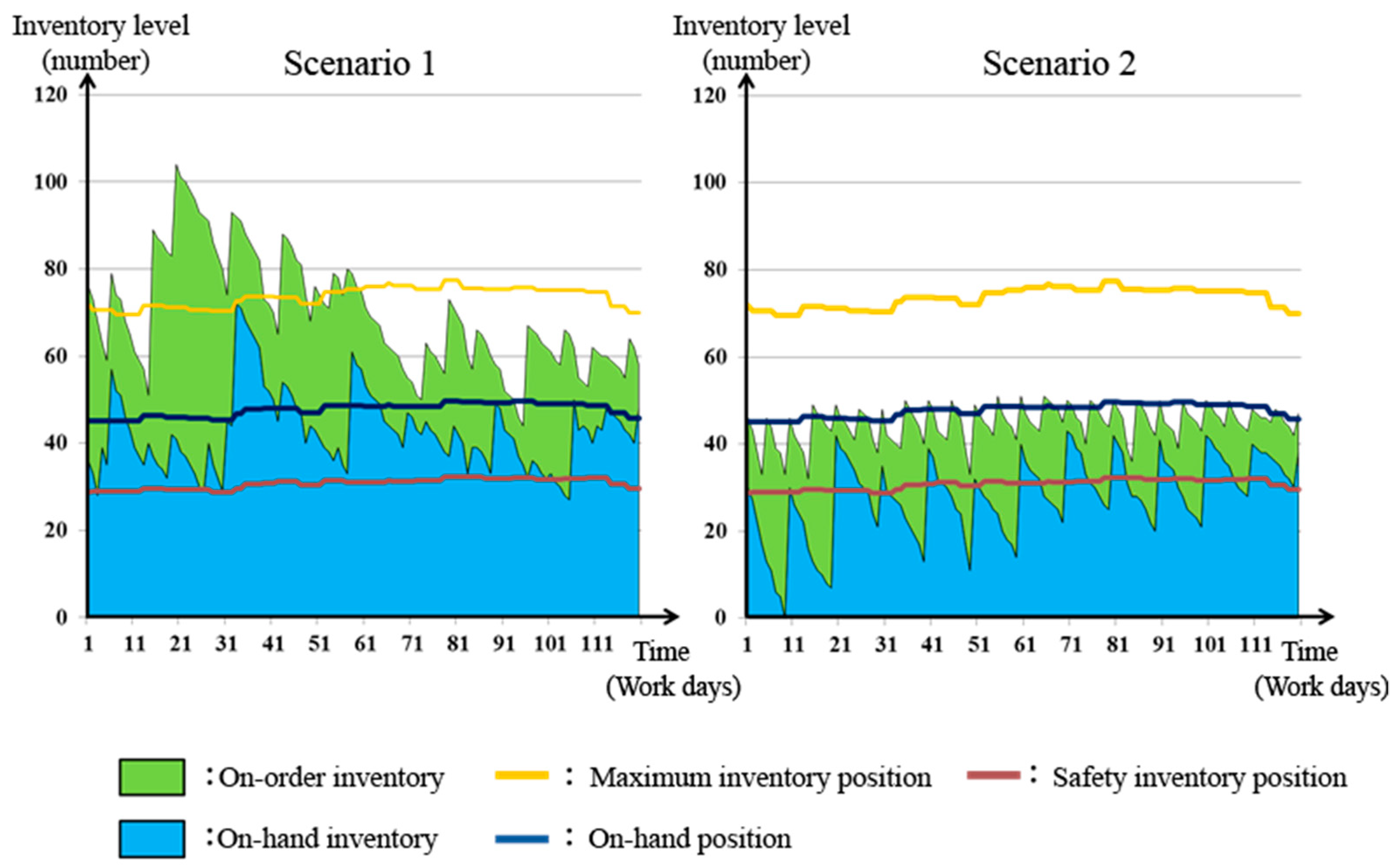
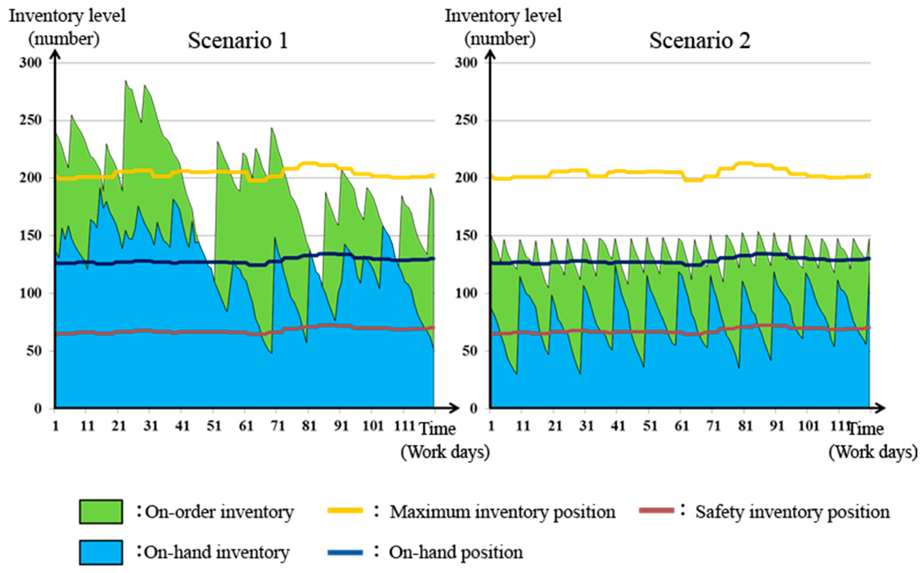
In this study, we performed an analysis based on the DC warehouse. As this research has a total of 20 parts, only one part provided by the four suppliers were included in the inventory status chart, with a time period of 120 working days. We also compared Scenario 1 to our proposed four- item model through analysis of the indicator lines on the chart.

Five types of information are presented in the chart: the accumulation of inventory and the indicator lines.

• The quantity of merchandise that has been shipped from the DC warehouse;
• The quantity of inventory currently located at the DC warehouse;
• The maximum quantity of inventory, which is illustrated as an indicator line, is equal to the total quantity that has been shipped and the quantity in inventory. Therefore, if the total amount of these two quantities is higher than the indicator line; this implies that the warehouse is overstocked;
• The safe inventory quantity, which is represented by an indicator line, occurs when the quantity of the inventory is lower than the indicator line. This implies that an urgent order for inventory is required. However, when the inventory is lower than this indicator line for a long period of time, warehouse workers must check if there has been any problem with the ordering or manufacturing process.
• Inventory quantity, which is denoted by an indicator line, represents the peak value of the inventory and is a gauge of the capacity of the warehouse.

In this study, the three indicators of Scenario 1 were applied to the Scenario 2 model comparing the indicator line of the Scenario 1 and the diagram of the quantity of shipped merchandise in the inventory. We also analyzed the difference between Scenario 1 and the inventory quantity using the Scenario 2 model. It also described the advantages of the Scenario 2 model.

3.1. Comparison and Analysis of the Data Chart

As shown in Figure 4, the original inventory status data indicates that the cumulative on-order and on-hand inventory in Scenario 1 often exceeded the maximum inventory position line, particularly on the work days of 46~53, which signifies a substantial decline in stock without purchase order refills. Moreover, the on-hand inventory was not consistent with the on-order stock which fluctuated significantly. As shown in the diagram, substantial declines occurred on work days 41~61. It also indicates that the safety inventory was set as “used only during work days 51–61”.

Furthermore, Figure 4 shows the inventory level mapping after substituting the parts data in the Scenario 2 mathematical model, which shows a more stable inventory status than in the other scenario. Compared to the maximum inventory position of the cumulative on-order and on-hand inventory, Scenario 1 shows that the inventory level in this study was much lower compared to Scenario 2. Hence, in Scenario 2, the mathematical model, the quantity of the required parts in stock in the supply chain was also lower compared to Scenario 1. The on-hand inventory in Scenario 2 was also more consistent with the on-hand inventory position line of Scenario 1, indicating that the model in this study was more consistent with the indicator line set in the actual situation. In addition, with regard to the safety inventory, the model was able to help workers quickly respond when the on-hand inventory dropped lower than the indication line by pulling back the on-hand inventory to the on-hand inventory position. Therefore, it can be concluded that the model under study and the purpose of setting the safety inventory indicatory line based on the actual situation were more consistent with each other.

In addition to the reduced inventory costs presented by the data, since the on-hand inventory in the Scenario 2 model was stable, the distribution center employees (warehouse) can determine exactly how much space to set aside for the parts. Compared to the instability of Scenario 1, the inventory space demand of the Scenario 2 model will continually require less space, which corresponds to lower inventory costs.

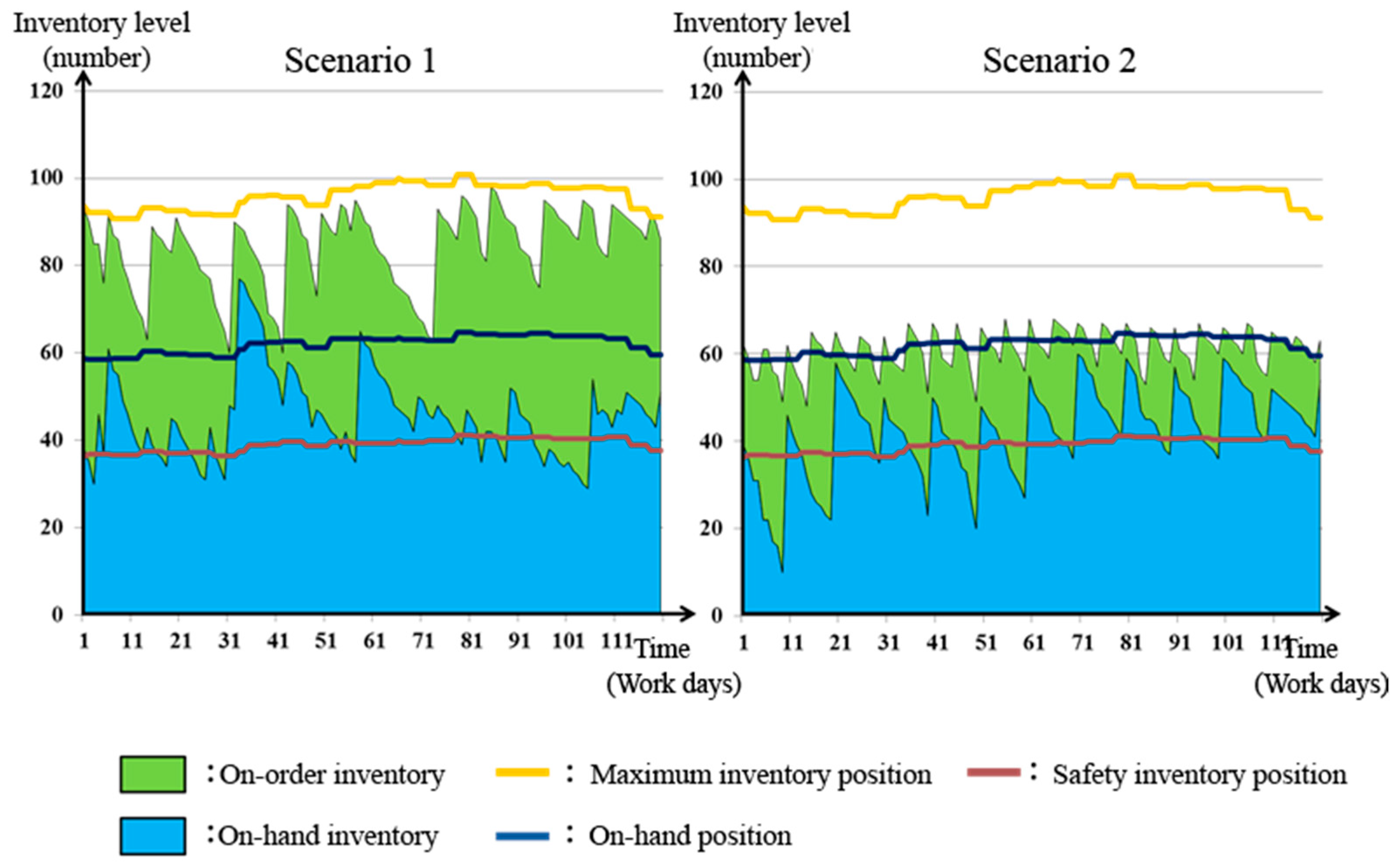
As shown in Figure 5, the original inventory status data indicate that the cumulative on-order and on-hand inventory of Scenario 1 was not at all consistent with the maximum inventory position line, which was often higher or lower than the other indicators. This shows a problem with the parts inventory. Moreover, the on-hand inventory was not consistent with the inventory position. It fluctuated between high and low, specifically during several sections of work days that were much higher than the on-hand inventory position. Conversely, the safety inventory of the parts was not utilized very often. The diagram shows that the safety inventory was only used for six days, causing a backlog of inventory.

After substituting the parts data in the mathematical model in Scenario 2, Figure 5 shows that the inventory status was more stable. When we compare the on-order inventory to that on-hand and the maximum inventory position line of Scenario 1, the inventory in Scenario 2 is seen to be much lower than that of Scenario 1. Therefore, under the mathematical model in scenario 2, the quantity of parts needed to be stocked in the supply chain was lower compared to that of Scenario 1. However, inventory in Scenario 2 was more consistent with the on-hand inventory position line in Scenario 1, indicating that the model in this study better meets the indication line set in Scenario 1. Although the peak value of the on-hand inventory failed to meet the on-hand inventory position set in Scenario 1, the safety inventory in the Scenario 2 model compared to the Scenario 1 shows that the parts were used. Therefore, it can be concluded that the on-hand inventory peak value in the Scenario 2 model was not at all consistent with the on-hand position set in the actual situation because the on-hand inventory and safety inventory position set in Scenario 1 was too high. Hence, according to our findings, the new on-hand inventory position and the inventory position modeled in Scenario 2 was much more effective.

In addition to reducing inventory costs, since the on-hand inventory in the Scenario 2 model was stable, the distribution center employees (warehouse) will know exactly how much space to set aside for the inventory parts. Compared to the instability of Scenario 1 and Scenario 2 requires much less space, thus lowering inventory costs.

The original inventory status data of parts number 3-1, seen in Figure 6, shows that the cumulative on-order and on-hand inventory of Scenario 1 were not at all consistent with the maximum inventory position line, which was often higher or lower than the indicators with a large gap. This signifies a problem with the parts inventory. In addition, the on-hand inventory parts were completely inconsistent with the on-hand inventory position. The diagram shows that at 1~48 work days, it was higher than the on-hand inventory, and the safety inventory was infrequently used. The diagram also shows this with the safety inventory set at 120 work days. The on-hand inventory was lower than the safety inventory’s position only at three stages, indicating that the safety inventory was only used three times. Thus, we can conclude that this scenario suffers from an excessive number of inventory parts.

Figure 6 shows the inventory map after substituting the parts data in the mathematical model in Scenario 2. This indicates that the inventory status examined in this study was more stable. The cumulative on-order and on-hand inventory, which was compared to the maximum inventory position line of Scenario 1, show that the inventory in this study was much lower than in Scenario 1. Therefore, under the mathematical model in Scenario 2, the number of parts needed to be stocked in the supply chain was lower than in Scenario 1. Conversely, the on-hand inventory in Scenario 2 was more consistent with the on-hand inventory position line in Scenario 1, indicating that the model in this study better meets the indication line set in the actual situation. In addition, with regard to the safety inventory, the model was able to help employees quickly respond when the on-hand inventory dropped lower than the indication line by pulling back the on-hand inventory to the on-hand inventory position. Therefore, it can be concluded that the model in this study and the purpose of setting the safety inventory indicatory line based on the actual situation are more consistent with each other.

In addition to the reduced inventory costs presented by the data, since the on-hand inventory in the Scenario 2 model was stable, the distribution center (warehouse) employees can determine exactly how much space to set aside for the parts. Compared to the instability of Scenario 1, the space required for inventory in the Scenario 2 model was significantly reduced, thus lowering the inventory costs.

The original inventory status data of parts number 4-1, as shown in Figure 7, indicate that the on-hand inventory was not consistent with the on-hand position. This was due to the fact that the on-hand inventory had not been replenished to the on-hand position for a long time; however, the on-hand inventory peak values only exceeded the on-hand position three times. Moreover, the safety inventory of the parts was low. The diagram shows that there were roughly 40 safety inventory indicator lines and the minimum on-hand inventory of the parts within 120 work days was 29, indicating that the safety inventory indicators had been set too high.

After substituting the parts data in the mathematical model in Scenario 2, the inventory mapping, seen in Figure 7, indicates that the inventory status was more stable than in Scenario 1. When we compared the cumulative on-order and on-hand inventory to the maximum inventory position in Scenario 1, we found the inventory in Scenario 2 to be much lower. In contrast, the on-hand inventory in Scenario 2 was more consistent with the on-hand inventory position in Scenario 1, indicating that the model in this study was more in line with the indicator lines set in the actual situation. Additionally, whenever the on-hand safety inventory in Scenario 2 dropped below the indicator line, the employees were able to quickly move the on-hand inventory back to the correct inventory position. Hence, the model in Scenario 2 was more effective for setting up the safety inventory indicator lines.

Table 4. The inventory in Scenario 1 and of the corresponding manufacturers in Scenario 2.

Number of Manufacturing Suppliers	Scenario 1	Scenario 2	Reducing
	Distribution Center (Warehouse Inventory)	Distribution Center (Warehouse Inventory)
1	41,574	27,113	35%
2	25,718	10,409	60%
3	74,354	45,760	38%
4	26,480	24,116	9%
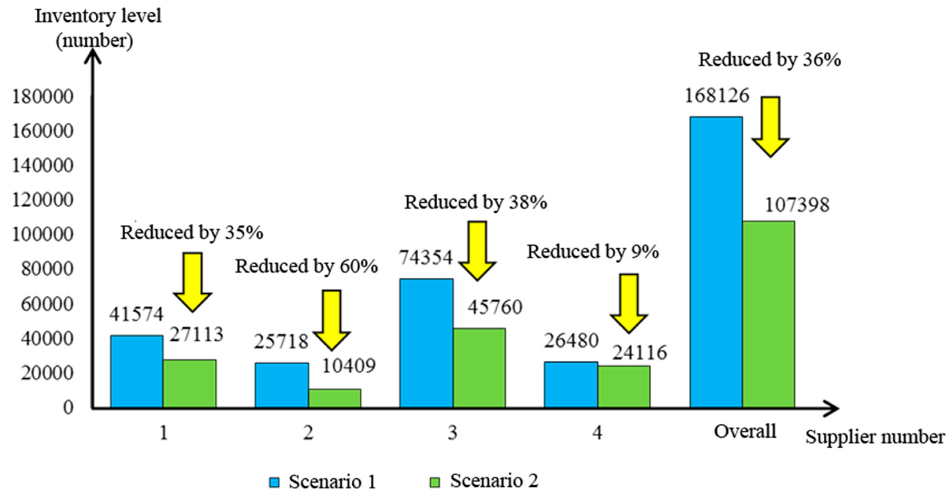
Overall	168,126	107,398	36%

and Figure 8 show the statistical inventory and the corresponding manufacturers in Scenario 2 as well as the inventory of Scenario 1 in the DC warehouse. It is clear that the inventory of parts provided by manufacturer 1 is reduced by 35% in the Scenario 2 model; the inventory of parts provided by manufacturer 2 is reduced by 60% in this model; the inventory of parts provided by manufacturer 3 is reduced by 38% in this model; the inventory of parts provided by manufacturer 4 is reduced by 9% in the Scenario 2 model. Overall, this model shows a 36% reduction, which indicates that the inventory in Scenario 2 is indeed lower than it was in Scenario 1. Therefore, this model will help warehouse managers to significantly reduce their inventory compared to Scenario 1. The manufacturers of 1 and 3 reduced inventory by 35% and 38%, respectively. Manufacturer 2 had the highest rate of reduction at 60%.

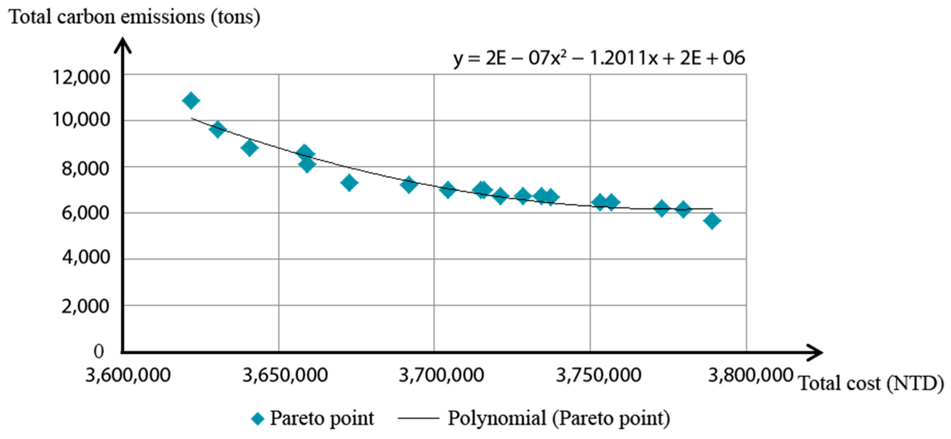
We resolved and found 20 Pareto points after filtering out the inappropriate solutions which are shown in

Table 5. Pareto points for total carbon emissions and total cost.

Pareto Point	Total Cost (NTD)	Total Carbon Emissions (Tons)	Scenario 1 Rate	Scenario 2 Rate
1	3,788,938	5643.84	100%	0%
2	3,779,792	6139.62	90%	10%
3	3,773,009	6183.89	90%	10%
4	3,756,896	6424.73	85%	15%
5	3,753,054	6428.43	85%	15%
6	3,737,442	6651.47	80%	20%
7	3,734,557	6687.07	80%	20%
8	3,728,580	6695.74	80%	20%
9	3,721,358	6709.84	80%	20%
10	3,716,113	6950.68	75%	25%
11	3,714,874	6954.38	75%	25%
12	3,704,433	6980.86	75%	25%
13	3,692,042	7177.42	70%	30%
14	3,672,707	7280.07	70%	30%
15	3,659,275	8068.36	55%	45%
16	3,658,987	8516.16	45%	55%
17	3,658,454	8560.44	45%	55%
18	3,640,775	8804.98	40%	60%
19	3,630,660	9573.50	25%	75%
20	3,622,008	10,841.50	0%	100%

. As shown in Figure 9, using total carbon emissions as the X-axis and total cost as the Y-axis, the total carbon emissions of the Pareto points 16~20 increased significantly; however, the total cost reduction was higher. The 20 Pareto points in Scenario 1 had a much higher usage ratio of over 50% than those in Scenario 2, which were only 15:5. Therefore, the Pareto points are less obvious when they are closest to their highest point and if the usage ratio in Scenario 2 is higher than 50%. As shown in Figure 9, the distribution condition of the Pareto points chosen for this study corresponds to the Pareto boundary solution proposed by Messac et al. [30]. (The formula is: y = 2E − 07x² − 1.2011x + 2E + 06)

3.2. Comparison to the Traditional Supply Chain

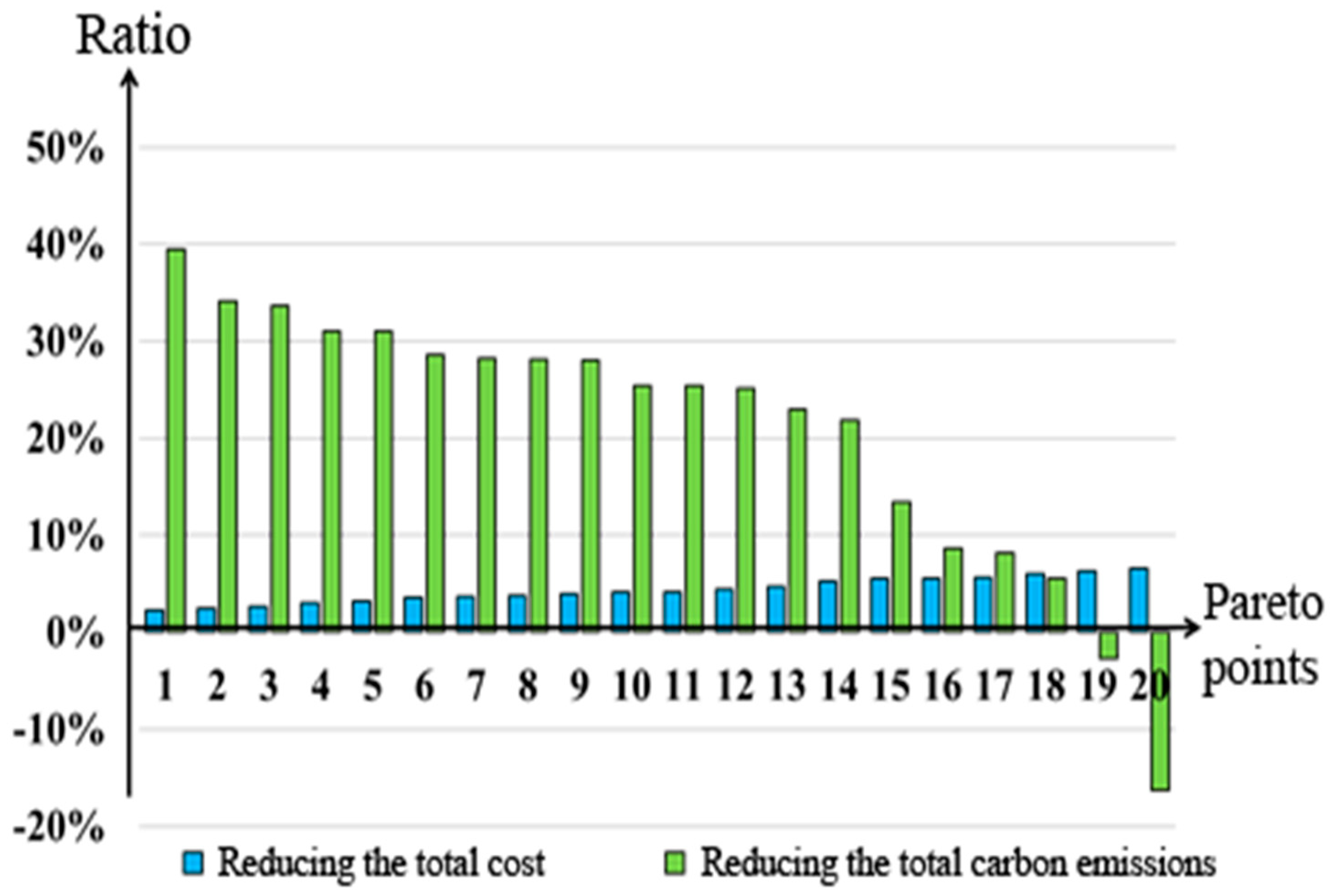
In the traditional supply chain, the return journey of empty vehicles from the DC warehouses to the retailers is not considered. The total cost of Scenario 1 in the traditional supply chain is 3,875,518 (dollars), and the total carbon emissions are 9319.44 (tons).

Table 6. Comparison of total cost and carbon emissions between the Pareto points and the traditional supply chain.

Pareto Point	Total Cost (NTD)	Total Carbon Emissions (Tons)	Total Cost Reduction	Total Carbon Emissions Reduction
1	3,788,938	5643.84	2.23%	39.44%
2	3,779,792	6139.62	2.47%	34.12%
3	3,773,009	6183.89	2.65%	33.65%
4	3,756,896	6424.73	3.06%	31.06%
5	3,753,054	6428.43	3.16%	31.02%
6	3,737,442	6651.47	3.56%	28.63%
7	3,734,557	6687.07	3.64%	28.25%
8	3,728,580	6695.74	3.79%	28.15%
9	3,721,358	6709.84	3.98%	28.00%
10	3,716,113	6950.68	4.11%	25.42%
11	3,714,874	6954.38	4.15%	25.38%
12	3,704,433	6980.86	4.41%	25.09%
13	3,692,042	7177.42	4.73%	22.98%
14	3,672,707	7280.07	5.23%	21.88%
15	3,659,275	8068.36	5.58%	13.42%
16	3,658,987	8516.16	5.59%	8.62%
17	3,658,454	8560.44	5.60%	8.14%
18	3,640,775	8804.98	6.06%	5.52%
19	3,630,660	9573.50	6.32%	−2.73%
20	3,622,008	10,841.50	6.54%	−16.33%

and Figure 10 show a comparison of Scenario 1 in the traditional supply chain to the 20 Pareto points obtained by Scenario 1 and 2 models for this study. Pareto point 1 can reduce the most carbon emissions by 39.44% and has the least total cost of 2.23%. When comparing this data with Table 5, we can see that the Pareto points use 100% in the Scenario 1 model. From the data, it is clear that Scenario 1 model shows a significant reduction in carbon emissions and a small reduction in total cost, compared to the traditional supply chain. With the higher usage ratio, shown in the Scenario 2 model, the Pareto points indicate a slight increase in both carbon emissions and total cost. For example, from the 15th Pareto point, the reduction ratio of carbon emissions decreases rapidly, however, the reduction ratio of the total cost is more gradual.

Compared to the traditional supply chain, we discovered that Scenario 1 and 2 models indicate significant improvements in the carbon emissions and total cost throughout the supply chain. Furthermore, we can utilize the usage ratio of Scenarios 1 and 2 to choose the most efficient expectation value, creating more options for the new transportation model in the supply chain. Moreover, the new transportation model of the supply chain can be used to reduce the carbon emissions and total cost, which results in an increase in the additional transportation cost. Therefore, the competitiveness of our Scenario 1 model is enhanced and the transportation pattern in the Scenario 2 model is able to provide a more stable and smaller inventory for the DC warehouse. The Scenario 2 model indeed has the effect of improving the inventory status at an overall reduction rate of 36%. However, the more realistic increase in transportation cost does not offset money saved from the inventory reduction.

The increase in transportation distance also increases carbon emissions. Therefore, compared to the traditional supply chain, the higher usage and additional transportation of the Scenario 2 model indicates higher carbon emissions in the supply chain of the total cost and total carbon emissions.

4. Conclusions and Future Research

In this study, two models were constructed to ensure sustainability for the traditional supply chain. The analysis in Section 3.1 shows that the mathematical model in Scenario 2 proposed in this study can ensure better sustainability compared to that of the traditional supply chain status. In particular, Pareto points 1–18 were superior to the traditional supply chain in terms of total cost and total carbon emissions. Clearly, the scenarios analyzed in this study show significant improvement results. The model in Scenario 1 used return vehicles to carry out reverse logistics in an attempt to ensure a greener and more sustainable supply chain. The model in Scenario 2 used return vehicles to reduce the lead time from the manufacturing supplier to the distribution center (warehouse), which led to greater inventory stability at the distribution center (warehouse) and reduced inventory levels.

With the goal of minimizing costs and carbon emissions, the role of return vehicles was explored under two different scenarios. A four-level supply chain model was also established to serve as the basis of the supply chain. A more effective inventory system was proposed to not only reduce costs and ensure a greater inventory stability, but also to make sure that the inventory status was consistent with the indicator lines of Scenario 1. In addition, the recycling and reuse of packaging material as it pertains to reverse logistics was analyzed to determine how to reduce carbon emissions throughout the entire supply chain. Finally, based on the data analysis of the case study, two conclusions are summarized as 1. The Scenario 2 model has a superior inventory status, with an overall reduction rate of 36%, which proves that a higher delivery frequency and the reduction of lead time are able to create an even more efficient inventory status. Therefore, we encourage business executives to refer to the mathematical models proposed in this research paper when they look for options to reduce inventory. They can plug the statistical data into the mathematical models to obtain the Pareto points and the percentage of inventory reduction. In Section 3 of our paper, we discuss the role of two key elements: the environment and the economy. In our scenario models, there are 18 Pareto points that reduce both the cost and carbon emissions, which creates a win-win situation for the company. From these results, it can be concluded that this research provides better alternatives to the traditional supply chain. Business executives will be able to choose from these 18 different options and find the most suitable solution for their companies. 2. Allowing returning vehicles to carry packing material for reverse logistics recycling not only resolves the issue of returning empty vehicles but also resolves the transportation vehicle issue in reverse logistics, which creates yet another win-win situation. In this model, the transportation vehicle is the key component of forwarding logistics in the supply chain when delivering merchandise and in the reverse logistics on its return journey. Thus, vehicles using this model can carry out the function of both forward and reverse logistics, minimizing the possibility of empty vehicle transportation. This transportation model can be utilized to reduce carbon emissions from the recycling of packing materials within the manufacturing process and in vehicle transportation.

This study sought to arrive at an optimal policy regarding carbon emsisions and materials recovery objectives. We include additional considerations in the scope of green and sustainable topics to this multi-objective problem. The environmental concerns are a recommended future direction for research [31].

In addition, while open-loop recycling networks with minimal levels are favored due to their relatively high recycling equipment investment costs, varying the recycling network model to arrive at a more realistic consideration can also be accomplished by altering the number of facilities, their relative distances from each other, and their individual capacities [32]. To arrive at an optimal solution for the extended carbon-capped network with multiple echelons, the JIT NP-hard problem requires a metaheuristic approach, such as a genetic algorithm method [33].

Furthermore, the analysis on current reverse logistics trends suggests that future research regarding supply chain networks should employ increased levels of complexity to match specific business conditions [34]. Empirical research, such as case studies, interviews, and analyses, could also be used to assess the effectiveness of the reverse logistics strategies used in specific organizations, in addition to proposing alternative models for improvement.

References

- Lu, L.Y.; Wu, C.; Kuo, T.-C. Environmental principles applicable to green supplier evaluation by using multi-objective decision analysis. Int. J. Prod. Res. 2007, 45, 4317–4331. [Google Scholar] [CrossRef]
- Cucchiella, F.; Koh, L.; Björklund, M.; Martinsen, U.; Abrahamsson, M. Performance measurements in the greening of supply chains. Supply Chain Manag. Int. J. 2012, 17, 29–39. [Google Scholar]
- Porter, M.E.; Van der Linde, C. Toward a new conception of the environment-competitiveness relationship. J. Econ. Perspect. 1995, 9, 97–118. [Google Scholar] [CrossRef]
- Srivastava, S.K. Green supply-chain management: A state-of-the-art literature review. Int. J. Manag. Rev. 2007, 9, 53–80. [Google Scholar] [CrossRef]
- Wang, F.; Lai, X.; Shi, N. A multi-objective optimization for green supply chain network design. Dec. Support Syst. 2011, 51, 262–269. [Google Scholar] [CrossRef]
- Green, K.W., Jr.; Zelbst, P.J.; Meacham, J.; Bhadauria, V.S. Green supply chain management practices: Impact on performance. Supply Chain Manag. Int. J. 2012, 17, 290–305. [Google Scholar] [CrossRef]
- Herold, D.M.; Farr-Wharton, B.; Lee, K.H.; Groschopf, W. The interaction between institutional and stakeholder pressures: Advancing a framework for categorising carbon disclosure strategies. Bus. Strategy Dev. 2019, 2, 77–90. [Google Scholar] [CrossRef]
- Herold, D. Has carbon disclosure become more transparent in the global logistics industry? An investigation of corporate carbon disclosure strategies between 2010 and 2015. Logistics 2018, 2, 13. [Google Scholar] [CrossRef]
- Tognetti, A.; Grosse-Ruyken, P.T.; Wagner, S.M. Green supply chain network optimization and the trade-off between environmental and economic objectives. Int. J. Prod. Econ. 2015, 170, 385–392. [Google Scholar] [CrossRef]
- Fahimnia, B.; Sarkis, J.; Boland, J.; Reisi, M.; Goh, M. Policy insights from a green supply chain optimisation model. Int. J. Prod. Res. 2015, 53, 6522–6533. [Google Scholar] [CrossRef]
- Li, S.; Jayaraman, V.; Paulraj, A.; Shang, K.-C. Proactive environmental strategies and performance: Role of green supply chain processes and green product design in the Chinese high-tech industry. Int. J. Prod. Res. 2016, 54, 2136–2151. [Google Scholar] [CrossRef]
- Gu, Y.; Wu, Y.; Xu, M.; Mu, X.; Zuo, T. Waste electrical and electronic equipment (WEEE) recycling for a sustainable resource supply in the electronics industry in China. J. Clean. Prod. 2016, 127, 331–338. [Google Scholar] [CrossRef]
- Wei, C.; Li, Y.; Cai, X. Robust optimal policies of production and inventory with uncertain returns and demand. Int. J. Prod. Econ. 2011, 134, 357–367. [Google Scholar] [CrossRef]
- Mitra, S. Inventory management in a two-echelon closed-loop supply chain with correlated demands and returns. Comput. Ind. Eng. 2012, 62, 870–879. [Google Scholar] [CrossRef]
- Govindan, K.; Paam, P.; Abtahi, A.-R. A fuzzy multi-objective optimization model for sustainable reverse logistics network design. Ecol. Ind. 2016, 67, 753–768. [Google Scholar] [CrossRef]
- Zikopoulos, C.; Tagaras, G. Reverse supply chains: Effects of collection network and returns classification on profitability. Eur. J. Oper. Res. 2015, 246, 435–449. [Google Scholar] [CrossRef]
- Nassani, A.A.; Aldakhil, A.M.; Abro, M.M.Q.; Zaman, K. Environmental Kuznets curve among BRICS countries: Spot lightening finance, transport, energy and growth factors. J. Clean. Prod. 2017, 154, 474–487. [Google Scholar] [CrossRef]
- Du, F.; Evans, G.W. A bi-objective reverse logistics network analysis for post-sale service. Comput. Oper. Res. 2008, 35, 2617–2634. [Google Scholar] [CrossRef]
- Skjoett-Larsen, T. Third party logistics–from an interorganizational point of view. Int. J. Phys. Distrib. Logist. Manag. 2000, 30, 112–127. [Google Scholar] [CrossRef]
- Evangelista, P.; Santoro, L.; Thomas, A. Environmental sustainability in third-party logistics service providers: A systematic literature review from 2000–2016. Sustainability 2018, 10, 1627. [Google Scholar] [CrossRef]
- Motor, H. Yangmei Logistic Center. Available online: https://pressroom.hotaimotor.com.tw/zh/article/00115 (accessed on 23 October 2019).
- McKinnon, A.; Edwards, J. Opportunities for improving vehicle utilization. In Green Logistics: Improving the Environmental Sustainability of Logistics; Kogan Page: London, UK, 2010; pp. 195–213. [Google Scholar]
- Hsu, C.-C.; Tan, K.-C.; Mohamad Zailani, S.H. Strategic orientations, sustainable supply chain initiatives, and reverse logistics: Empirical evidence from an emerging market. Int. J. Oper. Prod. Manag. 2016, 36, 86–110. [Google Scholar] [CrossRef]
- Kapetanopoulou, P.; Tagaras, G. Drivers and obstacles of product recovery activities in the Greek industry. Int. J. Oper. Prod. Manag. 2011, 31, 148–166. [Google Scholar] [CrossRef]
- Zhu, Q.; Sarkis, J.; Lai, K.-H. Examining the effects of green supply chain management practices and their mediations on performance improvements. Int. J. Prod. Res. 2012, 50, 1377–1394. [Google Scholar] [CrossRef]
- Raghunathan, S.; Yeh, A.B. Beyond EDI: Impact of continuous replenishment program (CRP) between a manufacturer and its retailers. Inf. Syst. Res. 2001, 12, 406–419. [Google Scholar] [CrossRef]
- Ayers, J.B. Handbook of Supply Chain Management; Auerbach Publications: Boca Raton, FL, USA, 2006. [Google Scholar]
- Cachon, G.; Fisher, M. Campbell soup’s continuous replenishment program: Evaluation and enhanced inventory decision rules. Prod. Oper. Manag. 1997, 6, 266–276. [Google Scholar] [CrossRef]
- Schenck, J.; McInerney, J. Applying vendor-managed inventory to the apparel industry. Autom. ID News 1998, 14, 36–38. [Google Scholar]
- Messac, A.; Ismail-Yahaya, A.; Mattson, C.A. The normalized normal constraint method for generating the Pareto frontier. Struct. Multidiscip. Optim. 2003, 25, 86–98. [Google Scholar] [CrossRef]
- Govindan, K.; Soleimani, H.; Kannan, D. Reverse logistics and closed-loop supply chain: A comprehensive review to explore the future. Eur. J. Oper. Res. 2015, 240, 603–626. [Google Scholar] [CrossRef]
- Agrawal, S.; Singh, R.K.; Murtaza, Q. A literature review and perspectives in reverse logistics. Resour. Conserv. Recycl. 2015, 97, 76–92. [Google Scholar] [CrossRef]
- Memari, A.; Rahim, A.R.A.; Absi, N.; Ahmad, R.; Hassan, A. Carbon-capped distribution planning: A JIT perspective. Comput. Ind. Eng. 2016, 97, 111–127. [Google Scholar] [CrossRef]
- Wang, J.-J.; Chen, H.; Rogers, D.S.; Ellram, L.M.; Grawe, S.J. A bibliometric analysis of reverse logistics research (1992–2015) and opportunities for future research. Int. J. Phys. Distrib. Logist. Manag. 2017, 47, 666–687. [Google Scholar] [CrossRef] [Green Version]
Figure 1.
Diagram of the addition of return vehicles in a typical logistics supply chain.
Figure 2.
Supplier chain transportation in Scenario 1. (Source: Compilation from this study).
Figure 3.
Supply chain transportation of goods in Scenario 2. (Source: Compilation for this study).
Figure 4.
Inventory status of part 1 in Scenarios 1 and 2. (Source: Compilation from this study).
Figure 5.
Inventory status of part 2 in Scenarios 1 and 2. (Source: Compilation from this study).
Figure 6.
Inventory status of part 3 in Scenarios 1 and 2. (Source: Compilation from this study).
Figure 7.
Inventory status of part 4 in Scenarios 1 and 2. (Source: Compilation from this study).
Figure 8.
Inventory levels of Scenario 1 and corresponding manufacturing supplier numbers under Scenario 2. (Source: Compilation from this study).
Figure 9.
The distribution diagram of total carbon emissions and total cost.
Figure 10.
Diagram comparing the total cost and carbon emissions between Pareto points and the traditional supply chain.