Article

Optimization of Transportation Routing Problem for Fresh Food by Improved Ant Colony Algorithm Based on Tabu Search

1
Institute of Innovation & Application, Zhejiang Ocean University, Zhoushan 316022, China
2
Research Center of Zhejiang Free Trade (ZhouShan) Zone, School of Economics and Management, Zhejiang Ocean University, Zhoushan 21600, China
3
School of Business Administration, Wonkwang University, Jeonbuk 54538, Korea
*
Authors to whom correspondence should be addressed.
Sustainability 2019, 11(23), 6584; https://0-doi-org.brum.beds.ac.uk/10.3390/su11236584
Submission received: 4 October 2019 / Revised: 12 November 2019 / Accepted: 12 November 2019 / Published: 21 November 2019
(This article belongs to the Section Environmental Sustainability and Applications)

Abstract

:
With the continuous improvement of people’s living standards and their increasing demand for fresh food, the cold chain logistics industry has developed rapidly. One of the biggest challenges to today’s cold chain logistics is to offer fresh food while minimizing CO2 emissions. The fresh degree and CO2 emissions are involved in the vehicle routing optimization problem in the cold chain logistics. In order to meet the quality requirement for fresh agricultural products and low carbon logistics, a novel routing optimization model considering the costs of quality deterioration and carbon emissions (Low Carbon and Freshness Degrees Vehicle Routing Problem (LCFD-VRP)) for cold chain distribution was established in this study. This model takes into account the fixed cost, fuel cost and time window penalty cost. An improved ant colony algorithm (IACA) is used to optimize the whole vehicle distribution routing with its strong global search ability. Tabu Search (TS) algorithm is used to search the single vehicle distribution routing with its good local search ability. An IACA combined with TS (IACATS) was proposed to solve the above LCFD-VRP model. The practicability of the model and the effectiveness of the above improved algorithm are verified using a real case study. The results of Zhoushan Dayang Refrigerated Logistics Co., Ltd. showed that, compared with the traditional algorithm, IACATS could reduce the dispatching of two refrigerated vehicles, thus lowering the total cost by 4.94%, shortening the actual transportation distance by 5.50% and cutting the total CO2 emissions by 8.9%. Therefore, the LCFD-VRP model can effectively help to achieve the low carbon emissions, multi-variety and low-cost distribution of fresh agricultural products. The proposed model and IACATS algorithm would be used to optimize VRP in cold chain enterprises. The results of this study also provide management suggestions for cold chain enterprises to effectively balance economic cost and environmental cost.

1. Introduction

With the development of the economy and the improvement in people’s life quality, green and healthy products have gradually become the primary standard for consumers to choose fresh foods [1]. This has resulted in the rapid development of global fresh agricultural products via cold chain logistics around the world. Compared with traditional logistics, the cold chain logistics of agricultural products has higher requirements for quality and timeliness [2]. The normal operation of refrigeration equipment produces a large amount of CO2 emissions and other greenhouse gases generated from distribution vehicles in the process of delivery. It leads to an increase in greenhouse gases and, as a result, air pollution and greenhouse effect will be intensified. The increased carbon emissions not only pollute the environment, but also raise the cost of logistics enterprises due to the implementation of national carbon-taxing policies [3]. Therefore, how to reduce carbon emissions in cold chain logistics, thereby alleviating the global warming caused by the greenhouse effect, has become a popular issue in the research field of cold chain logistics distribution routes [4].
In recent years, the optimization of cold chain logistics distribution routes has attracted extensive academic attention [5,6]. Although the above-mentioned studies have considered the impacts of various cost factors on cold chain logistics, there is still little research on cold chain logistics that considers the three factors of economy, product freshness, and environment at the same time [7]. Therefore, further studies should focus on how to construct suitable model to minimize cost coupling with increasing of product freshness and decreasing carbon emissions in the model according to the real situations. Considering the number of nodes explosively increase in cold chain logistics, how to design more effective algorithms to improve the efficiency of solutions to the model of the problem is of great urgency. More importantly, the practicability of the model and the effectiveness of the algorithm need to be verified by real cases.
We herein propose a comprehensive Low Carbon and Freshness Degrees Vehicle Routing Problem (LCFD-VRP) model to optimize vehicle routing. This aims to minimize total costs, including the carbon emissions costs, and to maximize product freshness, based on the strategy of cost–benefit. The potential challenges in finding the solution of LCFD-VRP using improved ant colony algorithm combined with tabu search (IACATS) are as follows: (1) what are the essential attributes in the routing optimization? (2) How does the IACATS synergetic handle all the vehicles and the single vehicle in short time? (3) How are the simulated results evaluated? By means of IACATS algorithm, we used the strong global search ability of the improved ant colony algorithm to optimize the overall vehicle routing, and the local optimization ability of the tabu search (TS) algorithm to solve the local search of a single vehicle distribution route in the constructed LCFD-VRP model. The LCFD-VRP and IACATS algorithm were verified through a case study of the distribution service of fresh agricultural products provided by Zhoushan Dayang Refrigerated Logistics Co., Ltd. in Zhoushan, Zhejiang Province, which fits more with the real enterprise operations. It also achieved the three win–win situation among economic, environmental benefits and personal health demand.
Thus, the remainder of this paper is organized as follows: a literature review is presented in Section 2. The model formulation is proposed in Section 3. An improved ant colony algorithm and TS algorithm is described in Section 4. The algorithm construction and case study are shown in Section 5. The results are illustrated in Section 6. The short discussion and the outlook for future research are presented in Section 7. Finally, the conclusions of this paper are listed in Section 8. The schematic illustration of this paper can be expressed as follows (Figure 1).

2. Literature Review

This paper mainly aims to obtain an optimal distribution plan with consideration of the fresh degree and carbon emissions in cold chain logistics distribution. By reviewing the previous research literature [8,9,10,11], we have found that the academic research on this issue can be divided into the following four fields: VRP model in cold chain logistics, VRP with freshness degree, VRP with carbon emissions and optimization algorithms.

2.1. Research Considering the VRP Model in Cold Chain Logistics

VRP has been treated as one of the most important theoretical and practical problems in mathematical and logistics fields since it was first proposed by Danttzig and Ramser in 1959 [12]. VRP can be classified into many sub-problems according to the different situation mathematical and logistics fields [13]. Many experts have focused on the fuel consumption model and the instant fuel consumption model in cold chain logistics [14]. Hsiao et al. [15] stated the relationship between the speed and load of the vehicle as well as its fuel consumption to establish the fuel consumption model in cold chain logistics. It can be concluded that running time is an engine-related module with a linear mathematical relationship among the total weights of the vehicle and velocity. Cheng et al. [16] considered the travel distance, the speed of the car, the load of the vehicle, etc., assuming that a bigger load M (mass) of the vehicle would increase p (speed). In regards to the instant fuel consumption model in cold chain logistics, Zhang et al. [17] considered the vehicle’s characteristics, such as weight, travel speed and acceleration, and established the vehicle instantaneous fuel consumption model in cold chain logistics. Many scholars have further constructed high quality derived models and relative heuristic algorithms for identification in cold chain logistics [18,19,20]. For instance, they investigated the influence of time window constraints in the process of cold chain logistics distribution–route optimization [21]. Anderson et al. [22] further explored the vehicle routing problem with time windows under the indistinct customer demand and established a multi-objective indistinct probability constrained programming model for minimizing vehicle travel distance and delivery service delay in cold chain logistics. Chung et al. [23] fuzzified the demand and driving time, and constructed a chance-constrained pre-optimization model of variable compensation with regard to time window constraints. Qin et al. [24] optimized cold chain vehicle routing with the objective of minimizing vehicle travel distance and CO2 emissions. Even though many experts and scholars achieved fruitful achievements in the VRP issue in the past several decades, by reviewing the previous literature, we draw the conclusion that the academic research of VRP in cold chain logistics is relatively sufficient. What remains to be proved is that VRP has extensive application value in cold chain logistics.

2.2. Research Considering Fresh Degrees

Because of the perishability of products in cold chain logistics, customers have certain requirements for product freshness. In order to improve customer satisfaction, the freshness of products should be considered in the optimization of the cold chain logistics distribution route. Wang et al. [25] proposed that the freshness of perishable products should be taken as a criterion when measuring the optimal distribution route, and that the multi-distribution center cold chain vehicle routing problem be studied with the objectives of minimum transportation cost, vehicle travel time and product perishability. Yi et al. [26] introduced the freshness loss coefficient and established a multi-objective optimization model for the fresh agricultural products distribution route by considering customer satisfaction and the total cost. Drezner et al. [27] constructed a multi-distribution center vehicle routing problem model with respect to customer service time and product quality requirements. From the existing VRP model, considering fresh degree is relatively rare.

2.3. Research Considering Carbon Emissions

Due to the specialization of cold chain logistics, more fuel consumption is needed, and a larger amount of carbon emissions is generated in the process of transportation. Therefore, green vehicle routing optimization in terms of carbon emissions has become an important field of research. Recently, many scholars have begun to pay attention to VRP models considering carbon emissions. Ghannadpour et al. [28] used a multi-objective dynamic vehicle routing problem with fuzzy travel times and customer satisfaction to study the impact of carbon tax on carbon emissions in the cold chain distribution process. Then, Wang et al. [29] employed an adaptive genetic algorithm combined with greedy algorithm to investigate the impact of carbon tax on carbon emissions in an inventory routing problem. Shen et al. [30] explored the adaptive genetic algorithm, which can dynamically adjust the crossover and mutation probability, to survey the impact of the carbon trading mechanism on carbon emissions in multi-depot open VRP. Niu et al. [31] proposed a green open VRP with time windows by minimizing the comprehensive routing cost, including the fuel cost, carbon emissions cost and driver cost. Guo et al. [32] put forward a hybrid meta-heuristic algorithm to solve the on-line VRP for minimizing costs related to economy and emissions. Naderipour et al. [33] brought forth a cost function, including the driver cost and fuel cost in the time-dependent pollution-routing problem. Liao et al. [34] proposed a new comprehensive model for the measurement, evaluation and minimization of CO2, NOx and CO as three major gas emissions in the open time-dependent vehicle routing problem. Liu et al. [35] proposed a method for calculating carbon emissions and established an integer programming model based on the load and working time constraints of the open pollution routing problem. Fornell et al. [36] investigated the vehicle travel time and carbon emissions, and established a non-linear mixed integer programming model for vehicle scheduling and routing assignment in urban distribution using the improved multi-objective particle swarm optimization algorithm. Zeng et al. [37] taking Zhuhai Express Company as an example, established a distribution route optimization model by treating vehicle load as a factor affecting fuel consumption and CO2 emissions. Parasuraman et al. [38] constructed a distribution route optimization model with the lowest carbon emissions as the objective and based on the necessity of energy saving in cold chain logistics vehicle distribution. Wang et al. [39] considered the differences in energy consumption between the transportation and unloading processes caused by the opening of the refrigerated door, and established the optimal distribution route model of fresh agricultural products in terms of carbon emissions and with the objective of generating the lowest cost.

2.4. Research Considering the Optimization Algorithms

In the mathematical field, VRP is a typical NP (Non-deterministic Polynomial)-hard problem [40]. As the number of nodes increases rapidly, an exact algorithm is rather difficult to employ to solve large scale VRP. Hence, the optimization algorithm could greatly offer help in cold chain logistics enterprises or the individual vehicle drivers, which make them better schedule the vehicle delivery with lower carbon emissions and fuel consumption. On the other hand, it could reduce the operation cost. Currently, it is greatly interesting research fields and has attracted many experts focusing on the research of VRP optimization algorithm [41]. The TS algorithm is a sub-heuristic algorithm that simulates human memory function. It has the characteristics of few parameters, simple structure, and robust global optimization ability [42]. The advantages of TS in real applications have also been demonstrated [43]. Shi et al. [44] created a classic two-step solution algorithm for the multi-trip VRPSD with soft time windows based on TS. Karaoglan et al. [45] designed a dynamic programming based heuristic algorithm for VRP with discrete split deliveries. From the calculated results, their optimization methods had a great effect on reducing carbon emissions and reducing logistics costs [46]. Even though the TS algorithm plays a pivotal role in the heuristic algorithm, it is difficult to use in the global search because of the shortcoming of TS algorithm. The combination with global research algorithm is proved to be an effective method. Li et al. [47] showed that a TS algorithm emerges as the most effective approach. Procedures based on pure genetic algorithms and neural networks are clearly outperformed, while those based on simulated or deterministic annealing and ant systems are not quite competitive. Guo et al. [48] designed a series of TS algorithms to solve the open VRP. They also compared and analyzed some other optimization algorithms, such as simulated annealing algorithm, genetic algorithm, ant colony optimization algorithm, and swarm optimization algorithm.
In summary, few researchers have concerned the three factors of cost, fresh degrees, and environmental pollution within the same model to solve VRP in cold chain logistics. Thus, the carbon emissions and fresh degrees were considered during the vehicle routing optimization in this study. An LCFD-VRP model based on carbon emissions will be established. In addition, the algorithm based on IACA and TS will be proposed to solve LCFD-VRP. The effectiveness of the model and algorithm will be verified by simulating a real example. The simulated results of this study may offer management suggestions for cold chain logistics enterprises to effectively balance economic costs and environmental costs.

3. Model

3.1. Problem Description

The distribution route optimization problem to carbon emissions of fresh agricultural products in the cold chain logistics can be described as follows. A distribution center of fresh agricultural products provides service for multiple customers. Given refrigeration cold chain transporting vehicles of the same type, it starts from the distribution center at a constant speed, stops at each customer point, and returns after completing all distribution tasks. Each location and demand of customers is known, and each customer point is reached by only one vehicle. At the same time, there is the service time constraint. When the vehicles depart the distribution center, it is set at 0. Products tend to undergo a certain degree of freshness loss in the process of distribution, which will produce the penalty cost caused by the decrease of customer satisfaction. The freshness of products in the distribution center is set at 100%. In order to meet the requirements of customers on products, the time window and the maximum load for transportation vehicles need to be maximized under the premise of considering the cost of carbon emissions and freshness punishment cost. During the distribution process, a cold chain logistics enterprise should minimize the total cost so as to achieve the optimal distribution with a high-efficiency, low-cost routing strategy.
Assumptions:
(1)
Each customer can only be distributed to by one distribution center (DC), and all vehicles have the same loading ability.
(2)
The fresh products would deliver from DC and then to customers, with the assumption that each route begins and ends at the same DC.
(3)
We do not need to consider the customer’s request ahead of time. The demand of the customers is known or can be estimated in advance.
Notations:
Firstly, a complete symmetric network graph G = [N, A] was defined. N = {0, 1, 2..., n, n+1} represents the whole set of nodes, where 0 and n+1 are the distribution center. So, h = 0 means that the vehicle starts from the distribution center, subsequently h = n+1 means that it returns to the distribution center. N = {1, 2. A = {(I, j): I, j∈ n, Ij}}} is the set of routings [49,50]. Other descriptions about symbols in the model is explained as following (Table 1):

3.2. Objective Function of the LCFD-VRP

Based on the comprehensive considerations above, the LCFD-VRP model of cold chain routing optimization can be given as follows:
min C = C 1 + C 2 + C 3 + C 4 + C 5 i = 0 N θ i
which is subject to:
i = 1 n x 0 i k 1 , k K ¯
k = 1 K j = 1 n + 1 x i j k = 1 , i N
i = 0 n i = 1 n x i j k q j Q , k K ¯
U j k = k = 1 K i = 1 n ( U i k q i ) x i j k , j N
k = 1 κ i = 1 n x i ( n + 1 ) k ( U i k q i ) = o
τ j = k = 1 k i = 0 n x i j k ( S i + d i j / v + max { G i } ) , j N
i = 1 n ( max { S , x j } + S i + d i ( n + 1 ) / v ) x i ( n + 1 ) k 200
k K ¯
τ i l ¯ i , i N
x i j k { 0 , 1 } , i , j N , k K ¯
Equation (1) indicates the objective function, which consists of the fixed cost, fuel cost, carbon emissions cost, time window penalty cost and freshness decline penalty cost. The objective is to obtain the minimum total distribution cost.
Equations (2) and (3) represent, respectively, the basic conditions for delivery vehicles and customer acceptance of services, that is, each vehicle can only deliver goods once at the same time, and customer point i is served by only one vehicle.
Equations (4)–(6) represent the limitation of vehicle load. According to Equation (5), when the vehicle reaches customer point j for service, its vehicle load Ukjjk is the total load at the departure time of vehicle k minus the total demand of customer points that have been served. Equation (6) suggests that the quantity of goods carried by each distribution vehicle when it sets out from the distribution center is equal to the total demand of the customer points for which the vehicle provides services.
Equations (7)–(9) indicate the time limit. Equation (7) refers to τj is accumulation of time. It represents the accumulation of time when vehicle k reaches customer point j.
Equation (8) aims to prevent drivers from driving in fatigue. The maximum driving time of a single trip is set as four hours, that is, the completion time of each vehicle distribution routing shall not exceed four hours. Equation (9) is the time window limit of each customer point, which requires delivery vehicles to arrive at customer point i before the deadline [li,lj] for service.

3.3. Factors Considered in the Model

3.3.1. Cost Profile

The total cost of agricultural products’ cold chain logistics consists of the following parts: vehicle fixed use cost, costs generated by the vehicle brake fuel consumption and the refrigeration fuel consumption, carbon emissions cost, time window penalty cost and freshness penalty cost [51].

3.3.2. Fixed Cost

The fixed cost of the vehicle mainly includes the wear and tear, the depreciation cost in the driving process, and the driver’s salary for a single trip, etc. If the decision variable xk0j0jk = 1, it means that vehicle k travels from the distribution center to the customer point j (otherwise 0). Then sigma j = 1nxkj, where sigma indicates whether vehicle k is used, so the fixed cost of the vehicle is as follows [52]:
C 1 = k = 1 K j = 1 n x 0 j k P 4

3.3.3. Fuel Cost and Carbon Cost

According to the requirements of green logistics, there is an increase in the carbon emissions cost except for the fuel cost, that is, the cost of carbon emissions index purchased by enterprises through carbon exchange. The expected calculation of fuel costs and carbon costs are based on fuel consumption. Fuel cost is fuel consumption times the price of oil. The carbon emissions cost is the product of the fuel CO2 emissions coefficient, fuel consumption and carbon trading price. The fuel consumption of the vehicle is related to the vehicle engine model, driving speed and load, and the specific parameters are shown in Table 2. The fuel consumption of delivery vehicle k from customer point i to customer point j can be calculated as follows [53]:
F i j k = λ   ( bMV + ω γ α v + U j k k γ α v + β γ v 3 )   d ij / v
Especially, λ = ξ/(κψ), γ = 1/(1 000ntfη), α = T + g sin ε + gCr cosε, β = 0.5CdPS.
In addition, the unit of vehicle fuel consumption is mainly related to the vehicle speed and load. This paper set the distribution vehicle on a horizontal road as v = v0. Both the vehicle acceleration T and road slope ε were zero, namely α = gCr.
U j k was calculated as follows:
U j k = k = 1 K i = 1 n ( U i k q i ) x i j k , j N
The fuel cost was expressed as follows [54]:
C 2 = i = 0 n j = 1 n + 1 k = 1 K x i j k P 2 F i j k
The carbon cost was expressed as follows [55]:
C 3 = i = 0 n j = 1 n + 1 k = 1 K x i j k P 3 ρ F i j k

3.2.4. Penalty Cost for Freshness Degradation

Fresh agricultural products are perishable due to variable factors, such as the metabolism of products in the process of distribution that can affect the freshness [56]. This results in the decrease of customer satisfaction. In this case, the logistics enterprises have to make appropriate compensations to customers. This requires that the establishment of the agricultural products cold chain distribution process be considered when the vehicle routing model for freshness decreases due to the penalty cost.
The freshness of agricultural products is influenced by the temperature, their own characteristics and the place with partial coefficient. This study assumed that there was a constant environment temperature for the product in the process of transportation. So, the reduced coefficient of the product freshness could be considered as constant. The quality of fresh agricultural products [57] and the characteristics of a rendering index change over time. We assumed that customer order j required the product freshness in the distribution center to be 100%. When customer point j was served, the freshness of product F ¯ j could be calculated as follows:
F j = ρ [ max ( j , τ j ) ]
where the lj point j is the earliest time acceptable for the customer, and Tj is the time before the distribution vehicle reaches the customer’s deadline, which can be calculated as follows:
τ j = k = 1 K i = 0 n x i j k ( S i + d i j / v + max { i , τ i } ) , j N
The penalty cost caused by the decrease in the freshness of agricultural products is proportional to the price of these products and customer demand, which can be calculated as follows:
C 4 = i = 1 n P 1 q i max ( F i F ¯ i , 0 )

3.2.5. Time Window Penalty Cost

Each customer point has a corresponding acceptable service time range. Taking customer I as an example, the acceptable service time window is [ l i , l i ] , suggesting that when the delivery vehicle arrives at the customer point before li, the customer will not be able to accept the service, and it has to wait until li.
When the delivery vehicle arrives between [ l i , l ¯ i ] , the customer may accept the service, but the distribution company has to pay a certain penalty cost, which is proportional to the value of the goods and the length of the delay.
When the delivery vehicle arrives beyond the period, the service will not be accepted.
The calculation formula of time window penalty cost in this paper is [58]:
C 5 = P 1 θ i = 1 n q i max ( τ i l i , 0 )
where θ is the time window penalty coefficient, and 0 < θ < 1.

4. Solving the Model Using IACATS

Ant colony algorithm, introduced by Italian scholar Dorigo in 1991 [59], is especially applicable to solve global optimization problems. Since that, many experts and scholars have studied VRP issues and achieved fruitful achievements in the past two decades [60]. However, it has a poor local search ability and slow convergence speed [61]. In order to change this situation, the TS algorithm was combined to solve the local search ability. The TS is a neighborhood search algorithm based on the technology of TS, which gives an initial solution and produces the current solution of the neighborhood in the search for an optimal solution for the current solution. This process is repeated until the convergence condition is satisfied. On the other hand, the tabu list and the corresponding rule of the TS are used to avoid detours. To a certain extent, it can also avoid the local optimum, thus showing strong local search ability [62].
In this paper we employed the global search capability of IACA algorithm and the local optimization ability of the TS algorithm to solve the LCFD-VRP model. The efficiency of this algorithm is verified by using IACA algorithm in the global space of the whole distribution route optimization and using TS algorithm in the local space of a single vehicle distribution route optimization.

4.1. Improved Ant Colony Algorithm

Heuristic factors are the main factors influencing the selection of inspired ant nodes and the core content of ant colony algorithm. Heuristic factors of the model can be represented by the following functions [63]:
φ i j = q j d i j
At the initial point, different path pheromone concentration of consistency, τij is ij (0) = C; here, C belongs to a constant value. At this point, the probability p i j k of ant k from customer i to select customer j is obtained by the following function formula:
p i j k = [ τ i j ] α [ φ i j ] β s J 1 ( i ) [ τ i s ] α [ φ i s ] β , j   allowed   k
or p i j k = 0, other; τij denotes that Ant k on the edge (i,j) is the length of the path pheromone amount; p i j k refers probability of ant k moving from node i to neighborhood node j; both α and β are parameters supporting regulation, which describe the weight of accumulated pheromones and self-heuristics in the path of ant movement. ‘Allowed k’ represents the random value of ant k within the allowed range.
According to heuristic information and pheromones, the ant applies a probabilistic decision mechanism to select the next mobile node. After the construction optimization solution is obtained, the specific evaluation of the solution is required, and the release amount of pheromone when updating is determined based on the evaluation results [64].
In order to avoid stagnation, a scheme combining random selection and deterministic selection is selected in this study. The state transition probability is dynamically adjusted in the search operation. Based on ant k on node I, it can complete the selection of the next node by the following functions:
j = arg max s J k ( i ) [ τ i j ] α [ φ i j ] β ,   when q q 0
or formula (20). Otherwise, Jk (i) specifically describes the set of nodes visited by the number Ant k after the visit of node I. The q parameter is a random number in the range of [0, 1]. Q0 can be determined before calculation. By adjusting this parameter, the algorithm can achieve a balance between diversified search and centralized search. At this point, when the ant selects the next node for transfer, a random parameter in the interval of [0, 1] will be generated, and the direction of ant transfer will be determined according to the size of this parameter.

Resetting the Rules of Updated Pheromone

In the process of calculation, to avoid premature convergence operation and lead to the result, which is not for the global optimal solution, all path pheromone values are required to be within the prescribed scope. We define this with [ τ min , τ max ] . If pheromone values are below τmin, it is defined as τmin. While, if pheromone values are over τmax we defined as τmax. In this way, it can avoid the pheromone in a certain path more than any other path pheromone, which quickly avoids all ants close to the path.
According to the initialization pheromone parameter values τij(t) = C, and its positioning for maximum τmax. After completing 1 cycle, the ants who find the shortest path have right to release the pheromones from their passed path and keep the below rules:
τ i j ( t + n ) = ( 1 ρ ) τ i j ( t ) + Δ τ i j min
Δ τ i j min = Q / L , L = min ( L k ) , k = 1 , 2 , , m
We place the parameter τ i j in the space [ τ min , τ max ], if τ i j (t) < τmin, we define τ i j (t) = τmin; while, τ i j (t) > τmax, we define τ i j (t) = τmax, In the optimal solution is updated to simultaneously with tau tau min max parameter updating.
τ max ( t ) = σ 1 ρ × 1 L τ min = τ max 5 , p here refers pheromone volatility value, while, p refers to the value of pheromone residual coefficient. The σ is obtained through an experiment. Here, σ = n/20. N is the number of nodes.

4.2. Local Optimization and Improvement

The design of tabu rules is the core of the TS. The selection of tabu length has great effects on algorithm performance. In order to prevent the loop search in the early stage of the algorithm and improve the stochastic diversity in the late stage of the algorithm, we add 2-opt tabu local research, based on an ant colony optimization algorithm. After all ants complete the optimal solution, local improvement is made to the optimal solution of each generation. This process happens before all path pheromones are updated. In this way, it will improve the convergence speed of the ant colony algorithm. Normally, there are two strategies to terminate the iteration, and either one can terminate. One is that the total number of iterations reaches the preset upper limit a; the other is that the iteration number of N remaining unchanged reaches the preset upper limit b. In this study, we take a = 5000 + 150N, b = 3000 + 5N.

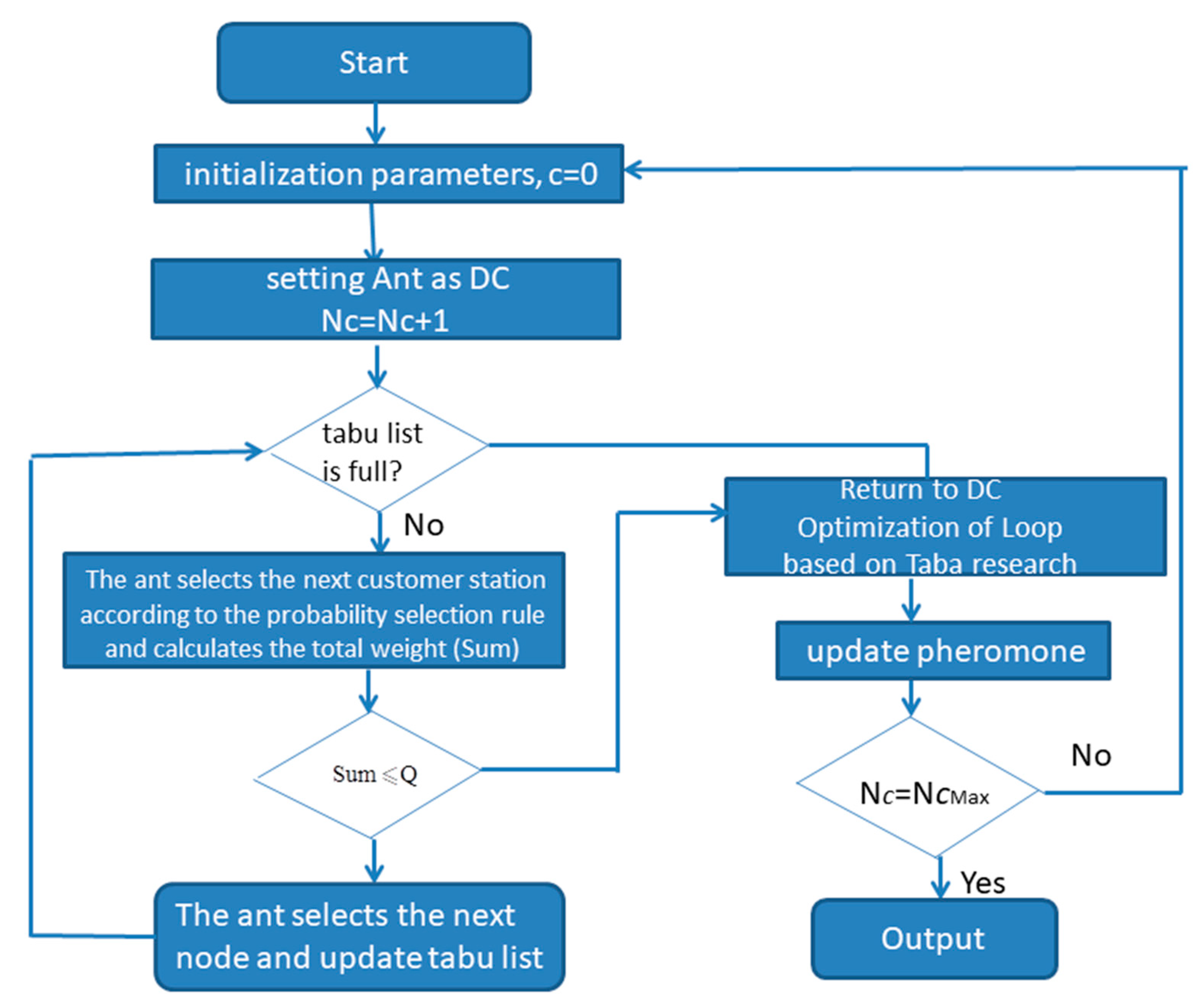
4.3. Calculation Steps of the Algorithm

According to the basic framework of the IACA and TS, the IACA is used to optimize the whole distribution path in global space. On the other hand, the TS is used to optimize the distribution path of a single vehicle in local space. The IACATS algorithm can be described as follows.
Step 1: Initialize. set the parameters of the Nc = 0, τ i j ( 0 ) = τ max , then carry out parameter initialization of τ i j k , α, β, ρ. The initial point should be included in the current disaggregation model and then be evaluated. The value of output is defined as Z;
Step 2: If the tabu list is not full, then improved ant colony algorithm is carried out. Except for the initial point, if it is not able to reach the vehicle quality time window required by vertex j in other remaining points, then it goes directly to the next step and calculate the total loading (Sum). On the contrary, if it is meet the requirements of vehicle quality and time window in the remaining points, it will select point j in a random manner to solve the transition probability Pkij parameter and combine this parameter with random number (0–1) for comparative analysis. If the requirements are met, transfer Ant k to Point j and place point j in the disaggregation model set. If the requirements are not met, the vertex needs to be selected again;
Step 3: when all points are in the disaggregation model set, solve zki. Then record the number of ants as m←k; otherwise, there is k←k+1, and then skip to step 2 and re-operate;
Step 4: if the Sum generated in step 2 is less than Q, select tabu local search mechanism to realize ant path optimization;
Step 5: solve the objective function value and updated pheromone. If Nc = Nc max, then end the iterations. If not, then turn back step 2 and reserve the current non-inferior solution;
Step 6: The next ant selects the different edges and update the tabu list. Given the edges (I,j) is the optimal path, it is analyzed to further solve τ i j (t+n) = ( 1 ρ ) τ i j ( t ) + Δ τ i j min ; given the edges (I,j) is the non-optimal path, it is analyzed to solve τ i j ( t + n ) = ( 1 ρ ) τ i j ( t ) ; finally, analyze all edges (I,j) and set Δ τ i j min 0, Nc Nc + 1 to update the tabu list;
Step 7: If the Nc parameter value is lower than the set number of iterations, go to step 2;
Step 8: If the Nc parameter value is lower than the set number of iterations, output to the optimal results.
Step 9: End. The above calculation process in schematic illustration is in Figure 2.

5. Case Study

Zhoushan Dayang Refrigerated Logistics Co., Ltd., which provides the distribution service of fresh agricultural products for 191 residential communities in Zhoushan Archipelago District, Zhejiang Province, was taken as the subject of the case study to collect distribution service data because of the short distance among the residential areas there. If separate distribution was carried out for each community, the distribution cost of the logistics company would be increased, and the efficiency would decrease. Therefore, this study took all residents’ committees as the distribution centers, and the k-means clustering method based on distance was adopted to aggregate the rest of the 87 communities into 20 distribution points. To convert these distribution points’ actual latitude and longitude coordinates to rectangular coordinates, they were set as the origin coordination. Then the daily demand for fresh agricultural products was estimated by calculating the number of permanent residents in the area served by each distribution point. The service time was the total service time of the residential areas covered by each distribution point. The basic information of the distribution centers and points is shown in Table 3.

Parameter Profile

In this paper, the 6.8 m refrigerated vehicle of brand name “Futian ruiwo” was selected as the cold chain distribution vehicle, of which the emission parameters are shown in Table 4.
Considering the actual situation of logistics operation, the price of fresh agricultural products was set at 4000 Yuan/t. The time window penalty coefficient was 0.0005, the vehicle speed was 50 km/h and its fixed cost was 500 Yuan per car every time. Moreover, the freshness degradation coefficient was 0.002. All customers ordered agricultural products with an acceptable freshness of 95%. In addition, the fuel CO2 emissions coefficient was 2.63 kg/L, the fuel price was 6.95 Yuan/L, the CO2 emissions price was 5 Yuan/kg and the biggest car load was 10 t.

6. Results

Based on above case study, related parameters of the improved genetic algorithm were set: the maximum number of iterations mg = 600. Using the MATLAB programming, the algorithm was run 20 times, and the result showed that the average total cost was 3625.68 Yuan, the average total time was 482.06 min and the average CO2 emissions was 44.48 kg. One of the most optimal distribution schemes is to use six transport vehicles to perform the distribution task with a total cost of 3602.73 Yuan. In addition, the total time spent was 477.33 min, and the total CO2 emissions was 43.02 kg. The specific distribution routing information is shown in Table 5. If the traditional method was employed, the distribution scheme would be as follows: eight transport vehicles would be used to complete the distribution task, and the total cost, total time and total CO2 emissions would be, respectively, 3840.55 Yuan, 505.12 min and 47.26 kg. In comparison, the improved genetic algorithm would reduce the dispatching of two refrigerated vehicles, cut the total cost by 4.94%, shorten the actual transportation distance by 5.50% and decrease the total CO2 emissions by 8.9%.

6.1. The Influences of Different Parameters on the Stability Performance of IACATS

In order to further investigate the influence of algorithm parameters on the model, we adjusted the values of α and β parameters here. The software Matlab 7.10.0 (R2010a) is used for programming and model solution analysis. The simulated results are shown in Table 6. Obviously, it can be seen that adjusting the values of α and β has no significant impact on the comprehensive cost. This suggests a good stability of IACATS.

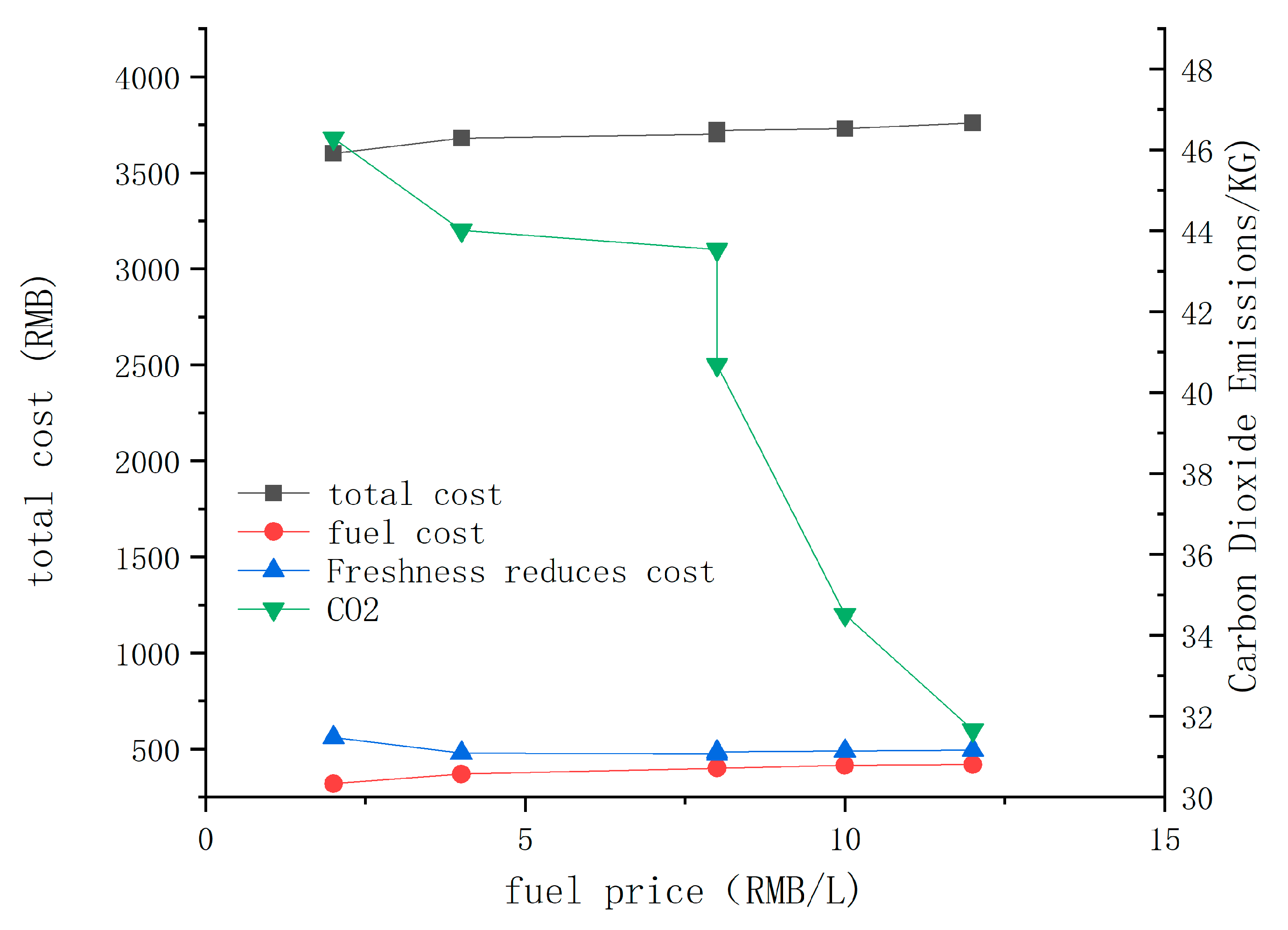
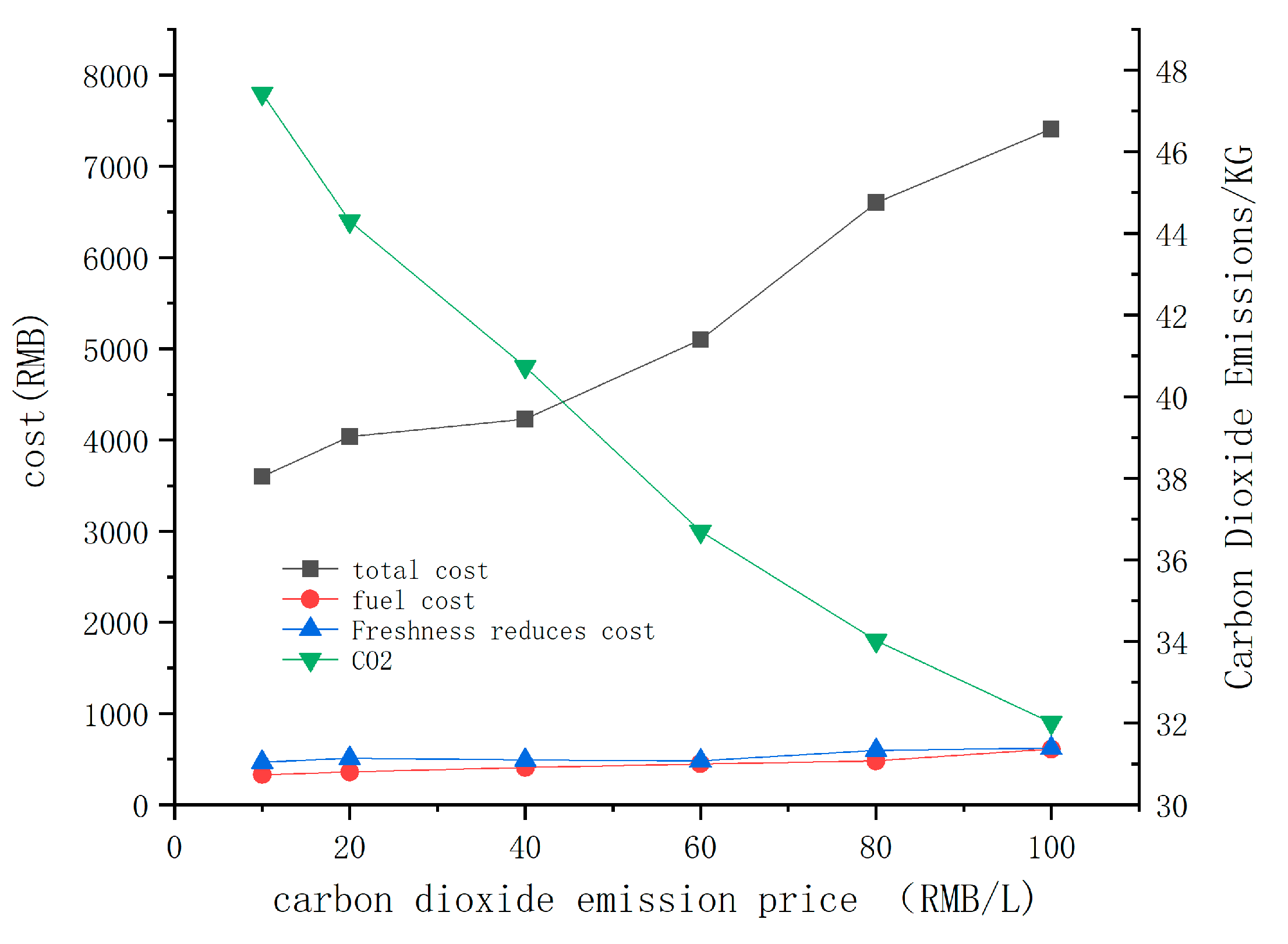
6.2. Parameter Sensitivity Analysis

In order to study the relationship of the change between the fuel price and CO2 emissions price and between carbon emissions and total cost in the optimization of cold chain distribution routing to fresh agricultural products, we adjusted different prices of fuel oil and CO2 emissions, as shown in Figure 3 and Figure 4.
It can be seen from Figure 3 that the total cost and fuel cost will rise with the increase of the fuel price. Meanwhile, the cost of freshness and CO2 emissions will decrease. Figure 4 shows that when the carbon price rises, the freshness degree will be decreased generally and the carbon emissions will decline. Therefore, in order to encourage the adoption of low carbon cold chain logistics distribution, it is necessary to appropriately raise the fuel price or carbon price. It not only can reduce CO2 emissions and energy consumption, but also decrease enterprises’ total costs. These experimental results would offer useful information to the government when figuring out corresponding policies and regulations. Moreover, these simulated results would serve as a reference for the selection of vehicle routing optimization of low carbon cold chain logistics.

6.3. Effectiveness Analysis of IACATS Algorithm

In order to demonstrate the feasibility and superiority in the proposed algorithm, we compared it with the other heuristic algorithm. The evolution process is shown in Figure 5. It can be seen from Figure 5 that in the early operation stage of the algorithm, the cost objective function value of the improved algorithm is smaller than that of the standard ant colony algorithm. However, in the process of evolution, the convergence rate of the former is faster than that of the latter, which indicates that the introduction of the TS can help to increase the “hybrid computing power” of the algorithm and promote the convergence rate. Moreover, the optimization result of the improved algorithm is closer to the global optimal, with a cost objective function value of 3650.79. It is obviously better than that of the standard colony algorithm (3840.55).
In order to demonstrate the superiority of this method, intelligent algorithm (this work), Multiple Ant Colony Optimization Algorithm (MACOA) [65] and Non-dominated Sorting Genetic Algorithm (NSGA) [66] are selected in this paper to solve the problem respectively. We assumed the number of iterations as 100 times. The final result is as follows (Table 7).
By comparing the data in Table 3, it can be found that the IACATS algorithm proposed in this paper is better than NSGA and MACOA for solving the optimization problem of cold chain logistics distribution path considering the parameters of research time, search success rate or average iteration of number. Moreover, the proposed algorithm in this paper has great advantages over genetic algorithm and ant colony algorithm. For instance, average iteration of number decreases from 48 to 16.

7. Discussion

In the last two decades, the popular issues of greenhouse gas emissions reduction and the difficulty in preserving the nutritional characteristics of fresh food-stuffs during cold chain logistics have attracted attention among the world. The above two issues are mainly involved in VRP. VRP is a vital problem and a crucial link in reducing the total cost of distribution of cold chain logistics. We used novel IACATS algorithm and MATLAB programming to solve LCFD-VRP model. Our results demonstrate that IACATS could reduce the dispatching of two refrigerated vehicles, thus lowering the total cost by 4.94%, shortening the real transportation distance by 5.50% and cutting the total CO2 emissions by 8.9% compared with the traditional ant algorithm mode. Therefore, the LCFD-VRP model we proposed can effectively help to achieve the low carbon emissions and low cost of fresh agricultural products. This suggests that the proposed model and IACATS algorithm would be used to design and operate food distribution systems with high-quality fresh food and less environmental pollution.
The VRP and its variants have been studied in many previous works [67,68,69,70]. However, few studies have considered routing optimization based on CO2 emissions and fresh food. In addition, the influence of the energy consumption of refrigeration equipment on carbon emissions is often ignored. This paper aims to deal with optimization of VRP with CO2 emission and fresh food. Most of the models only considered CO2 emissions from the generation of fuel consumption [49]. CO2 emissions in this paper are derived from two parts: the generation of fuel consumption and the energy consumption of refrigeration equipment. In order to achieve the lowest cost as the objective function, we considered costs such as the fixed costs, carbon emissions cost, time window penalty cost and freshness penalty cost. These costs cover most of the costs in cold chain logistics. Even though we considered the above-mentioned cost factors in the proposed model, more cost factors, such as fresh food damage costs, fresh food shortage costs and waiting time costs, should be included in the future model from the perspective overall consideration.
Since VRP is a typical NP-hard problem. The exact algorithm is rather important to successfully solve the VRP. In this paper, we employed the improved ant colony algorithm and the TS algorithm to solve LCFD-VRP model. The results of effectiveness and sensitivity indicated that combination of two algorithms exerted excellent effect based on the advantage of improved ant colony algorithm in global search and TS in local optimization ability. Compared with MACOA and NSGA methods, the results including research success rate and average number of iterations in our study are obviously better than of MACOA or NSGA. It is suggested that the combination of other various exact methods, approximation algorithms and heuristic algorithms is a useful method to solve VRP. Total CO2 emissions reduced by 8.9% in our study shows that LCFD-VRP model can effectively reduce carbon emissions. From the government’s consideration, this method could be promoted in other similar cold chain logistics to raise the awareness of low carbon logistics. On the other hand, from cold chain logistics enterprise’s consideration, this method should be introduced into the daily routing optimization of cold chain logistics, because it can reduce the operation cost and can fulfill enterprise’s social responsibility, which inversely improve the competitiveness of enterprises in the marketplace.
Aiming at optimization of vehicle routing problem in cold chain logistics to fresh agricultural products, we used the routing data from Zhoushan Dayang Refrigerated Logistics Co., Ltd. as the practical sample. Normally, researchers have carried out multiple deposit distribution centers as the collect distribution service [71,72]. In this study, we employed one distribution center and another twenty distribution points as the collect distribution service because of small area of the selected sample. If we used more distribution centers, it would reduce the accuracy of the proposed model. Hence, depending on the kind of model we employed, we need to use the model according to the local environment to adjust it. This is another attractive topic to be carried out in the future, for instance, the area, population density and income level, etc.
In this study, we obtained the overall optimization of cold chain logistics through different settings for parameter values. However, due to experimental limitations, extensive and comprehensive comparative experiments will need to be applied to the LCFD-VRP model to get better overall optimization results in future research. Even though it achieved good stimulation results, how to adjust the parameters of the algorithm and how to optimize the structure of the algorithm while ensuring higher accuracy were not considered in the constructed model or proposed algorithm. Especially the uncertainty of customers’ demands (or satisfaction) was not considered in the LCFD-VRP model based on the background of a low-carbon economy. Furthermore, there will be a more complex environment in the real operation of routing problem. In addition, traffic jam situations can be employed in the distribution routing planning as the introduction of a road congestion index into the model will be better able to reflect the real feasible solution. Hence, further research is required to consider more factors in order to be more adaptable to real-life scenarios.

8. Conclusions

In this paper, the optimization of cold chain logistics routing problem was studies while we considered carbon emissions and product freshness. IACATS algorithm was proposed to effectively solve the LCDF-VRP model. According to the example, the effectiveness and applicability of the LCFD-VRP model was verified. Through the simulation value, it can be seen that the results of the optimization compared with the traditional algorithm reduce the CO2 emissions and raise the food fresh degree. The experimental results of this paper provide management suggestions for logistics enterprises to effectively balance economic costs and environmental costs in vehicle routing problems.
The main conclusions are listed as follows:
(1) In view of the particularity in the cold chain logistics of perishable products, and the requirement of low carbon green logistics, the fixed cost, fuel cost, time window penalty cost, freshness degradation punishment and the cost of carbon emissions can minimize the total costs in the logistics distribution vehicle route optimization model. The model considering above factors seems to be more reasonable, which is similar to the real demand.
(2) Since the vehicle routing problem of logistics distribution is a typical NP problem, IACA algorithm based on the TS has been successfully designed to solve the LCDF-VRP model. IACATS could reduce two refrigerated vehicles, decrease the total cost by 4.94%, shorten the actual transportation distance by 5.50%, and cut down the total CO2 emissions by 8.9%. Therefore, the LCFD-VRP model can effectively help cold chain logistics enterprises to reduce the low carbon emissions and increase high quality fresh agricultural products.
(3) The case study shows that the optimization model and solving algorithm of cold chain logistics routing problem are effective at reducing carbon emissions and ensuring the freshness of products. It not only provides scientific theoretical guidance to cold chain logistics companies for further optimization of daily distribution routing, but also helps in solving the practical problems of agricultural products in the cold chain delivery. This method can also be helpful to the government to carry out incentive policies, and simultaneously promotes enterprises to exert their social responsibility and establish good impression to the public.

Author Contributions

Conceptualization, J.C.; formal analysis, J.C. and Y.Z.; methodology, J.C.; project administration, S.N.; resources, J.C. software, T.D. and P.G.; supervision, Y.Z., S.N.; writing—original draft, J.C.; writing—review and editing, S.N. and J.C.

Funding

YT.Z acknowledges funding from Zhoushan Science and Technology project (2018C21010) and start-up Research Funding from Zhejiang Ocean Uiversity (12215090117). J.C acknowledges funding from Zhoushan Free Trade Zone.

Acknowledgments

This paper was supported by Wonkwang University in 2019 and Project from Zhoushan Free Trade Zone in Zhejiang Province.

Conflicts of Interest

The authors declare no conflict of interest.

References

  1. Montanari, R. Cold chain tracking: A managerial perspective. Trends Food Sci. Technol. 2008, 19, 425–431. [Google Scholar] [CrossRef]
  2. Fan, J.; Li, J.; Wu, Y.; Wang, S.; Zhao, D. The effects of allowance price on energy demand under a personal carbon trading scheme. Appl. Energy 2016, 170, 242–249. [Google Scholar] [CrossRef]
  3. Wang, K.; Zhang, X.; Wei, Y.-M.; Yu, S. Regional allocation of CO2 emissions allowance over provinces in China by 2020. Energy Policy 2013, 54, 214–229. [Google Scholar] [CrossRef]
  4. Verbič, M. Discussing the parameters of preservation of perishable goods in a cold logistic chain model. Appl. Econ. 2006, 38, 137–147. [Google Scholar] [CrossRef]
  5. Ho, W.; Ang, J.; Lim, A. A hybrid search algorithm for the vehicle routing problem with time windows. Int. J. Artif. Intell. Tools 2001, 10, 431–449. [Google Scholar] [CrossRef]
  6. Wang, S.; Tao, F.; Shi, Y.; Wen, H. Optimization of Vehicle Routing Problem with Time Windows for Cold Chain Logistics Based on Carbon Tax. Sustainability 2017, 9, 694. [Google Scholar] [CrossRef]
  7. Chameides, W.; Oppenheimer, M. Carbon trading over taxes. Science 2007, 315, 1670. [Google Scholar] [CrossRef]
  8. Maden, W.; Eglese, R.W.; Black, D. Vehicle routing and scheduling with time-varying data: A case study. J. Oper. Res. Soc. 2010, 61, 515–522. [Google Scholar] [CrossRef]
  9. Iv, J.H.W.; Cavalier, T.M. A Genetic Algorithm for the Split Delivery Vehicle Routing Problem. Am. J. Oper. Res. 2012, 2, 207–216. [Google Scholar]
  10. Archetti, C.; Bianchessi, N.; Speranza, M.G. Branch-and-cut algorithms for the split delivery vehicle routing problem. Eur. J. Oper. Res. 2014, 238, 685–698. [Google Scholar] [CrossRef]
  11. Dror, M.; Trudeau, P. Savings by split delivery routing. Transp. Sci. 1989, 23, 141–145. [Google Scholar] [CrossRef]
  12. Thongwan, T.; Kangrang, A.; Prasanchum, H. Multi-objective future rule curves using conditional TS algorithm and conditional genetic algorithm for reservoir operation. Heliyon 2019, 5, e02401. [Google Scholar] [CrossRef] [PubMed]
  13. Berbotto, L.; Garcia, S.; Nogales, F. A randomized granular TS heuristic for the split delivery vehicle routing problem. Ann. Oper. Res. 2014, 222, 153–173. [Google Scholar] [CrossRef]
  14. Ho, S.; Haugland, D. A TS heuristic for the vehicle routing problem with time windows and split deliveries. Comput. Oper. Res. 2004, 31, 1947–1964. [Google Scholar] [CrossRef]
  15. Hsiao, Y.; Chen, M.; Chin, C. Distribution planning for perishable foods in cold chains with quality concerns: Formulation and solution procedure. Trends Food Sci. Technol. 2016, 61, 80–93. [Google Scholar] [CrossRef]
  16. Cheng, R.; Gen, M. Fuzzy vehicle routing and scheduling problem using genetic algorithm. In Genetic Algorithms and Soft Computing; Herrera, F., Verdegay, J., Eds.; Springer: Berlin, Germany, 1996; pp. 683–709. [Google Scholar]
  17. Zhang, J.; Wang, W.; Zhao, Y.; Cattani, C. Multiobjective Quantum Evolutionary Algorithm for the Vehicle Routing Problem with Customer Satisfaction. Math. Probl. Eng. 2012, 2012, 1–19. [Google Scholar] [CrossRef]
  18. Comodi, G.; Renzi, M.; Rossi, M. Energy efficiency improvement in oil refineries through flare gas recovery technique to meet the emission trading targets. Energy 2016, 109, 1–12. [Google Scholar] [CrossRef]
  19. Hsu, C.-I.; Hung, S.-F.; Li, H.-C. Vehicle routing problem with time-windows for perishable food delivery. J. Food Eng. 2007, 80, 465–475. [Google Scholar] [CrossRef]
  20. Amorim, P.; Parragh, S. A rich vehicle routing problem dealing with perishable food: A case study. Top 2014, 22, 489–508. [Google Scholar] [CrossRef]
  21. Lai, M.; Cao, E. An improved differential evolution algorithm for vehicle routing problem with simultaneous pickups and deliveries and time windows. Eng. Appl. Artif. Intell. 2010, 23, 188–195. [Google Scholar]
  22. Anderson, E.W.; Sullivan, M.W. The Antecedents and Consequences of Customer Satisfaction for Firms. Mark. Sci. 1993, 12, 125–143. [Google Scholar] [CrossRef]
  23. Chung, L.M.; Wirtz, J. Book Review: Satisfaction: A Behavioral Perspective on the Consumer. Asia Pac. J. Manag. 1998, 15, 285–286. [Google Scholar] [CrossRef]
  24. Qin, Q.; Liu, Y.; Li, X.; Li, H. A multi-criteria decision analysis model for carbon emission quota allocation in China’s east coastal areas: Efficiency and equity. J. Clean. Prod. 2017, 168, 410–419. [Google Scholar] [CrossRef]
  25. Wang, X. Changes in CO2 Emissions Induced by Agricultural Inputs in China over 1991–2014. Sustainability 2016, 8, 414. [Google Scholar] [CrossRef]
  26. Yi, W.-J.; Zou, L.-L.; Guo, J.; Wang, K.; Wei, Y.-M. How can China reach its CO2 intensity reduction targets by 2020? A regional allocation based on equity and development. Energy Policy 2011, 39, 2407–2415. [Google Scholar] [CrossRef]
  27. Drezner, Z.; Scott, C.H. Location of a distribution center for a perishable product. Math. Methods Oper. Res. 2013, 78, 301–314. [Google Scholar] [CrossRef]
  28. GhannadPour, S.F.; Noori, S.; Tavakkoli-Moghaddam, R. Multiobjective Dynamic Vehicle Routing Problem with Fuzzy Travel Times and Customers’ Satisfaction in Supply Chain Management. IEEE Trans. Eng. Manag. 2013, 60, 777–790. [Google Scholar] [CrossRef]
  29. Wang, S.; Tao, F.; Shi, Y. Optimization of Inventory Routing Problem in Refined Oil Logistics with the Perspective of Carbon Tax. Energies 2018, 11, 1437. [Google Scholar] [CrossRef]
  30. Shen, L.; Tao, F.; Wang, S. Multi-Depot Incomplete Open Vehicle Routing Problem with Time Windows Based on Carbon Trading. Int. J. Environ. Res. Public Health 2018, 15, 2025. [Google Scholar] [CrossRef]
  31. Niu, Y.; Yang, Z.; Chen, P.; Xiao, J. Optimizing the green open vehicle routing problem with time windows by minimizing comprehensive routing cost. J. Clean. Prod. 2017, 171, 962–971. [Google Scholar] [CrossRef]
  32. Guo, J.; Liu, C. Time-Dependent Vehicle Routing of Free Pickup and Delivery Service in Flight Ticket Sales Companies Based on Carbon Emissions. J. Adv. Transp. 2017, 2017, 1–14. [Google Scholar] [CrossRef]
  33. Naderipour, M.; Alinaghian, M. Measurement, evaluation and minimization of CO2, NOx, and CO emissions in the open time dependent vehicle routing problem. Measurement 2016, 90, 443–452. [Google Scholar] [CrossRef]
  34. Liao, T. On-Line Vehicle Routing Problems for Carbon Emissions Reduction. Comput. Civ. Infrastruct. Eng. 2017, 32, 1047–1063. [Google Scholar] [CrossRef]
  35. Liu, J. A national customer satisfaction barometer: The Swedish experience. J. Mark. 1992, 56, 6–21. [Google Scholar]
  36. Fornell, C.; Johnson, M.D.; Anderson, E.W.; Cha, J.; Bryant, B.E. The American Customer Satisfaction Index: Nature, Purpose, and Findings. J. Mark. 1996, 60, 7. [Google Scholar] [CrossRef]
  37. Zeng, Z.; Jiang, Z.; Xu, X. Research on the performance evaluation model of logistic company’s distribution. Ind. Eng. Manag. 2003, 3, 40–44. [Google Scholar]
  38. Parasuraman, A.; Zeithaml, V.A.; Berry, L.L. A Conceptual Model of Service Quality and Its Implications for Future Research. J. Mark. 1985, 49, 41. [Google Scholar] [CrossRef]
  39. Wang, S.; Tao, F.; Shi, Y. Optimization of Location–Routing Problem for Cold Chain Logistics Considering Carbon Footprint. Int. J. Environ. Res. Public Health 2018, 15, 86. [Google Scholar] [CrossRef] [Green Version]
  40. Bao, C.; Zhang, S. Route optimization of cold chain logistics in joint distribution: With consideration of carbon emission. Ind. Eng. Manag. 2018, 23, 95–107. [Google Scholar]
  41. Gao, J.; Yuan, Z.; Liu, X.; Xia, X.; Huang, X.; Dong, Z. Improving air pollution control policy in China—A perspective based on cost-benefit analysis. Sci. Total. Environ. 2016, 543, 307–314. [Google Scholar] [CrossRef]
  42. Lin, W.; Ma, Z.; Tsay, M. An improved TS for economic dispatch with multiple minima. Power Eng. Rev. IEEE 2002, 22, 70. [Google Scholar] [CrossRef]
  43. Zheng, G.; Liu, L.; Deng, L. Location-Routing Optimization of Cold Chain Distribution Center Based on Hybrid Genetic Algorithm-TS. In Proceedings of the 14th COTA International Conference of Transportation Professionals, Changsha, China, 4–7 July 2014. [Google Scholar]
  44. Shi, Z.; Zhuo, F. Distribution location routing optimization problem of food cold chain with time window in time varying network. Appl. Res. Comput. 2013, 30, 183–188. [Google Scholar]
  45. Karaoglan, I.; Altiparmak, F.; Kara, I.; Dengiz, B. A branch and cut algorithm for the location-routing problem with simultaneous pickup and delivery. Eur. J. Oper. Res. 2011, 211, 318–332. [Google Scholar] [CrossRef]
  46. Afshar, A.; Haghani, A. Modeling integrated supply chain logistics in real-time large-scale disaster relief operations. Socio-Econ. Plan. Sci. 2012, 46, 327–338. [Google Scholar] [CrossRef]
  47. Li, J.; Zhang, J. Study on the effect of carbon emission trading mechanism on logistics distribution routing decisions. Syst. Eng. Theory Pract. 2014, 34, 1779–1787. [Google Scholar]
  48. Guo, H.; Ming, S. Process reengineering of cold chain logistics of agricultural products based on low-carbon economy. Asian Agric. Res. 2012, 5, 59–62. [Google Scholar]
  49. Meneghetti, A.; Monti, L. Greening the food supply chain: An optimisation model for sustainable design of refrigerated automated warehouses. Int. J. Prod. Res. 2015, 53, 6567–6587. [Google Scholar] [CrossRef]
  50. Xiao, Y.; Zhao, Q.; Kaku, I.; Xu, Y. Development of a fuel consumption optimization model for the capacitated vehicle routing problem. Comput. Oper. Res. 2012, 39, 1419–1431. [Google Scholar] [CrossRef]
  51. Ji, Y. Decision Optimization for Cold Chain Logistics of Fresh Agricultural Products under the Perspective of Cost-Benefit. Open Access Libr. J. 2019, 6, 1–17. [Google Scholar] [CrossRef]
  52. You, H.; Wang, X. Interactive genetic algorithm based on tournament selection and its application. J. Chin. Comput. Syst. 2009, 30, 1824–1827. [Google Scholar]
  53. Brandão, J. A TS algorithm for the open vehicle routing problem. Eur. J. Oper. Res. 2004, 157, 552–564. [Google Scholar] [CrossRef]
  54. Fan, J. The Vehicle Routing Problem with Simultaneous Pickup and Delivery Based on Customer Satisfaction. Procedia Eng. 2011, 15, 5284–5289. [Google Scholar] [CrossRef] [Green Version]
  55. Cheng, R.; Gen, M.; Tozawa, T. Vehicle Routing Problem with Fuzzy Due-time Using Genetic Algorithms. J. Jpn. Soc. Fuzzy Theory Syst. 1995, 7, 1050–1061. [Google Scholar] [CrossRef] [Green Version]
  56. Afshar-Bakeshloo, M.; Mehrabi, A.; Safari, H.; Maleki, M.; Jolai, F. A green vehicle routing problem with customer satisfaction criteria. J. Ind. Eng. Int. 2016, 12, 529–544. [Google Scholar] [CrossRef] [Green Version]
  57. Xia, Y.; Fu, Z. A TS algorithm for distribution network optimization with discrete split deliveries and soft time windows. Clust. Comput. 2018, 18, 586–597. [Google Scholar]
  58. Masson, R.; Røpke, S.; Lehuédé, F.; Péton, O. A branch-and-cut-and-price approach for the pickup and delivery problem with shuttle routes. Eur. J. Oper. Res. 2014, 236, 849–862. [Google Scholar] [CrossRef]
  59. Colorni, A.; Dorigo, M.; Maniezzo, V. Distributed optimization by ant colonies. In Proceedings of the European Conference on Artificial Life, ECAL’91, Paris, France, 11–13 December 1991; pp. 134–142. [Google Scholar]
  60. Osvald, A.; Stirn, L.Z. A vehicle routing algorithm for the distribution of fresh vegetables and similar perishable food. J. Food Eng. 2008, 85, 285–295. [Google Scholar] [CrossRef]
  61. Bogataj, M.; Bogataj, L.; Vodopivec, R. Stability of perishable goods in cold logistic chains. Int. J. Prod. Econ. 2005, 93, 345–356. [Google Scholar] [CrossRef]
  62. Chen, H.-K.; Hsueh, C.-F.; Chang, M.-S. Production scheduling and vehicle routing with time windows for perishable food products. Comput. Oper. Res. 2009, 36, 2311–2319. [Google Scholar] [CrossRef]
  63. Boventer, E.V. The relationship between transportation costs and location rent in transportation problems. J. Reg. Sci. 2010, 3, 27–40. [Google Scholar] [CrossRef]
  64. Solomon, M.M. Algorithms for the Vehicle Routing and Scheduling Problems with Time Window Constraints. Oper. Res. 1987, 35, 254–265. [Google Scholar] [CrossRef] [Green Version]
  65. Shen, L.; Tao, F.; Shi, Y.; Qin, R. Optimization of Location-Routing Problem in Emergency Logistics Considering Carbon Emissions. Int. J. Environ. Res. Public Health 2019, 16, 2982. [Google Scholar] [CrossRef] [Green Version]
  66. Liu, C.; Kou, G.; Peng, Y.; Alsaadi, F.E. Location-Routing Problem for Relief Distribution in the Early Post-Earthquake Stage from the Perspective of Fairness. Sustainability 2019, 11, 3420. [Google Scholar] [CrossRef] [Green Version]
  67. Rath, S.; Gutjahr, W.J. A math-heuristic for the warehouse location–routing problem in disaster relief. Comput. Oper. Res. 2014, 42, 25–39. [Google Scholar] [CrossRef]
  68. Prins, C.; Prodhon, C.; Ruiz, A.; Soriano, P.; Calvo, R.W. Solving the Capacitated Location-Routing Problem by a Cooperative Lagrangean Relaxation-Granular Tabu Search Heuristic. Transp. Sci. 2007, 41, 470–483. [Google Scholar] [CrossRef]
  69. Cooper, L. The Transportation-Location Problem. Oper. Res. 1972, 20, 94–108. [Google Scholar] [CrossRef] [Green Version]
  70. Zhao, Y.; Fan, J.; Liang, B.; Zhang, L. Evaluation of Sustainable Livelihoods in the Context of Disaster Vulnerability: A Case Study of Shenzha County in Tibet, China. Sustainability 2019, 11, 2874. [Google Scholar] [CrossRef] [Green Version]
  71. Ting, J.; Chen, H. A multiple ant colony optimization algorithm for the capacitated location routing problem. Int. J. Prod. Econ. 2013, 141, 34–44. [Google Scholar] [CrossRef]
  72. Toro, E.M.; Franco, J.F.; Echeverri, M.G.; Guimarães, F.G. A multi-objective model for the green capacitated location-routing problem considering environmental impact. Comput. Ind. Eng. 2017, 110, 114–125. [Google Scholar] [CrossRef] [Green Version]
Figure 1. Flowchart of this study.
Sustainability 11 06584 g001
Figure 2. Flowchart of the improved genetic algorithm.
Sustainability 11 06584 g002
Figure 3. The relationship between fuel price, total cost and carbon emissions.
Sustainability 11 06584 g003
Figure 4. The relationship between CO2 emissions price, total cost and carbon emissions.
Sustainability 11 06584 g004
Figure 5. Comparison of evolution process between standard and improved ant colony algorithm.
Sustainability 11 06584 g005
Table 1. Symbols and descriptions in the model.
Symbols Descriptions
x i j k 0–1 are decision variables. If k car serves customer point i, and goes to serve customer point j, x i j k = 1, otherwise x i j k = 0.
dijThe distance from customer point i to customer point j/km
P1The price of fresh agricultural products transported/(RMB t−1)
P2The price of fuel used by distribution vehicles/(RMB L−1)
P3Real-time carbon trading prices on the carbon exchange/(RMB t−1)
P4Fixed cost of the delivery vehicle/(RMB car number−1)
SiService time/min of the delivery vehicle at customer point i
[ i , l i , l ¯ i ] Time window requirements of customer point i. Particularly, [ i , l i ] is the best receiving time for customers, and l ¯ i is the latest receiving time that customers can tolerate.
K ¯ Distribution vehicle collection K ¯ = {1,2,3, ⋯,Κ}, where K represents the maximum number of vehicles in the distribution center
QMaximum load of the distribution vehicle/t
qiQuantity demanded/t at customer point i
ρCO2 emissions index
FiRequirement of customers order i on fresh agricultural products
v0Delivery vehicle speed/(km h−1)
The freshness decreasing coefficient of produce
θTime window penalty coefficient
Table 2. Parameters and descriptions about the fuel and carbon cost.
Parameter Description
ξFuel to air mass ratio
κCalorific value of the fuel engine/(kJ g−1)
ψConversion coefficient/(from g s-1 to L s−1)
bEngine friction coefficient
MEngine speed
ωWithout loading in the vehicle/kg
gAcceleration of gravity
εRoad slope
CrRolling resistance coefficient
vVehicle speed
CdAir resistance coefficient
ntfVehicle transmission efficiency
ηFuel engine efficiency parameters
τVehicle acceleration
U j k Load when vehicle k reaches customer point j
PAir density/(kg m−3)
VEngine capacity/VL
SFrontal surface area
Table 3. Basic information of distribution centers and points.
No.Horizontal Axis/mVertical Axis/mFixed Time WindowAcceptable Time WindowQuantity Demanded/tService Time/min
0005:30–17:005:00–17:0000
1−189.24556:00–7:006:00–7:300.815
2103.814526:20–7:306:20–8:003.3519
31103.54266:00–6:506:00–7:202.9517
41264.712897:00–8:007:00–8:202.411
51221.2−18426:40–7:306:40–8:002.7514
61436.6−20256:00–7:006:00–7:403.320
7245.6−6726:30–7:006:30–7:302.815
82350.0−11896:20–7:306:20–8:003.2510
91148.7−4256:00–7:306:00–8:302.1515
101025.2−276:20–8:006:20–9:003.0518
11863.6−12146:20–7:406:20–8:003.216
121785.6−9577:30–8:507:30–9:203.511
13682.4−33566:00–7:306:00–8:000.5515
14134.6−28796:40–7:506:40–8:302.719
15−485.4−16896:20–7:006:20–8:001.714
16423.1−21966:00–7:006:00–7:302.2510
17444.3−9836:00–6:406:00–7:102.7515
181168.7−17867:00–8:007:00–9:001.920
19−568.3−6226:00–6:506:00–7:203.1514
20−722.4−20896:50–7:306:50–8:10111
Table 4. Emission parameters of the 6.8 m refrigerated vehicle.
Parameter Implication Value
ωVehicle weight/kg6350
ξFuel-to-air-mass ratio1
bEngine friction coefficient0.2
MEngine speed33
VEngine capacity/L5
gAcceleration of gravity 9.81
CrRolling resistance coefficient0.01
ηFuel engine efficiency parameters0.9
κCalorific value of fuel engine/(kJ·g−1)44
ψConversion coefficient737
ntfVehicle transmission efficiency0.4
CdCoefficient of air resistance0.7
PAir density/(kg m−3)1.2041
SFrontal surface are/m23.912
Table 5. Optimization results of vehicle distribution routing.
Number of Vehicles Distribution Routing Cost/RMBLoading Rate/%CO2 Emissions/kgTotal Time/min
10-19-2-8-0528.2296.879.2363.78
20-17-15-14-0534.2572.525.0166.89
30-1-10-6-20-0658.7283.208.9683.56
40-16-11-4-0632.0279.687.2574.25
50-13-5-12-0589.3668.797.95105.23
60-9-3-7-18-0657.8599.037.0283.87
Table 6. Adjust α and β parameters and simulated results.
(α,β)KZ
(1,1)43587
(1,2)33581
(1,3)33576
(2,1)33590
(2,2)33586
(2,3)33598
Table 7. Compared results to other well-known methods.
TypeResearch Time/sSearch Success Rate/%Average Numberof Iterations
NSGA2 722.67648
MACOA2 692.88530
this work2534.39816

