Maintenance Cost Estimation in PSCI Girder Bridges Using Updating Probabilistic Deterioration Model

Abstract

A deterioration model plays an important role to predict the valid total maintenance cost for sustainable maintenance of bridges. In the current state-of-the-art, the deterioration model has regression parameters as a probabilistic process by an initially determined mean and standard deviation, called an existing model. However, the existing model has difficulty to predict maintenance costs accurately, because it cannot reflect an information based on structural damage at an operational stage. In this research, updating the probabilistic deterioration model is presented for the prediction of pre-stressed concrete I-type (PSCI) girder bridges using a particle filtering technique which is an advanced Bayesian updating method based on big data analysis. The method enables predicting maintenance cost fitted in the current structural status, which includes the recent information by inspection with bridge-monitoring. The method is adapted in the Mokdo Bridge which is currently being used for evaluating the efficiency of maintenance cost by effects on updated probabilistic values with two different scenarios. As the result, it is shown that the proposed method is effective in predicting maintenance costs.

1. Introduction

An accurate the deterioration prediction of the existing bridge is very important for sustainable maintenance. Maintaining bridges with optimal maintenance activities by forecasting bridge performance with periodical inspection data is an interesting issue. These days, the bridge deterioration model based on regression analysis is conducted to derive an efficient maintenance method for bridge management system in advanced countries, such as the USA, Japan, and Australia [1,2,3]. Domestic and foreign research trends related to bridge maintenance denote that they have focused on estimating the bridge performance changes with high accuracy through monitoring technologies based on unmanned inspection devices (sensors, drones, or robots) and by establishing an optimal maintenance decision making process system [4,5,6,7,8,9,10,11,12,13,14,15]. In addition, Bayesian deterioration model updating for maintenance cost estimation in steel box girder bridges has been proposed [16]. However, these studies are insufficient to predict maintenance costs accurately.

In this paper, a new preventive bridge maintenance method is proposed using the monitoring technologies that can be applied to determine the condition of the bridge by the early detection of damages during the actual use of bridges with high accuracy. First, a deterioration model has been developed by each bridge member based on the bridge’s aging characteristics. Second, we have considered a particle filtering technique based on the Bayesian approach with which the performance changes of the target bridge that is in use can be accurately predicted by incorporating the monitoring information into the probability characteristic values of the deterioration model (the mean and standard deviation). Third, we presented a maintenance cost analysis model by linking the repair and reinforcement method application probability with the repair and reinforcement method cost model using the rating of the target bridge. Additionally, we determined the economic effect in terms of the lifecycle cost efficiency of the deterioration model-based preventive maintenance scenario, which was renewed by the particle filtering technique, when compared to the existing maintenance scenario of the target bridge that is currently in use. Figure 1 shows a detailed development process of the proposed method for preventive management by eight steps.

2. Bridge Deterioration Model

The bridge deterioration model can be developed by the deterministic model. The deterministic model by regression analysis based on inspection data is considering many elements exerting an influence on the bridge deterioration, and it is efficient to develop the deterioration model by bridge or span. However, the uncertainty of bridge deterioration is difficult to consider. As to the stochastic model, there is the advantage of considering the uncertainty of the deterioration process. Therefore, the statistic value (standard deviation) is used to consider the uncertainty.

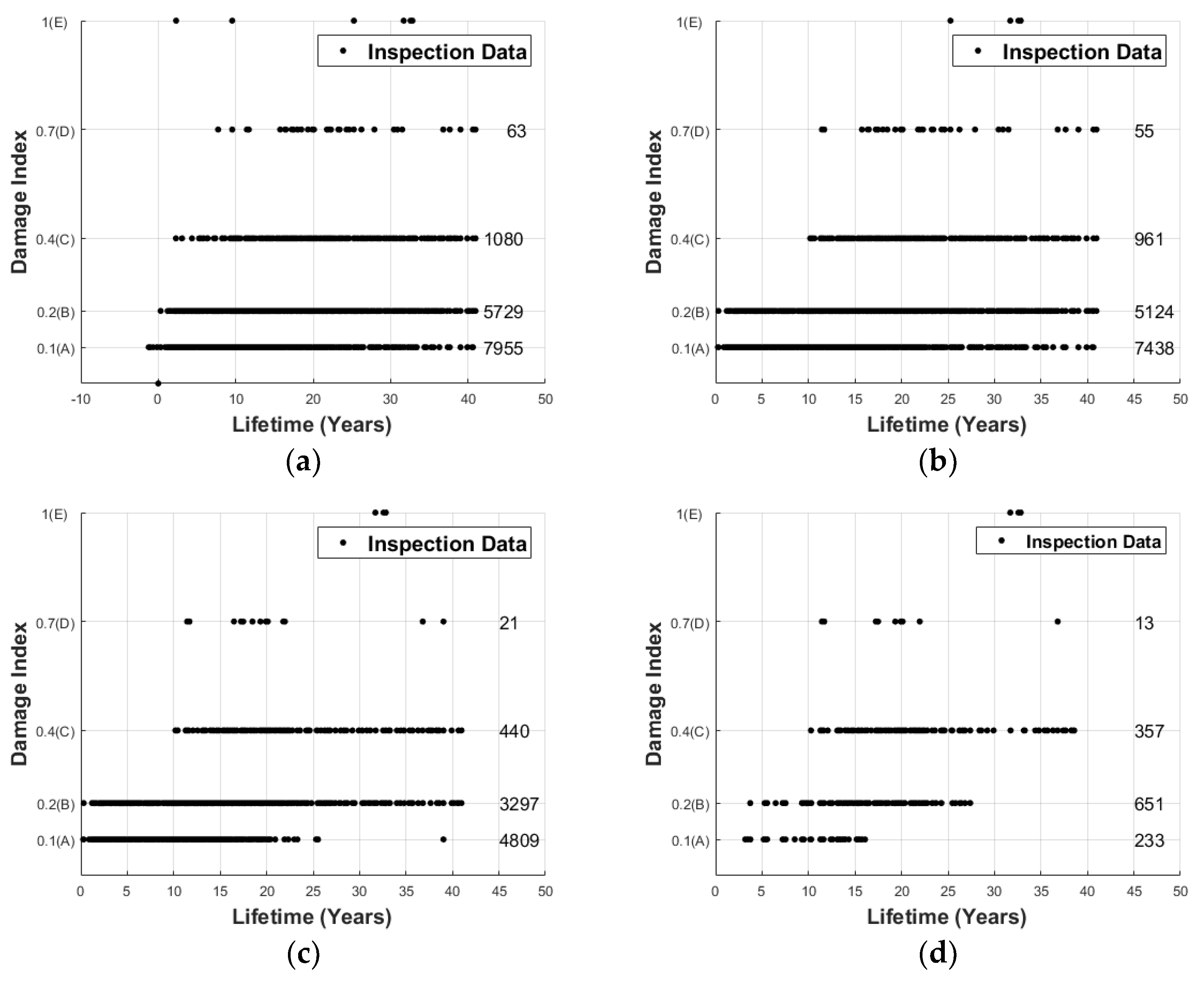
2.1. Cleansing Data for Prediction of Bridge Deterioration

The inspection data used in this paper is the condition rating data from domestic national highway bridges. The inspection types of condition ratings are largely divided into regular inspection (monthly and half-yearly), precise inspection, precise safety diagnosis, and emergency inspection. The condition rating databases of precise inspection and precise safety diagnosis were used in this study as the reliability of these databases is higher than that of other types of conditions rating databases when the inspection procedures are taken into account. As precise safety diagnosis began from 1995, the inspection data dated after 1995 was used. As a model for the condition change after completion of the construction should be generated because a condition deterioration model without any improvement action is to be developed, the condition rating data of the bridges completed after 1990 were used (the scope of the rating history data collection of Type 1 and Type 2 national highway bridges obtained from the bridge management system (BMS) of the Korea Institute of Civil Engineering and Building Technology (KICT): 1995–2018). Moreover, a criteria for evaluating the condition state of the bridge (element) by damage index [17] are presented in

Table 1. The criteria for evaluating the condition state of the bridge by damage index (KISTEC, 2017) [17].

Condition Rating	A	B	C	D	E
Range of damage index (x)	$0\le x<0.13$	$0.13\le x<0.26$	$0.26\le x<0.49$	$0.49\le x<0.79$	$0.79\le x$
Representative Damage index (x)	0.1	0.2	0.4	0.7	1.0

.

As a condition, the deterioration model without any improvement action is to be developed, the data of the condition improved as a result of an action (repair or reinforcement) are removed from the condition profile of each span. Moreover, if there is only one condition history datum for a certain span, the data is removed as the deterioration tendency and the action taken cannot be grasped.

Figure 2a is an example of PSCI girder condition rating data, in which the collected data of the relevant member is expressed in a graph. This data includes the cases where the condition has been improved as a result of an action, and is 15,578 data for 1092 bridges. Figure 2b is the data created by removing the data of the negative lifetime and overlap data. Figure 2c is the data created by removing the data of the condition improved as a result of repair action and the condition profile after that are removed from the condition rating data. It can be seen that the number of rating B data decreased from 5124 to 3297, and the number of the bridges decreased from 1092 to 915. Lastly, Figure 2d shows the data processed to have only the data with two of more condition profiles as it is insufficient to grasp the tendency inclination of deterioration if only one datum exists in each condition profile. It can be seen that the number of rating A data is reduced from 4809 to 233, the number of rating B data 3297 to 651, the number of rating C data from 440 to 357, and the number of bridges also decreased from 915 to 84.

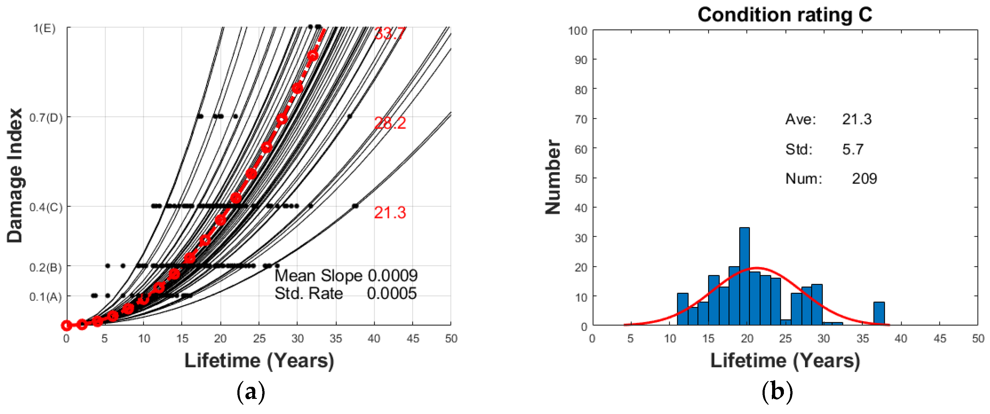
2.2. The Regression Analysis for Each State Condition History Data

The rating of condition history data is classified into five (A, B, C, D, E) grades. Due to being much distributed over the B grade, in the case of regression analysis about all data, the deterioration tendency of practical data cannot be grasped. Thus, the regression analysis was done on processed condition historical data (Figure 2d) for each bridge (or span) and each deterioration rate (slope) was calculated.

Figure 3 indicates the result of regression analysis for each rating of condition history and life-time distribution of the regression equation by C grade. Moreover, the standard deviation rate was calculated in order to consider the uncertainty of the predicted damage index. In this study, the target bridge (to be discussed in detail in Section 4) was the Mokdo Bridge whose superstructure was PSCI girder, which required the development of a deterioration model for the PSCI girders. Further, we performed the regression analysis of the performance history data using each bridge that comprised the PSCI girder among the national highway Type 1 and Type 2 bridges; subsequently, we calculated each deterioration slope. Additionally, to develop the deterioration model using no maintenance action owing to the accelerated deterioration in time, the low rating would result in the acceleration of the deterioration of damage index; we conducted the regression analysis on bridges whose condition history was C or less (D, E grade). This would allow for the realistic implementation of the deterioration characteristics of the aged bridges in operation.

The y-axis of Figure 3a denotes the damage index that is described in the detailed guideline [17]. The x-axis denotes the lifetime (Years = the inspection date of bridge—completion date of bridge) which explains time after damage initiation [4]. The results are obtained from the filtering of the data preprocessing tasks presented in Figure 2 and the bridges with C or lower rating (D, E grade) PSCI girder elements. Figure 3b depicts the C rating data distribution trend of Figure 3a. Furthermore, Figure 3a depicts each deterioration slope based on the regression analysis of each bridge that contains the PSCI girder elements, their mean, and standard deviation deterioration slope, and the duration for reaching the mean deterioration slope by each rating (C rating of 21.3 years). A total of 84 deterioration slopes can be derived from 84 bridges, and their mean deterioration slope can be determined. In case of the deterioration slope calculation for a bridge, the regression determination coefficient (R²) is derived in various shapes, such as the linear, secondary, and exponential curves, based on regression analysis, and the model with the highest regression determination coefficient (R²) was selected as the final deterioration model. The PSCI girder with the aging characteristics that were required in this study was observed to denote the highest regression determination coefficient (R²) in case of the secondary curve regression equation. In other words, there are 84 bridges after data preprocessing; after the calculation and comparison of the regression determinant coefficients (R²) based on each corresponding deterioration slope and three regression equations, their mean deterioration slope was determined. According to these processes, the regression analysis model by condition history for PSCI girder is defined as follows.

$$D.I=a{t}^2+bt+c$$

(1)

In Equation (1), $D.I$ is predicted as damage index, a, b, and c are the regression analysis parameters, t is the lifetime data which was considered from the bridge completion data and inspection data of each rating of condition history. For the uniformity of deterioration and elimination for badness construction of bridge, only the second order polynomial term is considered. Moreover, the characteristic of deterioration is reflected ($a>0$). Therefore, the final regression analysis model for PSCI girder can be defined as Equation (2).

$$D.I=a{t}^2$$

(2)

With this model, the general PSCI girder mean and standard deviation slope are calculated ($a_{mean}^{exi}=8.82\times {10}^{-4}$, $a_{std.dev}^{exi}=4.51\times {10}^{-4}$), also they can be defined as the existing (or initial) deterioration model.

3. Prediction of Bridge Deterioration Progress Based on the Particle Filtering

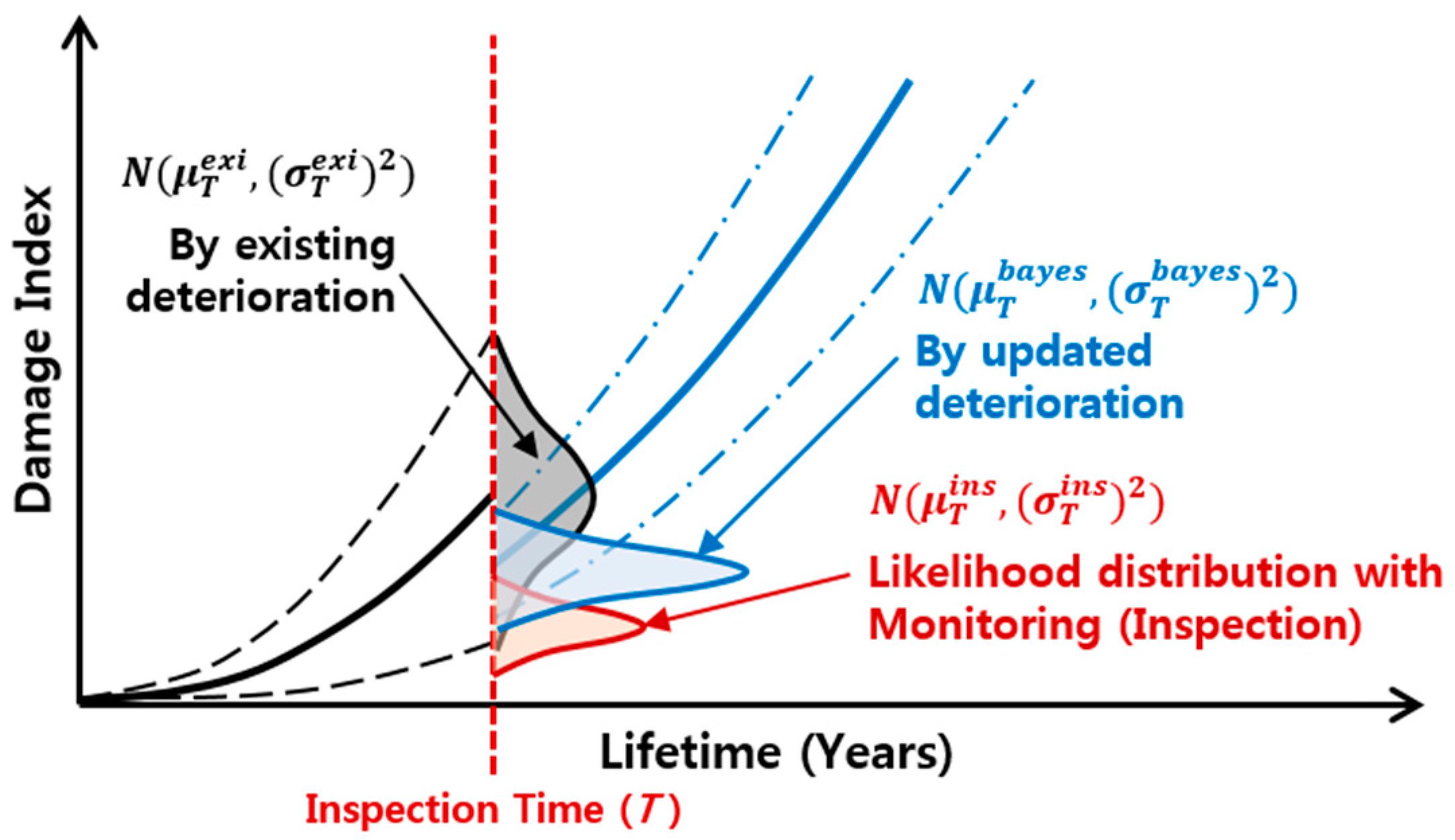
3.1. General Bayesian Updating

The Bayesian updating is considered to be one of the probabilistic methods for updating the existing probability distribution by reflecting the inspection data of the bridge [12]. Moreover, it can be expressed as Equation (3).

$$f\left(\mu |x\right)=cf\left(\mu \right)f\left(x|\mu \right)$$

(3)

where $\mu$ is a value of model parameters, $f\left(\mu \right)$ is a prior probability density function which stands for the uncertainties of deterioration progress according to the prior model parameters. The posterior probability density function that has considered the uncertainties of the inspection data, is denoted by $f\left(\mu |x\right)$ where $x$ is the inspection data. c is defined as a normalizing constant, $f\left(x|\mu \right)$ is the likelihood function that represents the conditional probability of $x$ under the condition model parameters $\mu$. In this research, $\mu$ consists of $a$ for the deterioration model in Equation (2). Additionally, when the prior and likelihood probabilistic density functions follow a normal distribution, the updated posterior probabilistic density function becomes a new normal distribution probabilistic density function. In this case, prior ($f\left(\mu \right)$), likelihood ($f\left(x|\mu \right)$), and posterior function ($f\left(\mu |x\right)$) are described by the following equations of the normal distribution [16,18].

$$f(\mu )\sim N({\mu }_t^{exi}, {({\sigma }_t^{exi})}^2)=\frac{1}{\sqrt{2\pi {({\sigma }_t^{exi})}^2}}exp\left\{\frac{-{(\mu -{\mu }_t^{exi})}^2}{2{({\sigma }_t^{exi})}^2}\right\}$$

(4)

$$f(x|\mu )\sim N({\mu }_t^{ins}, {({\sigma }_t^{ins})}^2)=\frac{1}{\sqrt{2\pi {({\sigma }_t^{ins})}^2}}exp\left\{\frac{-{(x-{\mu }_t^{ins})}^2}{2{({\sigma }_t^{ins})}^2}\right\}$$

(5)

$$f(\mu |x)\sim N({\mu }_t^{bayes}, {({\sigma }_t^{bayes})}^2)=\frac{1}{\sqrt{2\pi {({\sigma }_t^{bayes})}^2}}exp\left\{\frac{-{(\mu -{\mu }_t^{bayes})}^2}{2{({\sigma }_t^{bayes})}^2}\right\}$$

(6)

In Equations (4) to (6), three normal distributions can be found. Here, t is a time of inspection, $N({\mu }_t^{exi}, {({\sigma }_t^{exi})}^2)$ is a normal distribution of damage index by the existing deterioration model with mean and standard deviation, $N({\mu }_t^{ins}, {({\sigma }_t^{ins})}^2)$ is a normal distribution of damage index by the inspection with mean and standard deviation, and $N({\mu }_t^{bayes}, {({\sigma }_t^{bayes})}^2)$ is a normal distribution of damage index by the posterior deterioration model with mean and standard deviation.

As depicted in Figure 4, the damage index data (${\mu }_T^{ins}$, ${\sigma }_T^{ins}$) acquired from the inspection by monitoring the target bridge element at a monitoring point in the time (T). That was determined by the bridge manager of the target bridge that can be used to update the prior probabilistic characteristics (${\mu }_T^{exi}$, ${\sigma }_T^{exi}$) of the previously developed deterioration model (the initial or the existing deterioration model) to the posterior probabilistic characteristics (${\mu }_T^{bayes}$, ${\sigma }_T^{bayes}$) based on the updated deterioration model (updated deterioration model). At this point, the posterior probabilistic characteristics (${\mu }_T^{bayes}$, ${\sigma }_T^{bayes}$) are presented in Equation (7). Moreover, in this case, the standard deviation (${\sigma }_T^{bayes}$) of the updated posterior normal distribution probabilistic density function is always smaller than the standard deviation (${\sigma }_T^{exi}$) of the initial probabilistic density function and the standard deviation (${\sigma }_T^{ins}$) of the likelihood probabilistic density function (Equations (8)) [16,18]. The details of the derivation for Equations (7) and (8) are presented in the Supplementary Materials.

$${\mu }_T^{bayes}=\frac{{\mu }_T^{exi}{\left({\sigma }_T^{ins}\right)}^2+{\mu }_T^{ins}{\left({\sigma }_T^{exi}\right)}^2}{{\left({\sigma }_T^{ins}\right)}^2+{\left({\sigma }_T^{exi}\right)}^2},{\sigma }_T^{bayes}=\sqrt{\frac{{\left({\sigma }_T^{ins}\right)}^2\times {\left({\sigma }_T^{exi}\right)}^2}{{\left({\sigma }_T^{ins}\right)}^2+{\left({\sigma }_T^{exi}\right)}^2}}$$

(7)

$${\sigma }_T^{exi}\ge {\sigma }_T^{bayes}, {\sigma }_T^{ins}\ge {\sigma }_T^{bayes}$$

(8)

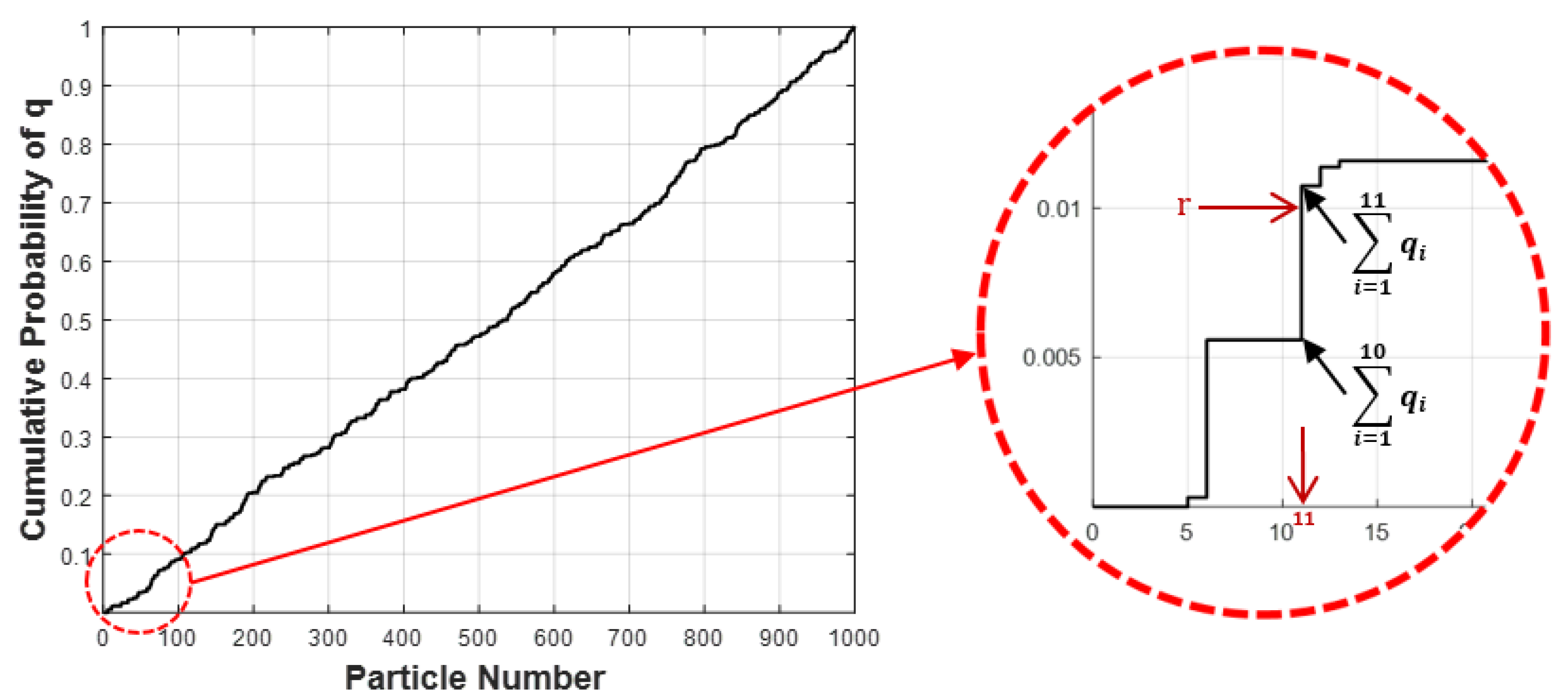
3.2. Particle Filtering Technique

As described in the textbook written by Simon D. [19], the particle filtering technique is a more advanced version of the Bayesian updating based on big data analysis [20]. This technique has been well adapted to nonlinear problems such as the estimation of fatigue crack growth for asphalt concretes [21] and rail wear in Seoul metro [22]. In order to apply the particle filtering technique to the problem considered in this paper, we have set the equations:

$$D.I_k=D.I_{k-1}+a_k{t}^2$$

(9)

$$a_{k+1}=a_k+w_{ak}$$

(10)

$$y_k=D.I_k^{ins}-D.I_k\sim N\left(0,{\sigma }_{D.I}^2\right)$$

(11)

In Equations (9) to (11), $a_k$ is the regression analysis parameter. $w_{ak}$ is white noise vector of 0 (zero)-mean Gaussian. $D.I_k$ is a damage index (D.I) of prediction and t is the lifetime of bridge when $t_0$ is the lifetime of initial inspection. Moreover, $D.I_k^{ins}$ is the measured data by the inspections so, $y_k$ can be defined as the bridge deterioration function with a variance (${\sigma }_{D.I}^2$) which is 0 (zero)-mean Gaussian. As a result, the relative likelihood can be described in Equation (12), as follows.

$$q=P\left(D.I_k^{ins}-D.I_k\right)\sim \frac{1}{\sqrt{2\pi }{\sigma }_{D.I}}exp\left\{-\frac{1}{2}{\left(\frac{D.I_k^{ins}-D.I_k}{{\sigma }_{D.I}}\right)}^2\right\}$$

(12)

Normalize the relative likelihood as below.

$$q_i=\frac{q_i}{{{\displaystyle \sum }}_{j=1}^N{q}_j}$$

(13)

In Equation (13), the summation of all the relative likelihood is 1 (one). N is defined as the number of particles. A new particle can be randomly produced by $q_i$ which can be defined as the relative likelihood. Firstly, a random number (r) is calculated by a uniform probability distribution between 0 and 1. Secondly, $q_i$ is accrued to a sum, by the time the cumulated sum is larger than r [19];

$${\displaystyle \sum }_{i=1}^{j-1}{q}_i<r\le {\displaystyle \sum }_{i=1}^j{q}_i$$

(14)

In Equation (14), $a_j$ can be reselected by this procedure, expressed in Figure 5. The relative likelihood q displays the measurement data. Therefore, when using this procedure, highly probable data are reproduced and those are selected first than other smaller probable data, it means small-weighted data are eliminated and large-weighted data are reproduced. Then, at the next step, the existing particles are replaced by the new particles (N times repetition).

An intuitive schematic explanation is described in Figure 6. Where ${\mu }_k^{PF}$, ${\sigma }_k^{PF}$ are the mean and standard deviation state from particle filtering at k step.

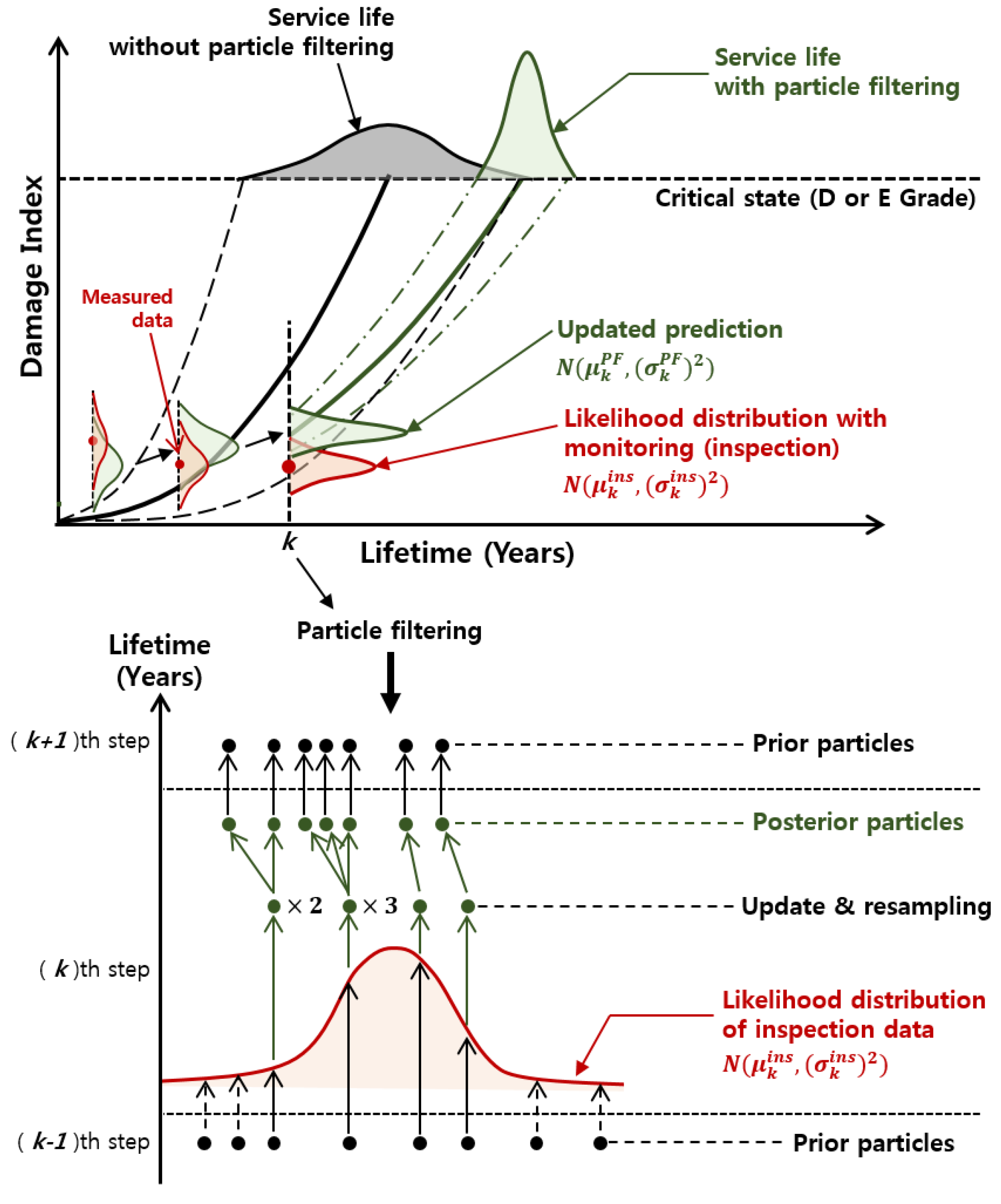
3.3. Particle Filtering Model for Prediction of Bridge Deterioration

To consider this particle filtering method, the bridge inspection data for PSCI girder bridge are used because it has the largest condition history data compared to other types of bridges (i.e., reinforced concrete slab (RCS), rahmen (RA), steel box girder (STB)). Data have been collected by the bridge regular inspection and detecting device. This study has the real dataset of total six-PSCI girder bridges and only those data were chosen for particle filtering analysis that had not been through any maintenance activities, which can affect the bridge repair and reinforcement.

3.4. Application of Particle Filtering Model

The updated parameters, a, and D.I are used for the prediction of deterioration. When the probabilistic characteristic is not given, a uniform distribution is usually applied to the initial distribution [21,22]. The boundaries for the uniform distribution of a was selected based on the regression analysis slope for inspected data and uncertainty ratio of data. The coefficient of variation (C.O.V) of the relative likelihood is assumed to 16%, $w_{ak}$ which is the white noise in Equation (10) [23,24,25]. The $D.I_k$ which is damage index prediction can be obtained with a regression analysis by the particle filtering technique using 1000 (a thousand) particles. The application and verification to the model for the prediction will be shown by the inspection data considered from two measurements of each bridge. In Figure 7, for the more intuitive examination, the 95% confidence interval (CI) of each updating model is presented by the slope which included mean and standard deviation, and the comparison results of prediction uncertainties between using the particle filter and Bayesian method are presented. Comparing the prediction slope or 95% confidential interval and the actual bridge inspection data shows that the prediction model using particle filtering is more reasonable than not only the existing model but also the Bayesian updating prediction model.

Moreover, a relative error is calculated. The relative error (${\epsilon }_{RE}$) is defined as Equation (15),

$${\epsilon }_{RE}=\frac{\left|D.I_{prediction}-D.I_{actual}\right|}{D.I_{actual}}\times 100$$

(15)

where ${\epsilon }_{RE}$ is a relative percentage error between prediction damage index and actual damage index at C (0.4) grade lifetime of each method, $D.I_{prediction}$, $D.I_{actual}$ are the damage index from prediction and actual inspection data, respectively. The ${\epsilon }_{RE}$ according to each bridge is shown in

Table 2. The comparison of uncertainties between particle filtering and Bayesian updating at the time for reaching the actual damage index by C (0.4) grade.

Division	Using Particle Filtering			Using Bayesian
	Mean D.I *	95% CI * of D.I * Lower/Upper	RE	Mean D.I *	95% CI * of D.I * Lower/Upper	RE
Geomyul	0.36	0.301/0.411	10.9%	0.35	0.271/0.423	13.2%
Ha	0.39	0.350/0.433	2.1%	0.42	0.325/0.512	4.7%
Hwangun	0.33	0.272/0.400	17.0%	0.30	0.232/0.363	25.7%
Jangseon	0.34	0.278/0.405	14.7%	0.31	0.239/0.375	23.2%
Mokdo	0.35	0.287/0.405	13.4%	0.28	0.217/0.349	29.2%
Hwangjeon	0.39	0.322/0.458	2.5%	0.35	0.276/0.432	11.6%

* Note: D.I is damage index.; CI is confidence interval; RE is relative error.

. The 95% confidence interval of each bridge is also shown in this table. In Figure 7 and Table 2, all of the PSCI bridges, the uncertainty of the particle filtering updated posterior prediction declined than the Bayesian updating predictions. This is because, the number of updating process based on the particle filtering with the resampling as we already mentioned can reduce the prediction uncertainty.

4. Preventive Maintenance Scenario for Operational Stage Bridge

4.1. Preventive Maintenance

As opposed to the maintenance in the planning stage, the maintenance in the operational stage allows for realistic prediction of the target bridge. The monitoring techniques can detect the damage in the vulnerable parts of the bridge with high precision. Moreover, that can be applied to the existing periodical inspection to select and implement repair and reinforcement methods. In other words, the monitoring techniques can be incorporated into the existing maintenance method to improve the reliability of the target bridge performance prediction. This can lead to a preventive maintenance strategy. The definition and related content of operational stage bridges are described in detail in the literature [16].

4.2. Maintenance Cost Model

The total lifecycle cost of a bridge can be derived from the function of the used materials, including the specifications, environment, and time, and can be generally divided into the initial investment cost, maintenance cost, and the demolition and disposal cost. Here, the maintenance cost is the direct cost that is paid by those who manage the bridge and comprises the periodical inspection cost presented in the detailed guideline, as well as the maintenance cost calculation based on the maintenance scenario analysis. In this study, we considered three expected maintenance cost terms which are the inspection, repair/reinforcement, and rehabilitation (or failure) in this maintenance cost. Furthermore, when the maintenance work is performed, the economic usage of the structure is possible through the improvement of the condition and performance. However, if the optimal maintenance period (or lifetime) is missed, a large-scale construction method or the replacement of the whole structure would be required. To solve these problems, a preventive bridge maintenance scenario strategy needs to be established.

In this study, we considered potential maintenance scenarios for the bridge that is being used and proposed a maintenance cost calculation model that is used for the monitoring techniques in addition to the precise safety diagnosis [23]. The monitoring-based maintenance cost calculation model used the particle filtering technique for updating the existing deterioration model and determining the time for maintenance to predict the maintenance of the target bridge before the damage occurred.

The total expected maintenance cost that is incurred up to a specific lifetime (t) in the general operation stage is formulated in Equation (16);

$$E[C_{MAI,EXI}^{TOT}\left(t\right)]=E[C_{INS,EXI}^{TOT}\left(t\right)]+E[C_{R\&R,EXI}^{TOT}\left(t\right)]+E[C_{F,EXI}^{TOT}\left(t\right)]$$

(16)

$E[C_{MAI,EXI}^{TOT}\left(t\right)]$ denotes the total expected maintenance cost by the existing method which is a function of the specific lifetime (t); $C_{INS,EXI}^{TOT}\left(t\right)$ is the inspection cost; $C_{R\&R,EXI}^{TOT}\left(t\right)$ is the expected repair/reinforcement cost, and $C_{F,EXI}^{TOT}\left(t\right)$ is rehabilitation (or failure) cost. A detailed definition of the three terms is presented in Equations (17) to (19);

$$C_{INS,EXI}^{TOT}\left(t\right)={\displaystyle \sum }_{t=0}^T\frac{1}{{\left(1+q\right)}^t}\{C_{INS,EXI}^{rins}\left(t\right)+C_{INS,EXI}^{pins.}\left(t\right)+C_{INS,EXI}^{psdia}\left(t\right)\}$$

(17)

$$C_{R\&R,EXI}^{TOT}\left(t\right)={\displaystyle \sum }_{i=1}^N\frac{1}{{\left(1+q\right)}^{t_i}}\left\{C_{R\&R,EXI}\left(t_i\right)\times P_{R\&R,EXI}\left(t_i\right)\right\}$$

(18)

$$C_{F,EXI}^{TOT}\left(t\right)={\displaystyle \sum }_{k=1}^K\frac{1}{{\left(1+q\right)}^{t_k}}\left\{C_{F,EXI}\left(t_k\right)\times P_{F,EXI}\left(t_k\right)\right\}$$

(19)

In Equation (17), T is the target lifetime of bridge; the total expected inspection cost is derived as the sum of the regular inspection cost ($C_{INS,EXI}^{rins}\left(t\right)$), precise inspection cost ($C_{INS,EXI}^{pins}\left(t\right)$), and precise safety diagnosis cost ($C_{INS,EXI}^{psdia}\left(t\right)$). In Equation (18), $t_i$ is the time at which the repair and reinforcement methods are applied to the target bridge, and q is the discount rate; $C_{R\&R,EXI}\left(t_i\right)$ and $P_{R\&R,EXI}\left(t_i\right)$ are the repair and reinforcement cost and the repair and reinforcement application probability. In Equation (19), $C_{F,EXI}\left(t_k\right)$ and $P_{F,EXI}\left(t_k\right)$ are the expected rehabilitation (or failure) cost and application probability, respectively; $t_k$ is limit state approaching time which is E grade and after in this paper.

Meanwhile, the total expected maintenance cost for a specific time (t) is when the particle filtering method using monitoring techniques ($E[C_{MAI,PF}^{TOT}\left(t\right)]$) is defined in Equation (20). Moreover, a detailed definition of three terms is presented in Equations (21) to (23);

$$E[C_{MAI,PF}^{TOT}\left(t\right)]=E[C_{INS,PF}^{TOT}\left(t\right)]+E[C_{R\&R,PF}^{TOT}\left(t\right)]+E[C_{F,PF}^{TOT}\left(t\right)]$$

(20)

$$C_{INS,PF}^{TOT}\left(t\right)=C_{SEN}\left(t_0\right)+{\displaystyle \sum }_{t=0}^T\frac{1}{{\left(1+q\right)}^t}\{C_{INS,EXI}^{rins}\left(t\right)+C_{INS,EXI}^{pins.}\left(t\right)+C_{INS,PF}^{psdia}\left(t\right)\}$$

(21)

$$C_{R\&R,PF}^{TOT}\left(t\right)={\displaystyle \sum }_{i=1}^N\frac{1}{{\left(1+q\right)}^{t_i}}\left\{C_{R\&R,PF}\left(t_i\right)\times P_{R\&R,PF}\left(t_i\right)\right\}$$

(22)

$$C_{F,PF}^{TOT}\left(t\right)={\displaystyle \sum }_{k=1}^K\frac{1}{{\left(1+q\right)}^{t_k}}\left\{C_{F,PF}\left(t_k\right)\times P_{F,PF}\left(t_k\right)\right\}$$

(23)

In Equation (20), $E[C_{MAI,PF}^{TOT}\left(t\right)]$ denotes total expected maintenance cost by particle filtering method which is the function of the specific lifetime (t); $C_{INS,PF}^{TOT}\left(t\right)$ is the inspection cost; $C_{R\&R,PF}^{TOT}\left(t\right)$ is the expected repair/reinforcement cost, and $C_{F,PF}^{TOT}\left(t\right)$ is rehabilitation (or failure) cost. In Equation (21), $C_{SEN}\left(t_0\right)$ denotes the initial ($t_0$) sensor installation cost, and $C_{INS,PF}^{psdia}\left(t\right)$ is derived from the sum of the precise safety diagnosis cost. In Equation (22), $C_{R\&R,PF}\left(t_i\right)$ is the repair and reinforcement method cost linked to the updated deterioration model at the repair and reinforcement application time ($t_i$) of the target bridge, $P_{R\&R,PF}\left(t_i\right)$ is the repair and reinforcement implementation probability linked to the updated deterioration model at the time ($t_i$); In Equation (23), $C_{F,PF}\left(t_k\right)$ and $P_{F,PF}\left(t_k\right)$ are the expected rehabilitation (or failure) cost and application probability.

In calculating the maintenance cost incurred in the actual bridge, the proposed preventive maintenance cost analysis method with the monitoring technique-based particle filtering is advantageous. This is because the particle filtering technique is used to reduce the uncertainty (${\sigma }_t^{exi}$) of the existing deterioration model in the life cycle management analysis. In addition, the comparison of the maintenance cost before and after the monitoring-based particle filtering update denotes that the monitoring-based preventive maintenance is more advantageous than not only using the existing maintenance method, but also using Bayesian method in terms of cost efficiency.

5. Effects of Proposed Method

5.1. Mokdo Bridge and Input Parameters

To propose the applicability and reasonability of the particle filtering method-based preventive Bridge maintenance scenario strategy, we selected the PSCI girder of the Mokdo Bridge, which is the high risk case when the largest differences of uncertainty is calculated between using Bayesian and using particle filtering (Figure 7 and Table 2). The general specifications of the target bridge are presented in

Table 3. Generation information on the target bridge: Mokdo Bridge.

Division	Quantity	Division	Quantity
Bridge Type	PSCI girder	Number of Girder	5
Design Load	DB-24 *	Number of Lane	2
Number of Span	4	Span Length (m)	30
Completion Date	1998.12.01	Total Span Length (m)	120(4@30)
PC Tendon (EA)	80(5@4@4)	Effectiveness Width (m)	10.5

* Note: DB-24 is the standard design vehicle loads in Korea.

.

5.2. Maintenance Cost Model Applied to the Target PSCI Girder Bridge

The eddy-current sensor (ECS) technique generates eddy current on a target surface through a magnetic field, and investigates the eddy current variation with condition changes of the target surface. The magnetostriction effect is defined as a variation of the magnetic permeability due to an alteration of stress level in ferromagnetic materials. Through it, the stress levels of the wedge surface alters its magnetic permeability, causing an amplitude variation of the eddy current on post-tensioning (PT) anchorage. The tension force loss detection ECS technology detects the variation of tension force on PSC bridges, and prevents large accidents and casualties that are caused by the tension force reduction. The ECS technique has many advantages (low cost, simple installation, low power consumption, and automatic warning) [23,26,27].

By reflecting on the accuracy of the ECS technique, the inspection error (${\sigma }_t^{ins}$) was assumed to be 0.05 (95% of accuracy) which is high quality inspection [24,25], and the initial ECS cost used the information that is presented in

Table 4. Assumption of ECS sensor.

Division	Quantity
Cost of unit of ECS sensor including installation (KRW)	400,000
The number of ECS (EA)	480
Probability of misclassification using ECS (%)	5

; further, each inspection cost that is based on the existing method and on the sensor is presented in

Table 5. Comparison between existing inspection method and inspection using ECSs.

Division	Regular Inspection		Precise Inspection		Precise Safety Diagnosis
	Existing	ECSs	Existing	ECSs	Existing	ECSs
One-time Inspection Cost ($\times {10}^3$ KRW)	3437		16,152		48,463	26,450
Inspection Time	Once every six months		Once every two years		(First time in 10 years) Once every five years

. The discount rate was set to 1.01% by reflecting the actual discount rate for a decade by economic statistics system (ECOS) in the bank of Korea. The initial ($t_0$) sensor installation cost is [$C_{SEN}\left(t_0\right)=\mathrm{400,000}KRW\times 8\left(anchorages per girder\right)\times$ $3\left(ECS per anchorage\right)\times 5\left(girder\right)\times 4\left(span\right)=\mathrm{192,000,000}KRW$] in Equation (21). Three ECSs as depicted in Figure 8 were assumed to be installed in both ends of the anchorages for the girder (Figure 9). Due to the advantages above-mentioned (especially, automated warning), when using ECSs, the direct labor cost was assumed to about 50% of the existing maintenance direct labor cost in precise safety diagnosis [23]. In addition, by referring to the precise inspection and precise safety diagnosis cost (cost calculation) (Notice of the Ministry of Land, Infrastructure, and Transport (revised on 12.06, 2016)), we proposed each inspection cost for the existing method and for the use of the sensor (regular inspection cost, precise inspection cost, and precise safety diagnosis cost) as presented in Table 5 [23].

Meanwhile, we developed a condition rating improvement model using the condition rating improvement data of the repair and reinforcement list calculated using the results of the maintenance record DB of KICT BMS and also based on the specialists’ opinions [28]. In this study, we determined three major repair and reinforcement methods (

Table 6. Repair and reinforcement cost input data of the Mokdo PSCI girder.

Representative Damage Type	Representative Application Method	Unit Cost (KRW)	Application Grade	Application Frequency Rate (%)	Cost of Maintenance by Rating (KRW)
Exposed, corroded tendons	Filling method (Grouting)	173,134	B(0.2)	62.0	16,361,000
			C(0.4)	29.5	629,704,000
	External post-tensioning	2,837,937	C(0.4)	16.0
			D(0.7)	22.0	2,096,940,000
tendon fractures	Girder replacement	7,969,380	D(0.7)	25.0
			E(1)	100.0	3,785,615,000

) applicable to exposed, corroded tendons and tendon fractures and linked these three methods to each condition improvement cost. Figure 10 depicts the maintenance cost per condition rating of the PSCI girder of the Mokdo Bridge and whose cubic polynomial curve tendency is based on the regression analysis of the cumulative maintenance cost per rating. Here, the cost rapidly increases with the low rating (D, E grade), and this is because the low rating (D, E grade) causes the application of methods with a high unit cost, including external post-tensioning and girder replacement [28]. Moreover, the cubic polynomial regression function is shown in Figure 10 based on Table 6.

5.3. Discussions Based on the Results of the Maintenance Cost

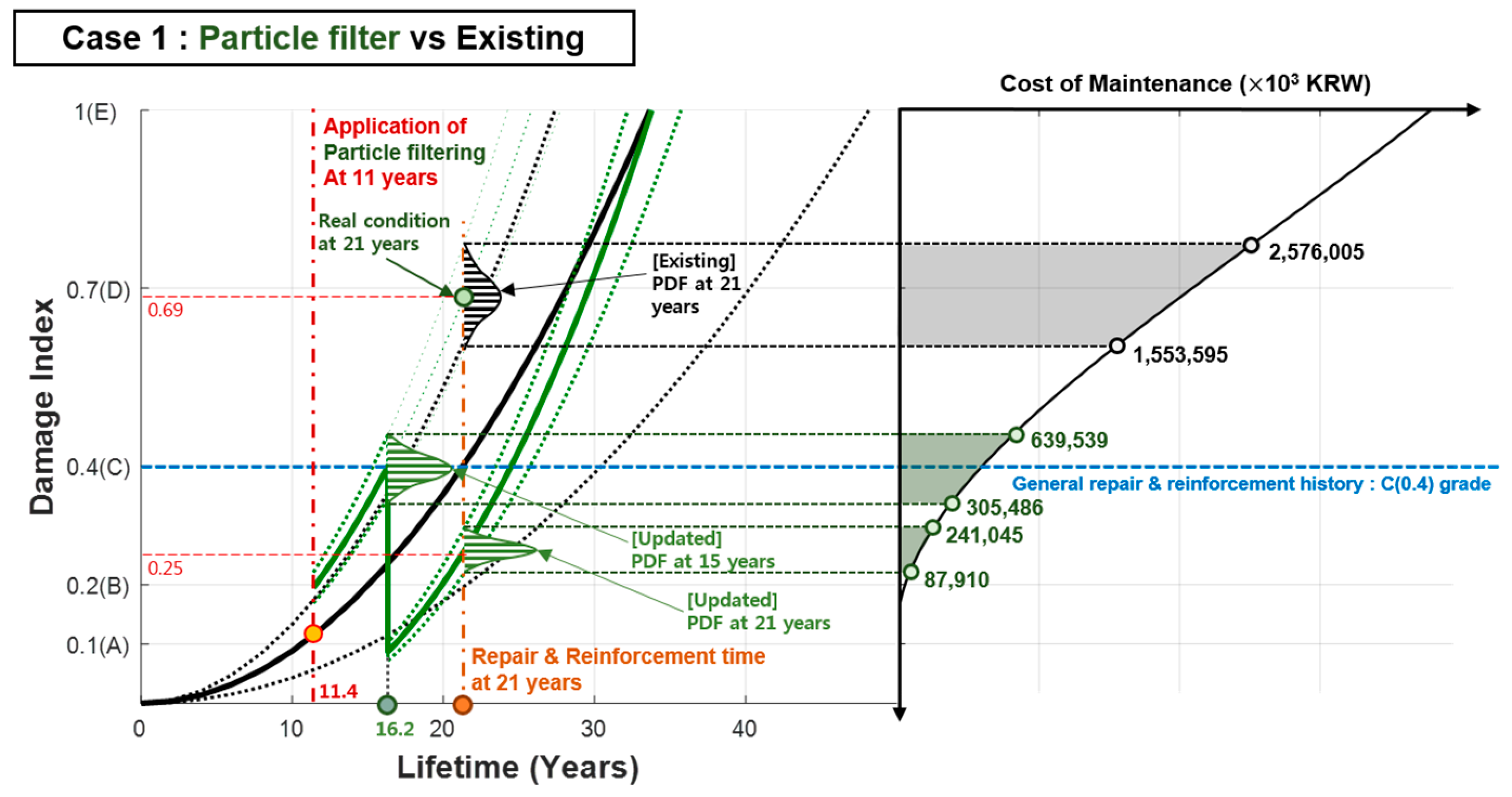
The results of the maintenance cost calculated by the particle filter technique were compared to those calculated by the existing technique. In case of the particle filtering update with the monitoring technology when compared to the existing maintenance scenario, the update is possible by detecting the damages, such as tension force loss, in the early stage of the operation of the bridge so as to reduce the uncertainty of the bridge deterioration model. In this study, it was quantitatively proved that the proposed method was more efficient with two major maintenance scenarios in such an operational stage (Cases 1, 2). Especially, the real bridge data set and prediction model are reflected in Case 2.

The particle filtering updating time using the two major maintenance scenarios (Case 1, 2) was set to eleven years, which was the real inspection datum (Figure 7e) reflected; this is because the tension force loss at the end of the PSCI girder, the places as ECS installation locations (Figure 9), may occur during or after the precise safety diagnosis is required [26,27].

5.3.1. Case 1: Updated Mean State (${\mu }_t^{PF}$) < Existing Mean State (${\mu }_t^{exi}$)

By considering the real case in which the mean slope ($a_{mean}^{PF}=1.53\times {10}^{-3}$) of the particle filtering updated deterioration model tends to follow the deterioration slope close to the lower limit of the existing deterioration model at the particle filtering update point (11.4 years) that is applied with the ECSs, and this Case 1 is reflected in the real PSCI bridge (Mokdo bridge) inspection data which is already mentioned in Section 3.4. As depicted in Figure 11, when we only know the existing deterioration model, the condition of the actual target PSCI bridge is not predicted. Accordingly, the repair and reinforcement cost is applied not in the C rating (0.4) but in a rating closer to D rating (0.69).

Figure 11 also depicts the potential scenario based on the particle filtering update based deterioration model with ECSs. The particle filtering algorithm (Equations (9) to (14)) is used to calculate the revised deterioration model (${\mu }_{11.4}^{PF}=0.198,{\sigma }_{11.4}^{PF}=0.029$) of the Mokdo bridge PSCI girder through the particle filtering update in eleven years with the ECS technique; further, it considers the repair and reinforcement method application probability as well as cost (Equation (22)) when the update deterioration model reaches the C rating (0.4; 16 years), which is the target maintenance level (C rating (0.4)). As has been discussed, the monitoring shows that the deterioration of the PSCI girder of the target bridge advances more rapidly when compared to the existing inspection; accordingly, an accurately targeted maintenance level (C rating: 0.4; 16 years) is calculated. Each repair and reinforcement cost at the corresponding rating (0.4) is calculated by multiplying the repair and reinforcement application probability ([$P_{R\&R,PF}\left(16.2\right)$]) and using the matched repair and reinforcement method cost ([$C_{R\&R,PF}\left(16.2\right)$]). Moreover, each repair and reinforcement cost at the corresponding mean rating (0.25) is calculated by multiplying the repair and reinforcement application probability ([$P_{R\&R,PF}\left(21\right)$]) and using the matched repair and reinforcement method cost ([$C_{R\&R,PF}\left(21\right)$]) that are considered.

According to Case 1 in

Table 7. Comparison between total maintenance cost of existing ($E[C_{MAI,EXI}^{TOT}\left(21\right)]$) and particle filtering ($E[C_{MAI,PF}^{TOT}\left(21\right)]$) for 21 years.

Division	Cost (Unit: KRW)
	Inspection	Repair and Reinforcement	Rehabilitation (Failure)	Total Maintenance
Existing Scenario	334,952,646	1,663,780,152	1,013,611	1,999,746,409
PF Scenario	470,106,591	530,423,653	9.93$\times {10}^{-21}$	1,000,530,244

, the total maintenance cost for 21 years before and after the particle filtering update was calculated by Equations (16) and (20), denoting approximately 50% of the cost-saving effect. If the updated mean condition (${\mu }_{11.4}^{PF}=0.198$) is larger than the existing prediction condition (${\mu }_{11.4}^{exi}=0.115$), the reasons for such maintenance cost saving (−999,216,166 KRW) are as follows.

While considering the maintenance scenario using the ECS applied monitoring technology, the condition of the target PSCI girder in eleven years, the time at which the particle filtering update is performed, is determined to be worse than the initial condition, and the time at which the update condition reaches the target maintenance level (C rating (0.4)) can be accurately predicted. If the existing maintenance scenario cannot predict the condition of the actual PSCI girder; accordingly, one repair and reinforcement cost close to D rating (0.69) would occur in 21 years. Furthermore, the existing maintenance scenario has come close to E rating (1.0) and it is possible to increase the rehabilitation cost (1,013,611 KRW) which can be calculated by Equation (19). However, if the condition of the ECS applied particle filtering update-based target structure is accurately predicted, the maintenance scenario plan based on the updated deterioration model would result in one repair and reinforcement cost corresponding to C rating (0.4) in 16 years. According to this preventive maintenance scenario, the rehabilitation cost (9.93 $\times {10}^{-21}$ KRW) is almost equal to zero by Equation (23).

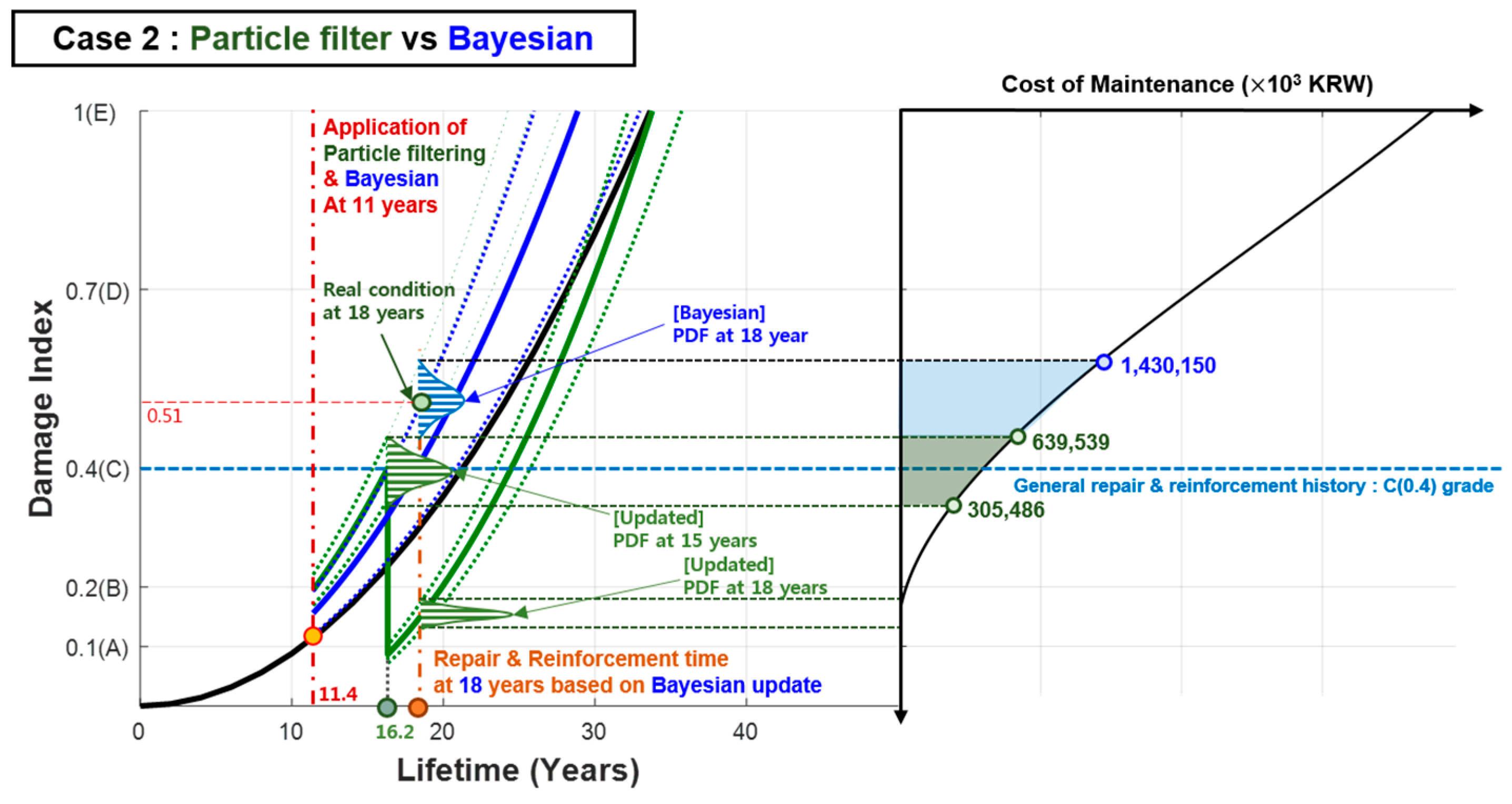
5.3.2. Case 2: Comparison to the Bayesian Updating Model

In this section, we considered the real case in which the mean slope of the updated deterioration model tends to follow the deterioration slope ($a_{mean}^{PF}=1.53\times {10}^{-3}$) close to the lower limit of the existing deterioration model at the particle filtering update point (11.4 years) that is applied with the ECSs, and this case is reflected in real PSCI bridge (Mokdo Bridge) inspection data which is already mentioned in Section 3.4. As depicted in Figure 12, when we know the existing and Bayesian deterioration model, the condition of the actual target PSCI bridge can be predicted, but, as we already considered in Figure 7 and Table 2, the Mokdo PSCI Bridge deterioration model based on general Bayesian updating method still has uncertainties when compared to the application of particle filtering method. Accordingly, the maintenance cost can be applied not in the C rating (0.4) but in the rating closer to the range of D rating (0.51) which was mentioned in Table 1. Figure 12 also depicts the potential scenario based on the particle filtering update with deterioration model using ECSs. The particle filtering algorithm (Equations (9) to (14)) is used to calculate the updated deterioration model (${\mu }_{11.4}^{PF}=0.198,{\sigma }_{11.4}^{PF}=0.029$) of the Mokdo Bridge PSCI girder through the particle filtering update in eleven years with the ECS technique; further, it considers the repair and reinforcement method application probability as well as cost when the update deterioration model reaches the C rating (0.4; 16 years), which is the target maintenance level. Meanwhile, if the Bayesian updating technique is applied, the Bayesian updated deterioration model can be calculated by Equation (7), which is the mean and standard deviation value at eleven years (${\mu }_{11.4}^{bayes}=0.159,{\sigma }_{11.4}^{bayes}=0.034$). Each repair and reinforcement cost at the corresponding rating (0.4) is calculated by multiplying the repair and reinforcement application probability ([$P_{R\&R,bayes}\left(16.2\right)$]) and using the matched repair and reinforcement method cost ([$C_{R\&R,bayes}\left(16.2\right)$]). Moreover, each repair and reinforcement cost at the corresponding mean rating (0.15) is calculated by multiplying the repair and reinforcement application probability ([$P_{R\&R,bayes}\left(18\right)$]) and using the matched repair and reinforcement method cost ([$C_{R\&R,bayes}\left(18\right)$]) that are considered.

According to Case 2 which is compared between particle filtering and Bayesian updating in

Table 8. Comparison between total maintenance cost of Bayesian ($E[C_{MAI,bayes}^{TOT}\left(18\right)]$) and particle filtering ($E[C_{MAI,PF}^{TOT}\left(18\right)]$) for eighteen years.

Division	Cost (Unit: KRW)
	Inspection	Repair and Reinforcement	Rehabilitation (Failure)	Total Maintenance
Bayesian Scenario	434,373,456	911,667,506	2.45 $\times {10}^{-4}$	1,346,040,961
PF Scenario		525,544,859	1.01 $\times {10}^{-20}$	959,918,315

, the total maintenance cost for eighteen years before and after the particle filtering update was calculated by Equation (20) because of the same inspection cost, denoting approximately 29% of the cost-saving effect. If the updated mean condition (${\mu }_{11.4}^{PF}=0.198$) is larger than the existing prediction condition (${\mu }_{11.4}^{bayes}=0.159$), the reasons for such maintenance cost saving (−386,122,647 KRW) are as follows. The condition of the target PSCI girder in eleven years, the time at which the particle filtering update is performed, is determined to be worse than the condition based on Bayesian updating, and the time at which the particle filtering update condition reaches the target maintenance level (C rating (0.4)) can be accurately predicted. If the Bayesian applied maintenance scenario cannot predict the condition of the Mokdo PSCI girder; accordingly, one repair and reinforcement cost close to D rating (0.51) would occur in eighteen years. However, if the condition of the ECS applied particle filtering update-based target structure is accurately predicted, the maintenance scenario plan based on the updated deterioration model would result in one repair and reinforcement cost corresponding to C rating (0.4) in sixteen years.

6. Conclusions

With the recent expansion of the maintenance market because of an increase in the number of aged bridges in South Korea, there has been a growing requirement for studies on advanced maintenance management strategies.

Intending to establish a model with a practical application of the bridge condition and performance changes over time during establishing a maintenance scenario strategy, we developed a deterioration model based on the secondary function, which allowed for maintaining the initial condition of bridges that were being used and the reflection of the acceleration zones.

In addition, the deterioration model was estimated in the designing and planning stage through the particle filtering technique that could be updated by probabilistically combining the damage inspection data results acquired from the eddy-current sensor (ECS) based monitoring techniques. Through the developed secondary function-based deterioration model, an accurate condition of the target bridge (element) can be predicted so as to reduce the repair and reinforcement cost during necessary periods, which means that a systematic and efficient maintenance control can be observed during the service life in the operational stage of the bridge. The installation of a continuously advancing monitoring device for inspecting the vulnerable parts of a bridge would cause initial costs; however, it can reduce the direct labor cost that is required for performing the current visual inspection, and the improvement of the accuracy of the updated deterioration model through the particle filtering technique can allow for the establishment of a preventive maintenance plan in the mid/long-term operational stage; accordingly, a considerable amount of repair and reinforcement cost can be saved. In this study, we made the following three main conclusions:

(1)

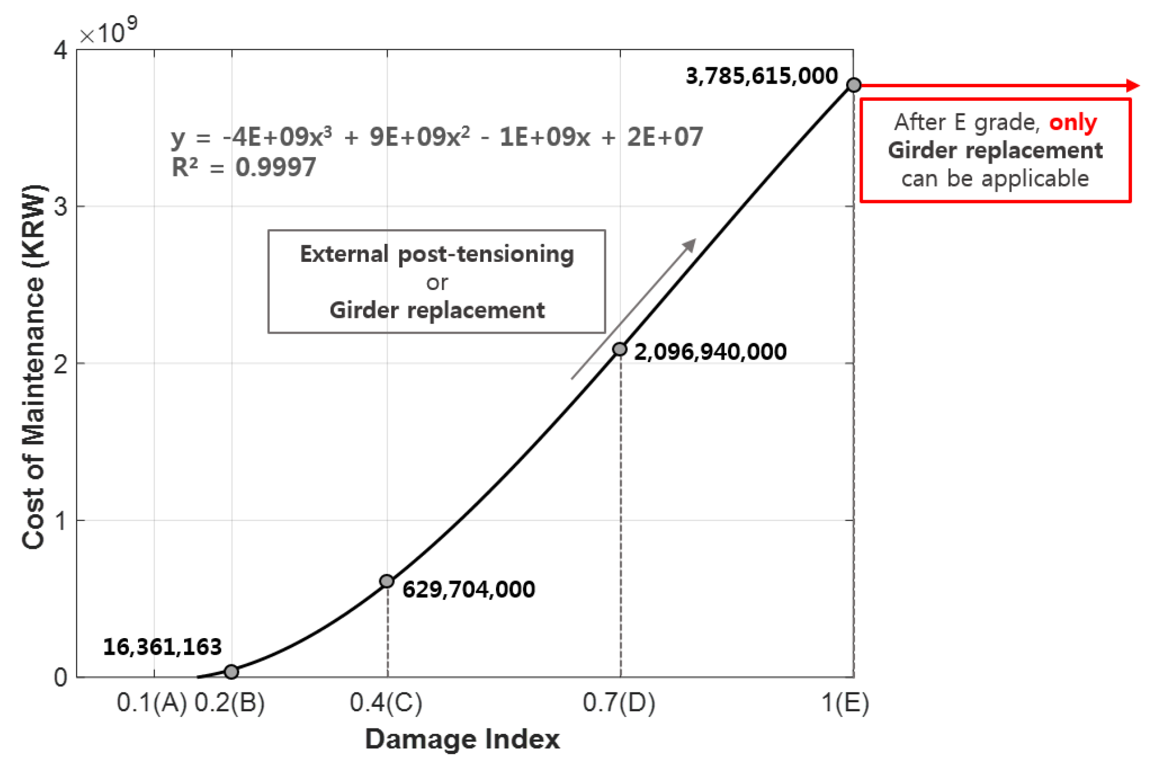
This study proposed potential maintenance scenarios (Case 1 and 2) by considering the particle filtering update based on big data using the monitoring technologies in the operational stage of the bridge that is currently in use and applying it to the specific element of the Mokdo Bridge (PSCI girder) so as to determine the cost saving because of the update for the existing deterioration model based on the general maintenance level setting (C rating). It was analyzed that such cost saving can be attributed to the increase in the maintenance cost (Figure 10), where the acceleration trend of the cubic polynomial curve was reflected more as the rating of the PSCI girder fell (D, E grade).

(2)

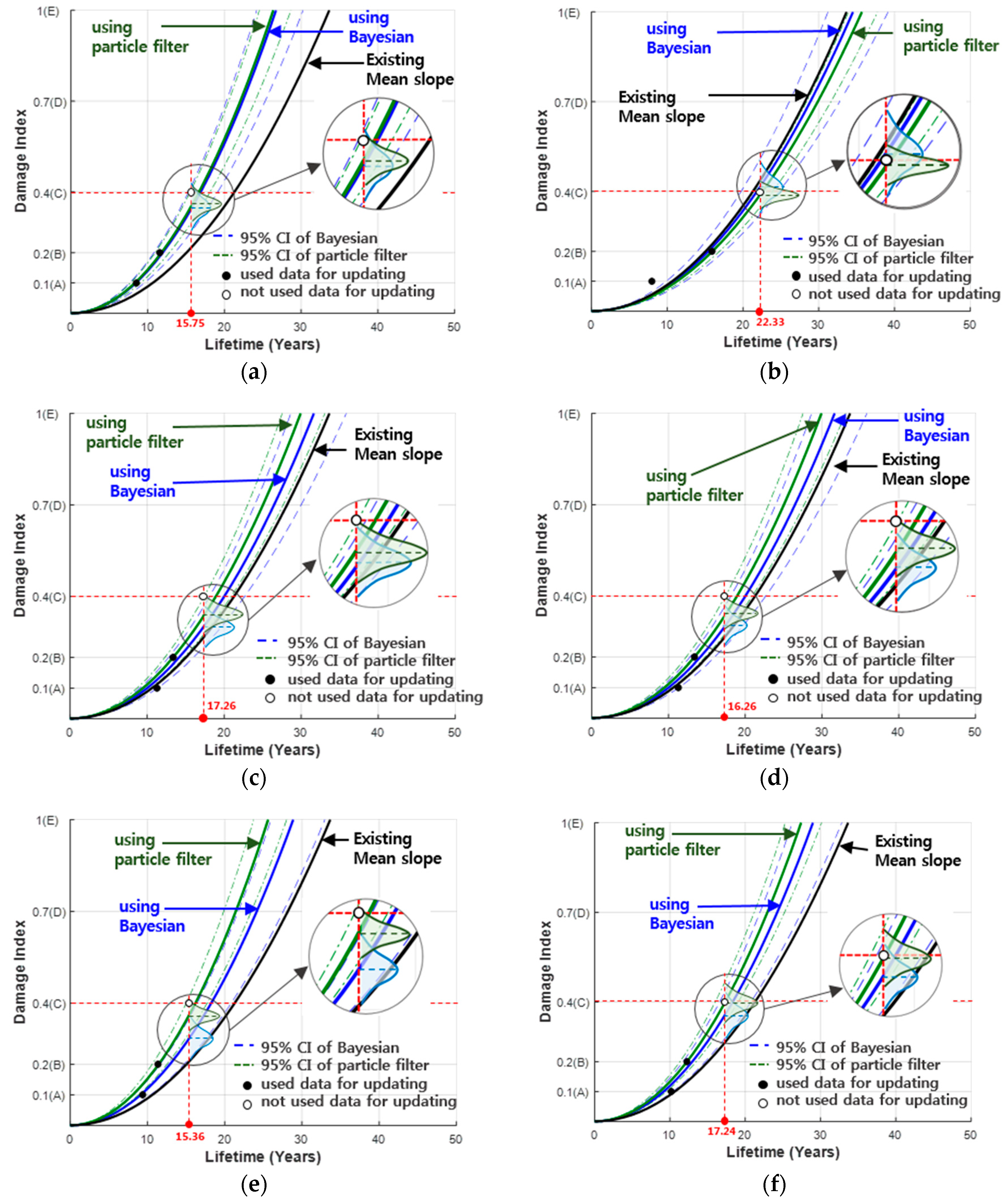
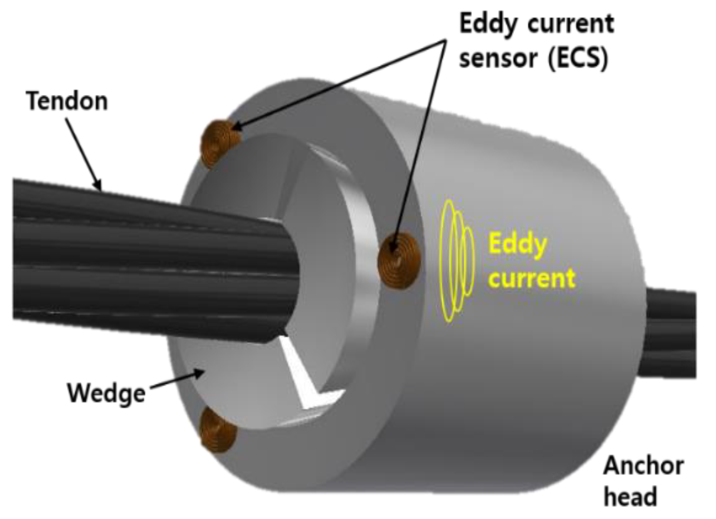
According to the example in (Section 5.3) for calculating the maintenance cost, which was considered in this study, the maintenance level of the bridge (rating) was set to C rating (0.4), and the particle filter update was performed for a specific time (eleven years). Case 1 showed a steeper slope when compared to that of the existing deterioration model, resulting in approximately 50% of the maintenance cost-saving effect. This was because the proposed model detected damage types, such as pre-stressed tendon, which could be difficult to detect using the existing visual inspection and nondestructive inspection, and allowed for the early prediction of posterior damages and the subsequent one-time preventive repair and reinforcement.

(3)

The proposed preventive bridge maintenance scenario using the particle filtering estimation broke away from the current maintenance system, where maintenance action is performed after the damages were detected by the inspection of almost D rated (0.69) bridges and where the condition of the maintenance target structures was accurately predicted. Thus, we presented the potential application of the proposed model for establishing a maintenance decision-making process, including the determination of the optimal repair and reinforcement period. It is expected that the particle filtering update-based maintenance scenario using monitoring technologies, which was proposed in this study, could save a considerable amount of repair and reinforcement cost when compared to the existing labor-based maintenance strategies, which could not determine the causes of early deterioration.

References

1. Lake, N.; Seskis, J. Bridge Management Using Performance Models; Technical Report; Austroads: Sydney, Australia, 2013. [Google Scholar]
2. Emotoa, H.; Takahashib, J.; Widyawatic, R.; Miyamoto, A. Performance evaluation and remaining life prediction of an aged Bridge by J-BMS. Procedia Eng. 2014, 95, 65–74. [Google Scholar] [CrossRef]
3. Thompson, P.D.; Small, E.P.; Johnson, M.; Marshall, A.R. The Pontis Bridge Management System. Struct. Eng. Int. 2018, 8, 303–3008. [Google Scholar] [CrossRef]
4. Enright, M.P.; Frangopol, D.M. Condition Prediction of Deteriorating Concrete Bridges using Bayesian Updating. J. Struct. Eng. 1999, 125, 1118–1125. [Google Scholar] [CrossRef]
5. Zonta, D.; Zandonini, R.; Bortot, F. A reliability-based bridge management concept. Struct. Infrastruct. Eng. 2007, 3, 215–235. [Google Scholar] [CrossRef]
6. Catbas, F.N. Structural health monitoring: Applications and data analysis. In Structural Health Monitoring of Civil Infrastructure Systems; Woodhead Publishing: Cambridge, UK, 2009; pp. 1–39. [Google Scholar]
7. Zhang, R.; Castel, A.; Francois, R. The corrosion pattern of reinforcement and its influence on serviceability of reinforced concrete members in chloride environment. Cem. Concr. Res. 2009, 39, 1077–1086. [Google Scholar] [CrossRef]
8. Zubair, M.; Zhang, Z.; Salah, U.K. Reliability Data Update Method with Gamma Distribution. In Proceedings of the 2011 Asia-Pacific Power and Energy Engineering Conference, Wuhan, China, 25–28 March 2011; pp. 1–4. [Google Scholar]
9. Orcesi, A.D.; Frangopol, D.M. Bridge Performance Monitoring Based on Traffic Data. J. Eng. Mech. 2013, 139, 1508–1520. [Google Scholar] [CrossRef]
10. Ferreira, C.; Neves, L.; Matos, J.; Soares, J.S. A degradation and maintenance model: Application to Portuguese context. In Proceedings of the 7th International IABMAS Conference on Bridge Maintenance, Safety, Management, Resilience and Sustainability, Shanghai, China, 7–11 July 2014. [Google Scholar]
11. Korea Agency for Infrastructure Technology Advancement (KAIA). Large-Scale Infrastructure Monitoring and Management Using Unmanned Inspection Units; KAIA: Anyang-Si, Korea, 2016.
12. Zampieri, P.; Curtarello, A.; Pellegrino, C.; Maiorana, E. Fatigue strength of corroded bolted connection. Frat. Ed Integr. Structturale 2018, 12, 90–96. [Google Scholar] [CrossRef]
13. Lee, C.Y.; Lee, M.K. Demand Forecasting in the Early Stage of the Technology’s Life Cycle Using a Bayesian Update. Sustainability 2017, 9, 1378. [Google Scholar] [CrossRef]
14. Lee, C.Y.; Huh, S.Y. Forecasting Long-Term Crude Oil Prices Using a Bayesian Model with Informative Priors. Sustainability 2017, 9, 190. [Google Scholar] [CrossRef]
15. Asadollahi, P.; Huang, Y.; Li, J. Bayesian Finite Element Model Updating and Assessment of Cable-Stayed Bridges Using Wireless Sensor Data. Sensors 2018, 18, 3057. [Google Scholar] [CrossRef] [PubMed]
16. Lee, J.H.; Choi, Y.R.; Ann, H.; Kong, J.S. The Preventive Maintenance Strategy in Operation Stage of Bridge using Bayesian Inference. J. Korea Soc. Civ. Eng. 2019, 39, 135–146. [Google Scholar]
17. Technical Report; Guideline and Commentary of Safety Inspection and In-Depth Safety Inspection for Structures-Bridge; Korea Infrastructure Safety & Technology Corporation (KISTEC): Seoul, Korea, 2017.
18. Ang, A.; Tang, W. Probability Concepts in Engineering: Emphasis on Applications in Civil and Environmental Engineering, 2nd ed.; Willey: Hoboken, NJ, USA, 2007; pp. 346–365. [Google Scholar]
19. Simon, D. Optimal State Estimation: Kalman, H-Infinity, and Nonlinear Approaches; John Willey & Sons: Hoboken, NJ, USA, 2006; pp. 461–483. [Google Scholar]
20. Dowd, M.; Joy, R. Estimating behavioral parameters in animal movement models using a state-augmented particle filter. Ecology 2011, 92, 568–575. [Google Scholar] [CrossRef] [PubMed]
21. Lee, S.J.; Zi, G.; Mun, S.; Kong, J.S.; Choi, J.H. Probabilistic prognosis of fatigue crack growth for asphalt concretes. Eng. Fract. Mech. 2015, 141, 212–229. [Google Scholar] [CrossRef]
22. Jeong, M.C.; Lee, S.J.; Cha, K.; Zi, G.; Kong, J.S. Probabilistic model forecasting for rail wear in seoul metro based on Bayesian theory. Eng. Fail. Anal. 2019, 96, 202–210. [Google Scholar] [CrossRef]
23. Sohn, H. Bridge Life-Span Extension Using ICT, Partial Replacement and Low-Carbon Materials; Technical Report; Korea Agency for Infrastructure Technology Advancement (KAIA): Anyang, Korea, 2018.
24. Frangopol, D.M.; Neves, L. Structural Performance Updating and Optimization with Conflicting Objectives under Uncertainty. ASCE J. Struct. Eng. 2008. [Google Scholar] [CrossRef]
25. Sun, J.W.; Park, K.H.; Kwang, J.K.; Kong, J.S.; Park, D.H. Study on Bayesian Probability Model for Estimation of Bridges Performance. In Proceedings of the 2010 Korean Society of Civil Engineers Conference, Incheon, Korea, 20–22 October 2010; pp. 1345–1348. [Google Scholar]
26. Kim, J.-M.; Lee, J.; Sohn, H. Automatic measurement and warning of tension force reduction in a PT tendon using eddy current sensing. NDT E Int. 2017, 87, 93–99. [Google Scholar] [CrossRef]
27. Kim, J.-M.; Lee, J.; Sohn, H. Detection of tension force reduction in a post-tensioning tendon using pulsed-eddy-current measurement. Struct. Eng. Mech. 2018, 65, 129–139. [Google Scholar]
28. Hwang, Y.K. Developing Bridge. Management System considering Life-Cycle Cost and Performance of Bridges; Technical Report; Ministry of Land, Transport and Maritime Affairs (MLTMA): Gwacheon, Korea, 2008.
Figure 1. Flow chart of preventive maintenance cost estimation by eight steps.
Sustainability 11 06593 g001
Figure 2. The process step of the condition rating data for PSCI girder. (a) Data distribution before processing; (b) remove the error data or repeated data; (c) remove the data which have the maintenance measure; (d) remove the condition history data which is only 1.
Sustainability 11 06593 g002
Figure 3. PSCI girder for deterioration model and lifetime distribution at C (0.4) grade. (a) The regression analysis by condition history for PSCI girder; (b) lifetime distribution at C (0.4) damage index for PSCI girder.
Sustainability 11 06593 g003
Figure 4. Schematic of the Bayesian update based on the existing deterioration model.
Sustainability 11 06593 g004
Figure 5. Resampling of the particle filter; for example, if a random number r = 0.01 , the smallest value of j for Equation (14) is 11; a 11 is reselected.
Sustainability 11 06593 g005
Figure 6. Schematic of the particle filtering method.
Sustainability 11 06593 g006
Figure 7. The prediction of each PSCI girder bridge in which each of the full lines show the mean slopes of prediction. (a) The Geomyul PSCI girder bridge. (b) The Ha PSCI girder bridge. (c) The Hwangun PSCI girder bridge. (d) The Jangseon PSCI girder bridge. (e) The Mokdo PSCI girder bridge. (f) The Hwangjeon PSCI girder bridge.
Sustainability 11 06593 g007
Figure 8. Three-dimensional schematic of eddy-current sensor (ECS) installation on an anchor head.
Sustainability 11 06593 g008
Figure 9. The installation locations of ECSs in the Mokdo Bridge. (a) The longitude section view. (b) The cross-sectional view. (c) The edge of beam detail.
Sustainability 11 06593 g009
Figure 10. Maintenance cost model applied to the Mokdo PSCI girder.
Sustainability 11 06593 g010
Figure 11. [Case 1] Existing and updated deterioration and cost of maintenance by damage index.
Sustainability 11 06593 g011
Figure 12. [Case 2] Bayesian and particle filtering deterioration and cost of maintenance by damage index.
Sustainability 11 06593 g012