Article

Flood Vulnerability Assessment through Different Methodological Approaches in the Context of North-West Khyber Pakhtunkhwa, Pakistan

Institute of Ecosystem Research, Christian-Albrecht University of Kiel, 24118 Kiel, Germany
*
Author to whom correspondence should be addressed.
Sustainability 2019, 11(23), 6695; https://0-doi-org.brum.beds.ac.uk/10.3390/su11236695
Submission received: 16 October 2019 / Revised: 16 November 2019 / Accepted: 17 November 2019 / Published: 26 November 2019

Abstract

:
There are several approaches to assess flood vulnerability as a proactive measure to reduce the risk of flooding. The indicator-based approach is primarily practiced from a policy point of view through the use of composite indicators. Composite indicators can be built from very easy to very complex and sophisticated methods. However, there are two complications that arise with this issue. On the one hand, the flood vulnerability index should be fairly simple, taking into account the interdisciplinary nature of various stakeholders involved in flood risk management. While on the other hand, addressing the issue of subjectivity or prejudice should be scientifically defensible. As there is no a single universally “best” methodological approach for the construction of composite indicator due to its data-specific nature for each individual study. The aim of this study is therefore to construct such an index of flood vulnerability that is not only intuitive to a variety of stakeholders, but also scientifically justified in the context of Khyber Pakhtunkhwa, Pakistan. Therefore, the current study demonstrated a detailed procedure to construct the flood vulnerability indices through different methodological approaches of data rescaling, weighting, and aggregation schemes, along with a fairly simple approach for robustness. For this purpose, data was collected through different (official) portals for the nine highly flood-prone districts of the Khyber Pakhtunkhwa. It was found that the weighting schemes had a greater influence on the flood vulnerability ranking of the selected districts compared to data rescaling and aggregation schemes. The simple model, which is the frequently using approach of building composite indicators in scientific community, was found to be appropriate for the selected data. The methodology adopted in the study can provide decision-makers and relevant authorities with a practical tool to identify and prioritize certain vulnerable areas and measures to mitigate current flood vulnerabilities while preparing for future flood risk mitigation in the province through a fairly simple and methodologically defensible approach.

1. Introduction

Worldwide human population is vulnerable to natural disasters and environmental changes [1]. There is no doubt that the weather-related events are dramatically increasing both in frequency as well as in intensity [2]. There are several flood management strategies, and the vulnerability assessment is one of them [3]. Defining vulnerability, however, is itself a challenging task. Literature indicated that vulnerability is one word with multiple meanings [4] that is conceptualized in different terminology in different fields of research [5], often to address similar problems [6]. Nevertheless, the dilemma does not seem to be resolved so far to compromise on a single universally accepted definition and evaluation.
Methods based on indicators were given a key role in the assessment of vulnerability [4]. Baptista [7] described an indicator either as a directly or indirectly measure (proxy indicator) or an estimate used to define a feature of the system in question (e.g., population, geographic region, socio-economic sector, or a coupled human-environment system). Its values are derived from process information and can be of a qualitative or quantitative nature, such as child mortality and life expectancy, etc. Whereas a composite indicator is the aggregate of several single indicators. “A composite indicator is created when individual indicators are compiled into a single index based on an underlying model. The composite indicator should preferably assess multifaceted concepts that cannot be apprehended by a single indicator, e.g., sustainability” [8]. However, indicator-based vulnerability assessment is “a hot potato”. The main issue in indicator-based vulnerability assessment is the construction of composite indicators (in this research, flood vulnerability indices), that is full of challenges.
It has been noted that not only composite indicators, but also their construction steps, are not exempted from criticism [9]. Keeping this uncertainty in mind, some authors proposed that vulnerability assessment is study-specific [4], discretionary [10], and with inevitable analytical limitations and inconsistencies [11]. Mainly, normalization techniques, weighting schemes, and aggregation formulae are crucial, but very subjective [12]. Therefore, following Hudrliková’s approach [12], the objective of this study is to assess flood vulnerability through an indicator-based approach using a variety of methodological approaches in Khyber Pakhtunkhwa, Pakistan, to make the flood vulnerability assessment approach not only comprehensible to a wide range of end users, but also scientifically defensible.

Rationale

North-western Pakistan is a region where the population face natural disasters and their impacts time and time again. It is believed that flooding causes causalities and enormous material losses every year to the population of the area, which are mainly poor [13]. The remarkable attention received by the prevailing flood risk management practices in the province following the 2010 super flood, that has caused massive damage in Pakistan’s history. Besides a huge material loss, it was reported that 1156 persons out of 1961 that died in last flooding were from the northern part of Pakistan [14]. The physical land features, topographic variation, and climatic setup are also contributing major roles in the flood exacerbation in the province [13,14,15]. The role of climate change cannot be disregarded in the context of Khyber Pakhtunkhwa. The Environmental Protection Agency of the government of Khyber Pakhtunkhwa [16] reported that that the province is in the category of mid-latitude on the global scale that are warned of extreme weather patterns by the IPCC fifth assessment report 2014 (AR5). The monsoon rainfall is predicted to rise and move further north due to warmer temperatures. Keeping this variation in mind, the province is more likely to be prone to the impacts of climate change in terms of glacial melting, changes in the hydrological cycle, changes and loss of biodiversity, acceleration in extreme weather events, and variability or loss of crop production. The flood disaster in the province is further aggravated by a number of socio-economic issues such as high population, the high illiteracy rate, the lack of proper health facilities, the wide spread poverty [17,18], the encroachment in water ways [14,15], and the unbridle economic activities in flood prone areas that are highly dependent on natural resources and agriculture [19,20].
These issues definitely reduce the overall resilience of the system or society to cope with the negative impacts of flooding in the area. However, it is not possible to plan comprehensive flood risk reduction by discussing these problems in general without recognizing the exact hotspots and main drivers [21]. It is believed that vulnerability of an area is not only affected by its physical location [22] or extreme event magnitude, but also by the fabric of a society [23,24]. In view of these concerns and the growing need for a solution to the flood issue in the area, a simple picture of this complicated scenario is essential to facilitate policy action or dialogues initiative. Note that the current article belongs to a series of relative articles where different techniques, concepts, and approaches are applied. This article is only limited to the methodological issues to select the most appropriate flood vulnerability index approach in the context of study area rather than to analyze the districts in details.

2. Materials and Methods
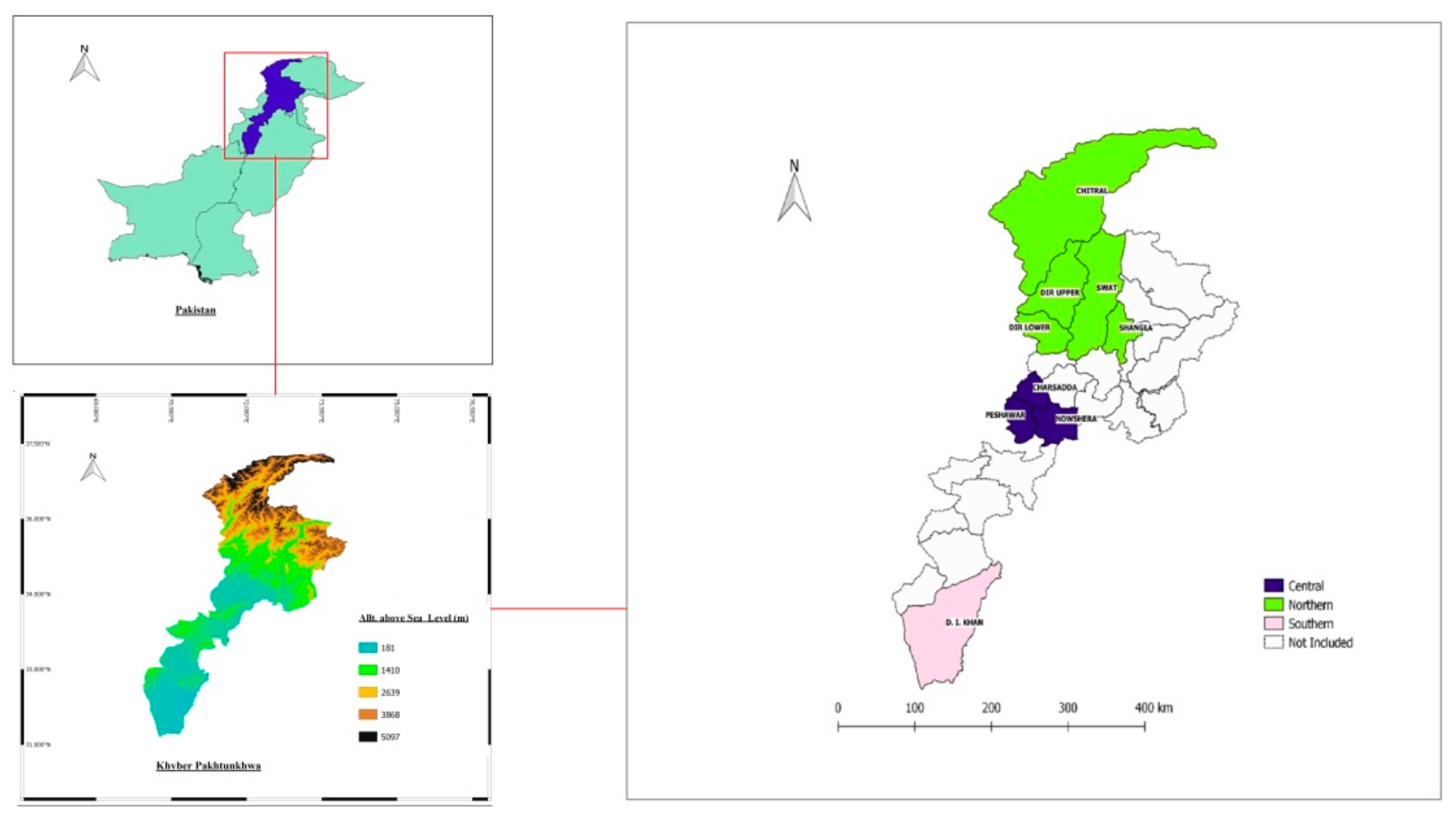
2.1. Study Area

The selected nine flood-prone districts of Khyber Pakhtunkhwa are the representatives of the three different geographical and climatic settings (Figure 1). These districts are selected based on the reports of the Provincial Disaster Management Authority and data set availability. The selected districts are;
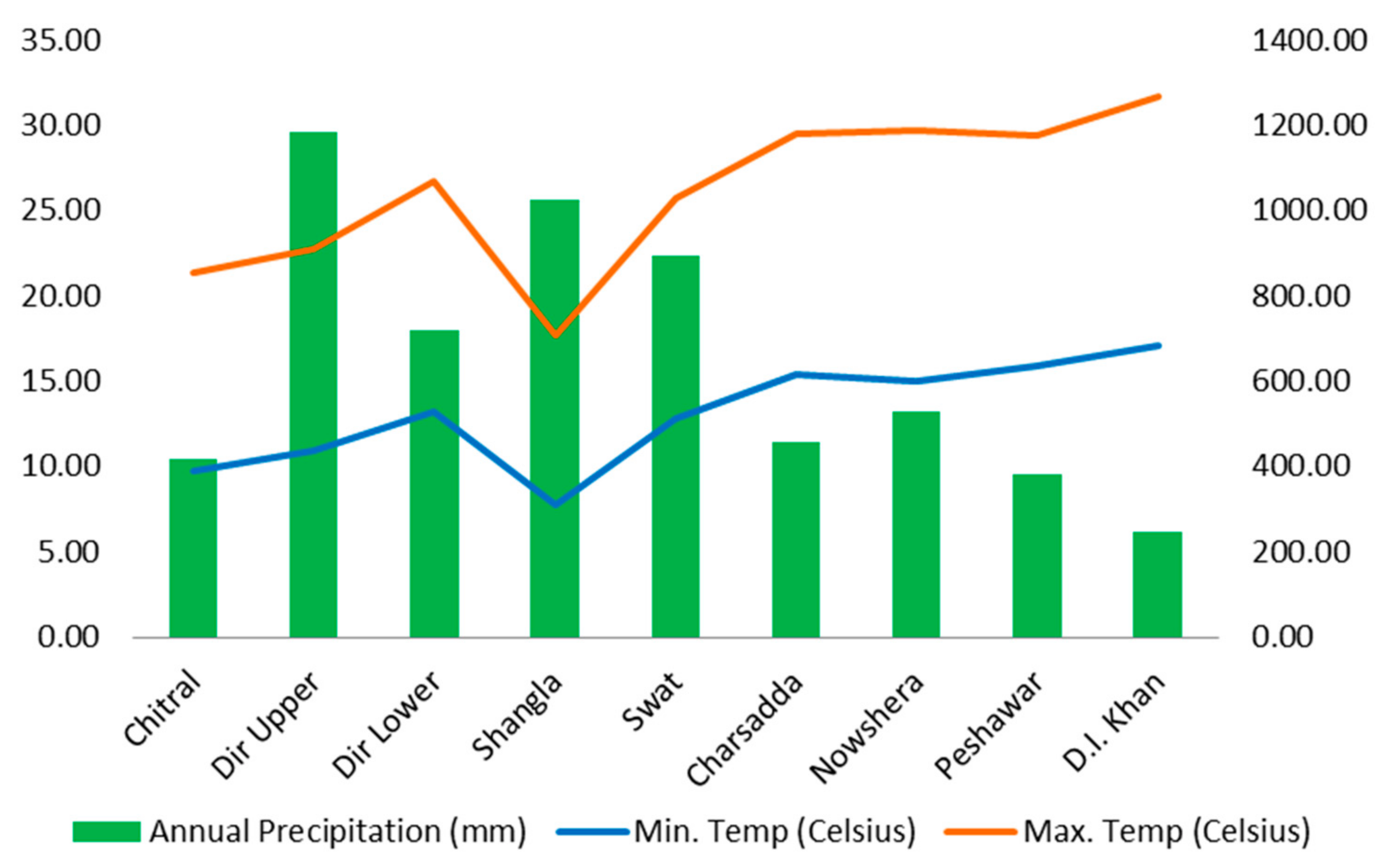
  • Chitral, Dir Upper, Dir Lower, Shangla, and Swat: Geographically they are situated in the upstream northern mountainous part of the province.
  • Charsadda, Nowshera, and Peshawar: Geographically they are in the downstream central plain part of the province.
  • D. I. Khan: Geographically it is also situated downstream in the southern plain part of the province.
The prevailing climatic conditions in terms of mean annual maximum temperature, mean annual minimum temperature, and the annual rainfall (1982–2012) in the selected districts are shown in Figure 2. It can be seen that as one moves from north (left) to south (right), temperature rises. While the annual precipitation, on the other hand, increases as one moves from south (right) to north (left), except for the extreme west, i.e., Chitral district. This variability in climatic parameters (temperature and precipitation) is due to the topographic variation and land physical features [14]. Furthermore, land physical features, such as forestry, are founded primarily in the province’s northern mountainous areas.

2.2. Construction of Flood Vulnerability Indices

The flood vulnerability assessment through indicators-based approach is conducted over a step-wise procedure [8,11,12] in following sub-sections.

2.2.1. Indicators Selection

The composite indicators can be built mainly by means of two different approaches known as inductive reasoning and deductive reasoning [26]. In a deductive approach, a theory or conceptual framework is used for the selection of indicators that best suit the relationship or phenomena to be measured. Simply put, it is the operationalization of a concept or testing hypothesis of the concept by gathering suitable data to explore the underlying relationship. While the inductive approach is based primarily on statistical and empirical generalizations [26]. We used deductive reasoning for the selection of preliminary set of indicators by employing the MOVE (Methods for the Improvement of Vulnerability Assessment in Europe) vulnerability assessment framework [27]. The framework conceptualized (flood) vulnerability as a product of three vulnerability factors included exposure, susceptibility and lack of resilience. The MOVE framework elaborated the three vulnerability factors, such as that exposure is “the extent to which an area that is subject to an assessment falls within the geographical range of a hazard event”. Similarly, susceptibility means “the predisposition of elements at risk (social and ecological) to suffering harm resulting from the levels of fragility of settlements, disadvantageous conditions and relative weaknesses” [27,28]). While lack of resilience is the “limitations in access to and mobilization of the resources of the human settlements and their institutions and the incapacity to adapt and respond in absorbing the socio-ecological and economic impact. The resilience includes the capacity to anticipate, cope and recover” [29].
The preliminary set of indicators is shown in Table 1. Literature shows that population density increases flood exposure [28,30,31,32]. As it is difficult for the dense population to evacuate easily and thus increase the potential to cause harm. The places where more people live in flood-prone areas tend to be highly exposed to flooding as compared to areas where relatively fewer people live in flood-prone areas [30,33]. Flood prone union councils (small administrative units) with respect to total union councils of a given district is used as a proxy indicator. Houses situated on low elevated areas are considered in high exposure category [28,34]. Altitude above sea level is used as proxy for this indicator. This indicator can best be used in local flood vulnerability where the relative height of the houses can be identified. There are, however, some reservations about this indicator. It is said that the flood can cause high damage in a flat area where the water can stay for a long time, and that high speed in a narrower valley can also cause high damage [2]. In the context of the study area, the central and southern districts are mainly plain, while the northern regions are mountainous. This will be checked against other indicators for the final list of indicators. Women are considered in the highly vulnerable category compared to the men because of less mobility, care, and income, which make it difficult to deal with and recover easily from disasters [23,28,35]. In regions where maternal mortality rates [36] or child mortality rates are higher [30], flood vulnerability is also higher by proposing a socio-economic disadvantaged area. The proportion of children to household members in an economically active age group is one of the limiting factors in satisfying daily household requirements (e.g., food), is a significant indicator [37] for flood vulnerability assessment. It is assumed that the larger the area dependency ratio, the more likely the higher the flood vulnerability. In terms of showing a socio-economically poor region, it is also believed that the lack of basic human requirements, such as access to improved drinking water and sanitation, will increase flood vulnerability by increasing the likelihood of epidemics and drinking water scarcity [38,39]. Literature also demonstrated that the unemployed are more likely to have problems with natural hazards and to recover from them [31,35,40,41]. Residential property effects the potential losses and recovery [23,35,42]. The greater proportion of Kacha houses in the area (where low-quality materials are used in house construction) indicates low resilience and higher vulnerability to flooding [43,44]. Agricultural land is used as a proxy for vulnerable occupations [23,43]. It has been observed that the potential for harm to agricultural land induced by heavy flooding is higher than its productivity, which is more likely to have an effect on agriculture-related people who use land as a source of food and income [43].
Literature has shown that education can improve comprehension, awareness, and resilience against flood disaster [41,42]. Whereas access to the lifeline reduces vulnerability [43,45,46]. The number of hospitals is used as proxy indicator in the current study. The indicator determines the capacity per district of public healthcare facilities. It has a significant impact on the ability of a region to deal with emergency response during disaster events [43]. The higher evacuation routes in terms of asphalt roads [30] imply the less complicated evacuation process [31], which can affect the vulnerability. Besides the function as a flood barrier to reduce the velocity of runoff and erosion [43], vegetation can act as a buffer zone for water decontamination [47]. Thus, the potential for harm to less forested areas will increase, implying that the community’s coping ability will greatly reduce (Ortwin 2006 in [43]). The forest area per district is calculated through the land utilization data with respect to overall reported area per district. Income enhance the capacity to cope and recover from a disaster easily [23,31,35]. It is mainly assumed that households with higher incomes or resources are less vulnerable than those with lower incomes or resources. Finally, it is also observed that flood management/protection measures in terms of structural interventions can reduce flood vulnerability [18,30]. The higher the region’s flood control measures, the less likely the vulnerability to flooding. The number of completed flood management projects are used as a proxy indicator. Note that indicators are resilience indicators in real sense that values are reversed to make it lack of resilience.
Table 1. Flood Vulnerability Indicators.
FactorsAbbreviation-Indicators (Unit)Data Source
ExposurePD—Population density (persons/ Km2)Calculated [48]
FPA—Flood prone area (%)Calculated [15]
AASL—Altitude Above Sea Level (m)[25]
SusceptibilityWMN—Women gender (%)Calculated [48]
MMR—Maternal mortality rate (per population)[49]
CMR—Child mortality rate (per 1000 live birth)[49]
DPR—Dependency ratio (%)[37]
LAIW—Lack of access to improved drinking water (%)[37]
LAIS—Lack of access to improved sanitation (%)[37]
UNE—Unemployment (%)Calculated [50]
KH—Kacha houses (%)[37]
AGL—Agricultural land (%)[50]
Lack of ResilienceLR—Literacy rate (%)[50]
NH—Numbers of hospitals (per districts)[50]
ASR—Length of asphalt roads (km/km2)[51]
FC—Forest cover (%)Calculated [50]
MMHI—Mean monthly household income (US$)[37]
FMM—Flood management measures (number)[52]
Calculated: Calculated from the source given in bracket.

2.2.2. Data Treatment

There are several steps to treat data for missing values, outliers, and double counting or redundancy. Missing some indicators or data of some regions are not uncommon in the development of composite indicators. In this regard, different options for the substitution of missing data exist [8]. However, we did not face this problem in the current study. Rules also exist for the detection of outliers, such as the combined use of skewness and kurtosis [53]. Though, some authors said that it will change the actual data structure that can creates hurdles in interpretation, and can suppress the presence of extreme values [11]. Therefore, we did not treat the data for this issue. The question of double counting of the indicators is another important step to be considered in the formation of composite indicators. Indicators reduction (based on correlation) is actually a very big dilemma in the development of composite indicators. There will always be positive correlation among indicators [8], while Saisana & Tarantola (2002 in [54]) opined that completely independent indicators cannot be selected if they measure the same phenomena. Though it is desired to use independent indicators, still some authors considered this issue as “unrealistic” [8]. However, different views exist for the selection of certain indicators when they are highly correlated. It is generally accepted that if the two or more indicators representing the same phenomena and there is a high correlation, then it is necessary to discard certain indicators using a “rule of thumb”. For instance, if two indicators are logically correlated, then the rule is applicable, but if the correlated indicators represent different phenomena, then the rule can be safely neglected (see [11]). The cut-off value of Pearson’s correlation (r) for strong linear relationship as a “rule of thumb” was reported differently in different studies, such as 0.65 [11], 0.70 [30], and 0.90 [55]. We used 0.65 [11] in this study. Where original indicators are not accessible, proxy indicators can be used [7]. Commensurability is also required in case of comparison across the administrative units to bring indicators into comparable unit [7]. For instance, if Region A has 40,000 women and Region B has 20,000, the comparison will be misleading, as one does not know the proportion of women with respect to overall population. The conversion of these values into percentages with respect to the total population in a given district can therefore ensure reliable results.

2.2.3. Data Rescaling

To avoid the adding up “apples and oranges” the data need to be transformed into a single scale [8]. Several methods exist for this purpose; however, when selecting the appropriate method, the data properties and objectives of the composite indicator should be taken into account by practitioners [53]. Though, it was reported that deductive and hierarchical designs generally apply “Min-Max” normalization (min-max linear scaling) to convert values to a min-max scale (such as 0 to 1), whereas indices that use inductive designs tend to apply a z-score normalization technique that generates variables with a mean of zero and a standard deviation of one [7]. However, several studies used it for both reasoning (see [11]). Therefore, we used both approaches in the current study.
Indicators that have a direct relationship with vulnerability are rescaled through Equation (1). While the indicators that have inverse relationship with vulnerability were rescaled through Equation (2) [12,28,56,57,58];
X i = X a X M i n X M a x X M i n
X i = X M a x X a X M a x X M i n
where Xi means the normalized value, Xa is the actual value, XMax is the maximum value, and XMin is the minimum value for an indicator i, across the selected districts.
In the second method, the mean is subtracted from the actual value and divided by the standard deviation of an indicator across the selected districts, as given in Equation (3) [8,11];
X i = X a X ¯ σ
where X ¯ stands for mean values, and σ for standard deviations. Note that the lack of resilience indicators was reversed in this case before data rescaling.

2.2.4. Weighting

Weights can have a substantial effect on the overall composite indicator [8]. Weights to indicators may be equal or differential. Equal weights are used in these cases, if there is insufficient understanding of causal relationships or a lack of consensus on the alternative weighting schemes. Equal weights and “no weights” are often used in synonym [7,8]. So, we did not apply any weights to indicators as in the study of Villordon [34]. Note that indicators will get equal weights only with respect to sub-indices. Whereas, when weights are decided to be unequal or differential, three ways that are normative, data-driven, and hybrid are usually adapted (Decancq & Lugo 2013 in [7]). Normative approach consists on expert opinion, public opinion, or stakeholders’ consultation, while data-driven means the weights are derived through some statistical or empirical means like principal component analysis (PCA), factor analysis, regression etc. [7,8,53]. However, statistical methods are sometimes considered to be more scientifically defensible and less resource-intensive [59]. We used statistically derived differential weights in the current study.
The first approach used in the current study is known as the Iyenger and Sudarshan’s method (IS) [56]. In this approach, the weights are assumed to vary inversely as the variance over the regions in the respective indicators of vulnerability [28,58]. It is also reported that calculating weights through this approach “would ensure that large variation in any one of the indicators would not unduly dominate the contribution of the rest of the indicators and distort inter-regional comparisons” [32,58]. The weights for each indicator i across the selected districts are calculated through Equation (4);
W i = K V a r   X i
where Wi ( i = 1 n W i = 1 and 0   W i 1 ) is the weights for n number of indicators, and K is the normalized constant that is calculated using Equation (5);
K = i = 1 n 1 V a r   X i 1
The second weighting scheme adopted in the current study is based on principal components analysis (PCA). Varimax rotation with eigenvalue greater than 1 approach (Kaiser Criterion) is applied [10]. The weights are calculated using Equation (6) (Nicoletti et al., 2000 in [8,11]);
W i = F L 2 T V R S L
where, FL implies the factor loading and TVRSL for total variance of the rotated square loadings.

2.2.5. Aggregation

The commonly used aggregation options are summation (linear aggregation), multiplication (geometric aggregation), and multicriteria analysis. The most common technique for calculating the overall index is a simple averaging method [59]. Compensability can be a weakness of additive aggregation if a low value in one indicator or dimension masks a high value in another (Tate 2012 in [7]). So, we also used a partially non-compensable (multiplicative) aggregation in this study.
The non-weighted normalized indicators are aggregated through Equation (7) for factor-wise sub-indices (Booysen (2002) and Tate (2012) in [60]) using additive function;
S I = i = 1 n X i n
While Equation (8) is used for the multiplicative aggregation (geomean) of sub-indices (Nardo et al., 2005 in [60]). One was added to all indicators as multiplicative function is strictly applicable in positive data [61].
S I = i = 1 n X i 1 n
where, SI stands for sub-indices exposure (SIE), susceptibility (SIS), and lack of resilience (SILoR) for n numbers of indicators in each factor.
The weighted normalized indicators are aggregated into its respective flood vulnerability factors using Equation (9) [8,28,58,59,60,62];
S I = i = 1 n W i X i
The overall flood vulnerability index values for the selected districts are calculated through Equation (10) using additive function, while Equation (11) as multiplicative function ([62]);
F V I = 1 3 S I E + S I S + S L o R
F V I = S I E × S I S × S I L o R 1 / 3

2.2.6. Robustness Check

Robustness test (uncertainty and sensitivity analysis) is related with “X-ray” of the underlying phenomena, i.e., the checking of assumptions made during the development of composite indicators [8]. Literature shows that the methodological choices made during the various stages of the composite index construction involve assumptions, subjectivity, and uncertainties that should be identified, acknowledged, and communicated across the quantitative procedure [7]. It is also referred as robustness tests in terms of uncertainty and sensitivity analysis. It is often seen that these two are handled independently, with uncertainty analysis being the most common type of robustness check. The analysis of uncertainty refers to variations observed in the final results (i.e., the composite index value) from a possibly different choice made in the inputs (i.e., the composite index stages). Whereas sensitivity analysis estimates how much variability of the overall output is attributed to these uncertainties [9]. Different views exist in the scientific community about the use of robustness tests. The assessment of uncertainty and sensitivity is not optional, but essential to guarantee transparency of the vulnerability assessment indices. However, the use of highly sophisticated approaches that gets dominant over logical cohesion are also not desirable [7]. There are different techniques that can be used for robustness tests, such as correlation analysis [60] and volatility tests using standard deviations [11]. However, the “average shift in ranking, ( R ¯ s )” [8,12,54] in comparisons to a reference is the easier one. Hudrliková’s approach [12] is adopted here to know the relative ranking of flood vulnerability of the selected districts with respect to different methodological approaches using Median ranking (MR) as a reference. The lower value near to zero will indicate the more similar ranking to median ranking. It was reported that median ranking is perceived to be the most accurate ranking in comparison to other approaches that are largely influenced by data issues, such as highly correlated indicators, presence of extreme values, etc. [12]. Spearman correlation is also used for such purposes [60]. The higher correlation coefficient between the MR and other methodological approaches will indicate the most similar and stable ranking. An open source software [63] was used for statistical analysis.
The current study constructed flood vulnerability composite indicators through five different approaches, as shown in Table 2. The first model (MMNA) is the simplest one that is frequently used in the scientific community, where the normalized indicators are simply averaged through additive function. Here “MM” means that the indicators are normalized through “min-max” method, “N” means that “no” weights are assigned to indicators, and “A” imply that the aggregation is based on “additive” function. This is the base model, where we have assumed that its construction, interpretation, and comprehension are extremely simple. Similarly, MMISA implies that the indicators are normalized through the min-max approach, the weights are allocated to indicators through Iyenger and Sudarshan’s method, and additive function is used for aggregation; MMPCA means that almost similar approach is used for data rescaling and aggregation, except for weights that are extracted through PCA approach; ZSNA means that the indicators are rescaled through the Z-score approach, where no weights are applied and aggregated through additive function, and MMNG means that indicators are normalized through min-max approach with no weights to indicators that are aggregated through multiplicative function.

3. Results

Before proceeding to final indicators selection, commensurability was confirmed. It was simply developed by transforming the datasets into percentages (if given in different units or not comparable in given form) for the districts concerned. Data were processed using the Pearson correlation matrix to know highly correlated indicators (see Table A1 in Appendix A). It was noticed that some indicators were highly correlated with others that were based entirely on general understanding. DPR, WMN, LAIW, and CMR were found to be highly correlated. Intuitively, all these are linked to one another, so the DPR is retained, while the remaining three are discarded as a DPR in some sense more attributed to all these indicators. UNE was found to be highly correlated with KH, as individuals with constant sources of income are usually assumed to live in decent houses. It was thus excluded from the final list of indicators. NH is also found to be highly correlated with PD, which means that health facilities are provided on a population-based principle. It was therefore discarded from the final list of indicators. AASL was found to be highly correlated with a number of indicators such as LAIW, UNE, FC, and FMM. If the socio-economic relationship is ignored such that unemployment in mountainous areas is higher than in plain areas, it cannot be ignored that forests are primarily found in mountainous districts of the province. So, it was discarded from final list of indicators. It will also generate confusion if plain areas are deemed highly vulnerable compared to mountainous areas or vice versa, because flood damage depends on the type of flood hazard. For final flood vulnerability assessment, twelve indicators are retained with clear policy implications (Appendix A, Table A2). Although data is skewed, no further data is treated before normalization, as it will change the original data structure. The weights that get by each indicator through differential weighting approaches are shown in Table 3 and Table 4, respectively. The weights that get by each indicator through PCA approach are highlighted in bold.
The comparative ranking of flood vulnerability for the selected districts of Khyber Pakhtunkhwa, derived through different methodological approaches is shown in Table 5. The robustness tests were done by comparing the ranks that are derived through different methods, with median ranks using average shift in rank (approach (Table 6). No change in ranking is observed with respect to data rescaling. With respect to aggregation, a very nominal shift in rank (0.22) is observed. Interestingly, empirical weights that are derived through PCA as well as IS methods showed similar values (1.56).
These findings are also demonstrated through the correlation coefficients that ranged from 0.80 to 1.00 between median ranking and the other methodological approaches (Table 7).
To know this variability in ranking due to a slightly higher R ¯ s and lower Spearman rho of weighted and aggregation approaches, all the derived ranking through different approaches (representing by line) were plotted against median ranking (representing by triangle mark) in ascending order (Figure 3). The results indicate that a maximum of two degrees shift in ranking can be seen in Charsadda, Dir Upper, Swat, Chitral, and D.I. Khan due to differential weights. While not using these weighted methods, only two districts (Dir Upper and Swat) can shift their ranks up to one degree due to multiplicative aggregation, as shown in Figure 4. These results imply that the weights have substantial influence on the overall flood vulnerability indices in the context of current study as compared to data rescaling and aggregation through multiplicative method. The perfect matching of MMNA with ZSNA ( R ¯ s = 0.00, Spearman rho = 1.00) and MMNG (( R ¯ s = 0.22, Spearman rho = 0.98) indicates that the flood vulnerability indices derived through these approaches will not largely affect the overall ranking of the selected districts. These results imply that the base model can be used for further investigation while disintegrating it into its sub-indices and indicators for the selected districts (that are coming in our next papers).

4. Discussion

Thorough knowledge of the most vulnerable regions, populations, and key drivers that actually create such vulnerability is an effective tool for disaster risk reduction, reconstruction strategies, and policy making [21]. Vulnerability assessment research in general and flood vulnerability assessment research in particular are very raw within this part of the world. As the flood risk management is the collective activity of several experts such as hydrologists, hydraulic engineers, economists, social scientists, ecologists, and planners to reduce flood risks [3], therefore, the objective of this study is to make the flood vulnerability assessment approach not only comprehensible to a wide range of stakeholders, but also scientifically defensible.
The construction of (vulnerability) composite indicators has several challenges. It is reported that there is not a single universally accepted method that can be used to construct composite indicators [64]. It has been observed that analytic versus pragmatic issues are the top most issue of controversy between aggregators (who favor composite indicators) and non-aggregators (who are against composite indicators) [53]. It is also held that the techniques for developing aggregate or composite vulnerability indices (using deductive approach) are not technically complicated, though they can be highly contentious due to a number of subjective and intrinsic assumptions that need to be made [59]. Booysen (2000 in [9]) states that this is logical, because there are many phases in the development of composite indicators, and at the same time criticism could grow for each of them. Each step of the composite indicator is “between the devil and deep blue sea” that can compel the developer to make compromises in each step [9]. Even the well-known indices are not exempted from analytic problems [8]. Mainly, the indicators rescaling, weighting, and aggregation through inductive and deductive reasoning can significantly influence the composite indicators for vulnerability assessment [8,11,12,65]. Apparently, there is no single best data rescaling, weighting, and aggregation method, as final composite indicators are mainly data specific for each study [60]. The current study contributes to address this important issue by selecting a more robust approach to flood vulnerability by building a consensus among stakeholders to overcome the subjectivity issue.
In the current study, we only covered the methodological issues to construct flood vulnerability indices. The study facilitates to select the appropriate approach in the context of current study. Through the findings of this study, the policy-makers can get a vivid picture of the overall flood vulnerability across the selected districts that will help them to get valuable information for robust decision making to reduce flood risk and to expand the approach for the remaining districts. Note that the results are for large scale that are not able to discriminate heterogeneity within the districts, therefore, the results area generalized form of flood vulnerability that can be viewed as average [24] or homogeneous flood vulnerability [66]. That means to identify homogenous regions in terms of their degree of vulnerability as well as their inherent characteristic [66], which can be used as an evidence to highlight vulnerable areas for further investigation [67].
It is also to be noted that, there are always some issues related to vulnerability indices. As there are always limitations in these types of studies, since these sorts of studies are based primarily on assumptions that best fit the phenomena to be measured. Such studies are the simplification of a complex real system [11,54], and it is difficult to validate its results [67]. The indices of vulnerability are still regarded as “reified snapshot” [68]. Though, (flood) vulnerability is a dynamic process which is less likely to remain constant [69], still the indices can serve as a proxy for identifying ways to increase resilience [67]. It is also reported that the measures that can reduce the losses from one hazard are not separate from other hazards in many cases [70]. So, the results of the current study can be used as a benchmark for the subsequent studies. There are several unsolved issues with respect to application of flood vulnerability composite indicators such as the inability to show the exact extent of expected damages, data time span, etc. (for detail [68]). We left this issue for other researchers.
These limitations leave room for further studies. Since each model is the simplification of a complex real system, and only those factors can be operationalized as far as the (official) data allowed. However, due to its open structure, further indicators can be accommodated, or the composite indicators can be updated [54]. Although it is reported that the debate will never be settled in the development of composite indicators among varying stakeholders (Saisana et al., 2005 in [8]), there is still room for improvement. Opening up the entire construction process to all stakeholders and the general masses is the basis for its reliability and transparency [7,8], that we have demonstrated in this study. So, the approach employed in this study is relatively easy from an interdisciplinary point of view, where flexibility is made to construct flood vulnerability indices without involving highly sophisticated empirical approaches for a wide range of stakeholders. Even though there’s too much criticism of the use of the composite indicator, the irresistible nature of the composite indicator for policy intervention is still difficult to resist [9].

5. Conclusions

Selecting the most appropriate approach for the development of composite indicators for flood vulnerability assessment is a challenging task due to its data-specific nature for each study, especially in the realm where multiple stakeholders are involved, and where there is a possibility of subjectivity. We have demonstrated to solve these important issues in the context of Khyber Pakhtunkhwa, by making the flood vulnerability composite indicators using various methodological approaches with a fairly simple robustness approach. The basic model was found to be robust compared to other selected approaches that could be used for further investigation for the current dataset. These findings can also suggest that a simple method for the development of flood vulnerability indices is a good approach, keeping in mind the interdisciplinary nature of flood risk management. However, to ensure its robustness, it needs to be cross-checked with other methodological approaches, and to make them scientifically defensible in a simple and easy way to understand. The study provides decision-makers and concerned authorities with a meaningful tool to identify and prioritize certain vulnerable areas and actions to reduce the existing flood vulnerabilities while planning for future flood risk reduction in the province through a methodologically defensive way. The study also provides a baseline or benchmark for assessing the efficiency of flood risk reduction interventions over time where the future studies can be related. To get the full image of the flood risk in the selected districts, hazard assessment is as important as the vulnerability assessment. The methodology used in the current study can also be used in different parts of the world to address flood vulnerability or even social vulnerability using different composite indicators’ building approaches.

Author Contributions

Muhammad Nazeer has conceptualized and written the article while Hans-Rudolf Bork has critically revised the manuscript draft.

Funding

This research received no external funding.

Acknowledgments

We acknowledge financial support by Land Schleswig-Holstein (Germany) within the funding program Open Access “Publikationsfonds”. We also extended our gratitude for the valuable feedback from the anonymous reviewers in the improvements of this manuscript.

Conflicts of Interest

The authors declare no conflict of interest.

Appendix A

Table A1. Correlation Analysis.
PDFPAAASLWMNCMRMMRDPRLAIWLAISKHAGLUNELRASRFCMMHIFMMNH
PD1.00−0.07−0.48−0.370.200.17−0.41−0.68−0.21−0.600.36−0.490.480.57−0.510.420.760.81
FPA−0.071.000.14−0.400.48−0.39−0.32−0.32−0.21−0.52−0.55−0.16−0.46−0.08−0.33−0.320.24−0.30
AASL−0.480.141.000.48−0.400.340.550.66−0.230.460.010.70−0.49−0.480.71−0.39−0.66−0.30
WMN−0.37−0.400.481.00−0.760.340.950.550.010.590.440.39−0.210.170.91−0.04−0.37−0.27
CMR0.200.48−0.40−0.761.00−0.18−0.83−0.57−0.02−0.50−0.37−0.530.13−0.10−0.700.410.390.09
MMR0.17−0.390.340.34−0.181.000.390.410.360.230.280.17−0.20−0.230.400.54−0.080.56
DPR−0.41−0.320.550.95−0.830.391.000.700.170.520.220.40−0.420.060.90−0.18−0.41−0.22
LAIW−0.68−0.320.660.55−0.570.410.701.000.430.68−0.150.55−0.56−0.510.70−0.33−0.82−0.30
LAIS−0.21−0.21−0.230.01−0.020.360.170.431.000.22−0.26−0.13−0.52−0.18−0.090.13−0.150.04
KH−0.60−0.520.460.59−0.500.230.520.680.221.000.430.73−0.19−0.360.58−0.20−0.86−0.48
AGL0.36−0.550.010.44−0.370.280.22−0.15−0.260.431.000.310.430.350.230.27−0.010.19
UNE−0.49−0.160.700.39−0.530.170.400.55−0.130.730.311.00−0.21−0.610.51−0.46−0.74−0.34
LR0.48−0.46−0.49−0.210.13−0.20−0.42−0.56−0.52−0.190.43−0.211.000.30−0.240.400.380.39
ASR0.57−0.08−0.480.17−0.10−0.230.06−0.51−0.18−0.360.35−0.610.301.00−0.150.160.590.18
FC−0.51−0.330.710.91−0.700.400.900.70−0.090.580.230.51−0.24−0.151.00−0.09−0.53−0.26
MMHI0.42−0.32−0.39−0.040.410.54−0.18−0.330.13−0.200.27−0.460.400.16−0.091.000.500.58
FMM0.760.24−0.66−0.370.39−0.08−0.41−0.82−0.15−0.86−0.01−0.740.380.59−0.530.501.000.59
NH0.81−0.30−0.30−0.270.090.56−0.22−0.300.04−0.480.19−0.340.390.18−0.260.580.591.00
Table A2. Final List of Indicators.
DistrictsPDFPADPRMMRLAISKHAGLLRASRFCMMHIFMM
Charsadda1622.6948.9899.8830.0021.9775.0092.2044.000.410.001.255.00
Chitral30.1320.83103.00128.002.2591.6084.7055.000.1042.971.250.00
D.I. Khan222.1025.5398.32124.0050.9476.1042.4041.000.160.541.252.00
Dir Lower907.0918.92118.7593.0014.5671.5072.7049.000.4754.341.254.00
Dir Upper255.8617.86120.52557.0042.2391.6083.6036.000.2064.291.752.00
Nowshera868.7357.1490.8474.0015.4557.7051.2050.000.305.121.756.00
Peshawar3396.2426.0994.22375.0016.8151.6080.1056.000.330.081.758.00
Shangla477.8167.86106.52226.0018.6271.7049.2030.000.1832.311.001.00
Swat432.7569.23106.20103.0019.3755.3043.0039.000.1927.301.256.00

References

  1. Balica, S.F. Approaches of Understanding Developments of Vulnerability Indices for Natural Disasters. J. Environ. Eng. 2012, 11, 1–12. [Google Scholar] [CrossRef]
  2. Kron, W. Flood Risk—A Global Problem; ICHE: Hamburg, Germany, 2014; pp. 9–18. [Google Scholar]
  3. Nasiri, H.M.; Yusof, J.M.; Ali, T.M.A. An Overview to Flood Vulnerability Assessment Methods. Sustain. Water Res. Manag. 2016, 2, 331–336. [Google Scholar] [CrossRef]
  4. Ciurean, R.L.; Schröter, D.; Glade, T. Conceptual Frameworks of Vulnerability Assessments for Natural Disasters Reduction. In Approaches to Disaster Management: Examining the Implications of Hazards, Emergencies and Disasters; Tiefenbacher, J., Ed.; InTech: London, UK, 2013; pp. 3–32. [Google Scholar] [CrossRef]
  5. Fussel, H.M. Vulnerability: A Generally Applicable Conceptual Framework for Climatic Research. Glob. Environ. Chang. 2007, 17, 155–167. [Google Scholar] [CrossRef]
  6. Brooks, N. Vulnerability, Risk and Adaptation: A Conceptual Framework; University of East Anglia, Tyndall Centre for Climate Change Research: Norwich, UK, 2003. [Google Scholar]
  7. Baptista, S.R. Design and use of Composite Indices in Assessment of Climate Change Vulnerability and Resilience; Tetra Tech ARD: California, CA, USA, 2014. [Google Scholar]
  8. Organization for Economic Co-operation and Development. Handbook on Constructing Composite Indicators: Methodology and User Guide; Organization for Economic Co-operation and Development: Paris, France, 2008. [Google Scholar]
  9. Greco, S.; Ishizaka, A.; Tasiou, M.; Torrisi, G. On the Methodological Framework of Composite Indices: A Review of the Issues of Weighting, Aggregation, and Robustness. Soc. Indic. Res. 2019, 141, 61–94. [Google Scholar] [CrossRef]
  10. Roder, G.; Sofia, G.; Wu, Z.; Tarolli, P. Assessment of Social Vulnerability to Floods in the Floodplain of Northern Italy. Weather Clim. Soc. 2017, 9, 717–737. [Google Scholar] [CrossRef]
  11. Damm, M. Mapping Social-Ecological Vulnerability to Flooding—A sub-national approach for Germany. Master’s Thesis, Rheinischen Friedrich-Wilhelms-Universität, Bonn, Germany, 2010. [Google Scholar]
  12. Hudrliková, L. Composite Indicators as a Useful Tool for International Comparison: The Europe 2020 Example. Prague Eco. Pap. 2013, 22, 459–473. [Google Scholar] [CrossRef]
  13. Etter, J.; Hidajat, R.; Müller, C.; Velte, B. Linkages for Effective Disaster Management in Khyber Pakhtunkhwa Province; GTZ: Islamabad, Pakistan, 2011. [Google Scholar]
  14. Rahman, A.-u.; Khan, A.N. Analysis of 2010-Flood Causes, Nature and Magnitude in the Khyber Pakhtunkhwa, Pakistan. Nat. Hazards 2013, 66, 887–904. [Google Scholar] [CrossRef]
  15. Monsoon Contingency Plan 2017. Available online: https://www.pdma.gov.pk/sites/default/files/MCP%202017.pdf (accessed on 6 June 2018).
  16. Environmental Protection Agency. Khyber Pakhtunkhwa Climate Change Policy; Environmental Protection Agency, Government of Khyber Pakhtunkhwa Forestry, Environment & Wildlife Department: Peshawar, Pakistan, 2016. [Google Scholar]
  17. Akhter, M.I.; Irfan, M.; Shahzad, N.; Ullah, R. Community Based Flood Risk Reduction: A Study of 2010 Floods in Pakistan. Am. J. Soc. Sci. Res. 2017, 3, 35–42. [Google Scholar]
  18. Qasim, S.; Khan, A.N.; Shrestha, R.P.; Qasim, M. Risk Perception of the People in the Flood Prone Khyber Pukhthunkhwa Province of Pakistan. Inter. J. Disaster Risk Red. 2015, 14, 373–378. [Google Scholar] [CrossRef]
  19. Aslam, M.K. Agricultural Development in Khyber Pakhtunkhwa: Prospects, Challenges and Policy Options. Pak. A J. Pak. Stud. 2015, 4, 49–68. [Google Scholar]
  20. Khan, A.N.; Khan, S.N.; Safi Ullah, A.M.; Qasim, S. Flood Vulnerability Assessment in Union Council Jahangira, District Nowshera, Pakistan. J. Sci. Tech. Univ. Peshawar 2016, 40, 23–32. [Google Scholar]
  21. Birkmann, J. Risk and Vulnerability Indicators at different Scales: Applicability, Usefulness and Policy Implications. Environ. Hazards 2007, 7, 20–31. [Google Scholar] [CrossRef]
  22. Cutter, S.L.; Mitchell, J.T.; Scott, M.S. Revealing the Vulnerability of People and Places: A Case Study of Georgetown County, South Carolina. Ann. Am. Assoc. Geogr. 2000, 90, 713–737. [Google Scholar] [CrossRef]
  23. Cutter, S.L.; Boruff, B.J.; Shirley, W.L. Social Vulnerability to Environmental Hazards. Soc. Sci. Q. 2003, 84, 242–261. [Google Scholar] [CrossRef]
  24. Fekete, A. Assessment of Social Vulnerability for River-Floods. Ph.D. Thesis, United Nations University—Institute for Environment and Human Security, Bonn, Germany, 2010. [Google Scholar]
  25. Climate-Data.org. (n.d.). Available online: https://en.climate-data.org/ (accessed on 27 July 2018).
  26. Adger, W.N.; Brooks, N.; Bentham, G.; Agnew, M.; Eriksen, S. New Indicators of Vulnerability and Adaptive Capacity; Tyndall Centre for Climate Change Research Norwich: Norwich, UK, 2004. [Google Scholar]
  27. Birkmann, J.; Cardona, O.D.; Carreno, M.L.; Barbat, A.H.; Pelling, M.; Schneiderbauer, S.; Welle, T. Framing Vulnerability, Risk and Societal Responses: The MOVE Framework. Nat. Hazards 2013, 2, 193–211. [Google Scholar] [CrossRef]
  28. Kablan, M.K.; Dongo, K.; Coulibaly, M. Assessment of Social Vulnerability to Flood in Urban Côte d’Ivoire Using the MOVE Framework. Water 2017, 9, 292. [Google Scholar] [CrossRef]
  29. CORDIS. Methods for the Improvement of Vulnerability Assessment in Europe. Available online: https://cordis.europa.eu/project/rcn/88645/reporting/en (accessed on 2 August 2019).
  30. Balica, S.; Wright, N.G. Reducing the Complexity of the Flood Vulnerability Index. Env. Hazards 2010, 9, 321–339. [Google Scholar] [CrossRef]
  31. Holand, I.S.; Lujala, P.; Röd, J.K. Social Vulnerability Assessment for Norway: A Quantitative Approach. Nor. Geogr. Tidsskr. Nor. J. Geogr. 2011, 65, 1–17. [Google Scholar] [CrossRef]
  32. Hiremath, D.; Shiyani, R.L. Analysis of Vulnerability Indices in Various Agro-Climatic Zones of Gujarat. Indian J. Agric. Econ. 2013, 68, 122–137. [Google Scholar]
  33. Messner, F.; Meyer, V. Flood Damage, Vulnerability and Risk Perception—Challenges for Flood Damage Research; UFZ–Umwelt Forschungs Zentrum: Leipzig, Germany, 2005. [Google Scholar]
  34. Villordon, M.B. Community-Based Flood Vulnerability Index for Urban Flooding: Understanding Social Vulnerabilities and Risks; Université Nice Sophia Antipolis: Nice, France, 2014. [Google Scholar]
  35. Dwyer, A.; Zoppou, C.; Mielsen, O.; Day, S.; Roberts, S. Quantifying Social Vulnerability: A methodology for Identifying Those at Risk to Natural Hazards; Geoscience Australia: Canberra, Australia, 2004. [Google Scholar]
  36. Goodman, A. In the Aftermath of Disasters: The Impact on Women’s Health. Crit. Care Obstet. Gynecol. 2016, 2, 1–5. [Google Scholar] [CrossRef]
  37. Food Insecurity in Pakistan 2009. Available online: https://documents.wfp.org/stellent/groups/public/documents/ena/wfp225636.pdf (accessed on 3 March 2019).
  38. McCluskey, J. Water Supply, Health and Vulnerability in Floods. Waterlines 2001, 19, 14–17. [Google Scholar] [CrossRef]
  39. See, K.L.; Nayan, N.; Rahaman, Z.A. Flood Disaster Water Supply: A Review of Issues and Challenges in Malaysia. Int. J. Acad. Res. Bus. Soc. Sci. 2017, 7, 525–532. [Google Scholar] [CrossRef]
  40. Cutter, S.L.; Barnes, L.; Berry, M.; Burton, C.; Evans, E.; Tate, E.; Webb, J. A Place-based Model for Understanding Community Resilience to Natural Disasters. Glob. Env. Chang. 2008, 14, 598–606. [Google Scholar] [CrossRef]
  41. Kuhlicke, C.; Scolobig, A.; Tapsell, S.; Steinführer, A.; De Marchi, B. Contextualizing Social Vulnerability: Findings from Case Studies across Europe. Nat. Hazards 2011, 58, 789–810. [Google Scholar] [CrossRef]
  42. Muller, A.; Reiter, J.; Weiland, U. Assessment of Urban Vulnerability towards Floods using an Indicator-based Approach—A Case Study for Santiago de Chile. Nat. Hazards Earth Syst. Sci. 2011, 7, 2107–2123. [Google Scholar] [CrossRef]
  43. Rafiq, L.; Blaschke, T. Disaster risk and vulnerability in Pakistan at a district level. Geomat. Nat. Hazards Risk 2012, 3, 324–341. [Google Scholar] [CrossRef]
  44. Shah, A.; Khan, H.; Qazi, E. Damage Assessment of Flood Affected Mud Houses in Pakistan. J. Himal. Earth Sci. 2013, 46, 99–110. [Google Scholar]
  45. Jonkman, S.N.; Kelman, I. An Analysis of the Causes and Circumstances of Flood Disaster Deaths. Disasters 2005, 29, 75–97. [Google Scholar] [CrossRef]
  46. Jonkman, S.N.; Maaskant, B.; Boyd, E.; Levitan, M.L. Loss of Life Caused by the Flooding of New Orleans After Hurricane Katrina: Analysis of the Relationship Between Flood Characteristics and Mortality. Risk Anal. 2009, 29, 676–698. [Google Scholar] [CrossRef]
  47. Zanetti, C.; Macia, J.; Liency, N.; Vennetier, M.; Mériaux, P.; Provansal, M. Roles of the Riparian Vegetation: The Antagonism between Flooding Risk and the Protection of Environments. FLOODrisk—3rd European Conference on Flood Risk Management. E3S Web Conf. 2016, 7, 1–6. [Google Scholar] [CrossRef]
  48. Pakistan Bureau of Statistics. Available online: http://www.pbs.gov.pk/sites/default/files//DISTRICT_WISE_CENSUS_RESULTS_CENSUS_2017.pdf (accessed on 27 April 2018).
  49. Districts Health Information System. ANNUAL REPORT 2017. Available online: http://www.dhiskp.gov.pk/reports/Annual%20Report%202017%20N.pdf (accessed on 19 December 2018).
  50. Developmental Statistics of Khyber-Pakhtunkhwa 2017. Available online: http://www.pndkp.gov.pk/wp-content/uploads/2017/07/DEVELOPMENT-STATISTICS-OF-KHYBER-PAKHTUNKHWA-2017.pdf (accessed on 27 March 2018).
  51. Khyber Pakhtunkhwa’s Bureau of Statistics. Socio-economic Indicators of Khyber-Pakhtunkhwa. Peshawar, Pakistan: Government of Khyber-Pakhtunkhwa. 2017. Available online: https://kpbos.gov.pk/allpublication/2 (accessed on 10 June 2018).
  52. Irrigation Department of Khyber Pakhtunkhwa. Contingency Plan for Monsoon Season. Peshawar 2017. Available online: https://www.pdma.gov.pk/sites/default/files/MCP%202017.pdf (accessed on 26 November 2019).
  53. Saisana, M.; Saltelli, A. Rankings and Ratings: Instructions for Use. Hague J. Rule Law 2011, 3, 247–268. [Google Scholar] [CrossRef]
  54. Merz, M.; Hiete, M.; Comes, T.; Schultmann, F. A composite indicator model to assess natural disaster risks in industry on a spatial level. J. Risk Res. 2013, 16, 1077–1099. [Google Scholar] [CrossRef]
  55. Hagenlocher, M.; Hölbling, D.; Kienberger, S.; Vanhuysse, S.; Zeil, P. Spatial Assessment of Social Vulnerability in the Context of Landmines and Explosive Remnants of War in Battambang Province, Cambodia. Int. J. Disaster Risk Red. 2016, 15, 148–161. [Google Scholar] [CrossRef]
  56. Iyengar, N.S.; Sudarshan, P. Method of Classifying Regions from Multivariate Data. Eco. Pol. Wkly. 1982, 17, 2048–2052. [Google Scholar]
  57. Chakraborty, A.; Joshi, P.K. Mapping disaster vulnerability in India using analytical hierarchy process. Geomat. Nat. Hazards Risk 2014, 7, 308–325. [Google Scholar] [CrossRef]
  58. Kissi, A.E.; Abbey, G.A.; Agboka, A.; Egbendewe, A. Quantitative Assessment of Vulnerability to Flood Hazards in Downstream Area of Mono Basin, South-Eastern Togo: Yoto District. J. Geogr. Inf. Syst. 2015, 7, 607–619. [Google Scholar] [CrossRef] [Green Version]
  59. Nelitz, M.; Boardley, S.; Smith, R. Tools for Climate Change Vulnerability Assessments for Watersheds; Canadian Council of Ministers of the Environment: Vancouver, BC, Canada, 2013. [Google Scholar]
  60. Talukder, B.; Hipel, K.W.; vanLoon, G.W. Developing Composite Indicators for Agricultural Sustainability Assessment: Effect of Normalization and Aggregation Techniques. Resources 2017, 6, 66. [Google Scholar] [CrossRef] [Green Version]
  61. Water and Waste Digest. Handling Zeros in Geometric Mean Calculation 2001. Available online: https://www.wwdmag.com/channel/casestudies/handling-zeros-geometric-mean-calculation (accessed on 6 September 2018).
  62. Lee, J.; Choi, H.I. Comparison of Flood Vulnerability Assessments to Climate Change by Construction Frameworks for a Composite Indicator. Sustainability 2018, 10, 768. [Google Scholar] [CrossRef] [Green Version]
  63. The JAMOVI project. 2019. Computer Software. Available online: https://www.jamovi.org/about.html (accessed on 26 November 2019).
  64. Mazziotta, M.; Pareto, A. Methods for Constructing Composite Indices: One for All or All for One? Rivista Italiana di Economia Demografia e Statistica 2013, LXVII n. 2, 67–80. [Google Scholar]
  65. Reckien, D. What is in an Index? Construction Method, Data Metric, and Weighting Scheme Determine the Outcome of Composite Social Vulnerability Indices. Reg. Environ. Chang. 2018, 18, 1439–1451. [Google Scholar] [CrossRef] [Green Version]
  66. Kienberger, S.; Contreras, D.; Zeil, P. Spatial and Holistic Assessment of Social, Economic, and Environmental Vulnerability to Floods—Lessons from the Salzach River Basin, Austria. In Vulnerability to Natural Hazards—A European Perspective; Birkmann, J., Kienberger, S., Alexander, D., Eds.; Elsevier: Amsterdam, The Netherlands, 2014; pp. 53–73. [Google Scholar] [CrossRef]
  67. Vincent, K. Creating an Index of Social Vulnerability to Climate Change in Africa; Tyndall Centre for Climate Change Research: Norwich, UK, 2004. [Google Scholar]
  68. Simpson, D.M. Indicator Issues and Proposed Framework for a Disaster Preparedness Index (DPI); Fritz Institute, Center for Hazards Research: Louisville, KY, USA, 2006. [Google Scholar]
  69. Downing, T.; Aerts, J.; Soussan, J.; Barthelemy, O.; Bharwani, S.; Ionescu, C.; Ziervogel, G. Integrating Social Vulnerability into Water Management; Stockholm Environment Institute: Oxford, UK, 2005. [Google Scholar]
  70. Vink, K. Vulnerable People and Flood Risk Management Policies; International Centre for Water Hazard and Risk Management (ICHARM): Tsukuba, Japan, 2014. [Google Scholar]
Figure 1. Selected districts for flood vulnerability assessment.
Sustainability 11 06695 g001
Figure 2. Climatic conditions of the selected districts (based on [25]).
Sustainability 11 06695 g002
Figure 3. Range and median rankings included differential weights.
Sustainability 11 06695 g003
Figure 4. Range and median rankings excluded differential weights.
Sustainability 11 06695 g004
Table 2. Methodological summary of different approaches for flood vulnerability indices.
ModelData RescalingWeightingAggregation
MMNA (Base Model)Equations (1) and (2)No WeightsEquations (7) and (10)
MMISAEquations (1) and (2)Equations (4) and (5)Equations (9) and (10)
MMPCAEquations (1) and (2)Equation (6)Equations (9) and (10)
ZSNAEquation (3)No WeightsEquations (7) and (10)
MMNGEquations (1) and (2)No WeightsEquations (8) and (11)
Table 3. Indicators weights using IS approach.
IndicatorsNormalized ValuesIndicators Weights
PD0.470.000.060.260.070.251.000.130.120.09
FPA0.610.060.150.020.000.760.160.971.000.07
DPR0.300.410.250.941.000.000.110.530.520.09
MMR0.000.190.180.121.000.080.650.370.140.09
LAIS0.410.001.000.250.820.270.300.340.350.10
KH0.591.000.610.501.000.150.000.500.090.08
AGL1.000.850.000.610.830.180.760.140.010.07
LR0.460.040.580.270.770.230.001.000.650.09
ASR0.161.000.840.000.730.460.380.780.760.09
FC1.000.330.990.150.000.921.000.500.580.07
MMHI0.670.670.670.670.000.000.001.000.670.08
FMM0.381.000.750.500.750.250.000.880.250.09
Table 4. Indicators weights using PCA approach (based on [11]).
Factor LoadingsIndicators Weights
12341234
PD−0.79−0.33−0.310.110.210.040.040.01
FPA−0.18−0.190.80−0.310.010.010.250.05
DPR0.120.97−0.030.130.010.360.000.01
MMR−0.020.32−0.230.830.000.040.020.36
LAIS0.230.020.290.750.020.000.030.29
KH0.740.45−0.390.080.180.080.060.00
AGL−0.160.28−0.83−0.020.010.030.270.00
LR0.270.430.760.280.020.070.230.04
ASR0.80−0.200.190.240.210.020.010.03
FC−0.28−0.870.17−0.050.030.290.010.00
MMIH0.400.220.41−0.630.050.020.070.21
FMM0.900.35−0.04−0.070.270.050.000.00
Method: PCA
Rotation: Varimax with Kaiser Normalization
Expl. Var.3.042.612.521.90
Expl. Tot.0.300.260.250.19
Table 5. Comparative ranking of the selected districts for flood vulnerability through different methodological approaches.
DistrictsMMNAMMISAMMPCAZSNAMMNGMR
Charsadda244222
Chitral755777
D.I. Khan533555
Dir Lower988999
Dir Upper311343
Nowshera899888
Peshawar677666
Shangla122111
Swat466434
Table 6. Shift in Ranks.
MMNAMMISAMMPCAZSNAMMNG
0.001.561.560.000.22
Table 7. Spearman correlation between median ranking and other methods.
MMNAMMISAMMPCAZSNAMMNGMR
MMNA
MMISA0.80
MMPCA0.801.00 ***
ZSNA1.00 ***0.800.80
MMNG0.98 ***0.710.710.98 ***
MR 1.00 ***0.800.801.00 ***0.98 ***
Note. *** p < 0.001.

