Evaluating Economic and Environmental Performance of the Chinese Industry Sector

Abstract

This study assesses economic and environmental performance in the Chinese industry sector across 30 provinces during the period of 2006–2017. The study relies on a nonparametric framework and we apply a novel decomposition of the overall inefficiency scores into three components of technical, scale and mix inefficiency at the aggregate level by incorporating undesirable outputs. As we rely on by-production technology, industry performance is split into economic and environmental dimensions. Our results show that Chinese industry inefficiency is equally due to economic and environmental performance during 2006–2017, whereas technical and scale inefficiencies are relatively higher for environmental sub-technology (which relates energy to CO₂ emission) if opposed to the economic sub-technology (which relates all the inputs to the economic value added). This implies that Chinese industry still requires improvements in environmental performance. The eastern region shows a relatively low average economic overall inefficiency if compared to other regions, yet its total OI (overall inefficiency) is the highest among the regions. Thus, environmental performance and misallocation of resources constitute the underlying causes of the total inefficiency. Therefore, structural reforms are necessary besides improvements in the production processes in the eastern region. This is important since China has experienced economic growth, but also policy must pay attention to environmental issues and sustainability.

1. Introduction

Since its reform and opening up in 1978, China has embarked on serious economic and social advances and has become the second largest economy in the world. Driving this economy is the Chinese industry sector that also experienced rapid growth. One important circumstance was moving from a labor-intensive to a labor, capital, and technology-intensive economic structure. The average annual growth rate of Chinese industrial value added is 10.8% reaching 28 trillion yuan (US$4 trillion) in 2017, which is 53 times that of 1978 [1]. However, it should be noted that China’s extensive industrial development requires a large amount of resources, causing serious damage to the environment which, in turn, undermines sustainable development.

Although China’s industrial economic development has shifted from quantitative expansion to quality improvement, China’s industrial economic development needs to be more accomplished to achieve high-quality economic development along with a reduction in environmental pollution from energy consumption. In light of these two objectives, it is necessary to measure the efficiency of Chinese industry in this context. Instead of evaluating China’s economic growth performance from the perspective of traditional efficiency and productivity, this paper takes into account unintended processes such as the generating of CO₂. This paper employed the by-production model that can examine the generation of desirable output and undesirable output (CO₂ emission) simultaneously. The by-production model relies on two sub-technologies, one defining the production of desirable outputs and the other defining the generation of the undesirable ones (see Section 3.1 for details).

Based on a nonparametric framework, we evaluate economic and environmental performance in the Chinese industrial sector among 30 provinces during 2006–2017. Contributions to the literature include identifying the mix and scale effects in Chinese industry at both an aggregate and individual levels and decomposing the overall performance into economic and environmental components by applying this by-production model.

2. Literature Review

The increasing concerns on the sustainability of economic activities have induced the need for appropriate analytical tools [2,3,4,5]. Among different methods, DEA (Data Envelopment Analysis) has appeared as a tool capable of analyzing environmental performance in the context of the neo-classical economic theory. Indeed, there have been a number of studies applying DEA for analysis of the energy-economic-environment nexus [6,7]. Song et al. [8] identified the key challenges for the creation of a comprehensive system for the assessment of green growth.

China has seen economic growth amidst environmental degradation. Accordingly, there have been different studies attempting to identify the key patterns in environmental efficiency and productivity [9]. Indeed, DEA was often applied in such studies.

At the regional level, DEA was applied to measure both efficiency and productivity change. For instance, Chen et al. [10] applied the cross-efficiency DEA with different scenarios to account for different priorities of the decision makers. Wu et al. [11,12] employed the extended DEA model to measure the energy and environmental efficiency of China’s industrial sectors. Shao et al. [13] and Wang et al. [14] evaluated the eco-efficiency of China’s industrial sectors by using a two-stage network DEA and hybrid super-efficiency DEA model, respectively. Wang et al. [15] suggested using the window DEA (i.e., establishing technology based on several adjacent time periods) for analysis of the environmental efficiency in China. Wang et al. [16] applied the multi-directional efficiency analysis which allowed identifying input-specific inefficiencies. Wang et al. [17] used the range-adjusted DEA for analysis of environmental performance in China. Shen et al. [18] analyzed the influence of pollution emissions on the total factor productivity of Chinese industry by adopting the method of meta-frontier Malmquist-Luenberger. Feng et al. [19] applied the meta-frontier approach for the case of China and accounted for regional and sectoral heterogeneity by introducing three levels of aggregation. Yang et al. [20] applied the super-efficiency DEA allowing for better discrimination in order to measure environmental efficiency in China. Du et al. [21] applied DEA to measure the environmental productivity change in China. Zhang and Gao [22] analyzed environmental performance in China by means of DEA. Sueyoshi et al. [23] also addressed the issue of environmental performance in China by applying the window DEA approach and assuming managerial disposability. Meng et al. [24] and Wang et al. [25] evaluated the energy and environmental performance of China’s industrial sectors by using non-radial DEA models.

Zhang et al. [26] calculated the environmental efficiency of China’s industrial sector across different provinces by using the weak disposability DEA model. Zhang et al. [27] estimated the dynamic carbon emissions performance of China’s industrial sectors by using the non-radial global Malmquist carbon emissions performance index. The national CO₂ emissions and energy intensity reduction targets over Chinese provincial industrial sectors were allocated under a DEA-based approach by Wu et al. [28]. The focus on the environmental performance of China’s industrial sectors has been stressed by Xie et al. [29] who applied DEA adjusted for contextual variables and estimated the shadow prices of the CO₂ emission. Wu et al. [30] calculated environmental efficiency and productivity change for China’s industrial sector. Ding et al. [31] established an interactive DEA model allowing analysis of water use efficiency along with industrial production.

There have also been studies focusing on particular sectors or groups of regions. Such studies allow identifying specific policy priorities in regards to a particular context. Lam and Shiu [32] and Yang and Pollitt [33] focused on the efficiency of thermal power generation in China. Zhang [34] and Shen et al. [35] looked into the environmental efficiency of China’s agriculture. Feng and Wang [36] applied the weak disposability DEA and the meta-frontier approach to calculate environmental efficiency and productivity change (the latter was obtained by applying the global Malmquist index). Lin and Zheng [37] estimated the energy efficiency evolution of China’s paper industry by using the DEA method. Li et al. [38] examined water pollution emissions in China’s industrial sector by using a green-biased technological progress model. Yu et al. [39] and Ding et al. [31] focused on the environmental performance of Chinese urban regions. Clearly, the studies on environmental performance in China differ in terms of both the data used and models applied. The level of aggregation (regional, sectoral) allowed for the identification of performance gaps for different regions and sectors. In addition, the use of different input and output variables rendered different environmental production technologies (see, e.g., Färe et al. [40], for discussion on environmental production technologies). The different models allowed for the identification of performance gaps and possible ways for improvement.

Even though there has been literature on the environmental performance of different sectors and regions in China, certain literature gaps persist. First, the by-production model [41] is still scarcely applied in the analysis. Second, the analysis of structural inefficiency is also limited. Third, the analysis of structural inefficiency in the presence of undesirable outputs has only been applied to China’s agriculture. Thus, this paper further looks into the trends of environmental performance including structural inefficiency for China’s industry sector.

3. Methodology

The research attempts to incorporate environmental performance into economic efficiency measurement as the by-production approach is applied to model economic activities and environmental pressures. Thus, by-production technology, as discussed in Section 3.1, accounts for externalities related to the production process. Thanks to the two sub-technologies based on the by-production model, all estimated efficiency scores could be divided into environmental and economic components. Moreover, overall efficiency can be decomposed into technical and structural elements (Section 3.2). Structural efficiency can be further decomposed into measures of scale and mix effects. The latter one is a new measure that captures the heterogeneity of input and output allocations in the Chinese industry sector. In detail, a misallocation in output mix may cause an inefficient price system at a provincial industry level. The mix effect implies a possible improvement in industry performance by allocating resources effectively.

3.1. By-Production Technology and Directional Distance Functions

We start modeling the environmental production technology introduced by Murty and Russell [42], and Murty et al. [41]. The by-production approach contains two sub-technologies: one is to model an intended production process for O desirable outputs ($y^{}$) produced by using M non-pollution-causing inputs ($x^c$) and N pollution-causing inputs ($x^d$); another is to model an unintended production process for P undesirable outputs ($z$) produced by pollution-causing inputs ($x^d$). Thus, the by-production technology T can be represented by the economic sub-technology T₁ and environmental sub-technology T₂ [41]:

$$\begin{array}{l} T=T_1\cap T_2\\ = \left\{(x^c,x^d,y,z^{})\in R_{+}^{M+N+O+P}:(x^c,x^d)\mathrm{can}\mathrm{produce}{y}^{};x^d\mathrm{can}\mathrm{generate}{z}^{}\right\}\\ T_1= \left\{(x^c,x^d,y,z^{})\in R_{+}^{M+N+O+P}|f(x^c,x^d,y)\le 0\right\}\\ T_2= \left\{(x^c,x^d,y^{},z^{})\in R_{+}^{M+N+O+P}|g(x^d)\le z^{}\right\}\end{array}$$

(1)

where f( ) and g( ) are continuously and differentiable functions. Free disposability is imposed on T₁ for all inputs and desirable outputs (A₁) while the cost disposability is added to T₂ for pollution-causing inputs and undesirable outputs (A₂). According to Murty et al. [41], T₁ and T₂ meet some basic economic assumptions, such as convexity, closedness, free disposability of inputs and outputs, returns to scale, etc. For sake of brevity, we denote $x=(x^c,x^d)$.

Detailed illustration of the economic assumptions is available from Hackman [43] and Murty et al. [41]. The disposability assumptions imply:

$$\begin{array}{l}{A}_1:(x^{\mathrm{c}},x^d,y,z^{})\in T_{1}then({\tilde{x}}^c, {\tilde{x}}^d,\tilde{y},{\tilde{z}}^{})\in T_{1}forall(-{\tilde{x}}^c, -{\tilde{x}}^d,\tilde{y})\le (-x^c, -x^d,y)\\ A_2:(x^c,x^d,y^{},z^{})\in T_{2}then({\tilde{x}}^c, {\tilde{x}}^d,{\tilde{y}}^{},\tilde{z})\in T_{2}forall( {\tilde{x}}^d,-{\tilde{z}}^{})\le ( x^d,{\tilde{z}}^{})\end{array}$$

(2)

Distance function can be applied to characterize production technology. Several types of distance functions are used in the literature. The directional distance approach (DDF) was proposed by Chambers et al. [44]. The DDF involves the directional vector that can be defined flexibly according to the requirement of policy and decision makers. Following Shen et al. [35], we define an output oriented directional distance function to increase desirable and reduce undesirable outputs simultaneously for by-production technology as:

$$D(x_k^{},y_k^{},z_k^{};g_y,g_z)= Max\left\{\delta ,\theta \in {\Re }_{+}: (y+ \delta g_y^{}, z- \theta g_z^{}) \in T\right\}$$

(3)

where $(g_y,g_z)=({\displaystyle \sum _{k=1}^K{y}_k^{}},{\displaystyle \sum _{k=1}^K{z}_k^{}})$ are directional vectors of outputs. The directional distance function measures the distance between the observed production plans and the frontier in the units of the aggregate outputs. The inefficiency scores $\delta$ and $\theta$ indicate the maximum extent of simultaneously increasing desirable outputs and reducing undesirable outputs, respectively. We employ the aggregate value of outputs as a direction vector to estimate the technical inefficiency at a group level rather than quantities observed at the Decision Making Unit (DMU) level. One advantage of this aggregate direction is allowing the inefficiency scores to be compared and aggregated across the DMUs. In this paper, we investigate industrial economic and environmental contributions in each province based on this aggregate direction.

3.2. Decomposition of Aggregate Efficiency

According to Ferrier et al. [45] and Shen et al. [35], we decompose the overall efficiency scores into technical and structural efficiencies for each DMU. The latter one can be further divided into scale and mix elements, which indicate the convergence or divergence process in the blend of input/output mixes and the distance to the most productive scale size (MPSS) [45,46,47].

China is constituted by K provinces (k = 1, 2, …, K). The national (aggregate) technology $T^{total}$ can be defined as the sum of the provincial technologies:

$$T^{overall}={\displaystyle \sum _{k=1}^K{T}_k}$$

(4)

If the convexity assumption is imposed on the production set, the aggregate constant returns to scale (CRS) technology equals to the individual technology while the aggregate variable returns to scale (VRS) technology is equal to K times the individual technology [48]:

$$\begin{array}{l}{T}_{CRS}^{overall}={\displaystyle \sum _{k=1}^K{T}_{k,CRS}}=T_{k,CRS}\\ T_{VRS}^{overall}={\displaystyle \sum _{k=1}^K{T}_{k,VRS}}=K\ast T_{k,VRS}\end{array}$$

(5)

Under the VRS assumption, the overall inefficiency (OI) for the total Chinese industrial sector is defined as:

$$OI=D_{VRS}({\displaystyle \sum _{k=1}^K{x}_k^{}},{\displaystyle \sum _{k=1}^K{y}_k^{}},{\displaystyle \sum _{k=1}^K{z}_k^{}};g_y,g_z)$$

(6)

Then we can decompose overall inefficiency into technical inefficiency (TI) and structural inefficiency (SI). Technical inefficiency reflects the possible improvement in the manner of better using resources for each province and structural inefficiency is captured by the difference between overall inefficiency and the summation of technical inefficiency.

$$\begin{array}{l}TI=D_{VRS}(x_k^{},y_k^{},z_k^{};g_y,g_z)\\ SI=D_{VRS}({\displaystyle \sum _{k=1}^K{x}_k^{}},{\displaystyle \sum _{k=1}^K{y}_k^{}},{\displaystyle \sum _{k=1}^K{z}_k^{}};g_y,g_z)-{\displaystyle \sum _{k=1}^K{D}_{VRS}(x_k^{},y_k^{},z_k^{};g_y,g_z)}\end{array}$$

(7)

Structural inefficiency can be further decomposed into the mix effect (MIX) and scale element (SCALE). Mix inefficiency arises from the misallocation of input/output mixes which is computed by the difference between overall inefficiency and summation of technical inefficiency under the CRS assumption. The scale inefficiency is the difference between structural inefficiency and mix inefficiency, which indicates the DMU is farther away from or is closer to the MPSS [45].

$$\begin{array}{l}MIX=D_{CRS}({\displaystyle \sum _{k=1}^K{x}_k^{}},{\displaystyle \sum _{k=1}^K{y}_k^{}},{\displaystyle \sum _{k=1}^K{z}_k^{}};g_y,g_z)-{\displaystyle \sum _{k=1}^K{D}_{CRS}(x_k^{},y_k^{},z_k^{};g_y,g_z)}\\ SCALE=[{\displaystyle \sum _{k=1}^K{D}_{CRS}(x_k^{},y_k^{},z_k^{};g_y,g_z)}-{\displaystyle \sum _{k=1}^K{D}_{VRS}(x_k^{},y_k^{},z_k^{};g_y,g_z)}]\\ -[D_{CRS}({\displaystyle \sum _{k=1}^K{x}_k^{}},{\displaystyle \sum _{k=1}^K{y}_k^{}},{\displaystyle \sum _{k=1}^K{z}_k^{}};g_y,g_z)-D_{VRS}({\displaystyle \sum _{k=1}^K{x}_k^{}},{\displaystyle \sum _{k=1}^K{y}_k^{}},{\displaystyle \sum _{k=1}^K{z}_k^{}};g_y,g_z)]\end{array}$$

(8)

In Section 3.3, we employ a non-radial measurement for two sub-technologies. Thus, each inefficiency score contains economic and environmental terms. Finally, overall inefficiency is given by:

$$\begin{array}{ll}OI& =TI+SI\\ & =TI+MIX+SCALE\\ & =T{I}_{Eco}^{}+T{I}_{Env}^{}+MI{X}_{Eco}^{}+MI{X}_{Env}^{}+SCAL{E}_{Eco}^{}+SCAL{E}_{Env}^{}\end{array}$$

(9)

Note that $MI{X}_{Env}^{}$ disappeared in our setting due to the number of input and output variables for the environmental sub-technology (one pollution-generating input and one bad output).

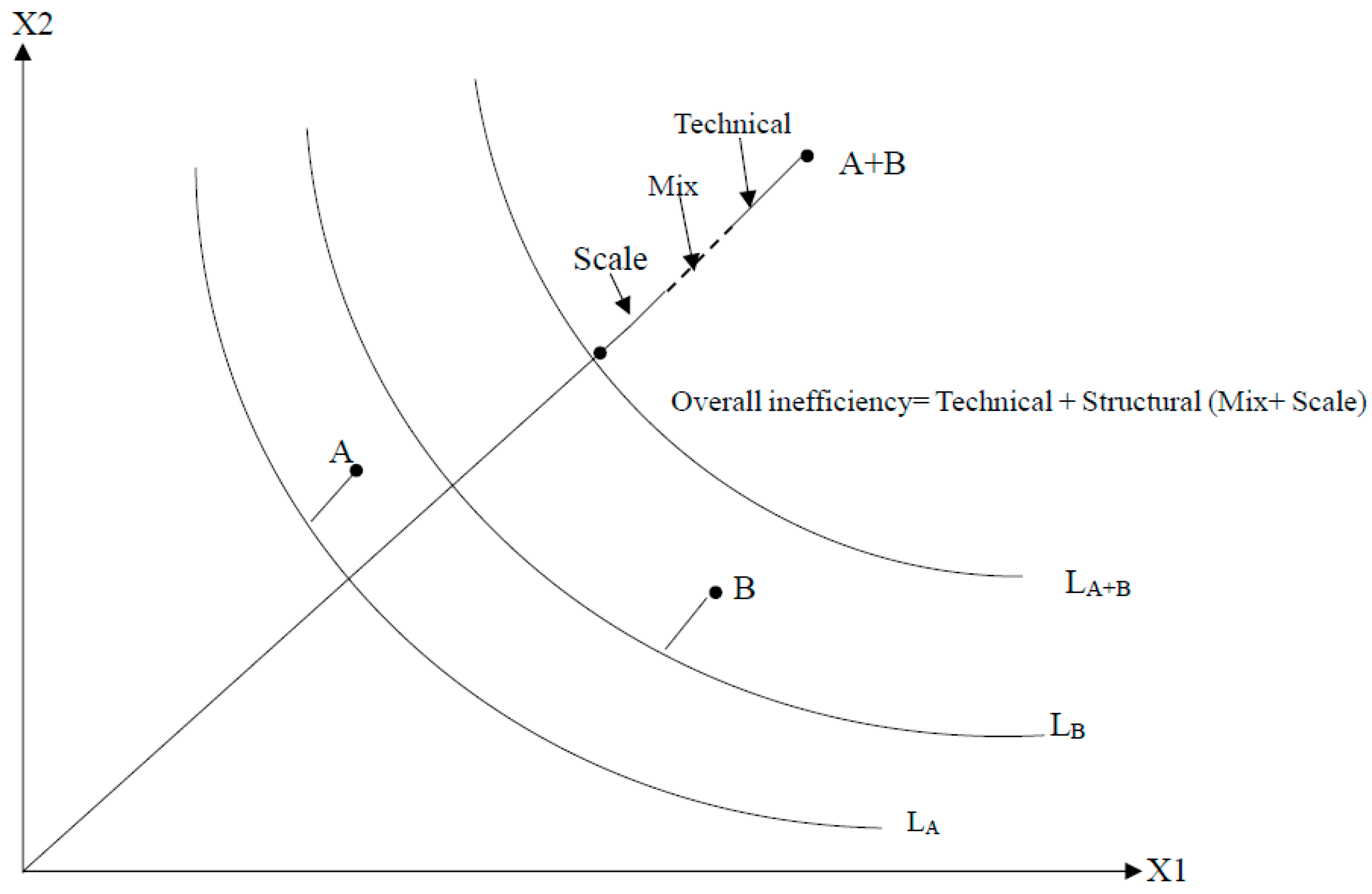
The inefficiency components for economic sub-technology are illustrated in Figure 1. Assume there are two DMUs A and B and their distances to L_A and L_B indicate technical inefficiencies, whereas the quantities of the two inputs are denoted by $x_1$ and $x_2$. When considering the operation of A and B in the case of a merger, the resulting DMU A+B can be derived from summing up the inputs and outputs of DMUs A and B. The distance between this new DMU and their aggregate production technology L_A+B is greater than (the sum of) technical inefficiencies for A and B as it contains a mix and scale effect at an aggregate level. Note that mix inefficiency occurs due to differences in the input-mix structure (if one considers the input space) and declines as these differences disappear. Thus, the merger of identical DMUs would render only a sum of their technical and scale inefficiencies. In this regard, mix inefficiency tells us about the degree of heterogeneity prevailing in the “industry” (in our case, this is the Chinese economy). However, this degree of heterogeneity is measured in terms of multiple input/output variables and considering the production frontier established by best-practice DMUs. See, for instance, Ferrier et al. [45] for more details.

3.3. Model Specification

Each term of overall inefficiency can be estimated by a corresponding linear program. At an individual level, technical inefficiency measures the distance between each province and the benchmark which can be estimated by primal LP1 under the VRS assumption. According to Murty et al. [41], we allocate equivalent weights on economic and environmental sub-technologies thus scores for each desirable and undesirable outputs (${\displaystyle \sum _{o=1}^O{\delta }_{}^o}/O$ and ${\displaystyle \sum _{p=1}^P{\theta }_{}^p}/P$) represent economic and environmental provincial technical inefficiencies:

$$\begin{array}{l}D(x_{}^m,x_{}^n,y_{}^o,z_{}^p;{\displaystyle \sum _{k=1}^K{y}_k^{}},{\displaystyle \sum _{k=1}^K{z}_k^{}})=\underset{\lambda ,\sigma ,\delta ,\theta }{Max} \frac{1}{2}({\displaystyle \sum _{o=1}^O{\delta }_{}^o}/O+{\displaystyle \sum _{p=1}^P{\theta }_{}^p}/P)\\ s.t. {\displaystyle \sum _{k=1}^K{\lambda }_k{y}_k^o\ge }{y}_{k’}^o+{\delta }_{}^o{g}_y^{}, o=1,2,\dots ,O,\\ {\displaystyle \sum _{k=1}^K{\lambda }_k}{x}_k^{c,m}\le x_{k’}^{c,m}, m=1,2,\dots ,M\\ {\displaystyle \sum _{k=1}^K{\lambda }_k}{x}_k^{d,n}\le x_{k’}^{d,n}, n=1,2,\dots ,N,\\ {\displaystyle \sum _{k=1}^K{\sigma }_k^{}{z}_k^p}\le z_{k’}^p-{\theta }_{}^p{g}_z^{}, p=1,2,\dots ,P,\\ {\displaystyle \sum _{k=1}^K{\sigma }_k^{}}{x}_k^{d,n}\ge x_{k’}^{d,n}, n=1,2,\dots ,N,\\ {\displaystyle \sum _{k=1}^K{\lambda }_k}=1,\\ {\displaystyle \sum _{k=1}^K{\sigma }_k^{}}=1,\\ {\lambda }_k\ge 0,{\sigma }_k^{}\ge 0\end{array}$$

(LP1)

Similarly, overall inefficiency can be estimated by primal LP2 under the VRS assumption at an aggregate level.

$$\begin{array}{l}D({\displaystyle \sum _{k=1}^K{x}_{}^c},{\displaystyle \sum _{k=1}^K{x}_{}^d},{\displaystyle \sum _{k=1}^{K}y},{\displaystyle \sum _{k=1}^{K}z};{\displaystyle \sum _{k=1}^K{y}_k^{}},{\displaystyle \sum _{k=1}^K{z}_k^{}})=\underset{\lambda ,\sigma ,\delta ,\theta }{Max} \frac{1}{2}({\displaystyle \sum _{o=1}^O{\delta }_{}^o}/O+{\displaystyle \sum _{p=1}^P{\theta }_{}^p}/P)\\ s.t. K{\displaystyle \sum _{k=1}^K{\lambda }_k{y}_k^o\ge }{y}_{k’}^o+{\delta }_{}^o{g}_y^{},o=1,2,..,O,\\ K{\displaystyle \sum _{k=1}^K{\lambda }_k}{x}_k^{c,m}\le x_{k’}^{c,m},m=1,2,\dots ,M,\\ K{\displaystyle \sum _{k=1}^K{\lambda }_k}{x}_k^{d,n}\le x_{k’}^{d,n},n=1,2,\dots ,N,\\ K{\displaystyle \sum _{k=1}^K{\sigma }_k^{}{z}_k^p}\le z_{k’}^p-{\theta }_{}^p{g}_z^{},p=1,2,\dots ,P,\\ K{\displaystyle \sum _{k=1}^K{\sigma }_k^{}}{x}_k^{d,n}\ge x_{k’}^{d,n},n=1,2,\dots ,N,\\ {\displaystyle \sum _{k=1}^K{\lambda }_k}=1,\\ {\displaystyle \sum _{k=1}^K{\sigma }_k^{}}=1,\\ {\lambda }_k\ge 0,{\sigma }_k^{}\ge 0\end{array}$$

(LP2)

Structural inefficiency is obtained by the distance between overall inefficiency and the summation of provincial technical inefficiencies. As discussed in the previous section, the structural inefficiency contains mix and scale elements. Mix inefficiency is calculated by considering CRS technology (i.e., both the constraints of ${\displaystyle \sum _{k=1}^K{\lambda }_k}=1$ and ${\displaystyle \sum _{k=1}^K{\sigma }_k^{}}=1$ are not considered in the estimations) and scale inefficiency is calculated residually.

3.4. Allocating Overall and Structural Inefficiencies in a Dual Model

We employ a dual program of LP2 to allocate overall inefficiency for each DMU in LP3 to measure provincial contribution to overall inefficiency. The aggregate overall inefficiency under the VRS technology is obtained as:

$$\begin{array}{l}D({\displaystyle \sum _{k=1}^K{x}_{}^c},{\displaystyle \sum _{k=1}^K{x}_{}^d},{\displaystyle \sum _{k=1}^{K}y},{\displaystyle \sum _{k=1}^{K}z};g_y^{},g_z^{}) =\\ \underset{{\pi }_x^c,{\pi }_x^d,{\pi }_y^{},{\omega }_x^d,{\omega }_z^{},v_1,v_2}{Min}({\displaystyle \sum _{m=1}^M{\pi }_x^m{x}_{k’}^{c,m}}+{\displaystyle \sum _{n=1}^N{\pi }_x^n{x}_{k’}^{d,n}}-{\displaystyle \sum _{o=1}^O{\pi }_y^o{y}_{k’}^o}-v_1)+({\displaystyle \sum _{p=1}^P{\omega }_z^p{z}_{k’}^p}-{\displaystyle \sum _{n=1}^N{\omega }_x^n{x}_{k’}^{d,n}}+v_2)\\ s.t.K{\displaystyle \sum _{o=1}^O{\pi }_y^o{y}_k^o-}K{\displaystyle \sum _{m=1}^M{\pi }_x^{c,m}{x}_k^{c,m}}-K{\displaystyle \sum _{n=1}^N{\pi }_x^{d,n}{x}_k^{d,n}}+v_1\le 0,k=1,2,\dots ,K,\\ K{\displaystyle \sum _{n=1}^N{\omega }_x^{d,n}{x}_k^{d,n}}-K{\displaystyle \sum _{p=1}^P{\omega }_z^p{z}_k^p}-v_2\le 0,k=1,2,\dots ,K,\\ {\displaystyle \sum _{o=1}^O{\pi }_y^o{g}_y^o}=0.5,\\ {\displaystyle \sum _{p=1}^P{\omega }_z^p{g}_z^p}=0.5,\\ {\pi }_y^o\ge 0,o=1,2,\dots ,O,\\ {\pi }_x^{c,m}\ge 0,m=1,2,\dots ,M,\\ {\pi }_x^{d,n}\ge 0,n=1,2,\dots ,N,\\ {\omega }_x^{d,n}\ge 0,n=1,2,\dots ,N,\\ {\omega }_z^p\ge 0,p=1,2,\dots ,P\end{array}$$

(LP3)

where ${\pi }_x^c,{\pi }_x^d,{\pi }_y^{}$ are shadow prices of non-pollution-causing and pollution-causing inputs, and desirable outputs in T₁, and ${\omega }_x^n,{\omega }_z^p$ are shadow prices of pollution-causing inputs and undesirable outputs in T₂. CRS is imposed by further restricting $v_1=0$ and $v_2=0$.

The OI can be allocated to each DMUs according to $({\displaystyle \sum _{o=1}^O{\pi }_y^o{y}_k^o-}{\displaystyle \sum _{m=1}^M{\pi }_x^m{x}_k^m}-{\displaystyle \sum _{n=1}^N{\pi }_x^n{x}_k^n}+v_1/K)$ and $({\displaystyle \sum _{n=1}^N{\omega }_x^n{x}_k^n}-{\displaystyle \sum _{p=1}^P{\omega }_z^p{z}_k^p}-v_2/K)$ at economic and environmental dimensions, respectively.

4. Results and Discussion

To evaluate economic and environmental performance in the Chinese industrial sector, we apply the methods introduced above to a balanced panel of data for China’s 30 mainland provinces, municipalities, and autonomous regions during the years of 2006–2017. Data for the Tibet Autonomous Region is not available; therefore, this paper does not include Tibet.

4.1. Data

To simplify the analysis, we divided the 30 provinces into three large economic zones based on their geographic locations: eastern region (Beijing, Tianjin, Hebei, Liaoning, Shanghai, Jiangsu, Zhejiang, Fujian, Shandong, Guangdong, Guangxi, and Hainan), inland region (Shanxi, Inner Mongolia, Jilin, Heilongjiang, Anhui, Jiangxi, Henan, Hubei, and Hunan), and western region (Sichuan, Chongqing, Guizhou, Yunnan, Shannxi, Gansu, Qinghai, Ningxia, and Xinjiang).

The methods used to evaluate the economic and environmental performance in the Chinese industrial sector are estimated using three inputs (labor force, capital stock, energy consumption) one desirable output (value-added) and one undesirable output (carbon dioxide emission).

Labor force is defined as the number of labor factors invested in industrial production. The data come from the statistical yearbooks and labor statistics yearbooks [49,50] of various provinces in China.

Capital stock is defined as the amount of capital employed in industrial production, which is calculated according to the perpetual inventory method [51]. The 2006–2017 fixed asset investment data comes from the China Fixed Assets Investment Statistical Yearbook [52]. The depreciation rate varies significantly among Chinese provinces, and its influence on capital stock estimation cannot be ignored. This paper calculates the depreciation rate of each province according to the fixed asset investment structure data of each provincial district [53]. The details for depreciation rate are available in

Table A1. Depreciation rate for the provinces.

Province	Depreciation Rate (%)
Beijing	9.83
Tianjin	10.47
Hebei	11.02
Shanxi	10.7
Inner Mongolia	10.28
Liaoning	10.62
Jilin	10.81
Heilongjiang	10.66
Shanghai	10.47
Jiangsu	11.19
Zhejiang	10.7
Anhui	10.34
Fujian	10.54
Jiangxi	10.48
Shandong	11.02
Henan	10.25
Hubei	10.56
Hunan	10.12
Guangdong	10.4
Guangxi	10.32
Hainan	10.49
Chongqing	9.81
Sichuan	10.25
Guizhou	10.39
Yunnan	9.78
Tibet	8.86
Shaanxi	9.93
Gansu	10.21
Qinghai	9.67
Ningxia	10.59
Xinjiang	10.22

in Appendix A.

Energy consumption is defined as the energy consumption of industrial terminals. We selected the terminal consumption of all 19 types of energy in each sector provided by the China Energy Statistics Yearbook [54] and converted it to 10,000 tons of standard coal according to the standard coal conversion coefficient.

Value-added is defined as the value of the total output of all production activities of industrial enterprises after deducting the value of the physical products and services consumed or transferred in the production process during the reporting period. This paper uses the constant price of 1999 as the benchmark price to measure the desirable output of the industry. The data come from the China Industrial Economics Statistical Yearbook and the China Statistical Yearbook [50,55].

The International Panel on Climate Change [56] described the calculation of the energy-related CO₂ emissions based on the amount of fuel combusted and the emission factor. This paper uses the IPCC [56] method to estimate carbon dioxide emissions data for 2006–2017 in 30 provinces in mainland China. The data come from the China Energy Statistical Yearbook 2000–2018 [54]. The yearbook provides data of both fossil and non-fossil energy consumptions. However, the types of energy consumptions are different due to data availability. In detail, coal, coke, coke oven gas, other gas, crude oil, gasoline, and kerosene are considered into the computation of CO₂ emissions during 2006–2009. While in 2010–2017, additional energy sources, such as blast furnace gas, converter gas, and liquefied natural gas, were also included. To avoid the double counting issue, some intermediate energy consumptions are excluded from computation, such as electricity used.

Table 1. Annual growth rates of inputs and outputs (%, 2006–2017).

Type	Variable	Eastern	Inland	Western	China
Inputs	Labor	1.96	2.62	2.66	2.25
	Capital stock	16.00	20.94	19.33	17.97
	Energy consumption	3.23	2.53	5.60	3.47
Desirable output	Value added	9.46	12.00	13.75	10.72
Undesirable output	CO2	3.99	4.44	5.88	4.47

Note: All monetary variables have been to deflated to the constant price level.

briefly describes the annual growth rates of the output and input variables for the three large economic groups and the whole of China. The value-added trends surpass 10.7% while the growth rates for CO₂ emissions are nearly 4.5%. Consequently, slight decreases in CO₂ emissions per unit of the value-added unit can be observed for all areas. Whether it is value added or CO₂, the growth rate in the western region is much higher than that in the inland and eastern regions. This shows that although the overall level of economic development is low, the area of the west is a vital force in China’s industrial production.

Compared to the value-added trends, the labor force is characterized by slow growth rates of nearly 2%. As a result, labor productivity improved significantly for the sample period. At the same time, the capital stock grows at a rate of around 16% or more, which may be due to China’s financial opportunities and preferential policies that are conducive to industrial development and attracting domestic and foreign investors. In terms of energy consumption, national energy consumption is around 3.5%. However, capital stock is more than 19% in the western region, energy consumption and CO₂ emissions in the west part are the highest in all areas, indicating that the west region features an extensive growth pattern characterized by high investment, high energy consumption, and high emissions.

4.2. Empirical Results and Discussion

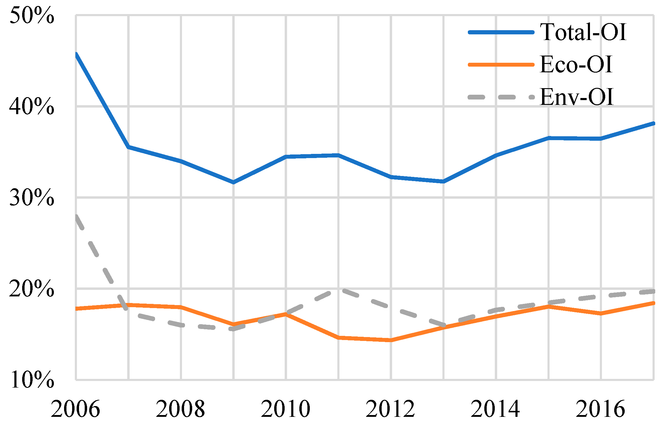
Dynamics in the country-wide total OI (i.e., the sum of the economic and environmental inefficiencies each comprising technical, mix and scale terms) is given in Figure 2. As one can note, the trend in the total OI follows a U-shape for the Chinese industry sector. First, there was a decline in inefficiency during 2006–2009 (the total OI went down from some 46 to 32%). Second, there was a “steady” sub-period of 2009–2013 when the total OI fluctuated around 32%. Third, the sub-period of 2013–2017 marked an upward trend of the total OI. During the latter phase, the total OI went up from 32 to 38%.

The by-production technology allows for accounting for the two types of the OI, namely the economy- and environment-related OI. The trends depicted in Figure 2 imply these two types of inefficiency were quite close in their trajectories (both in terms of averages and variation). However, there had been certain discrepancies during different phases. In the first sub-period, the environmental performance was the major contributor of changes in the total OI, whereas the economic OI remained rather stable. Throughout the second sub-period, economic and environmental OI moved to the opposite directions. Finally, the directions of changes in the economic and environment OI coincided during the third sub-period.

A more detailed decomposition of the OI is presented in

Table 2. Industry inefficiency scores among regions (%, mean values during 2006–2017).

Region	Time Period	OI		TI		MIX		SCALE
		Eco	Env	Eco	Env	Eco	Env	Eco	Env
Eastern	2006	7.51	15.09	2.72	7.90	5.45		−0.66	7.19
	2017	5.98	8.79	3.47	5.87	5.22		−2.71	2.92
	Mean	5.93	8.73	2.45	5.35	5.03		−1.55	3.38
Inland	2006	5.98	8.71	3.73	6.61	1.61		0.64	2.10
	2017	6.99	7.59	5.02	7.18	3.19		−1.22	0.41
	Mean	6.08	6.80	4.34	6.30	3.21		−1.48	0.50
Western	2006	4.32	4.12	2.86	3.72	0.81		0.64	0.40
	2017	5.45	3.33	2.96	3.33	0.89		1.60	0.00
	Mean	4.89	3.06	2.66	3.03	1.16		1.06	0.03
China	2006	17.81	27.92	9.31	18.24	7.88		0.63	9.68
	2017	18.42	19.70	11.46	16.38	9.29		−2.33	3.32
	Mean	16.89	18.59	9.46	14.68	9.40		−1.97	3.91

Note: as there is only one pollution-generating input and one bad output in the environmental sub-technology, there is no mix inefficiency associated with the latter sub-technology.

. On average, the contribution of the economic OI is lower than that of the environmental OI (16.9 and 18.6% respectively). The same pattern persists for all types of inefficiency. Region-wise, the western region shows the lowest total OI (some 8% accounting for both economic and environmental OI), whereas the contribution of the inland region is 12.9% and that of the eastern region is 14.7%, which was also found by Wang et al. [14,16], Yang et al. [20], Wu et al. [28] and Lin and Zheng [37]. Thus, the performance gaps should be addressed by considering different regions in China. Turning to the sources of the OI, the environmental inefficiency prevails over the economic inefficiency in the eastern and inland regions. On the contrary, the western region shows an opposite pattern with economic and environmental OI standing at 4.9 and 3.1% respectively. Ding et al. [31] obtained a similar result when examining industrial water and energy utilization efficiency. Thus, a higher level of economic development induced both lower total OI and minimal contribution of environmental OI.

Note that the eastern region shows a relatively low average economic OI if compared to the other regions, yet its total OI is the highest among the regions. Thus, environmental performance and the misallocation of resources constitute the underlying causes of total inefficiency. Therefore, structural reforms are necessary in addition to improvements in production processes in the eastern region.

Yet another nuance is the estimates of the scale inefficiency. As one can note, environmental scale inefficiency is positive in all the instances, whereas economic scale inefficiency is negative for all regions but the western region. According to Li et al. [57], the extensive expansion of heavy industry in China was the reason of the decline in productivity, which also caused negative growth in economic scale efficiency. Thus, the eastern and inland regions are closer to optimal scale size even though their mix efficiency is lower. In addition, scale efficiency related to environmental sub-technology is much higher for the aforementioned two regions if opposed to the western region. Thus, accounting for the two sub-technologies unveils differences in the sources of the scale inefficiency across different regions.

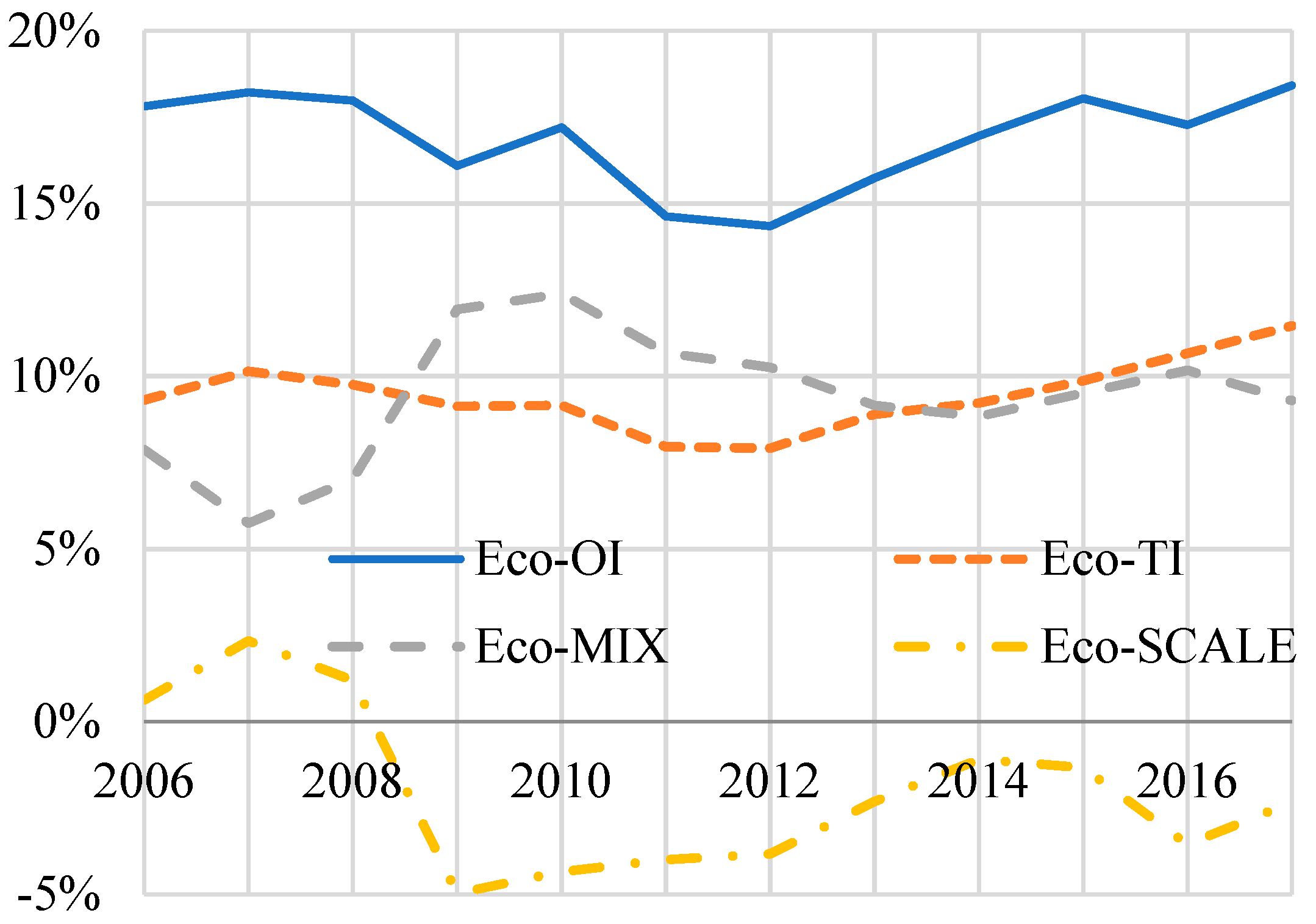
We further look at the trends in the inefficiency across different sources and regions. Figure 3 presents the country-wide dynamics in the economic OI and its decomposition into technical, scale and mix inefficiencies. Scale and mix inefficiencies followed asymmetric trajectories during 2006–2017 without clear direction. Technical inefficiency generally increased over the same period. Therefore, for the economic sub-technology, improvements in productivity remain the major objective. Overall economic inefficiency has kept steadily increasing since 2012.

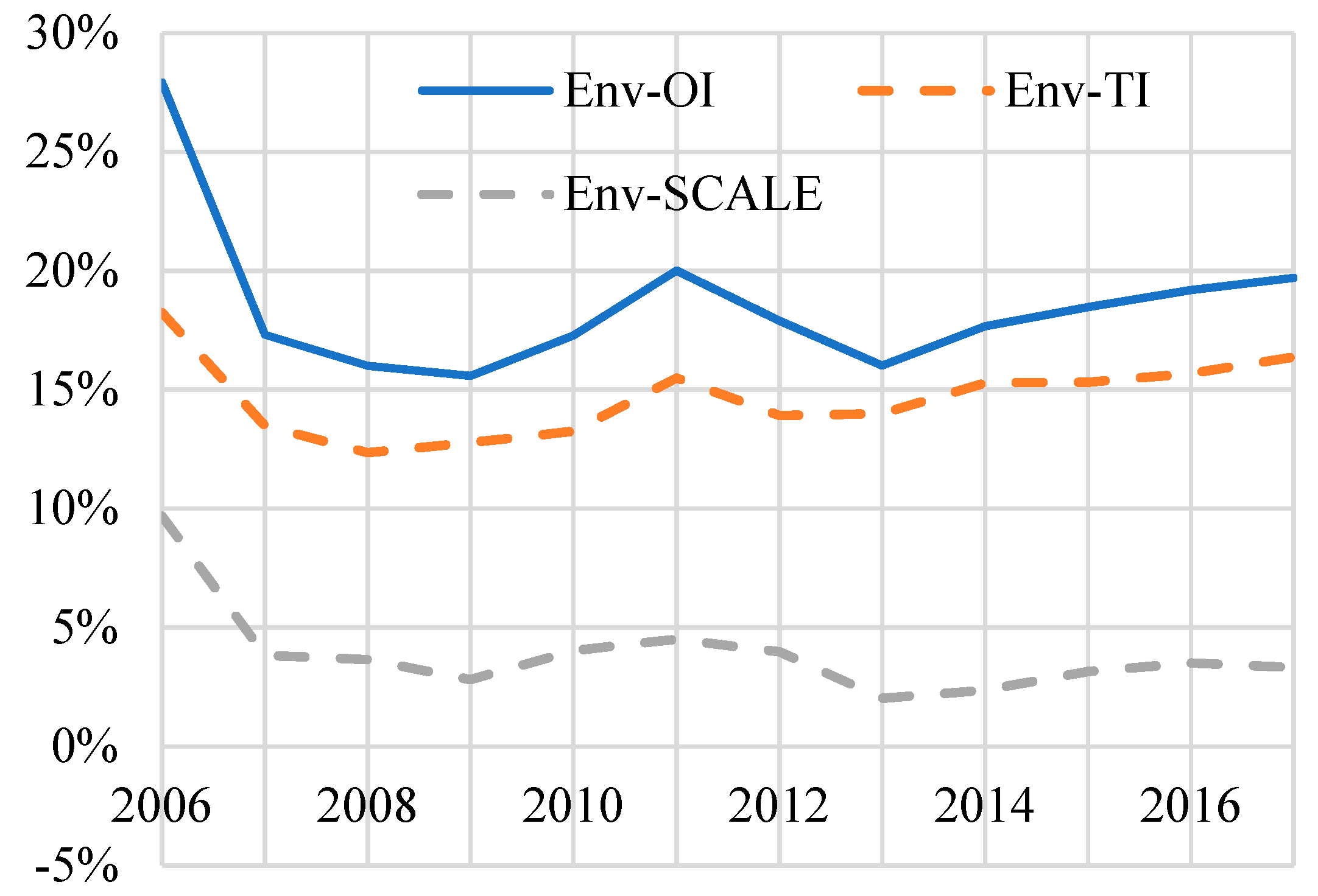
The trends in environmental inefficiency are outlined in Figure 4. Environmental inefficiency declined during 2006–2007 and remained rather stable afterwards. Technical inefficiency remained the major contributor towards overall environmental inefficiency throughout 2006–2017. The trends in technical and scale environmental inefficiency generally coincided during the period covered.

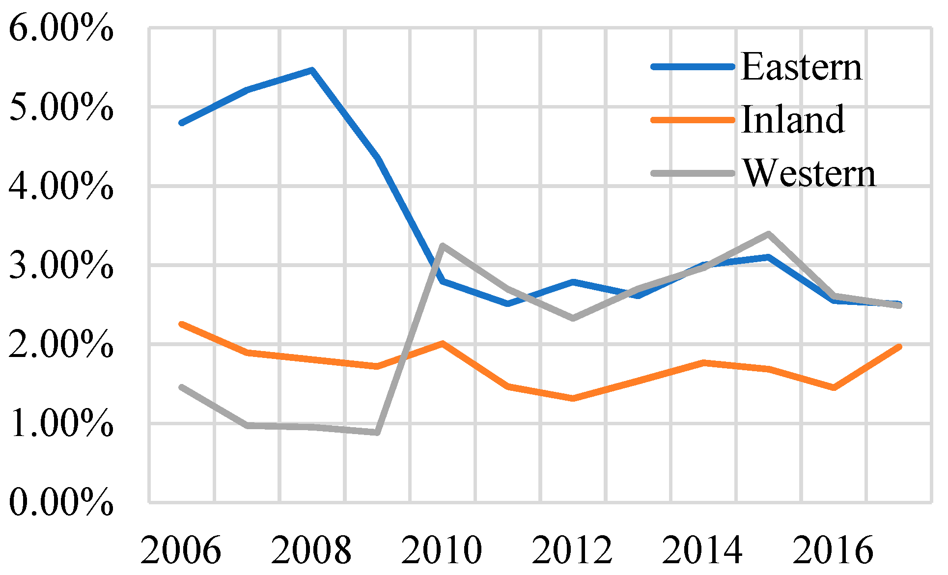
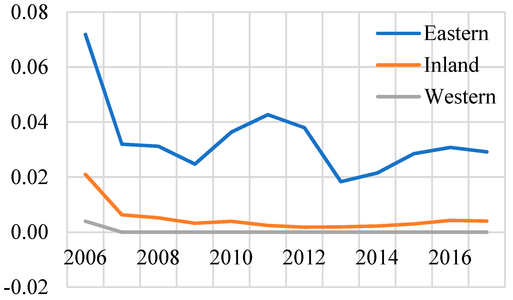
The regional approach can be taken to ascertain the structural inefficiency in China’s economy. Indeed, such an approach is highly relevant as structural efficiency deals with the issues of resource misallocation among the decision making units (which are provinces in our case). Thus, Figure 5 and Figure 6 embark on the region-wise analysis of structural inefficiency in China’s industry. Recall that structural inefficiency comprises of mix and scale inefficiency in our setting.

The comparison of the dynamics in structural inefficiency related to economic sub-technology across the regions is presented in Figure 5. Obviously, the western region became less structurally efficient following the economic crisis of 2008. The eastern region, on the contrary, managed to decrease structural inefficiency during 2006–2010, and similar results are also found in the whole Chinese economy by Boussemart et al. [46] and in the agricultural sector by Shen et al. [35]. Throughout 2010–2017, both eastern and western regions maintained rather similar levels (and directions) of structural inefficiency. The lowest economic structural inefficiency was maintained in the inland region during 2006–2017. Thus, the eastern and western regions require reallocation of production capacities in order to reduce the associated structural inefficiency.

The region-wise decomposition of environmental structural inefficiency is given in Figure 6. The eastern region followed a downward trend in the environmental structural efficiency during 2006–2017, yet remained a region with the highest value among the three regions for the whole period covered. As regards to the inland and western regions, their contribution towards environmental structural inefficiency remained close to zero for 2008–2017. Accordingly, the scale of the operation of the pollution-generating industries needs to be further optimized in the eastern region (as the latter type of inefficiency is solely captured by structural inefficiency for the environmental sub-technology in our setting).

Table 3. Average growth rates in inefficiency scores, 2006–2017.

Region	China		Eastern		Inland		Western
	Coefficient	t-Value	Coefficient	t-Value	Coefficient	t-Value	Coefficient	t-Value
OIEco	−0.01	−0.049	−0.20	−2.338	0.05	0.972	0.15	2.980
OIEnv	−0.18	−0.643	−0.20	−1.191	0.03	0.322	0.00	−0.044
TIEco	0.10	1.205	0.05	1.314	0.08	2.299	−0.03	−1.225
TIEnv	0.12	0.807	0.00	−0.048	0.11	1.947	0.01	0.497
MIXEco	0.16	1.036	0.09	1.018	0.07	0.795	0.00	−0.057
SCALEEco	−0.27	−1.438	−0.35	−3.080	−0.11	−1.085	0.18	2.793
SCALEEnv	−0.30	−2.072	−0.20	−1.948	−0.08	−2.132	−0.02	−1.732

Note: growth rates are based on the log-linear trends; coefficients significant at the level of 5% are boldfaced.

aggregates the results regarding the trends in different components of economic and environmental efficiency across the three regions. The growth rates are based on the stochastic trends which also allow for statistical inference. Clearly, the eastern region followed a significantly downward trend in the overall economic inefficiency (−0.2 p.p. annually) with the scale component being the sole term following a significant trend (−0.35 p.p. annually). The western region followed a significantly upward trend in overall economic inefficiency (0.15 p.p. annually) which implies the need for productivity gains in the industry sector there. In this case, the scale component was also significant (the annual increase of some 0.18 p.p.).

The inland region experienced technical efficiency losses as represented by significantly positive rates of growth in the inefficiencies associated with both economic and environmental sub-technologies (0.08 p.p. and 0.11 p.p. respectively). The scale component associated with the environmental sub-technology was significantly changing for the whole of China and the three regions. In all instances, significantly negative coefficients indicated improvements in environmental efficiency due to the re-allocation of pollution-generating activities. In general, one can note a substantial degree of disparity in terms of inefficiency levels among Chinese regions. Specifically, eastern regions exhibit a steeper decline in inefficiencies if compared to inland and western areas (where an increase can be observed). This pattern is consistent with studies by Sun et al. [58], Wu et al. [12], and Zhou et al. [59].

5. Conclusions and Implications

In this paper, we evaluated performance in the Chinese industry sector across 30 provinces from 2006 to 2017. Based on the by-production model, performance in the Chinese industry sector was measured by taking economic and environmental dimensions into consideration simultaneously. At the aggregate level, overall inefficiency scores in the Chinese industry sector was decomposed into three elements: technical, scale and mix inefficiency. The empirical results indicate that economic and environmental performance plays almost the same role for Chinese industry inefficiency during the period covered. Compared with economic sub-technology, overall inefficiency is higher for environmental sub-technology. Correspondingly, the technical and scale inefficiencies for environmental sub-technology are also higher if compared to those for the economic sub-technology. The results illustrate that environmental performance in the Chinese industry sector still requires further improvement. While promoting the development of the industrial sector, the Chinese government needs to pay more attention to improving environmental efficiency there. This firstly relies on the creation of more environment-friendly energy systems. In this regard, the creation of smart grids would allow a transition towards cleaner energy and, thus, lower environmental inefficiency. Modern technologies, e.g., blockchain, may allow for the creation of micro-grids allowing Chinese industry to reduce the environmental pressures. The government could support investment into equipment related to the construction of smart grids in the inland and eastern regions as these regions showed the highest mean overall environmental inefficiency for 2006–2017.

Innovative decomposition allowed for the isolation of structural inefficiency (i.e., mix and scale inefficiency). The results suggest that economic structural inefficiency remains important in the developed western region. The eastern region requires a reduction in structural inefficiency related to both economic and environmental sub-technologies. The central government could initiate support and regulatory measures inducing spatial shifts of production capacities to approach a more productive structure. Measures such as emissions trading are important for the eastern region in order to reduce structural environmental inefficiency. As regards to scale and environmental economic inefficiency prevailing in both western and eastern regions, support measures should be developed to introduce modern production facilities, whereas backward facilities should be discouraged by applying restrictive fiscal measures.

References

- National Bureau of Statistics in China. 2019. Available online: http://www.stats.gov.cn/ (accessed on 12 August 2018).
- Chen, J.D.; Cheng, S.L.; Nikic, V.; Song, M.L. Quo Vadis? Major Players in Global Coal Consumption and Emissions Reduction. Transform. Bus. Econ. 2018, 17, 112–132. [Google Scholar]
- Piłatowska, M.; Włodarczyk, A. Decoupling Economic Growth from Carbon Dioxide Emissions in the EU Countries. Montenegrin J. Econ. 2018, 14, 7–26. [Google Scholar] [CrossRef]
- Yin, C.B. Environmental efficiency and its determinants in the development of China’s western regions in 2000–2014. Chin. J. Popul. Resour. Environ. 2017, 15, 157–166. [Google Scholar] [CrossRef]
- Liu, C.-C.; Cheng, A.-C.; Chen, S.-H. A study for sustainable development in optoelectronics industry using multiple criteria decision making methods. Technol. Econ. Dev. Econ. 2017, 23, 221–242. [Google Scholar] [CrossRef]
- Sueyoshi, T.; Yuan, Y.; Li, A.; Wang, D. Social sustainability of provinces in China: A data envelopment analysis (DEA) window analysis under the concepts of natural and managerial disposability. Sustainability 2017, 9, 2078. [Google Scholar] [CrossRef]
- Song, M.; Peng, J.; Wang, J.; Dong, L. Better resource management: An improved resource and environmental efficiency evaluation approach that considers undesirable outputs. Resour. Conserv. Recycl. 2018, 128, 197–205. [Google Scholar] [CrossRef]
- Song, M.; Fisher, R.; Kwoh, Y. Technological challenges of green innovation and sustainable resource management with large scale data. Technol. Forecast. Soc. Chang. 2019, 144, 361–368. [Google Scholar] [CrossRef]
- Fang, S.; Ji, X.; Ji, X.; Wu, J. Sustainable urbanization performance evaluation and benchmarking: An efficiency perspective. Manag. Environ. Qual. 2018, 29, 240–254. [Google Scholar] [CrossRef]
- Chen, L.; Wu, F.M.; Wang, Y.M.; Li, M.J. Analysis of the environmental efficiency in China based on the DEA cross-efficiency approach under different policy objectives. Expert Syst. 2019, e12461. [Google Scholar] [CrossRef]
- Wu, J.; Li, M.J.; Zhu, Q.Y.; Zhou, Z.X.; Liang, L. Energy and environmental efficiency measurement of China’s industrial sectors: A DEA model with non-homogeneous inputs and outputs. Energy Econ. 2019, 78, 468–480. [Google Scholar] [CrossRef]
- Wu, Y.; Su, J.R.; Li, K.; Sun, C.W. Comparative study on power efficiency of China’s provincial steel industry and its influencing factors. Energy 2019, 175, 1009–1020. [Google Scholar] [CrossRef]
- Shao, L.G.; Yu, X.; Feng, C. Evaluating the eco-efficiency of China’s industrial sectors: A two-stage network data envelopment analysis. J. Environ. Manag. 2019, 247, 551–560. [Google Scholar] [CrossRef] [PubMed]
- Wang, K.; Yu, S.; Zhang, W. China’s regional energy and environmental efficiency: A DEA window analysis based dynamic evaluation. Math. Comput. Model. 2013, 58, 1117–1127. [Google Scholar] [CrossRef]
- Wang, K.; Wei, Y.M.; Zhang, X. Energy and emissions efficiency patterns of Chinese regions: A multi-directional efficiency analysis. Appl. Energy 2013, 104, 105–116. [Google Scholar] [CrossRef]
- Wang, K.; Lu, B.; Wei, Y.M. China’s regional energy and environmental efficiency: A range-adjusted measure based analysis. Appl. Energy 2013, 112, 1403–1415. [Google Scholar] [CrossRef]
- Wang, X.M.; Ding, H.; Liu, L. Eco-efficiency measurement of industrial sectors in China: A hybrid super-efficiency DEA analysis. J. Clean. Prod. 2019, 229, 53–64. [Google Scholar] [CrossRef]
- Shen, N.; Liao, H.L.; Deng, R.M.; Wang, Q.W. Different types of environmental regulations and the heterogeneous influence on the environmental total factor productivity: Empirical analysis of China’s industry. J. Clean. Prod. 2019, 211, 171–184. [Google Scholar] [CrossRef]
- Feng, C.; Wang, M.; Zhang, Y.; Liu, G.C. Decomposition of energy efficiency and energy-saving potential in China: A three-hierarchy meta-frontier approach. J. Clean. Prod. 2018, 176, 1054–1064. [Google Scholar] [CrossRef]
- Yang, L.; Ouyang, H.; Fang, K.; Ye, L.; Zhang, J. Evaluation of regional environmental efficiencies in China based on super-efficiency-DEA. Ecol. Indic. 2015, 51, 13–19. [Google Scholar] [CrossRef]
- Du, J.; Chen, Y.; Huang, Y. A modified Malmquist-Luenberger productivity index: Assessing environmental productivity performance in China. Eur. J. Oper. Res. 2018, 269, 171–187. [Google Scholar] [CrossRef]
- Zhang, A.; Li, A.; Gao, Y. Social sustainability assessment across provinces in China: An analysis of combining intermediate approach with data envelopment analysis (DEA) window analysis. Sustainability 2018, 10, 732. [Google Scholar] [CrossRef]
- Sueyoshi, T.; Yuan, Y.; Goto, M. A literature study for DEA applied to energy and environment. Energy Econ. 2017, 62, 104–124. [Google Scholar] [CrossRef]
- Meng, F.Y.; Fan, L.W.; Zhou, P.; Zhou, D.Q. Measuring environmental performance in China’s industrial sectors with non-radial DEA. Math. Comput. Model. 2013, 58, 1047–1056. [Google Scholar] [CrossRef]
- Wang, J.; Zhao, T.; Zhang, X.H. Environmental assessment and investment strategies of provincial industrial sector in China—Analysis based on DEA model. Environ. Impact Assess. Rev. 2016, 60, 156–168. [Google Scholar] [CrossRef]
- Zhang, T. Frame work of data envelopment analysis—A model to evaluate the environmental efficiency of China’s industrial sectors. Biomed. Environ. Sci. 2009, 22, 8–13. [Google Scholar] [CrossRef]
- Zhang, N.; Wang, B.; Liu, Z. Carbon emissions dynamics, efficiency gains, and technological innovation in China’s industrial sectors. Energy 2016, 99, 10–19. [Google Scholar] [CrossRef]
- Wu, J.; Zhu, Q.Y.; Liang, L. CO2 emissions and energy intensity reduction allocation over provincial industrial sectors in China. Appl. Energy 2016, 166, 282–291. [Google Scholar] [CrossRef]
- Xie, B.C.; Duan, N.; Wang, Y.S. Environmental efficiency and abatement cost of China’s industrial sectors based on a three-stage data envelopment analysis. J. Clean. Prod. 2017, 153, 626–636. [Google Scholar] [CrossRef]
- Wu, F.; Fan, L.W.; Zhou, P.; Zhou, D.Q. Industrial energy efficiency with CO2 emissions in China: A nonparametric analysis. Energy Policy 2012, 49, 164–172. [Google Scholar] [CrossRef]
- Ding, T.; Wu, H.; Dai, Q.; Zhou, Z.; Tan, C. Environmental efficiency analysis of urban agglomerations in China: A non-parametric meta-frontier approach. Emerg. Mark. Financ. Trade 2019. [Google Scholar] [CrossRef]
- Lam, P.L.; Shiu, A. A data envelopment analysis of the efficiency of China’s thermal power generation. Util. Policy 2001, 10, 75–83. [Google Scholar] [CrossRef]
- Yang, H.; Pollitt, M. Incorporating both undesirable outputs and uncontrollable variables into DEA: The performance of Chinese coal-fired power plants. Eur. J. Oper. Res. 2009, 197, 1095–1105. [Google Scholar] [CrossRef] [Green Version]
- Zhang, T. Environmental performance in China’s agricultural sector: A case study in corn production. Appl. Econ. Lett. 2008, 15, 641–645. [Google Scholar] [CrossRef]
- Shen, Z.Y.; Baležentis, T.; Chen, X.L.; Valdmanis, V. Green growth and structural change in Chinese agricultural sector during 1997–2014. China Econ. Rev. 2018, 51, 83–96. [Google Scholar] [CrossRef]
- Feng, C.; Wang, M. Analysis of energy efficiency in China’s transportation sector. Renew. Sustain. Energy Rev. 2018, 94, 565–575. [Google Scholar] [CrossRef]
- Lin, B.Q.; Zheng, Q.Y. Energy efficiency evolution of China’s paper industry. J. Clean. Prod. 2017, 140, 1105–1117. [Google Scholar] [CrossRef]
- Li, J.; See, K.F.; Chi, J. Water resources and water pollution emissions in China’s industrial sector: A green-biased technological progress analysis. J. Clean. Prod. 2019, 229, 1412–1426. [Google Scholar] [CrossRef]
- Yu, A.; Jia, G.; You, J.; Zhang, P. Estimation of PM2.5 concentration efficiency and potential public mortality reduction in urban China. Int. J. Environ. Res. Public Health 2018, 15, 529. [Google Scholar] [CrossRef] [Green Version]
- Färe, R.; Grosskopf, S.; Pasurka, C.A., Jr. Environmental production functions and environmental directional distance functions. Energy 2007, 32, 1055–1066. [Google Scholar] [CrossRef]
- Murty, S.; Russell, R.R.; Levkoff, S.B. On modeling pollution-generating technologies. J. Environ. Econ. Manag. 2012, 64, 117–135. [Google Scholar] [CrossRef] [Green Version]
- Murty, S.; Russell, R.R. On Modeling Pollution Generating Technologies; Discussion Papers Series; Department of Economics, University of California: Riverside, CA, USA, 2002; pp. 1–18. [Google Scholar]
- Hackman, S.T. Production Economics: Integrating the Microeconomic and Engineering Perspectives; Springer: Berlin/Heidelberg, Germany, 2008. [Google Scholar]
- Chambers, R.; Chung, Y.; Färe, R. Benefit and distance functions. J. Econ. Theory 1996, 70, 407–419. [Google Scholar] [CrossRef]
- Ferrier, G.; Leleu, H.; Valdmanis, V. The impact of CON regulation on hospital efficiency. Health Care Manag. Sci. 2010, 83, 84–100. [Google Scholar] [CrossRef] [PubMed]
- Boussemart, J.P.; Leleu, H.; Shen, Z.Y. Environmental growth convergence among Chinese regions. China Econ. Rev. 2015, 34, 1–18. [Google Scholar] [CrossRef]
- Shen, Z.Y.; Boussemart, J.P.; Leleu, H. Aggregate green productivity growth in OECD’s countries. Int. J. Prod. Econ. 2017, 189, 30–39. [Google Scholar] [CrossRef] [Green Version]
- Li, S.K. Relations between convexity and homogeneity in multi-output technologies. J. Math. Econ. 1995, 24, 311–318. [Google Scholar] [CrossRef]
- National Bureau of Statistics of China. China Labor Statistical Yearbook; China Statistics Press: Beijing, China, 1996–2018.
- National Bureau of Statistics of China. China Statistical Yearbook; China Statistics Press: Beijing, China, 1996–2018. [Google Scholar]
- Shan, H. Reestimating the capital stock of China: 1952-2006. J. Quant. Tech. Econ. 2008, 10, 12–20. (In Chinese) [Google Scholar]
- National Bureau of Statistics of China. Yearbook of the Chinese Investment in Fixed Assets; China Statistics Press: Beijing, China, 1996–2018.
- Zong, Z.L.; Liao, Z.D. Re-estimation of capital stock of three inter provincial industries in China: 1978–2011. J. Guizhou Univ. Financ. Econ. 2014, 3, 8–16. (In Chinese) [Google Scholar]
- National Bureau of Statistics of China. China Energy Statistical Yearbook; China Statistics Press: Beijing, China, 1996–2018.
- National Bureau of Statistics of China. China Industry Statistical Yearbook; China Statistics Press: Beijing, China, 1996–2018.
- IPCC. IPCC Guidelines for National Greenhouse Gas Inventories; Eggleston, H.S., Buendia, L., Miwa, K., Ngara, T., Tanabe, K., Eds.; Prepared by the National Greenhouse Gas Inventories Programme; IGES: Hayama, Japan, 2006. [Google Scholar]
- Li, W.W.; Wang, W.P.; Wang, Y.; Ali, M. Historical growth in total factor carbon productivity of the Chinese industry—A comprehensive analysis. J. Clean. Prod. 2018, 170, 471–485. [Google Scholar] [CrossRef]
- Sun, J.C.; Du, T.; Sun, W.Q.; Na, H.M.; He, J.F.; Qiu, Z.Y.; Yuan, Y.X.; Li, Y.N. An evaluation of greenhouse gas emission efficiency in China’s industry based on SFA. Sci. Total Environ. 2019, 690, 1190–1202. [Google Scholar] [CrossRef]
- Zhou, Z.X.; Xu, G.C.; Wang, C.; Wu, J. Modeling undesirable output with a DEA approach based on an exponential transformation: An application to measure the energy efficiency of Chinese industry. J. Clean. Prod. 2019, 236, 117717. [Google Scholar] [CrossRef]
Figure 1.
An illustration of the decomposition of overall inefficiency.
Figure 2.
Overall inefficiencies in the Chinese industry sector, 2006–2017.
Figure 3.
Decomposition of economic performance, 2006–2017.
Figure 4.
Decomposition of environmental performance, 2006–2017.
Figure 5.
Economic structural inefficiency among regions, 2006–2017.
Figure 6.
Environmental structural inefficiency among regions, 2006–2017.