Failure Analysis of the Water Supply Network in the Aspect of Climate Changes on the Example of the Central and Eastern Europe Region


Abstract
:1. Introduction
2. Materials and Methods
- Ti—this index refers to the temperature range <ti;ti+1, and its value is the average temperature for a given range,
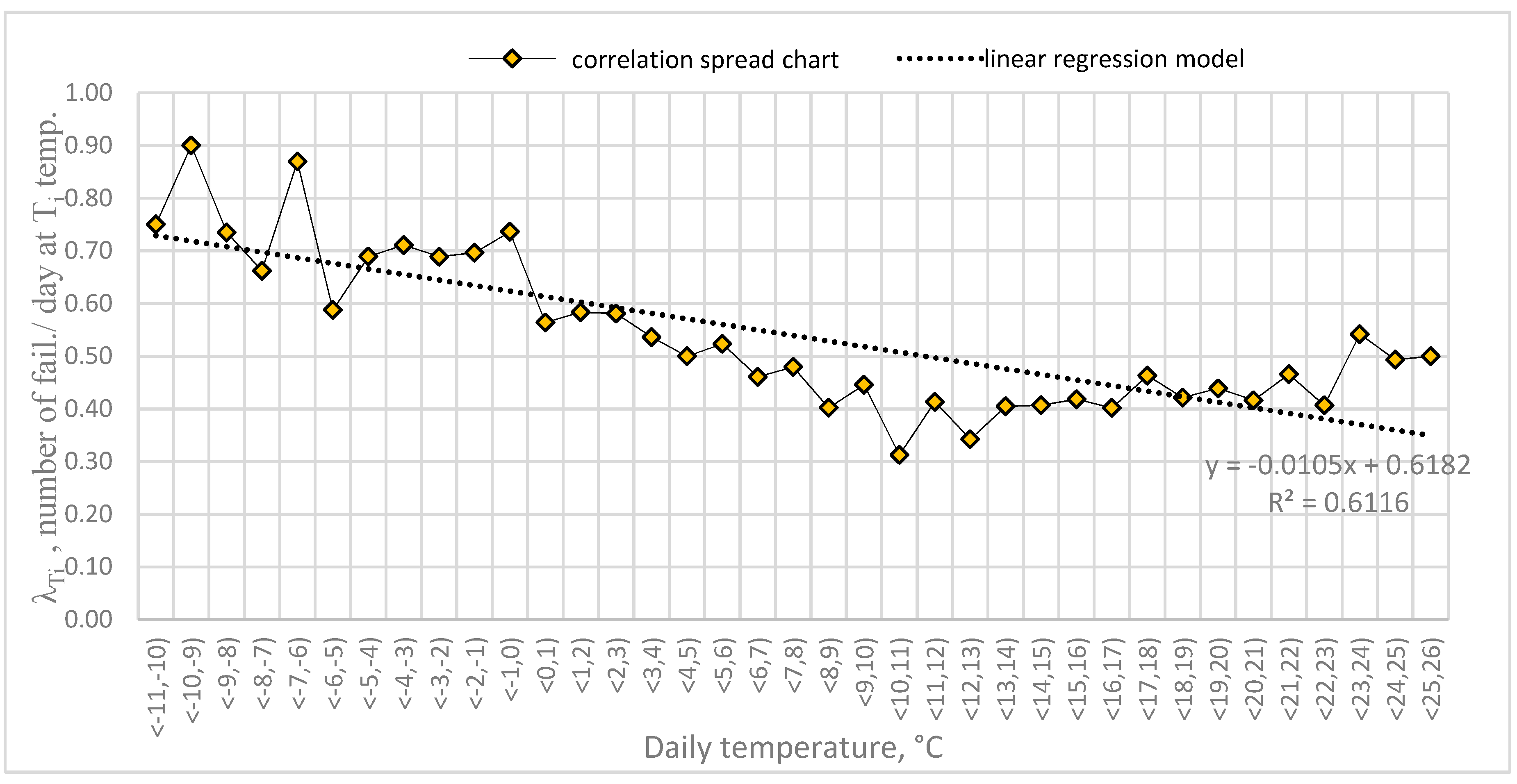
- λTi—the failure rate at a given air temperature Ti,
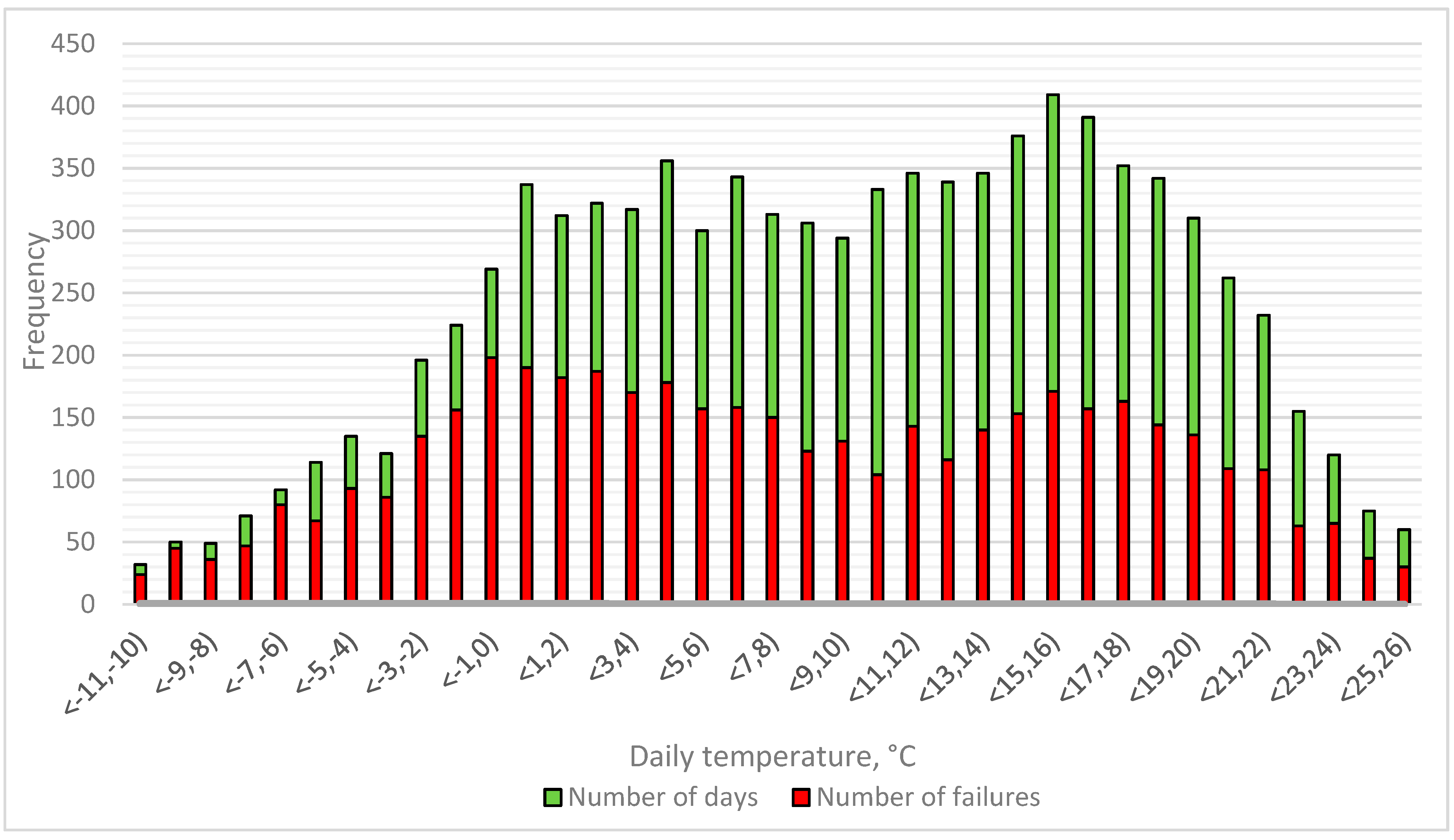
- nTi—number of failures occurring at daily air temperature Ti, and
- dTi—number of days with daily air temperature Ti.
- dav—the average number of days per unit temperature (169), and
- dσ—the standard deviation of the number of days per unit temperature (146).
- r—the linear correlation coefficient, and
- n—sample size.
- λ%—the percentage share of the failure rate dependent on the temperature change in the total failure rate,
- ax + b—the linear regression equation, and
- λb—the absolute failure rate.
- λTiH—the failure rate at a given air temperature Ti, associated with the temperature changes,
- λ%—the percentage share of the failure rate related to the temperature changes, and
- λTi—the failure rate at a given air temperature Ti.
- RCP 2.6—inhibiting greenhouse gas emission to the level of 2.6 W/m2,
- RCP 4.5 and RCP 6.0—stabilization of greenhouse gas emission at 4.5 W/m2 or 6.0 W/m2, and
- RCP 8.5—high increase in greenhouse gas emission to 8.5 W/m2.
- tp—predicted temperature,
- th—historical temperature, and
- Δts—predicted temperature increase.
- nfTi—number of failures in the forecasted period f (2036–2050 or 2086–2100) for a given air temperature Ti,
- dfTi—number of days in the forecasted period f (2036–2050 or 2086–2100) with daily air temperature Ti, and
- λTiH—the failure rate at a given air temperature Ti, associated with the temperature changes.
- —e total number of failures resulting from the temperature changes in the period 2004–2018,
- —e total number of failures resulting from the temperature changes over the forecasted period 2036–2050 or 2086–2100,
- 4432—the total number of failures in the period 2004–2018, for the temperature range covered by the analysis <−11, 26) °C.
3. Results
4. Discussion
5. Conclusions
Author Contributions
Funding
Conflicts of Interest
References and Notes
- Millenium Ecosystem Assessment. Available online: https://www.millenniumassessment.org (accessed on 25 September 2019).
- UKWIR. Impact of Climate Change on Asset Management Planning, Technical Report 12/CL/01/16; UKWIR: London, UK, 2012. [Google Scholar]
- Villon, P.; Nace, A. Crisis Management in Water Distribution Networks. In Damage Assessment and Reconstruction after War or Natural; Springer: Berlin/Heidelberg, Germany, 2009; pp. 253–286. [Google Scholar]
- Piegdoń, I.; Tchórzewska-Cieślak, B. Seasonality of Water Supply Network Failure in the Aspect of Water Supply Safety. In Proceedings of the EKO-DOK 2018, Polanica-Zdrój, Poland, 16–18 April 2018; pp. 1–8. [Google Scholar]
- Zimoch, I.; Łobos, E. Comprehensive interpretation of safety of wide water supply systems. Environ. Prot. Eng. 2012, 38, 107–117. [Google Scholar]
- Piegdoń, I.; Tchórzewska-Cieślak, B.; Eid, M. Managing the risk of failure of the water supply network using the mass service system. Eksploat. Niezawodn. Maint. Reliab. 2018, 20, 284–291. [Google Scholar] [CrossRef]
- Tchórzewska-Cieślak, B.; Szpak, D. A proposal of a method for water supply safety analysis and assessment. Ochr. Środowiska 2015, 27, 43–47. [Google Scholar]
- Boryczko, K.; Tchórzewska-Cieślak, B. Analysis and Assessment of the Risk of Lack of Water Supply Using the EPANET Program, Environmental Engineering IV; Taylor & Francis Group: London, UK, 2013; pp. 63–68. [Google Scholar]
- Szpak, D.; Tchórzewska-Cieślak, B. Water producers risk analysis connected with collective water supply system functioning, Dependability Engineering and Complex Systems. Advances in Intelligent Systems and Computing 470. In Proceedings of the Eleventh International Conference on Dependability and Complex Systems DepCoS-RELCOMEX, Brunów, Poland, 27 June–1 July 2016; Springer: Berlin/Heidelberg, Germany, 2016; pp. 479–489. [Google Scholar]
- Piegdoń, I.; Tchórzewska-Cieślak, B. Methods of visualizing the risk of lack of water supply. In Proceedings of the European Safety and Reliability Conference; Taylor & Francis Group: London, UK, 2014; pp. 497–505. [Google Scholar]
- Nowacka, A.; Włodarczyk-Makuła, M.; Tchórzewska-Cieślak, B.; Rak, J. The ability to remove the priority PAHs from water during coagulation process including risk assessment. Desalin. Water Treat. 2016, 57, 1297–1309. [Google Scholar] [CrossRef]
- Kowalski, D. Water Quality Management in a Water Distribution System. Ochr. Środowiska 2009, 31, 37–40. [Google Scholar]
- Kowalsk, D.; Kowalska, B.; Kwietniewski, M. Localization method for water quality measuring points in water network monitoring system. Ochr. Środowiska 2013, 35, 45–48. [Google Scholar]
- Legal Act z Dnia 26 Kwietnia 2007 r. o Zarządzaniu Kryzysowym (Dz.U. 2007 Nr 89 Poz. 590) z Późniejszymi Zmianami.
- Legal Act z Dnia 7 Czerwca 2001 r. o Zbiorowym Zaopatrzeniu w Wodę i Zbiorowym Odprowadzaniu Ścieków (Dz.U. 2001 Nr 72 Poz. 747) z Późniejszymi Zmianami.
- Habibian, A. Effect of temperature changes on water-main breaks. J. Water Resour. Plan. Manag. ASCE 1994, 120, 312–321. [Google Scholar] [CrossRef]
- Wols, B.A.; Van Thienen, P. Impact of climate on pipe failure: Predictions of failures for drinking water distribution systems. Eur. J. Transp. Infrastruct. Res. 2016, 16, 240–253. [Google Scholar]
- Wols, B.A.; Van Daal, K.; Van Thienen, P. Effects of climate change on drinking water distribution network integrity: Predicting pipe failure resulting from differential soil settlement. Procedia Eng. 2014, 70, 1726–1734. [Google Scholar] [CrossRef] [Green Version]
- Wols, B.A.; Van Thienen, P. Impact of weather conditions on pipe failure: A statistical analysis. J. Water Supply Res. Technol. AQUA 2014, 63, 212–223. [Google Scholar] [CrossRef]
- Kwietniewski, M.; Miszta-Kruk, K.; Piotrowska, A. Wpływ temperatury wody w sieci wodociągowej na jej awaryjność w świetle eksploatacyjnych badań niezawodności. Czas. Tech. Wydaw. Politech. Krak. 2011, 108, 113–129. [Google Scholar]
- Fuchs, H.; Friedl, F.; Scheucher, R.; Kogseder, B.; Muschalla, D. Effect of seasonal climatic variance on water main failure frequencies in moderate climate regions. Water Sci. Technol. Water Supply 2013, 13, 435–446. [Google Scholar] [CrossRef]
- Hu, Y.; Hubble, D.W. Factors contributing to the failure of asbestos cement water mains. Can. J. Civ. Eng. 2007, 34, 608–621. [Google Scholar] [CrossRef]
- Wols, B.; AVogelaar, A.; Moerman, A.; Raterman, B. Effects of weather conditions on drinking water distribution pipe failures in the Netherlands. Water Sci. Technol. Water Supply 2019, 19, 404–416. [Google Scholar] [CrossRef] [Green Version]
- Newport, R. Factors influencing the occurrence of bursts in iron water mains. Water Supply Manag. 1981, 3, 274–278. [Google Scholar]
- Sadiq, R.; Kleiner, Y.; Rajani, B. Water quality failures in distribution networks-risk analysis using fuzzy logic and evidentail reasoning. Risk Anal. 2007, 27, 1381–1394. [Google Scholar] [CrossRef] [Green Version]
- Rajani, B.; Zhan, C.; Kuraoka, S. Pipe-soil interaction analysis of jointed water mains. Can. Geotech. J. 1996, 33, 393–404. [Google Scholar] [CrossRef] [Green Version]
- Hotloś, H. Quantitative assessment of the influence of water pressure on the reliability of water-pipe networks in service. Environ. Prot. Eng. 2010, 36, 103–112. [Google Scholar]
- Rajeev, P.; Kodikara, J.; Robert, D.J.; Zeman, P.; Rajani, B. Factors contributing to large diameter water pipe failure. In LESAM 2013–the IWA Leading-Edge Strategic Asset Management; Vreeburg, J.H.G., Vloerbergh, I.N., van Thienen, P., de Bont, R., Eds.; IWA Publishing: London, UK, 2014. [Google Scholar]
- Rajani, B.; Kleiner, Y.; Sink, J.E. Exploration of the relationship between water main breaks and temperature covariates. Urban Water J. 2012, 9, 67–84. [Google Scholar] [CrossRef]
- Kottek, M.; Grieser, J.; Beck, C.; Rudolf, B.; Rubel, F. World map of the Koppen-Geiger climate classification updated. Meteorol. Z. 2006, 15, 259–263. [Google Scholar] [CrossRef]
- European Academies Science Advisory Council. Trends in Extreme Weather Events in Europe Implications for National and European Union Adaptation Strategies. In Easac Policy Report; European Academies Science Advisory Council: Halle (Saale), Germany, 2013; p. 22. [Google Scholar]
- Bruaset, S.; Saegrov, S. An analysis of the potential impact of climate change on the structural reliability of drinking water pipes in cold climate regions. Water 2018, 10. [Google Scholar] [CrossRef] [Green Version]
- Sobczyk, M. Statystyka; Wydawnictwo Naukowe PWN: Warszawa, Poland, 2016. [Google Scholar]
- Benjamin, J.R.; Cornell, A. Rachunek Prawdopodobieństwa, Statystyka Matematyczna i Teoria Decyzji Dla Inżynierów; Wydawnictwo Naukowo Techniczne: Warsaw, Poland, 1977. [Google Scholar]
- Gould, S.J.F.; Boulaire, F.A.; Burn, S.; Zhao, X.L.; Kodikara, J.K. Seasonal factors influencing the failure of buried water reticulation pipes. Water Sci. Technol. 2011, 63, 2692–2699. [Google Scholar] [CrossRef] [PubMed]
- Le Gauffre, P.; Aubin, J.B.; Bruaset, S.; Ugarelli, R.; Benoit, C.; Trivisonno, F.; Van Den Bliek, K. Impacts of Climate Change on Maintenance Activities: A Case Study on Water Pipe Breaks. In Climate Change, Water Supply and Sanitation: Risk Assessment, Management, Mitigation and Reduction; Hulsman, A., Grutzmacher, G., van den Berg, G., Rauch, W., Lynggaard Jensen, A., Popovych, V., Rosario Mazzola, M., Vamvakeridou-Lyroudia, L.S., Savic, D.A., Eds.; IWA Publishing: London, UK, 2015; pp. 338–347. [Google Scholar]
- Mezghani, A.; Parding, K.M.; Dobler, A.; Benestad, R.E.; Haugen, J.E.; Piniewski, M. Projekcje Zmian Temperatury, Opadów i Pokrywy Śnieżnej w Polsce, Zmiany Klimatu i Ich Wpływ na Wybrane Sektory w Polsce; Ridero IT Publishing: Poznań, Poland, 2017. [Google Scholar]


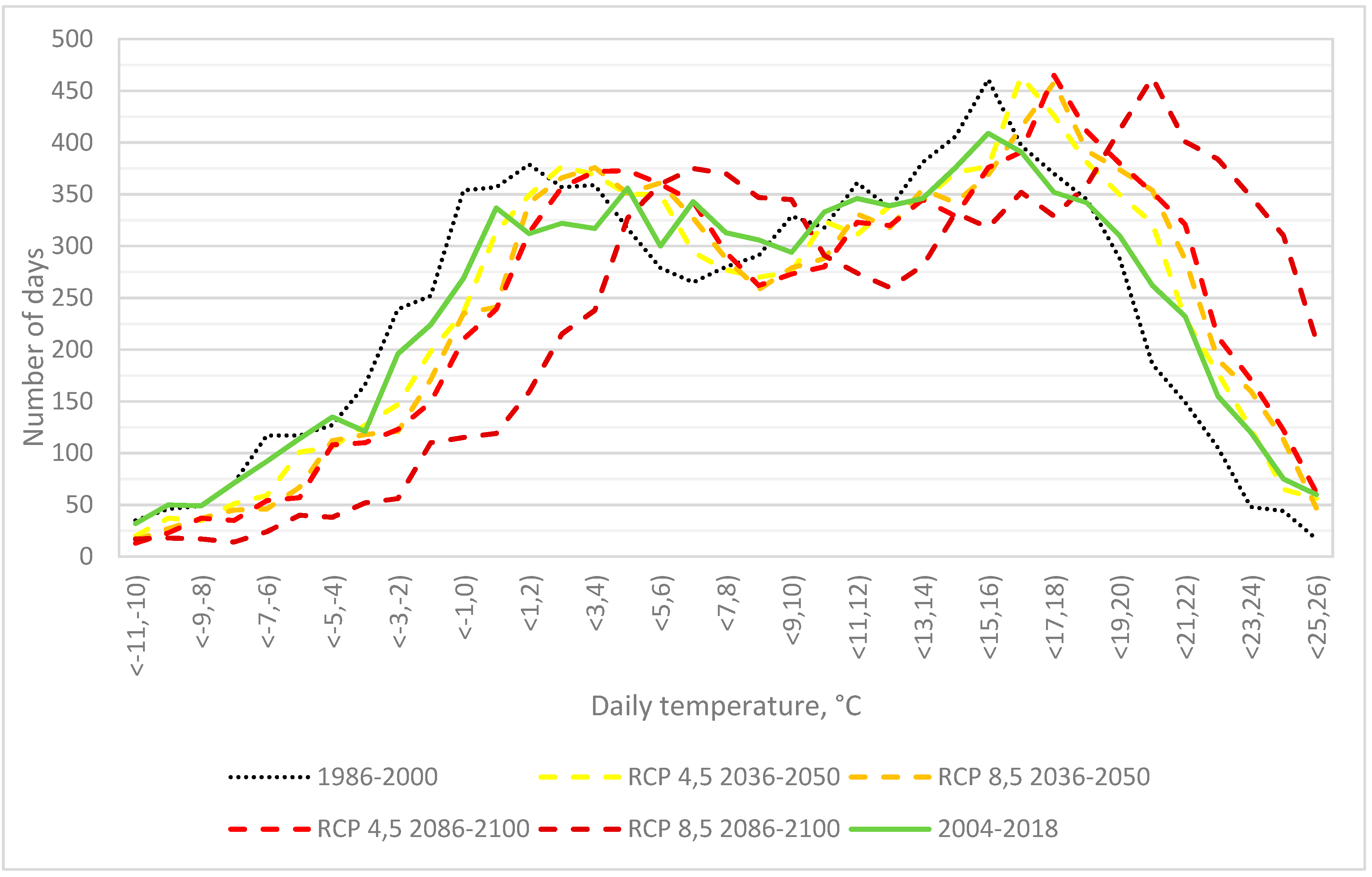
| Period: | 2036–2050 | 2086–2100 | ||
|---|---|---|---|---|
| Representative CO2 Concentration Scenarios: | RCP 4.5 | RCP 8.5 | RCP 4.5 | RCP 8.5 |
| Temperature increase Δti °C: | +1.5 | +2.1 | +2.4 | +5.3 |
| Ti | Temperature Range | dTi | nTi | λTi |
|---|---|---|---|---|
| °C | °C | - | - | number of failures/day at Ti temperature |
| −10.5 | <−11;−10) | 32 | 24 | 0.75 |
| −9.5 | <−10;−9) | 50 | 45 | 0.90 |
| −8.5 | <−9;−8) | 49 | 36 | 0.73 |
| −7.5 | <−8;−7) | 71 | 47 | 0.66 |
| −6.5 | <−7;−6) | 92 | 80 | 0.87 |
| −5.5 | <−6;−5) | 114 | 67 | 0.59 |
| −4.5 | <−5;−4) | 135 | 93 | 0.69 |
| −3.5 | <−4;−3) | 121 | 86 | 0.71 |
| −2.5 | <−3;−2) | 196 | 135 | 0.69 |
| −1.5 | <−2;−1) | 224 | 156 | 0.70 |
| −0.5 | <−1;0) | 269 | 198 | 0.74 |
| 0.5 | <0;1) | 337 | 190 | 0.56 |
| 1.5 | <1;2) | 312 | 182 | 0.58 |
| 2.5 | <2;3) | 322 | 187 | 0.58 |
| 3.5 | <3;4) | 317 | 170 | 0.54 |
| 4.5 | <4;5) | 356 | 178 | 0.50 |
| 5.5 | <5;6) | 300 | 157 | 0.52 |
| 6.5 | <6;7) | 343 | 158 | 0.46 |
| 7.5 | <7;8) | 313 | 150 | 0.48 |
| 8.5 | <8;9) | 306 | 123 | 0.40 |
| 9.5 | <9;10) | 294 | 131 | 0.45 |
| 10.5 | <10;11) | 333 | 104 | 0.31 |
| 11.5 | <11;12) | 346 | 143 | 0.41 |
| 12.5 | <12;13) | 339 | 116 | 0.34 |
| 13.5 | <13;14) | 346 | 140 | 0.40 |
| 14.5 | <14;15) | 376 | 153 | 0.41 |
| 15.5 | <15;16) | 409 | 171 | 0.42 |
| 16.5 | <16;17) | 391 | 157 | 0.40 |
| 17.5 | <17;18) | 352 | 163 | 0.46 |
| 18.5 | <18;19) | 342 | 144 | 0.42 |
| 19.5 | <19;20) | 310 | 136 | 0.44 |
| 20.5 | <20;21) | 262 | 109 | 0.42 |
| 21.5 | <21;22) | 232 | 108 | 0.47 |
| 22.5 | <22;23) | 155 | 63 | 0.41 |
| 23.5 | <23;24) | 120 | 65 | 0.54 |
| 24.5 | <24;25) | 75 | 37 | 0.49 |
| 25.5 | <25;26) | 60 | 30 | 0.50 |
| Ti | Temperature Range | λ% | λTiH | Number of Failures |
|---|---|---|---|---|
| °C | °C | - | number of failures/day at Ti temperature | - |
| −10.5 | <−11;−10) | 0.52 | 0.39 | 9 |
| −9.5 | <−10;−9) | 0.51 | 0.46 | 21 |
| −8.5 | <−9;−8) | 0.51 | 0.37 | 13 |
| −7.5 | <−8;−7) | 0.50 | 0.33 | 15 |
| −6.5 | <−7;−6) | 0.49 | 0.43 | 34 |
| −5.5 | <−6;−5) | 0.48 | 0.28 | 19 |
| −4.5 | <−5;−4) | 0.47 | 0.33 | 30 |
| −3.5 | <−4;−3) | 0.47 | 0.33 | 28 |
| −2.5 | <−3;−2) | 0.46 | 0.31 | 42 |
| −1.5 | <−2;−1) | 0.45 | 0.31 | 49 |
| −0.5 | <−1;0) | 0.44 | 0.32 | 64 |
| 0.5 | <0;1) | 0.43 | 0.24 | 46 |
| 1.5 | <1;2) | 0.42 | 0.24 | 44 |
| 2.5 | <2;3) | 0.41 | 0.24 | 44 |
| 3.5 | <3;4) | 0.40 | 0.21 | 36 |
| 4.5 | <4;5) | 0.39 | 0.19 | 34 |
| 5.5 | <5;6) | 0.38 | 0.20 | 31 |
| 6.5 | <6;7) | 0.36 | 0.17 | 26 |
| 7.5 | <7;8) | 0.35 | 0.17 | 25 |
| 8.5 | <8;9) | 0.34 | 0.14 | 17 |
| 9.5 | <9;10) | 0.32 | 0.14 | 19 |
| 10.5 | <10;11) | 0.31 | 0.10 | 10 |
| 11.5 | <11;12) | 0.30 | 0.12 | 18 |
| 12.5 | <12;13) | 0.28 | 0.10 | 11 |
| 13.5 | <13;14) | 0.27 | 0.11 | 15 |
| 14.5 | <14;15) | 0.25 | 0.10 | 15 |
| 15.5 | <15;16) | 0.23 | 0.10 | 17 |
| 16.5 | <16;17) | 0.21 | 0.09 | 13 |
| 17.5 | <17;18) | 0.19 | 0.09 | 15 |
| 18.5 | <18;19) | 0.17 | 0.07 | 11 |
| 19.5 | <19;20) | 0.15 | 0.07 | 9 |
| 20.5 | <20;21) | 0.13 | 0.05 | 6 |
| 21.5 | <21;22) | 0.11 | 0.05 | 5 |
| 22.5 | <22;23) | 0.08 | 0.03 | 2 |
| 23.5 | <23;24) | 0.06 | 0.03 | 2 |
| 24.5 | <24;25) | 0.03 | 0.01 | 1 |
| 25.5 | <25;26) | 0.00 | 0.00 | 0 |
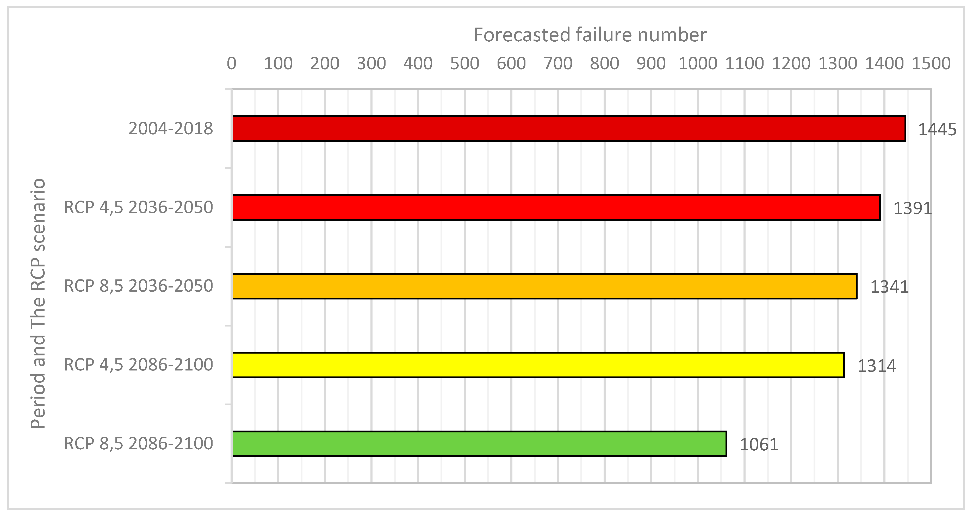
| ∑: | 1445 |
| Ti | Temp. Range | Number of Days | λTiH | Number of Failures | ||||||
|---|---|---|---|---|---|---|---|---|---|---|
| 2036–2050 | 2086–2100 | 2036–2050 | 2086–2100 | |||||||
| °C | °C | RCP 4.5 | RCP 8.5 | RCP 4.5 | RCP 8.5 | Number of Failures/ Day at Ti Temperature | RCP 4.5 | RCP 8.5 | RCP 4.5 | RCP 8.5 |
| −10.5 | <−11;−10) | 20 | 16 | 13 | 17 | 0.39 | 8 | 6 | 5 | 7 |
| −9.5 | <−10;−9) | 37 | 27 | 23 | 18 | 0.46 | 17 | 12 | 11 | 8 |
| −8.5 | <−9;−8) | 35 | 37 | 37 | 17 | 0.37 | 13 | 14 | 14 | 6 |
| −7.5 | <−8;−7) | 51 | 45 | 35 | 14 | 0.33 | 17 | 15 | 12 | 5 |
| −6.5 | <−7;−6) | 59 | 46 | 54 | 24 | 0.43 | 25 | 20 | 23 | 10 |
| −5.5 | <−6;−5) | 101 | 67 | 57 | 40 | 0.28 | 29 | 19 | 16 | 11 |
| −4.5 | <−5;−4) | 106 | 112 | 108 | 38 | 0.33 | 35 | 37 | 35 | 12 |
| −3.5 | <−4;−3) | 127 | 118 | 110 | 52 | 0.33 | 42 | 39 | 36 | 17 |
| −2.5 | <−3;−2) | 147 | 121 | 123 | 56 | 0.31 | 46 | 38 | 39 | 18 |
| −1.5 | <−2;−1) | 198 | 171 | 149 | 110 | 0.31 | 62 | 53 | 46 | 34 |
| −0.5 | <−1;0) | 236 | 235 | 210 | 115 | 0.32 | 76 | 76 | 68 | 37 |
| 0.5 | <0;1) | 314 | 241 | 239 | 119 | 0.24 | 76 | 58 | 58 | 29 |
| 1.5 | <1;2) | 349 | 342 | 313 | 159 | 0.24 | 85 | 84 | 77 | 39 |
| 2.5 | <2;3) | 377 | 366 | 357 | 215 | 0.24 | 89 | 87 | 85 | 51 |
| 3.5 | <3;4) | 369 | 376 | 372 | 238 | 0.21 | 79 | 80 | 79 | 51 |
| 4.5 | <4;5) | 350 | 351 | 373 | 327 | 0.19 | 68 | 68 | 72 | 63 |
| 5.5 | <5;6) | 350 | 361 | 360 | 360 | 0.20 | 69 | 71 | 71 | 71 |
| 6.5 | <6;7) | 294 | 327 | 343 | 375 | 0.17 | 49 | 55 | 57 | 63 |
| 7.5 | <7;8) | 277 | 288 | 294 | 370 | 0.17 | 47 | 48 | 49 | 62 |
| 8.5 | <8;9) | 270 | 258 | 262 | 347 | 0.14 | 37 | 35 | 36 | 47 |
| 9.5 | <9;10) | 275 | 279 | 273 | 345 | 0.14 | 40 | 40 | 40 | 50 |
| 10.5 | <10;11) | 324 | 288 | 280 | 291 | 0.10 | 31 | 28 | 27 | 28 |
| 11.5 | <11;12) | 311 | 331 | 323 | 274 | 0.12 | 38 | 41 | 40 | 34 |
| 12.5 | <12;13) | 339 | 318 | 320 | 260 | 0.10 | 33 | 31 | 31 | 25 |
| 13.5 | <13;14) | 344 | 355 | 345 | 281 | 0.11 | 37 | 38 | 37 | 30 |
| 14.5 | <14;15) | 371 | 342 | 329 | 332 | 0.10 | 38 | 35 | 33 | 34 |
| 15.5 | <15;16) | 377 | 369 | 376 | 318 | 0.10 | 36 | 36 | 36 | 31 |
| 16.5 | <16;17) | 464 | 415 | 391 | 352 | 0.09 | 40 | 36 | 34 | 30 |
| 17.5 | <17;18) | 426 | 458 | 465 | 329 | 0.09 | 38 | 41 | 42 | 30 |
| 18.5 | <18;19) | 381 | 392 | 411 | 359 | 0.07 | 28 | 29 | 30 | 26 |
| 19.5 | <19;20) | 350 | 374 | 380 | 412 | 0.07 | 24 | 25 | 26 | 28 |
| 20.5 | <20;21) | 322 | 354 | 352 | 463 | 0.05 | 18 | 19 | 19 | 25 |
| 21.5 | <21;22) | 230 | 287 | 321 | 401 | 0.05 | 12 | 14 | 16 | 20 |
| 22.5 | <22;23) | 177 | 190 | 212 | 384 | 0.03 | 6 | 6 | 7 | 13 |
| 23.5 | <23;24) | 124 | 160 | 171 | 348 | 0.03 | 4 | 5 | 5 | 11 |
| 24.5 | <24;25) | 65 | 113 | 122 | 310 | 0.01 | 1 | 2 | 2 | 5 |
| 25.5 | <25;26) | 56 | 47 | 62 | 209 | 0.00 | 0 | 0 | 0 | 0 |
| ∑: | 1391 | 1341 | 1314 | 1061 | ||||||
| Period | 2036–2050 | 2086–2100 | ||
|---|---|---|---|---|
| Representative CO2 concentration scenarios | RCP 4.5 | RCP 8.5 | RCP 4.5 | RCP 8.5 |
| Change in the number of failures dependent from temperature change % | −3.74 | −7.20 | −9.07 | −26.57 |
| Total change in the number of failures % | −1.22 | −2.35 | −2.96 | −8.66 |
© 2019 by the authors. Licensee MDPI, Basel, Switzerland. This article is an open access article distributed under the terms and conditions of the Creative Commons Attribution (CC BY) license (http://creativecommons.org/licenses/by/4.0/).
Share and Cite
Żywiec, J.; Piegdoń, I.; Tchórzewska-Cieślak, B. Failure Analysis of the Water Supply Network in the Aspect of Climate Changes on the Example of the Central and Eastern Europe Region. Sustainability 2019, 11, 6886. https://0-doi-org.brum.beds.ac.uk/10.3390/su11246886
Żywiec J, Piegdoń I, Tchórzewska-Cieślak B. Failure Analysis of the Water Supply Network in the Aspect of Climate Changes on the Example of the Central and Eastern Europe Region. Sustainability. 2019; 11(24):6886. https://0-doi-org.brum.beds.ac.uk/10.3390/su11246886
Chicago/Turabian StyleŻywiec, Jakub, Izabela Piegdoń, and Barbara Tchórzewska-Cieślak. 2019. "Failure Analysis of the Water Supply Network in the Aspect of Climate Changes on the Example of the Central and Eastern Europe Region" Sustainability 11, no. 24: 6886. https://0-doi-org.brum.beds.ac.uk/10.3390/su11246886