Modelling Public Transport Accessibility with Monte Carlo Stochastic Simulations: A Case Study of Ostrava


1
Department of Geoinformatics, VSB-Technical University of Ostrava, 70800 Ostrava, Czech Republic
2
Department of Control Systems and Instrumentation, VSB-Technical University of Ostrava, 70800 Ostrava, Czech Republic
3
Department of Geoinformatics, Palacky University Olomouc, 77147 Olomouc, Czech Republic
*
Author to whom correspondence should be addressed.
Sustainability 2019, 11(24), 7098; https://0-doi-org.brum.beds.ac.uk/10.3390/su11247098
Submission received: 5 November 2019
/
Revised: 2 December 2019
/
Accepted: 7 December 2019
/
Published: 11 December 2019
(This article belongs to the Special Issue Advanced Travel Demand Modelling for Sustainable Transportation)
Abstract
:Activity-based micro-scale simulation models for transport modelling provide better evaluations of public transport accessibility, enabling researchers to overcome the shortage of reliable real-world data. Current simulation systems face simplifications of personal behaviour, zonal patterns, non-optimisation of public transport trips (choice of the fastest option only), and do not work with real targets and their characteristics. The new TRAMsim system uses a Monte Carlo approach, which evaluates all possible public transport and walking origin–destination (O–D) trips for k-nearest stops within a given time interval, and selects appropriate variants according to the expected scenarios and parameters derived from local surveys. For the city of Ostrava, Czechia, two commuting models were compared based on simulated movements to reach (a) randomly selected large employers and (b) proportionally selected employers using an appropriate distance–decay impedance function derived from various combinations of conditions. The validation of these models confirms the relevance of the proportional gravity-based model. Multidimensional evaluation of the potential accessibility of employers elucidates issues in several localities, including a high number of transfers, high total commuting time, low variety of accessible employers and high pedestrian mode usage. The transport accessibility evaluation based on synthetic trips offers an improved understanding of local situations and helps to assess the impact of planned changes.
1. Introduction
Increasing traffic is an inherent symptom of vigorous urban development and its prosperity, but is concurrently one of the main factors that contribute to the deterioration of the urban environment and the endangerment of the sustainability of urban development. Public transport (PT) represents the main sustainable mode of urban mobility [1] and improves social equity and cohesion. In many countries, PT continues to represent an important share of transport, especially in cities.
Local governments aim to improve PT’s utilisation and attractiveness to decrease the volume of individual car transport and to motivate people to shift their transport modes towards more environmentally friendly means. Many empirical studies (e.g., [2,3,4,5,6,7]) help to discern which local factors influence PT usage and which advantages and impedances shape the behaviour of commuters. Ingrained habits and social perceptions play a larger role than economic reasons, and a coherent urban transport policy must be applied to achieve increased PT usage [8]. Moreover, increasing usage of PT is determined by the improvement of PT performance and quality, as well as by increasing opportunities around PT infrastructure [8].
Transport modelling not only enables an understanding of current transport flow and a prediction of the impact of envisaged changes, but also plays an essential role in accessibility modelling as part of more complex analyses. Corresponding to an increased interest in person-based accessibility modelling [9] and the development of intelligent transport systems, a paradigmatic shift from aggregated models, with the Four-Step Model (FSM) as the most prominent example [10,11], to activity-based and micro-scale models, can be observed [12].
Micro-scale models require fine-grained spatial interaction data. These may be obtained from zonal models using disaggregation methods, or from individual-level models based on activity–travel data [7,13,14]. Among many frameworks supporting disaggregated modelling for traffic planning, the following examples can be found: RAMBLAS [15], ALBATROSS [16], ILUTE [17], ILUMASS [18], SUMO [19]), TRANSIMS [20], SACSIM [21] and MATSIM [19].
Zonal aggregated models usually fail to accurately evaluate short-distance inter-zonal commutes and conditions for non-frequent groups of commuters [10,22], while individual models suffer from a lack of data ([23,24]). Benenson et al. [25] call for high-resolution analysis of PT accessibility, due to the high variability of accessibility results in the majority of Traffic Analysis Zones (TAZ), usually as a result of the penalizing effects of walking and waiting time on transit ridership.
The journey to work represents one of the most important day-to-day movements of economically active persons. Additionally, some authors consider the accessibility of jobs as a general measure of urban opportunity (accessibility of a destination of interest) [26,27]. To analyse personal commuting conditions, the ideal situation includes knowing the exact locations of one’s residence and regular workplace (or workplaces), and one’s relevant personal characteristics. However, such address-specific data are rarely available. The Social Statistics Data Warehouse of Statistics, Finland, offers dwelling coordinates and workplace coordinates for citizens, along with information on a variety of demographic features. The workplace coordinate coverage was 91% of all inhabitants in 2011 [28]. In Ireland, POWCAR data were collected as a part of the 2006 Irish Census, where almost all workplace locations for employed persons were geocoded [22]. Unfortunately, in Czechia, as well as in the majority of countries, there is no such available administrative evidence of workplaces for any given worker. Generally, in such cases, approximate data are used for the analysis, mainly Volunteered Geographical Information (VGI), mobile operator data, traffic smart card records (e.g., [29]), and surveys. Although such sources provide important knowledge, they are also limited by some technical issues, which are exemplified in the following paragraphs.
VGI [30,31,32] provides a good opportunity to collect a huge volume of individual routes with a series of space and time coordinates [33]. The collection consists of data from human sensors, where three key conditions must be met: technical ability (ownership of smart phones, smart watches, tablets or other wearables equipped with GPS receivers and appropriate software), knowledge (people acquainted with this technology), and motivation (people willing to upload and share these data, due to altruism, benefits etc. [34]). The satisfaction of these requirements generates a selectivity issue, because all social strata fail to be penetrated equally. In the dataset, the share of elderly and low-income persons, and persons unfamiliar with modern information and communication technologies may be underestimated. Additionally, a reduction in this selectivity bias is critical, due to the increased importance of PT for low-income groups [35,36]. Simultaneously, income shortages within these groups may impede the availability of the latest communications equipment, thus causing the selectivity issue to be that much more important for PT accessibility analysis than it is for other applications of VGI [37].
Another popular data source for mobility studies is datasets from mobile operators [38,39,40,41]. These datasets are usually based on Call Detail Records (CDRs), which contain the user’s ID, ID of the Base Transceiver Station (BTS), and date and time of active usage of a mobile phone. However, they are typically not provided in the form of individual route records due to privacy protection, but as the sum of CDRs aggregated into cells of certain points in time. The strengths of such data lie in their quantity and fine temporal resolution; nevertheless, the main issue for commuting analyses is the missing link between the individual properties of phone carriers and the purpose of their mobility. Mobility motivation is generally judged only from temporal behaviour, and therefore lacks clarity. Furthermore, the following constraints should be taken into account: missing information about the full route, limited data availability due to high costs and other restrictions, real data from one mobile operator and estimated data from other operators, only currently active SIM cards being recorded, difficulties eliminating robots and non-authorised access to mobile phones, limited spatial resolution due to the size of cells, and cell balancing.
On the other hand, questionnaires and interviews where socio-demographic characteristics, including travel behaviour and travel purposes, are recorded may provide a more comprehensive dataset. They offer a deep understanding by means of thorough characterisation of individual social and economic status, car ownership, income, preferences, family conditions, pro-environmental behaviour, etc. Travel behaviour is also influenced by a person’s system of values, e.g., postmodernist values, their relationship to environmental awareness (including perception of congestion, and perception of pollution), and how these are reflected in pro-environmental behaviour [42]. City-wide or regional interviews typically produce small datasets, vis-à-vis representative samples for each individual group of people. Thus, it is difficult to make inferences for small localities and assess the local transport situation using these data.
The evaluation of PT conditions is more complicated than the evaluation of individual car transport (ICT). Under ordinary conditions (e.g., no congestion), various metrics of ICT (e.g., travel time, distance, cost, fuel) are highly correlated; therefore, it may be enough to use any one of them to analyse commuting conditions [43]. The situation for PT is different and requires person-based accessibility measures to address the many person-related constraints and preferences [44]. There are many factors that can act as substantive impedances for PT usage, namely travel time, cost, walking distance, and waiting time, and usually they are not correlated simply. Furthermore, PT travel conditions may differ significantly on the outbound and return trips and thus require evaluation as a round trip [45].
To summarise, many difficulties are faced in obtaining and utilising large, unbiased representative datasets on human movements. We can substitute such datasets by utilising simulations of human behaviour following certain models with an appropriate stochastic component, which implements the variability and uncertainty of conditions including, but not always, the rational behaviour of real commuters.
To overcome these issues, a new, micro-scale, Monte Carlo simulation-based model for evaluation of local commuting conditions and potential accessibility is introduced. The aim of this paper is to highlight some specific features of the system, such as the utilisation of personal characteristics, activity-driven modelling (i.e., chaining of activities with fixed and soft temporal intervals or starts), and optimised PT trips selected from the full set of possibilities within the given time interval and k-nearest stops according to several criteria, as well as a discrete choice of targets, and implementation into the distributed client-server software enabling large computations.
The paper is organised as follows: the first section gives an overview of related works, underlining some existing limitations. The second section summarises the outputs of the travel survey in Ostrava. The third section presents the design of the simulation model. The fourth section describes the implementation of the modelling system and settings for alternative models. The fifth section provides a validation of the models. The sixth section presents the results of potential accessibility modelling in Ostrava. The discussion and conclusions summarise the main features of the introduced modelling approach and provide a comparison to existing systems.
2. State-of-the-Art
2.1. Microsimulation Modelling
Stochastic microsimulations of activity patterns can be based on different principles, and are currently dominated by agent-based modelling (ABM). ABM controls the behaviour of agents with a set of rules, the status of agents and external stimuli, which enables their coordination and interaction, which is useful for the integration of social behaviour and building dynamic systems. The disadvantages of ABM lie in the complexity of the systems and subjective choices, but also in performance limitations [46] and dealing with space [47]. Microsimulation modelling may reach the level of individual persons and vehicles. Usually, ABM is focused on individual vehicle modelling, while PT modelling remains a minor topic. The following examples demonstrate the development of this type of modelling and the level reached, and also comment on their simplifications and accompanying issues.
One of the first microsimulation models was RAMBLAS [15], which simulated daily activity patterns for regional planning in the Eindhoven region (NL). A synthetic population based on Monte Carlo simulations and activity agendas randomly drawn from the national distribution were used [44]. It was focused only on individual vehicle transport.
The ILUMASS project [18] integrated an activity-based simulation model of urban traffic flows, and a microscale ABM of household and firm development, to obtain the resulting changes in land and housing markets and the environmental impacts. Sub-models were connected via files that caused excessive computing times and limited operational usage [48].
Lovelace et al. [49] used a microsimulation of individual commutes to the nearest employment centre. The model was optimised to minimise differences between simulation results and census data. Simulated origin–destination (O–D) pairs were aggregated to display travel patterns and evaluate distances to employment centres, as well as to identify important destinations, etc. However, only driving and walking transport modes were modelled.
Greulich et al. [50] developed a multimodal ABM with a flexible framework where individual agents could reschedule their trips when unexpected events occurred. Another multimodal transport model was developed by Dobler and Lämmel [51]. Their hybrid approach enabled the combination of macro-scaled demand models with micro-scaled, force-based, and agent-based models, where the latter was meant to represent active modes of transport (walking, cycling) [12].
One of the most rapidly developing projects, MATSim, provides a modular framework to implement large-scale, agent-based transport simulations. MATSim includes demand modelling, agent-based mobility simulations, iterative processing to reach an optimum model, and methods to analyse the outputs [19]. MATSim was implemented in numerous studies [52], i.e., for an accessibility evaluation in the Metropolitan area of Zurich [53], travel behaviour under the condition of limited available survey data in China [54], transport energy demand modelling in Croatia [55], and cordon toll policy using mobile phone records in Barcelona [41]. While, at the beginning, the microsimulation was focused on the driving mode, recent development has enabled PT modelling (detection of frequent transfer locations in Seoul [56], PT accessibility for Singapore [57], locating transport facilities [58], and a comparison of fixed and flexible PT [59]) and new modes such as carsharing (e.g., the impact of parking price policy on free-floating carsharing in Zurich [60]) or autonomous vehicles (e.g., transport policy optimisation for autonomous vehicles in Zug [61]). Accessibility studies using MATSim vary in employed datasets, travel modes and focus. For the evaluation of PT, typically no time restrictions or temporal variability were taken into account. The missing temporal changes and neglected variability in schedules were also criticised by Zhang et al. [62].
Liu and Zhou [63] applied ABM for modelling capacity-constrained transit service, though no personal preferences or social behaviour were utilised in this model.
Social behaviour (e.g., job competition) was included in the ABM model by Huang [44]. Another advantage of his model was the integration of schedules with anticipated delays. Nevertheless, he simplified the model to include only job opportunities within a fixed Euclidean walking distance of 1 km, and neither real employers nor residential locations were taken into account. Personal behaviour was deduced from the national census data using a one-size-fits-all approach.
ABM is not the only approach to microsimulation modelling. Hybrid models represent a combination of aggregated and disaggregated models. The IRPUD model [48] is a dynamic simulation model of intraregional locations and mobility decisions in an urban region where the travel behaviour of individual households is modelled at a zonal level. It was used to simulate scenarios of fuel price increases and different combinations of activities and policies. As part of the solution, they modelled job accessibility in the Dortmund region, but only for individual transport.
2.2. Zonal Model Considerations
The classic modelling concept is usually based on four-step modelling (FSM) [11]. In FSM, zonal tessellation (usually TAZ) of the area is applied, and the simulated trips are distributed equally over the whole study area. A comprehensive overview of different transport models and approaches was provided by Ortúzar and Willumsen [10]. If the origin–destination matrices are built for zones and not for locations, it can provide only general spatial information [12], which limits the usage of address-based specific information, but, conversely, makes it simpler to model spatial interactions using, e.g., gravity models. Except for gravity models, discrete-choice models play an important role in the improved utilisation of observed individual choices. These models interpret more influential variables than gravity models, enabling better adaptation [64]. However, discrete-choice models are unable to integrate different sizes and attractiveness of individual targets, as opposed to what is available with gravity models using generalised distance–decay functions (e.g., [27]), sometimes also combined with a Huff model ([65,66,67]). Both models are based on zones, typically TAZ ([7,68]). A common shortcoming of zonal models is that they cannot fully utilise individual point-based targets and their properties, such as location, capacity, and time window and constraints, to improve the accuracy of transport modelling.
3. Survey Results in Ostrava
3.1. Study Area
The model was tested and evaluated for Ostrava, the centre of the Moravian–Silesian region situated in northeastern Czechia. The Ostrava XXL PT zone (Ostrava PT greater zone) has 401,000 inhabitants (2015) and an area of 530 km2. The urban PT network consists of 531 stops and 81 routes (bus, tram, and trolleybus) operating around 7150 trips on any given weekday.
In 2014, a questionnaire was conducted by a group of university researchers, including the authors of this paper, in order to understand the travel behaviour of respondents and their travel diaries. The respondents were asked to describe their usual daily trips based on starting and ending points, trip duration, means of transport used, purpose, and frequency. The total number of questionnaires completed was 534 (0.2% of the population, which is not high, and makes it difficult to draw firm conclusions). The Pencil And Paper Interview (PAPI) method was applied, and the sampling quota of respondents was stratified according to gender, age and education level [69]. The city was divided into 13 zones to ensure an even territorial distribution of respondents. The main class of respondents was full-time workers (46%), followed by retirees (20%), students (17%), self-employed (7%), persons on parental leave (6%) and unemployed (5%). The composition of the sample corresponded to the distribution of the general population by gender (male 48%), age (14% in 15–24, 67% in 25–64, 19% in 65+), and highest achieved level of education (tertiary 23%, secondary with graduation 39% and 28% without graduation, primary 10%). The deviation from the required stratification was below 1% for gender and age categories. The places of residence, origins, and destinations of all trips on weekdays and weekends (a total of 9959 points) were geocoded using Google Geocoding API [70].
The survey results were aggregated according to the following population groups: retired, employed, self-employed, unemployed, and students. The frequency analysis of recorded trips provided a quantitative assessment of group priorities for travel purpose, destination, time, and transport mode.
A reconstruction of all day trips enabled the discovery of typical scenarios (Day Activity Pattern according to [10]), daily movements (Figure 1) and the temporal distribution of activities (Figure 2). The evaluation of these distributions is necessary to draw random samples during Monte Carlo stochastic simulations of trips, similar to, for example, the Portland model in [71]. Noticeably, the patterns reflect differences in working and non-working days, and in population groups (Figure 1). According to the survey results, three quarters of daily movements are simple return trips to one destination. This figure corresponds well to the 70% found in Auckland [10]. Almost 90% of workers’ daily activities on weekdays (WD) are related to work, including 11% of trip chains connecting working and shopping. Pensioners declared shopping as the most prominent activity both for weekdays and weekends (WK) (40–50%). Different activities on WD and on WK were reported by students. They declared almost 90% of daily activities to be linked with studies and only a small portion were combined with sport or shopping, while, on WK, they engaged mainly in sport, work or shopping. Visiting family and friends is a specific weekend activity for all groups, except for students.
The temporal distribution of the beginning of travel activities for employees (Figure 2) shows the dominant peak of commuting to work early in the morning on weekdays and the multimodal distribution of commuting to work during weekends, where work shifts are more noticeably imprinted in the pattern (13:00 h for the second shift and 21:00 h for the third shift). Bimodal distribution is typical for escorting family members, usually children, on weekdays. Sport is typically an afternoon activity, while shopping is indicated by a secondary small peak in the morning hours for employees on non-working days, rather than before work.
3.2. Distance–Decay Impedance Functions
A profound understanding of trip distribution and the calibration of gravity models requires a distance–decay function (DDF) evaluation. These functions are represented by the relative distribution functions of travel distance and travel time constructed in the case of sufficient sample size for each combination of transport mode, purpose, personal economic activity, type of day and urban category (Figure 3a,b).
Differences between transport modes are clearly visible (Figure 3a). As expected, walking is limited to short distances and 90% of walks are shorter than 2 km. The cumulative distribution of urban PT trips continuously increases up to 8 km, which corresponds to the longest distances between borders of dense peripheral settlements and the city centre. Beyond this limit, distances grow rapidly, but such trips rarely occur. Driving is used for longer trips; the median is 6.4 km and the 9th decile is 13.7 km. The longest recorded car trip corresponds to the diameter of the study area.
Density of urbanisation (Figure 3b) also indicates a significant influence on the expected length of trip. Urban land cover categories include dense urbanised (city centre or compact settlement) and sparse urbanised (family houses, and mixed residential, commercial and industrial zones) settlements. However, few observations for sparse urbanised areas were recorded. It is clear that trip distances in dense urbanised areas are noticeably shorter (by approximately a third) than those for sparse urbanised areas, where suburbs are also included.
For all groups, various regression functions (i.e., exponential, power, Weibull, gamma, lognormal, and Box–Cox) were tested. Discussion on the behaviour and testing of such functions can be found in, e.g., [72,73,74]. In the majority of groups analysed, the best approximation was reached using the Weibull function [75] (Equation (1)):
where x stands for distance, and a and b are parameters for optimisation, with the approximate interpretation that a is more related to the scale of trips, while b corresponds to the shape of the function and variability of trip length. This function was used for approximation of all group DDFs; the differences lie only in the a and b parameters. DDFs characterise groups’ different perceptions of distance and willingness to travel. This same characterisation was applied in order to modify functions for travel time instead of distance. For the sake of simplicity, we did not adopt the name of the impedance function for, e.g., the temporal–decay function.
4. TRAMsim Simulation System
4.1. Concept of Modelling
The TRAMsim simulation system is based on the concept outlined in Figure 4 and is explained below. The simulation system is controlled by a set of parameters that should be fitted to the expected behaviour of the commuting community. The process of modelling is subdivided into the main four phases.
First, a population of interest is selected. It may represent a current resident population, population prediction or a selected category of person. The population choice influences the important parameter settings for simulations, including the number of simulations, maximal walking distance, number of proximal stops, description of chaining activities and related time settings (e.g., earliest time to leave home, latest time to return home, time tolerance, time interval requested before or after the activity, time distribution of activities). Important aspects of activities and behaviour have been explained in previous work ([10], p. 482). Within our concept, activities can be described as soft activities with unknown targets and unknown requested times, where only an activity type is known, or fixed activities where the target and/or requested time is known. For both soft and fixed activities, the potential set of targets is known, and each target is characterised by a precise location, size or capacity, and temporal restrictions.
After the population selection, the scenario is selected. The scenario consists of a chain of activities with a defined order. Each activity has an indicated minimal duration and may also have a fixed time plan (e.g., required starting time), which is suitable for work shifts, cultural and sporting events, etc.
Simulations for each origin begin with the search and evaluation of all possible transport connections within one hour (before and after) the planned activity to all destinations of the given type. The multithreading computing searches for connections between the specified number of stops closest to the origin and the destination. The search respects the parameters for the given type of simulation, scenario and personal features. If no connection is found, the time interval is extended sequentially by one hour.
Walking to and from stops is included as an obligatory part of each PT trip (similar to [25]). Furthermore, walking directly (hereafter referred to as pedestrian mode) between the origin and the destination is evaluated, which is important for shorter trips.
All found connections (D1a–Dnz) are compared, and, according to the personal/purpose travel optimality criterion (fastest, shortest, with minimum changes, random, latest, earliest), the most suitable trip from the given origin to each destination is selected (D1–Dz). In this way, the set of potential trips is reduced to one optimal trip from the given origin to each destination.
Next, the gravity value for each destination from the given origin is calculated. The gravity model utilises the size of the target, trip duration (including walking and waiting time) and the appropriate distance–decay impedance function. The DDF for modelling is selected according to the mode of transport, target categories, economic activities of the respective person, type of day, and category of the location. The resulting gravity value is obtained by multiplying the attractiveness by the target weight (Equation (2)):
where Gij stands for the gravity value, Aij is the attractiveness of the j-target from the i-origin, f() is the appropriate distance–decay impedance function, and tij is the travel time between i and j locations.
Gij = Aij * f(tij),
The attractiveness of a j-target is directly proportional to the size of the target, analogous to the Huff probability model [65,76]) for shopping gravity models, where the size of a target is typically expressed as the area of the given shop. It is calculated for the given type of person from the trip duration transformed by the DDF. The target size is a parameter that directly influences the size of the interaction; in the case of commuting to work, the number of employees is used [77].
The system currently implements three regimes of selection for the destination from the given origin from the full set of targets—fully random, maximal gravity and proportional gravity. Fully random selection utilises a uniform distribution, where each destination possesses the same probability of selection using a Monte Carlo drawing. Such an option may be a relevant alternative for small settlements where differences in distance can be neglected. The maximal gravity mode selects the target with the maximal gravity function value. This option is related to distance–decay utility maximisation [78] and assumes that everyone selects one’s job purely according to minimal travel impedance and maximal size of employer. Correspondingly, during simulations, the appropriate employer for each given origin is always selected. The proportional gravity mode intends to select targets proportionally to the distribution of the gravity value for all targets. It is implemented using a Monte Carlo drawing from the sum of the gravity values. All procedures are fully described in Appendix A.
By employing one of these selection options, one destination for the given origin is selected and one simulated trip is finished. Trip characteristics are recorded, including start time, finish time, travel time, total travel time (including walking), distance, number of changes, price, walking distance to/from the stop, and transport mode (public transport/walking). The simulations are repeated until the required number is reached, yielding large trip tables of person-commuting values.
The process can be iterated by selecting another possible scenario for the given population, or restarted by selecting another population (typically another person category).
4.2. TRAMsim Implementation
Simulations are performed in a system called TRAMsim. As was mentioned previously, the most frequent variants of simulation machines are ABM models. However, generally ABM models are not considered to be designed for extensive simulations [79]. In this case study, procedural modelling was preferred because of the massive extent of searching for PT connections and the requirements for parallel and distributed processing. The procedural modelling was based on the execution of a sequence of activities undertaken by the population. The simulation of behaviour for more persons or variants of individual behaviour, reflecting different conditions (changed randomly or systematically), are performed by repeated executions of the model, as is done with ABM. The heterogeneity of the environment is also implemented in a similar way to ABM.
Achieving results within a reasonable timeframe requires massive parallel data processing. A new parallel processing with an automatic extendable client–server system using a Microsoft SQL Server (MS SQL Server) was developed. The MS SQL Server is a relational database server developed by Microsoft and is used for the storage and maintenance of travel data and the programming of the application with a Transact-SQL language [80]. The three-layer model includes a central server, auxiliary local SQL servers and client PCs (Figure 5). Generation of the travel requirements is done using the local copy of the underlying data to eliminate any overloads of the central server. During the subsequent receipt of the results, the local server writes the results onto both servers. This method significantly reduces the load on the central server, which allows for an increase in the number of clients by a factor greater than 100. The programming code is stored in the supplementary file S1.
A database application generates random transport requests, according to the expected behaviours and parameters of the system. The transport requests are processed by the subsystem for the searching, evaluation and optimisation of PT connections. This subsystem utilises a DLL (Dynamic-link) library provided by CHAPS Ltd., the administrator of the National Information System on Regular Public Passenger Transport Timetables, to search for all possible PT connections in the PT time schedules. This enables a selection from the full set of trips based on different priorities in order to minimise travel time, distance, cost, number of transfers and waiting time within the given time period. The system distributes requests among a large number of clients and stores the results in the database server.
Currently, the system does not implement the uncertainty of transport timetables, due to congestion, for example. This is a result of the first implementation being done in Ostrava, where delays in PT are usually minimal and timetables are well respected (93% within a 3 min tolerance [81]).
4.3. TRAMsim Testing
For testing and validation, the simple Home–Workplace–Home scenario was implemented and analysed. Multipurpose trips were not included in the case study; however, the same model can be implemented to analyse trips of that nature. In TRAMsim, origin locations can be simulated, but currently they are substituted by fixed centres of small urban polygons. This corresponds to an intermediate approach in activity-based models [10]. The locations of residents (Home) were represented by 280 median centres of Basic Settlement Units (BSUs). The median centres were calculated using the distribution of address points in the given BSU representing a residential centre of the settlement unit.
Presently, the demand from any given origin was fixed to establish the same population demand for all localities, in order to not mirror the current population situation (number, structure), but, instead, a potential of accessibility. The number of demands from each location equals the number of simulations done for that location.
Instead of synthesising workplace locations inside a destination zone, current opportunities were mapped in sufficient detail and destinations were selected from the real set of localised targets using one of the destination-selection criteria (typically proportional gravity).
Contrary to other studies, (e.g., [7,44]), we mapped all significant workplaces (generally 50+ employees) in the pilot area (Ostrava + 20 km buffer), identified their locations as potential destinations, and estimated the number of employees as a basis for the evaluation of attractiveness. Various registries of employers and companies were explored for this purpose. The final set of workplaces was derived from the registry of the local labour office and was complemented by evidence from other sources (mainly the register of companies) and downscaled to cover all premises according to their relative size based on experts’ estimations. Such estimated values are obviously sources of uncertainty; nevertheless, they are used to calculate gravity values and do not represent constraints to limit the number of workers commuting to a given employer (no double constrained gravity model is applied). Optionally, work regimes (i.e., the start and end of a shift) can be recorded, similarly to other types of targets, where temporal constraints are recorded.
According to [82], the three stops nearest to the origin and the destination (nine combinations in total) were selected to search for various transport connections. In the following example, 977,760 O–D transport requests were processed and, for each request, about 25 connection variants were evaluated to find an optimal transport connection. Additionally, a pedestrian-mode trip between each origin and destination was evaluated.
4.4. Two Alternative Models for Testing
The number of PT stop combinations indicates a demanding computation, similar to other studies ([44,83,84]). The question is, is it necessary, or is it possible, to obtain similar results with substantially lower computational effort? Two alternative models were built, and their results were analysed. The two commuting models were designed based on simulated movements to (1) one hundred randomly selected large employers with more than 100 employees (the random-above-limit model, e.g., [85]) and (2) one hundred proportional gravity-selected employers. The first model is implemented much more simply than the second, because it does not require frequency analysis, optimisation of the DDF, or estimation of the weight of the target. It was assumed that elimination of the distance–decay effect within a city would have a negligible impact. In both models, the same settings were applied: departure from home after 16:15 h, 15 min anticipated preparatory time before work, eight hours work, and return home before 22:00 h. The latest travel connection before the requested arrival time was preferred in order to minimise waiting time. This meant that, if working hours started at 08:00 h, the connection prior to and closest to the optimal arrival time of 07:45 h was selected. The beginning of working hours was randomised from the most probable interval between 06:00 and 08:00 h, according to the survey results (Figure 2). The maximal walking distance to a PT stop was 5 km, so as not to strictly limit accessibility in peripheral villages.
Results of the models differ substantially from one another, including in the related accessibility evaluations. Differences in the distribution of individual values can be seen both in centrally situated BSUs, as well as in those in a peripheral position (Velka Polom in Figure 6 and Figure 7). The proportional gravity model provides a much lower mean and median, as well as a more homogeneous distribution and fewer outliers than the random-above-limit model for both BSUs (Figure 6). This is verified in the maps (Figure 7), where the random-above-limit model often selects quite distant targets, contrary to more compact selection in the proportional gravity model. It is necessary to validate both models and decide if the differences are significant.
4.5. Model Validation
The validation of both models is challenging because comprehensive information is necessary for the simulation of individual activities and is almost never available with a sufficient range [49]. Such models cannot conceptually be fully validated against data, due to mismatching in the granularity, and abundance of simulation outputs and traffic count data [86,87]. Wegener and Spiekermann [48] recommend combining the statistical calibration of models with expert judgement and plausibility analysis. In this case, the validation of models was based on the comparison between the simulation outputs and frequencies of each travel time reported in travel diaries aggregated by distribution functions. The only modification of the survey data was to exclude reported trips where targets were outside of Ostrava. For validation, both graphic and statistical tools were applied. The results (Figure 8) clearly show a significant deviation from the random-above-limit model, where the share of large trips is much higher than the distribution of time from the travel survey (notice the rounding of time values by respondents). On the other hand, the results of the proportional gravity model seem to coincide with the original data quite well (Figure 9).
A good correlation between the survey results and simulation outputs from the proportional gravity model was verified via statistical testing. Both datasets did not originate from the normal distribution (Kolmogorov–Smirnov and Shapiro–Wilk tests, p < 0.001). According to the results of the non-parametric tests, as well as the t-test (Table 1), the two distributions are equal and there is no significant difference. This confirms that the simulations based on the described proportional gravity model are realistic.
We can conclude, based on the random-above-limit model analysis, that the simplification of a simulation based only on a selection of large employers is not appropriate, even within a city.
5. Potential Accessibility Evaluation in Ostrava
The proportional gravity model was applied to evaluate potential accessibility in Ostrava using PT and walking for the granularity of BSUs. This analysis demonstrated the variability of outputs from microsimulation modelling, as well as their usefulness for understanding the underlying factors and thoroughly explaining observed differences in accessibility results.
Without the availability of an individual vehicle, it is possible to commute to some of the employers from every origin, but under highly variable conditions. During simulations, 94% of available employers were used as destinations for simulated commutes. This means that the remaining 6% of employers may be less accessible via PT, or they may be located in the “shadow” of a competing large employer located within very close proximity. The share of accessible workplaces from each origin exhibits significant differences in the supply of workplaces (Figure 10a). The locations with the richest variety of available employers (>70%) are in the centre of Ostrava, as well as in some fragmented zones around it. A comparison between the share of accessible workplaces and employers’ locations (black dots) shows clear differences in the pattern, indicating the importance of attractiveness and PT conditions within the evaluation. Peripheral parts of the city show an obviously lower supply of accessible employers, but again the situation is heterogeneous. A low supply of employers is recognised in Jistebnik (SW corner, 39%), in several municipalities on the west border (less than 60%, Zbyslavice, Čavisov, Horní Lhota) and in the northeast corner around Bohumín (less than 60%). The underlying reasons for this can be understood using Figure 10 and Figure 11.
Jistebnik has a low number of employers within the municipality and in nearby accessible surroundings, thus the local labour market does not create a sufficient labour demand. During simulations, due to poor PT conditions (e.g., many transfers, low frequency, long walking distance to a stop), local employers within walkable distance were frequently selected (confirmed by the high share of pedestrian mode trips—more than 20% in Figure 10b) or workers commuted to more distant employers under poor conditions (reference the extreme number of changes per day in Figure 11b). Surprisingly, in Jistebnik, the total travel time per day was not worse than in the majority of other BSUs, which is explained by a smoothing effect of the mean between results for local commuting (including the dominating pedestrian mode) and distant commuting.
Bohumín shows some similarities, such as the low variety of employers connected with a very high share of pedestrian mode use; however, it boasts good travel times and a low number of changes (Figure 11). These attributes reveal a very close commuting network (built with local urban PT and pedestrian modes), in which Bohumín creates its own sufficient labour market with minimal requirements for commuting to other parts of the Ostrava XXL zone.
Finally, municipalities on the western border of Ostrava XXL show a low usage of the pedestrian mode, which indicates the absence of local employers. However, PT conditions are good (comparable to other geographically similar locations), especially when considering an acceptable average number of changes.
It is possible to analyse the situation in other municipal areas (BSUs) by employing the same technique. A high incidence of pedestrian mode usage is not only found in the centre of Ostrava, where the high supply of local employers and slower PT in the densely urbanised area leads to a preference for walking, but also in the eastern BSUs, close to external employers in the nearby city of Havířov.
Several BSUs (e.g., Vřesina) offer a good variety of employers, but exhibit a poor average travel time and high number of changes. According to average travel time, a poor commute of more than 90 mins per day exists in some locations, including in several isolated zones (14 BSUs), mainly on the borders, which represent only 1% of the population. More surprisingly, however, the second worst category (60–90 min commute) covers not only the majority of suburban areas, but also some internal parts of the municipality of Ostrava. These areas include 54% of BSUs, with 51% of the population (almost 190,000 people). This reveals some troublesome commuting durations using PT, which can generally be attributed to more than one change per trip.
The results indicate locations within Ostrava with a potential for improvement in PT service. Results were not influenced by adaptation strategies of residents, including relocation for better access to employers and other facilities, using individual transport or some shared modes of transport, changes in employer due to poor accessibility, etc.
6. Discussion and Conclusions
Stochastic microscale simulation-based modelling offers a more thorough and detailed understanding of local commuting conditions and PT issues. Usually, studies in this area are based on schemes of evaluation of respondents’ opinions on travel conditions (e.g., the multidimensional Rasch model in [88]). Even though this represents a direct way to evaluate customer satisfaction, there are questions about how to reach objectively comparable commuting conditions. Synthetic data can substitute or supplement existing real-world data, respecting existing PT conditions, targets’ property constraints, and personal and opportunity factors. For accessibility studies, trip simulation provides the benefit of a multidimensional evaluation of local PT conditions, including an assessment of total travel time per day, number of changes, walking distance, waiting time, and the frequency of utilised stops or links [89].
This paper introduces a new approach to activity-based microsimulation modelling using stochastic Monte Carlo simulations to generate synthetic trips, and its implementation using the TRAMsim system. Three main outputs are presented: (1) a new concept of modelling and its implementation in TRAMsim, (2) the results of the testing and validation of two commuting models and (3) a potential accessibility evaluation of workplaces in Ostrava.
A key decision for modelling is the choice of a population of interest. It is possible to focus on specific groups within the population, and to analyse and predict accessibility specifically for them (e.g., [67] for children, youth and seniors). Personal characteristics are described in more detail than in other studies, where usually only income level and car ownership are documented. Characteristics are derived from a local travel survey. The population must be described in terms of location (spatial distribution), socioeconomic status, travel preferences and behaviour. Similar to discrete-choice models [10], observation of individuals is recommended. Specific outputs include a description of all important scenarios (daily activity patterns) with identified activities, the temporal distribution of these activities and optimised distance–decay impedance functions, corresponding to different purposes. The scenarios may consist of more than one activity, respect the opening hours of businesses, and consider the temporal variability of the attractiveness of the destination.
Activities are linked with a set of real-world targets equipped with real properties, i.e., the locations (coordinates) of all premises, temporal constraints and preferences, and sizes or capacities. Trip destinations are selected only from this set of targets, which enables the provision of a more accurate evaluation of travel. The selection of targets is managed by one of three options, the proportional gravity model being the validated model for Ostrava. In this system, PT trips always include walking, as complete door-to-door trips are evaluated.
All public transport connections are searched for not only for the closest stop from the origin or destination (a common setting in many other studies) but also for the predefined set of nearest stops, where all stop–stop combinations are evaluated. This is a commonly overlooked issue, even though, especially in dense urban environments, walking distances to various stops frequently differ only slightly, but the performance (transport frequencies, and available modes and links) may differ significantly. For example, Ivan [90] confirmed that only about 50% of transit users in our region use the closest stop.
As well as this, several options for the method of travel are available. Even though the majority of studies use only the fastest connection from the given departure time (e.g., [25]), this option is not preferred for all people and all purposes. Our model deals with a specified time interval and finds not just the fastest connection within this interval, but also the latest, the earliest, the shortest, a random and a “comfort” option. The “comfort” option is appropriate for travellers with disabilities, accompanying other persons, with luggage or shopping bags, etc. The last option should be preferred by passengers aiming to minimise waiting time before a fixed-start event. These variants enable a better simulation of passenger behaviour, based on their personal properties and purposes.
The model is implemented in TRAMsim, a database application with an automatic extensible client-server system suitable for massive parallel processing. TRAMsim simulates the selection of targets, searches for optimal transport connections and generates synthetic sets of probable trips, using both PT and pedestrian mode, optimised according to personal characteristics and detailed mapping of opportunities for activities.
Within the Ostrava case study, two models for commuting to work were tested. Comparison of the test results for these two models (random selection of a large employer, and proportional gravity selection from all employers) proved that the computational load during simulations cannot be decreased by the simplification of the model based on a random-above-limit approach, even within a city, and shows a good correspondence of the proportional gravity model to the survey results. This is a significantly positive result, as some other microsimulation studies have not succeeded in validation of their models (e.g., in [7], both gravity and discrete-choice models failed in validation).
The successfully validated proportional gravity model was used for simulations. Synthetic trips were employed for the mapping and evaluation of potential workplace accessibility in Ostrava.
Accessibility was evaluated with a set of selected indicators suitable for PT, including the share of accessible employers, pedestrian mode usage, total commuting time, and number of changes. The accessibility was evaluated for the Home–Work–Home scenario representing a full daily tour, including walking to/from stops and pedestrian mode. Thus, the total travel time includes all travel time, walking time and waiting time. The evaluation of such a daily travel time budget eliminates a common issue in PT accessibility studies, where outbound and return trips differ significantly. The low variety of employers found in simulations indicates a limited offer, usually related to restricted transport options, where only some requested targets are accessible. The pedestrian mode usage, combined with other indicators, is able to distinguish relatively closed local catchments with limited accessibility of distant destinations. A high number of changes indicates higher discomfort for travelers, which may impede PT usage for some groups of people. Such multidimensional evaluations enable a better rendering of the local situation, identify specific issues in some localities, and evaluate the impact of planned transport changes.
In this case study, potential accessibility was evaluated with a monotone demand and does not reflect the current local population. The reason for this is that models with a synthetic current population (e.g., [15,44]) evaluate the current accessibility conditions, but they conserve the existing population and results are influenced by a different structure of residents. For example, zones populated mainly by retirees may exhibit good accessibility, due to pensioners’ prioritised commuting needs, such as shops, when, in reality, that same zone may have inadequate accessibility to employers or other types of destinations. Another issue with this kind of modelling is how to properly evaluate sparsely populated areas or locations under development. In such situations, it is possible to synthesise a standardised or target population. Using the same standardised population for all tested locations would enable the mapping of potential accessibility unbiased by the current population and its profile. The main disadvantage of simulation modelling can be seen in the great requirement for fine-grade local data and computation loads. This a common weakness [48,83,84], which still impedes the operational usage of such tools. Spiekermann and Wegener [91,92] described theoretical, empirical, practical and ethical limits for increasing the resolution of these models. In the TRAMsim case study, the model does not try to capture the full complexity of relationships between the population, land use and transport to simulate traffic flows in the real world. The focus of the simulation is on accessibility studies with partly fixed conditions, which decreases the uncertainty of the modelling and the computational load.
Potential weaknesses of the TRAMsim model can be seen in several instances. TRAMsim is unable to model social interaction. No activity across household members nor redistribution of activities among members can be implemented in an automatic manner. The social behaviour of the synthetic persons is not included, because the current focus of the system is on the potential accessibility evaluation and, therefore, no interactivity of the current population is modelled, similar to job competition in multiagent systems in [44]. Also, the gravity potential is evaluated for each target independently, and no synergic effect (sojourns) for clusters or chains of targets can be utilised. Additionally, no travel time uncertainty or schedules (e.g., congestion) are implemented. For the presented case study, this is a marginal problem, due to the positive fact that PT in Ostrava currently exhibits only small delays in scheduled times.
TRAMsim offers inspiration for improvements in PT modelling, which may also be applied in other simulation systems to reach more accurate modelling results. Improved understanding of local PT issues helps to adapt PT policy, to decrease real inconveniences impeding the wider usage of PT, and to decrease transport stress in modern cities.
Supplementary Materials
The following are available online at https://0-www-mdpi-com.brum.beds.ac.uk/2071-1050/11/24/7098/s1, Software code S1: TRAMsimSourceCode.txt, Table S2: AverageEval.csv, Table S3: SimulatedTrips.csv, Table S4: metadata.txt.
Author Contributions
Conceptualisation, J.H.; Data curation, J.T. and D.F.; Formal analysis, J.H. and J.T.; Methodology, J.H. and D.F.; Software, D.F.; Validation, J.H.; Visualisation, J.T. and V.V.; Writing—original draft, J.H. and J.T.; Writing—review and editing, V.V.
Funding
This research was funded by the Czech Science Foundation, grant number 14-26831S “Spatial simulation modelling of accessibility” and the European Regional Development Fund in the Research Centre of Advanced Mechatronic Systems, No. CZ.02.1.01/0.0/0.0/16_019/0000867 within the Operational Programme Research, Development and Education.
Conflicts of Interest
The authors declare no conflict of interest. The funders had no role in the design of the study; in the collection, analyses, or interpretation of data; in the writing of the manuscript, or in the decision to publish the results.
Appendix A. Explanation of the Regimes of Selection for the Destination from the Given Origin
Let be a set of origins and be a set of destinations:
For each element of the set, O exists as an ordered set of destination elements that is ordered by the value of gravity function .
The function returns the gravitational value, which represents the gravity between origin and destination . The function is defined by:
where function returns the attraction of destination from origin , function is the appropriate distance–decay impedance (temporal-decay) function, and function returns the travel time between and locations.
For each element of the set O, there also exists an ordered subset of elements of set where the gravitation ratio is greater than the randomly determined level. Set is defined by:
where is the random number from a uniform distribution from interval , is the number of elements in set , and is the index of element of ordered set .
For random choice of destination from origin :
where is the number of set elements , and is the random number from a uniform distribution from interval .
For maximal gravity choice of destination from origin :
where is the number of set elements .
For proportional gravity choice of destination from origin :
References
- Chen, Y.; Bouferguene, A.; Li, H.X.; Liu, H.; Shen, Y.; Al-Hussein, M. Spatial gaps in urban public transport supply and demand from the perspective of sustainability. J. Clean. Prod. 2018, 195, 1237–1248. [Google Scholar] [CrossRef]
- Zhao, P. The Impact of the Built Environment on Individual Workers’ Commuting Behavior in Beijing. Int. J. Sustain. Transp. 2013, 7, 389–415. [Google Scholar] [CrossRef]
- Grengs, J. Nonwork Accessibility as a Social Equity Indicator. Int. J. Sustain. Transp. 2015, 9, 1–14. [Google Scholar] [CrossRef]
- Akar, G.; Chen, N.; Gordon, S.I. Influence of neighborhood types on trip distances: Spatial error models for Central Ohio. Int. J. Sustain. Transp. 2016, 10, 284–293. [Google Scholar] [CrossRef]
- Shannon, J. Beyond the Supermarket Solution: Linking Food Deserts, Neighborhood Context, and Everyday Mobility. Ann. Am. Assoc. Geogr. 2016, 106, 186–202. [Google Scholar] [CrossRef]
- Martin-Barroso, D.; Nunez-Serrano, J.A.; Velazquez, F.J. Firm heterogeneity and the accessibility of manufacturing firms to labour markets. J. Transp. Geogr. 2017, 60, 243–256. [Google Scholar] [CrossRef]
- Chacon-Hurtado, D.; Gkritza, K.; Fricker, J.D.; Yu, D.J. Exploring the role of worker income and workplace characteristics on the journey to work. Int. J. Sustain. Transp. 2019, 13, 553–566. [Google Scholar] [CrossRef]
- Kaufmann, V. Modal Practices: From the rationales behind car and public transport use to coherent transport policies. World Transp. Policy Pract. 2000, 2000, 8–17. [Google Scholar]
- Geurs, K.T.; van Wee, B. Accessibility evaluation of land-use and transport strategies: Review and research directions. J. Transp. Geogr. 2004, 12, 127–140. [Google Scholar] [CrossRef]
- De Dios Ortúzar, J.; Willumsen, L.G. Modeling Transport, 4th ed.; Wiley: Hoboken, NJ, USA, 2011; ISBN 978-0-470-76039-0. [Google Scholar]
- McNally, M.G. The four-step model. In Handbook of Transport Modelling; Elsevier: Amsterdam, The Netherlands, 2008; pp. 35–53. ISBN 0-08-045376-7. [Google Scholar]
- Loidl, M.; Wallentin, G.; Cyganski, R.; Graser, A.; Scholz, J.; Haslauer, E. GIS and Transport Modeling—Strengthening the Spatial Perspective. ISPRS Int. J. Geo Inf. 2016, 5, 84. [Google Scholar] [CrossRef] [Green Version]
- Niedzielski, M.A.; O’Kelly, M.E.; Boschmann, E.E. Synthesizing spatial interaction data for social science research: Validation and an investigation of spatial mismatch in Wichita, Kansas. Comput. Environ. URBAN Syst. 2015, 54, 204–218. [Google Scholar] [CrossRef]
- Schleith, D.; Horner, M.W. Commuting, Job Clusters, and Travel Burdens Analysis of Spatially and Socioeconomically Disaggregated Longitudinal Employer-Household Dynamics Data. Transp. Res. Rec. 2014, 2542, 19–27. [Google Scholar] [CrossRef]
- Veldhuisen, J.; Timmermans, H.; Kapoen, L. RAMBLAS: A regional planning model based on the microsimulation of daily activity travel patterns. Environ. Plan. Econ. SPACE 2000, 32, 427–443. [Google Scholar] [CrossRef]
- Arentze, T.; Timmermans, H. A learning-based transportation oriented simulation system. Transp. Res. PART B Methodol. 2004, 38, 613–633. [Google Scholar] [CrossRef]
- Salvini, P.; Miller, E.J. ILUTE: An Operational Prototype of a Comprehensive Microsimulation Model of Urban Systems. Netw. Spat. Econ. 2005, 5, 217–234. [Google Scholar] [CrossRef]
- Beckmann, K.J.; Brüggemann, U.; Gräfe, J.; Huber, F.; Meiners, H.; Mieth, P.; Moeckel, R.; Mühlhans, H.; Rindsfüser, G.; Schaub, H.; et al. ILUMASS: Integrated Land-Use Modelling and Transport System Simulation; Deutsches Zentrum für Luft und Raumfahrt: Berlin, Germany, 2007. [Google Scholar]
- Horni, A.; Nagel, K.; Axhausen, K.W. The Multi-Agent Transport Simulation MATSim; Ubiquity Press: London, UK, 2016; ISBN 978-1-909188-75-4. [Google Scholar]
- Lee, K.S.; Eom, J.K.; Moon, D. Applications of TRANSIMS in transportation: A literature review. In Proceedings of the 5th International Conference on Ambient Systems, Networks and Technologies (ANT-2014), 4th International Conference on Sustainable Energy Information Technology (SEIT-2014); Shakshuki, E., Yasar, A., Eds.; Elsevier Science BV: Amsterdam, The Netherlands, 2014; Volume 32, pp. 769–773. [Google Scholar]
- Bradley, M.; Bowman, J.L.; Griesenbeck, B. SACSIM: An applied activity-based model system with fine-level spatial and temporal resolution. J. Choice Model. 2010, 3, 5–31. [Google Scholar] [CrossRef] [Green Version]
- O’Kelly, M.E.; Niedzielski, M.A.; Gleeson, J. Spatial interaction models from Irish commuting data: Variations in trip length by occupation and gender. J. Geogr. Syst. 2012, 14, 357–387. [Google Scholar] [CrossRef]
- Kung, K.S.; Greco, K.; Sobolevsky, S.; Ratti, C. Exploring Universal Patterns in Human Home-Work Commuting from Mobile Phone Data. PLoS ONE 2014, 9, e96180. [Google Scholar] [CrossRef] [Green Version]
- McArthur, D.P.; Hong, J. Visualising where commuting cyclists travel using crowdsourced data. J. Transp. Geogr. 2019, 74, 233–241. [Google Scholar] [CrossRef]
- Benenson, I.; Ben-Elia, E.; Rofé, Y.; Geyzersky, D. The benefits of a high-resolution analysis of transit accessibility. Int. J. Geogr. Inf. Sci. 2017, 31, 213–236. [Google Scholar] [CrossRef]
- Ahlfeldt, G. If Alonso was right: Modeling accessibility and explaining the residential land gradient. J. Reg. Sci. 2011, 51, 318–338. [Google Scholar] [CrossRef]
- Merlin, L.A. A portrait of accessibility change for four US metropolitan areas. J. Transp. Land Use 2017, 10, 309–336. [Google Scholar] [CrossRef] [Green Version]
- Piela, P. Commuting time for every employed: Combining traffic sensors and many other data sources for population statistics. In Proceedings of the 7th Conference European Forum for Geostatistics, Krakow, Poland, 26–31 August 2014. [Google Scholar]
- Medina, S.A.O.; Erath, A. Estimating Dynamic Workplace Capacities by Means of Public Transport Smart Card Data and Household Travel Survey in Singapore. Transp. Res. Rec. 2013, 2344, 20–30. [Google Scholar] [CrossRef]
- Goodchild, M.F. Citizens as sensors: The world of volunteered geography. GeoJournal 2007, 69, 211–221. [Google Scholar] [CrossRef] [Green Version]
- Flanagin, A.J.; Metzger, M.J. The credibility of volunteered geographic information. GeoJournal 2008, 72, 137–148. [Google Scholar] [CrossRef]
- Karimi, H.A. Big Data: Techniques and Technologies in Geoinformatics; CRC Press: Boca Raton, FL, USA, 2017; ISBN 978-1-138-07319-7. [Google Scholar]
- Sui, D.Z.; Elwood, S.; Goodchild, M.F. Crowdsourcing Geographic Knowledge: Volunteered Geographic Information (VGI) in Theory and Practice; Springer: Dordrecht, The Netherlands; New York, NY, USA, 2013; ISBN 978-94-007-4586-5. [Google Scholar]
- Coleman, D.; Georgiadou, Y.; Labonte, J. Volunteered Geographic Information: The nature and motivation of produsers. Int. J. Spat. Data Infrastruct. Res. 2009, 4, 332–358. [Google Scholar]
- Currie, G. Quantifying spatial gaps in public transport supply based on social needs. J. Transp. Geogr. 2010, 18, 31–41. [Google Scholar] [CrossRef]
- Serulle, N.U.; Cirillo, C. Transportation needs of low income population: A policy analysis for the Washington D.C. metropolitan region. Public Transp. 2016, 8, 103–123. [Google Scholar] [CrossRef]
- Goodchild, M.F.; Li, L. Assuring the quality of volunteered geographic information. Spat. Stat. 2012, 1, 110–120. [Google Scholar] [CrossRef]
- Deville, P.; Linard, C.; Martin, S.; Gilbert, M.; Stevens, F.R.; Gaughan, A.E.; Blondel, V.D.; Tatem, A.J. Dynamic population mapping using mobile phone data. Proc. Natl. Acad. Sci. USA 2014, 111, 15888–15893. [Google Scholar] [CrossRef] [Green Version]
- Kubicek, P.; Konecny, M.; Stachon, Z.; Shen, J.; Herman, L.; Reznik, T.; Stanek, K.; Stampach, R.; Leitgeb, S. Population distribution modelling at fine spatio-temporal scale based on mobile phone data. Int. J. Digit. Earth 2019, 12, 1319–1340. [Google Scholar] [CrossRef]
- Novak, J.; Ahas, R.; Aasa, A.; Silm, S. Application of mobile phone location data in mapping of commuting patterns and functional regionalization: A pilot study of Estonia. J. Maps 2013, 9, 10–15. [Google Scholar] [CrossRef]
- Bassolas, A.; Ramasco, J.J.; Herranz, R.; Cantu-Ros, O.G. Mobile phone records to feed activity-based travel demand models: MATSim for studying a cordon toll policy in Barcelona. Transp. Res. Part A Policy Pract. 2019, 121, 56–74. [Google Scholar] [CrossRef] [Green Version]
- De las Heras-Rosas, C.J.; Herrera, J. Towards Sustainable Mobility through a Change in Values. Evidence in 12 European Countries. Sustainability 2019, 11, 4274. [Google Scholar] [CrossRef] [Green Version]
- Horák, J.; Burian, J.; Ivan, I.; Zajíčková, L.; Tesla, J.; Voženílek, V.; Fojtík, D.; Inspektor, T.; Rypka, M. Prostorové simulační modelování dopravní dostupnosti, 1st ed.; Geographica; Česká geografická společnost: Prague, Czech Republic, 2019; ISBN 978-80-907728-0-9. [Google Scholar]
- Huang, R. Simulating individual work trips for transit-facilitated accessibility study. Environ. Plan. B Urban Anal. City Sci. 2019, 46, 84–102. [Google Scholar] [CrossRef]
- Lei, T.L.; Church, R.L. Mapping transit-based access: Integrating GIS, routes and schedules. Int. J. Geogr. Inf. Sci. 2010, 24, 283–304. [Google Scholar] [CrossRef]
- Grigoryev, I. AnyLogic 7 in Three Days; Create Space Independent Publishing Platform: Scotts Valley, CA, USA, 2016; ISBN 978-1-5089-3374-8. [Google Scholar]
- Rapant, P. Space in multi-agent systems modelling spatial processes. ACTA Montan. SLOVACA 2007, 12, 84–97. [Google Scholar]
- Wegener, M.; Spiekermann, K. Multi-level urban models: Integration across space, time and policies. J. Transp. Land Use 2018, 11, 67–81. [Google Scholar] [CrossRef] [Green Version]
- Lovelace, R.; Ballas, D.; Watson, M. A spatial microsimulation approach for the analysis of commuter patterns: From individual to regional levels. J. Transp. Geogr. 2014, 34, 282–296. [Google Scholar] [CrossRef] [Green Version]
- Greulich, C.; Edelkamp, S.; Gath, M. Agent-Based Multimodal Transport Planning in Dynamic Environments. In Proceedings of the KI 2013: Advances in Artificial Intelligence; Timm, I.J., Thimm, M., Eds.; Springer: Berlin/Heidelberg, Germany, 2013; pp. 74–85. [Google Scholar]
- Dobler, C.; Lämmel, G. Integration of a Multi-modal Simulation Module into a Framework for Large-Scale Transport Systems Simulation. In Pedestrian and Evacuation Dynamics 2012; Weidmann, U., Kirsch, U., Schreckenberg, M., Eds.; Springer International Publishing: Cham, UK, 2014; pp. 739–754. ISBN 978-3-319-02446-2. [Google Scholar]
- Axhausen, K.W. MATSim: An Update on Recent Work; ETH Zürich: Zürich, Switzerland, 2018. [Google Scholar]
- Floetteroed, G.; Chen, Y.; Nagel, K. Behavioral Calibration and Analysis of a Large-Scale Travel Microsimulation. Netw. Spat. Econ. 2012, 12, 481–502. [Google Scholar] [CrossRef]
- Zhuge, C.; Shao, C.; Gao, J.; Meng, M.; Xu, W. An Initial Implementation of Multiagent Simulation of Travel Behavior for a Medium-Sized City in China. Math. Probl. Eng. 2014. [Google Scholar] [CrossRef]
- Novosel, T.; Perkovic, L.; Ban, M.; Keko, H.; Puksec, T.; Krajacic, G.; Duic, N. Agent based modelling and energy planning - Utilization of MATSim for transport energy demand modelling. Energy 2015, 92, 466–475. [Google Scholar] [CrossRef] [Green Version]
- Ali, A.; Kim, J.; Lee, S. Travel behavior analysis using smart card data. KSCE J. Civ. Eng. 2016, 20, 1532–1539. [Google Scholar] [CrossRef]
- Van Eggermond, M.A.B.; Erath, A. Pedestrian and transit accessibility on a micro level: Results and challenges. J. Transp. Land Use 2016, 9, 127–143. [Google Scholar] [CrossRef] [Green Version]
- Zhuge, C.; Shao, C. Agent-Based Modelling of Locating Public Transport Facilities for Conventional and Electric Vehicles. Netw. Spat. Econ. 2018, 18, 875–908. [Google Scholar] [CrossRef]
- Narayan, J.; Cats, O.; Van Oort, N.; Hoogendoorn, S. Performance assessment of fixed and flexible public transport in a multi agent simulation framework. In Proceedings of the 20th Euro Working Group on Transportation Meeting, EWGT 2017, Budapest, Hungary, 4–6 September 2017; EsztergarKiss, D., Matrai, T., Toth, J., Varga, I., Eds.; Elsevier Science BV: Amsterdam, The Netherlands, 2017; Volume 27, pp. 109–116. [Google Scholar]
- Balac, M.; Ciari, F.; Axhausen, K.W. Modeling the impact of parking price policy on free-floating carsharing: Case study for Zurich, Switzerland. Transp. Res. Part C Emerg. Technol. 2017, 77, 207–225. [Google Scholar] [CrossRef]
- Bosch, P.M.; Ciari, F.; Axhausen, K.W. Transport Policy Optimization with Autonomous Vehicles. Transp. Res. Rec. 2018, 2672, 698–707. [Google Scholar] [CrossRef] [Green Version]
- Zhang, T.; Dong, S.; Zeng, Z.; Li, J. Quantifying multi-modal public transit accessibility for large metropolitan areas: A time-dependent reliability modeling approach. Int. J. Geogr. Inf. Sci. 2018, 32, 1649–1676. [Google Scholar] [CrossRef]
- Liu, J.; Zhou, X. Capacitated transit service network design with boundedly rational agents. Transp. Res. Part B Methodol. 2016, 93, 225–250. [Google Scholar] [CrossRef] [Green Version]
- Jonnalagadda, N.; Freedman, J.; Davidson, W.; Hunt, J. Development of microsimulation activity-based model for San Francisco—Destination and mode choice models. In Proceedings of the Passenger Travel Demand Forecasting, Planning Applications, and Statewide Multimodal Planning: Planning and Administration; Transportation Research Board Natl Research Council: Washington, DC, USA, 2001; pp. 25–35. [Google Scholar]
- Huff, D.L. A Probabilistic Analysis of Shopping Center Trade Areas. Land Econ. 1963, 39, 81. [Google Scholar] [CrossRef]
- Horák, J.; Růžička, J.; Szturcová, D.; Ardielli, J. Factors influencing PNG format image size in case of linear geometrical entities. Int. J. Intell. Inf. Database Syst. 2014, 8, 375–389. [Google Scholar]
- Maryáš, J.; Kunc, J.; Tonev, P.; Szczyrba, Z. Shopping and Services Related Travel in the Hinterland of Brno: Changes From the Socialist Period to the Present / Spádovost za obchodem a službami v zázemí Brna: Srovnání období socialismu a současnosti. Morav. Geogr. Rep. 2014, 22, 18–28. [Google Scholar] [CrossRef] [Green Version]
- Vorel, J.; Franke, D.; Silha, M. The transportation accessibility and residential mobility in the Prague Metropolitan Area. In Proceedings of the 2016 Smart Cities Symposium Prague (SCSP), Prague, Czech Republic, 25–26 May 2016; pp. 1–6. [Google Scholar]
- Ivan, I.; Horák, J.; Zajíčková, L.; Burian, J.; Fojtík, D. Factors Influencing Walking Distance to the Preferred Public Transport Stop in selected urban centres of Czechia. GeoScape 2019, 13, 16–30. [Google Scholar] [CrossRef] [Green Version]
- Burian, J.; Zajickova, L.; Popelka, S.; Rypka, M. Spatial Aspects of Movement of Olomouc and Ostrava Citizens. In Proceedings of the Informatics, Geoinformatics and Remote Sensing Conference Proceedings, SGEM 2016, Albena, Bulgaria, 30 June–6 July 2016. [Google Scholar]
- Bradley, M.A.; Bowman, J.L.; Lawton, K. A comparison of sample enumeration and stochastic microsimulation for application of tour-based and activity-based travel demand models. In Proceedings of the 27th European Transport Conference, Cambridge, UK, 27–29 May 1999. [Google Scholar]
- Martínez, L.M.; Viegas, J.M. A new approach to modelling distance-decay functions for accessibility assessment in transport studies. J. Transp. Geogr. 2013, 26, 87–96. [Google Scholar] [CrossRef]
- Halás, M.; Klapka, P. Spatial influence of regional centres of Slovakia: Analysis based on the distance-decay function. Rendiconti Lincei 2015, 26, 169–185. [Google Scholar] [CrossRef]
- Olsson, M. Functional regions in gravity models and accessibility measures. Morav. Geogr. Rep. 2016, 24, 60–70. [Google Scholar] [CrossRef] [Green Version]
- Rinne, H. The Weibull Distribution: A Handbook; CRC Press: Boca Raton, FL, USA, 2009; ISBN 978-1-4200-8743-7. [Google Scholar]
- Mitrikova, J.; Antolikova, S. Calculation of shopping probability by the Huff model in selected retail stores of Kosice (Slovak Republic). Econ. Ann. XXI 2016, 159, 63–66. [Google Scholar] [CrossRef] [Green Version]
- Scott, D.M.; Horner, M.W. The role of urban form in shaping access to opportunities: An exploratory spatial data analysis. J. Transp. Land Use 2008, 1, 89–119. [Google Scholar]
- Horowitz, J. A utility maximizing model of the demand for multi-destination non-work travel. Transp. Res. PART B-Methodol. 1980, 14, 369–386. [Google Scholar] [CrossRef]
- Bazghandi, A. Techniques, Advantages and Problems of Agent Based Modeling for Traffic Simulation. Int. J. Comput. Sci. Issues 2012, 9, 115–119. [Google Scholar]
- Ben-Gan, I. T-SQL Fundamentals; Microsoft Press: Redmond, WA, USA, 2016; ISBN 978-1-5093-0200-0. [Google Scholar]
- Annual Report of the Public Transit Company Ostrava (Výroční zpráva DPO); Dopravni podnik: Ostrava, Czech Republic, 2018; Available online: https://www.dpo.cz/soubory/spolecnost/v-zpravy/2018.pdf (accessed on 10 October 2019).
- Ivan, I. Interchange Nodes between Suburban and Urban Public Transport: A Case Study of the Czech Republic. ACTA Geogr. Slov. Geogr. Zb. 2016, 56, 221–233. [Google Scholar] [CrossRef] [Green Version]
- Balmer, M.; Rieser, M.; Meister, K.; Charypar, D.; Lefebvre, N.; Nagel, K.; Axhausen, K.W. MATSim-T: Architecture and simulation times. In Multi-Agent Systems for Traffic and Transportation Engineering; IGI Global: London, UK, 2009; pp. 57–78. [Google Scholar]
- Zhuge, C.; Shao, C. Agent-based modelling of office market for a land use and transport model. Transp. B Transp. Dyn. 2019, 7, 1232–1257. [Google Scholar] [CrossRef]
- Talbot, R.; Rackliff, L.; Nicolle, C.; Maguire, M.; Mallaband, R. Journey to work: Exploring difficulties, solutions, and the impact of aging. Int. J. Sustain. Transp. 2016, 10, 541–551. [Google Scholar] [CrossRef] [Green Version]
- Batty, M.; Torrens, P. Modelling and prediction in a complex world. Futures 2005, 37, 745–766. [Google Scholar] [CrossRef]
- Liu, F.; Janssens, D.; Cui, J.; Wang, Y.; Wets, G.; Cools, M. Building a validation measure for activity-based transportation models based on mobile phone data. Expert Syst. Appl. 2014, 41, 6174–6189. [Google Scholar] [CrossRef]
- Cheng, Y.-H.; Chen, S.-Y. Perceived accessibility, mobility, and connectivity of public transportation systems. Transp. Res. Part Policy Pract. 2015, 77, 386–403. [Google Scholar] [CrossRef]
- Horak, J.; Ivan, I.; Vozenilek, V.; Tesla, J. Multidimensional Evaluation of Public Transport Accessibility. In Proceedings of the Dynamics in GIScience; Ivan, I., Horak, J., Inspektor, T., Eds.; Springer International Publishing AG: Cham, Switzerland, 2018; pp. 149–164. [Google Scholar]
- Ivan, I. Walking to a transport stop and its influence on commuting. Geografie 2010, 115, 393–412. [Google Scholar]
- Moeckel, R.; Spiekermann, K.; Wegener, M. Creating a Synthetic Population; Center for Northeast Asian Studies: Sendai, Japan, 2003. [Google Scholar]
- Wegener, M. From Macro to Micro—How Much Micro is too Much? Transp. Rev. 2011, 31, 161–177. [Google Scholar] [CrossRef]
Figure 1.
The most frequent scenarios for the selected population groups in Ostrava. Abbreviations: WD weekday, WK weekend; HWH denotes Home–Work–Home and the same scheme is used for other scenarios, where individual letters stand for: H = home, W = work, B = shopping, A = accompaniment, S = studying, P = sport, C = culture, V = visit.

Figure 2.
Distribution of the beginning of the most frequent travel activities for employees in Ostrava.
Figure 2.
Distribution of the beginning of the most frequent travel activities for employees in Ostrava.

Figure 3.
Relative distribution functions for commuting to work on working days according to (a) main transport modes and (b) main land cover categories for urban public transport.
Figure 3.
Relative distribution functions for commuting to work on working days according to (a) main transport modes and (b) main land cover categories for urban public transport.

Figure 4.
The scheme of simulation modelling.

Figure 5.
The architecture of the three-layer distributed processing for the search for and optimisation of public transport (PT) connections. Source: authors.
Figure 5.
The architecture of the three-layer distributed processing for the search for and optimisation of public transport (PT) connections. Source: authors.

Figure 6.
Differences in the distribution of travel time: (a) random-above-limit model for the peripheral basic settlement unit (BSU) Velka Polom, (b) proportional gravity model for the BSU Velka Polom, (c) random-above-limit model for a central BSU, (d) proportional gravity model for a central BSU.


Figure 7.
Selection of different commuting targets: (a) random-above-limit model for the peripheral BSU Velka Polom, (b) proportional gravity model for the BSU Velka Polom, (c) random-above-limit model for a central BSU, (d) proportional gravity model for a central BSU.
Figure 7.
Selection of different commuting targets: (a) random-above-limit model for the peripheral BSU Velka Polom, (b) proportional gravity model for the BSU Velka Polom, (c) random-above-limit model for a central BSU, (d) proportional gravity model for a central BSU.


Figure 8.
Comparison of the DDF (distance–decay impedance function) for simulated trips in the random-above-limit model and travel survey results.
Figure 8.
Comparison of the DDF (distance–decay impedance function) for simulated trips in the random-above-limit model and travel survey results.

Figure 9.
Comparison of the distance–decay impedance function (DDF) for simulated trips in the proportional gravity model and travel survey results.
Figure 9.
Comparison of the distance–decay impedance function (DDF) for simulated trips in the proportional gravity model and travel survey results.

Figure 10.
(a) Available employers and (b) pedestrian mode usage.

Figure 11.
(a) Average total commuting time per day and (b) average number of changes per day.


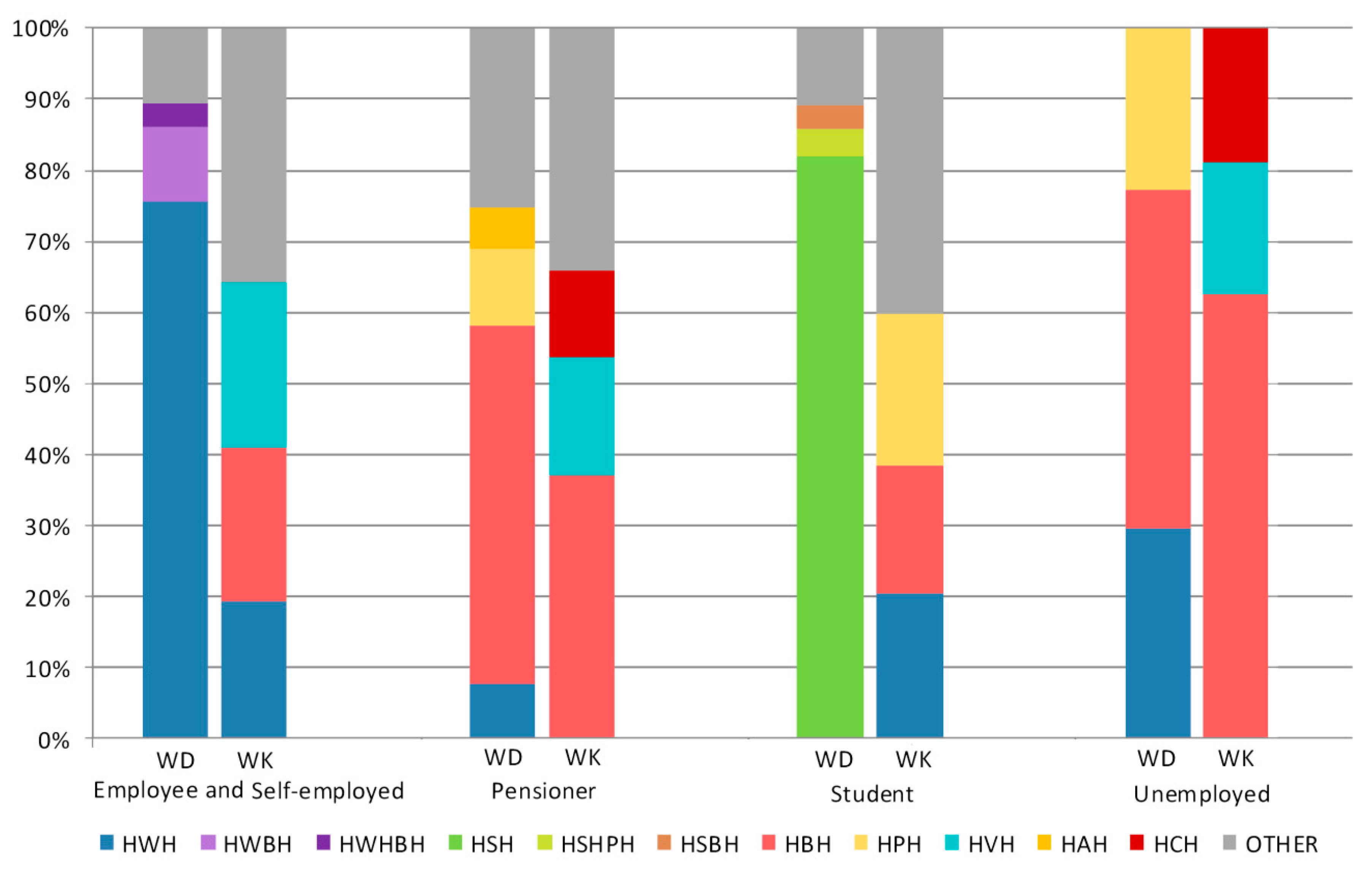
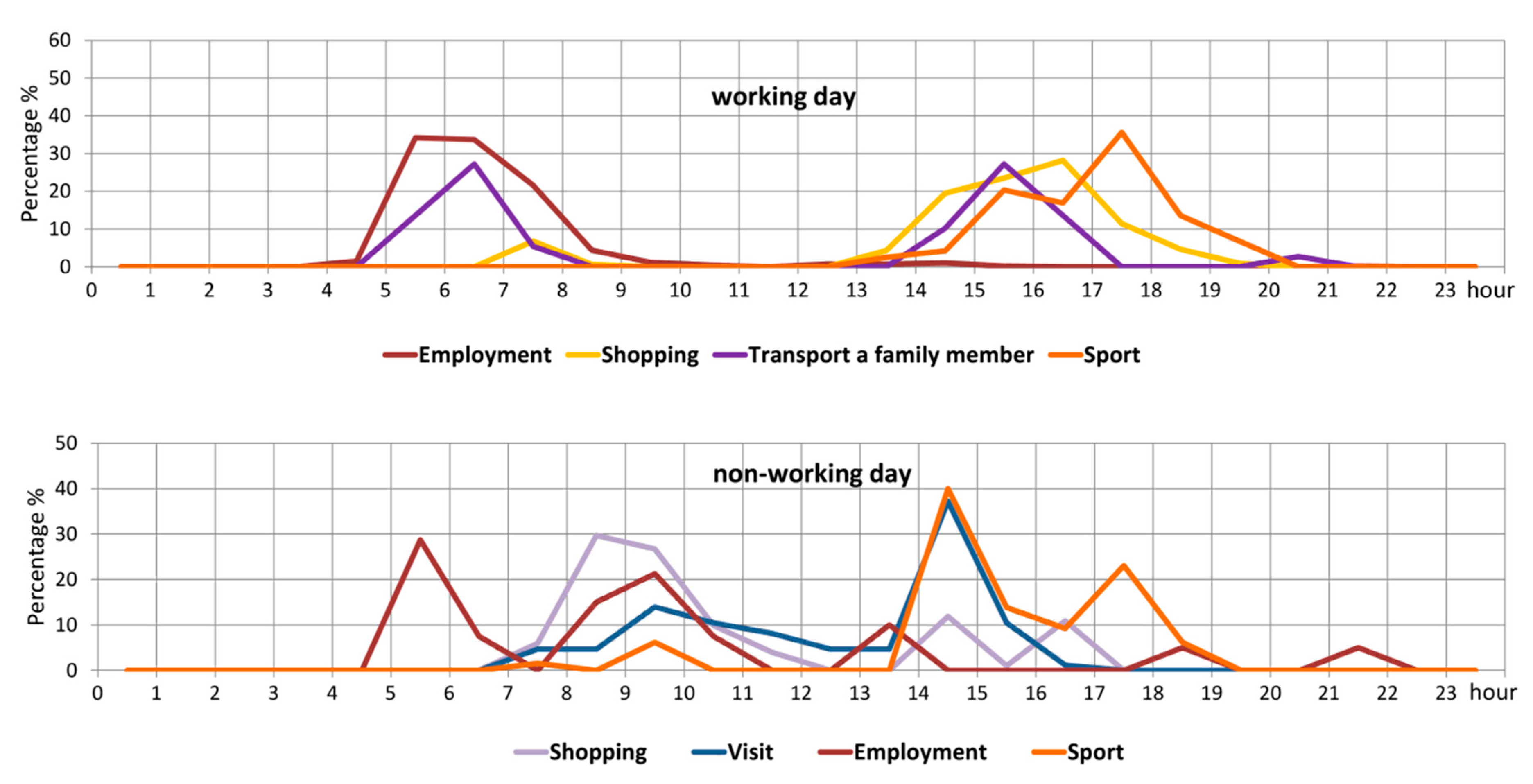
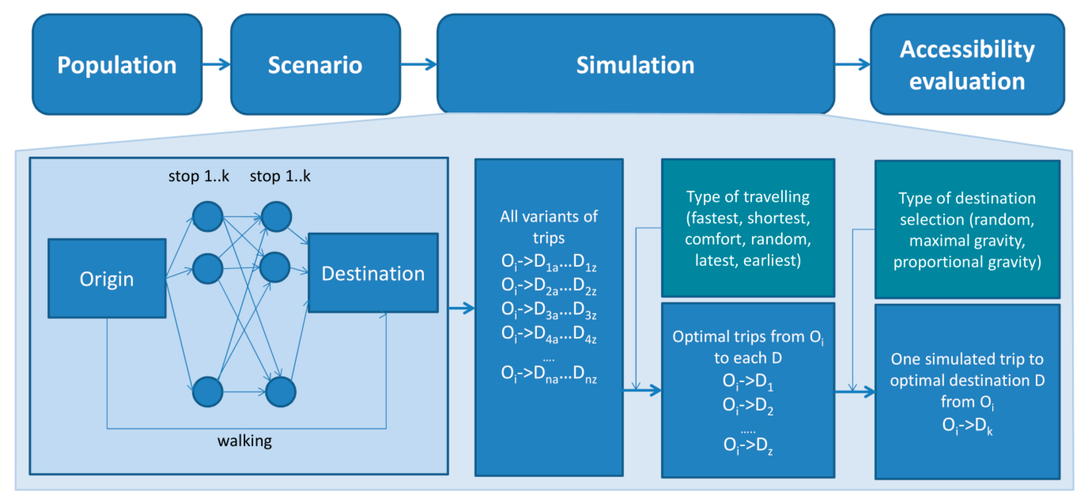
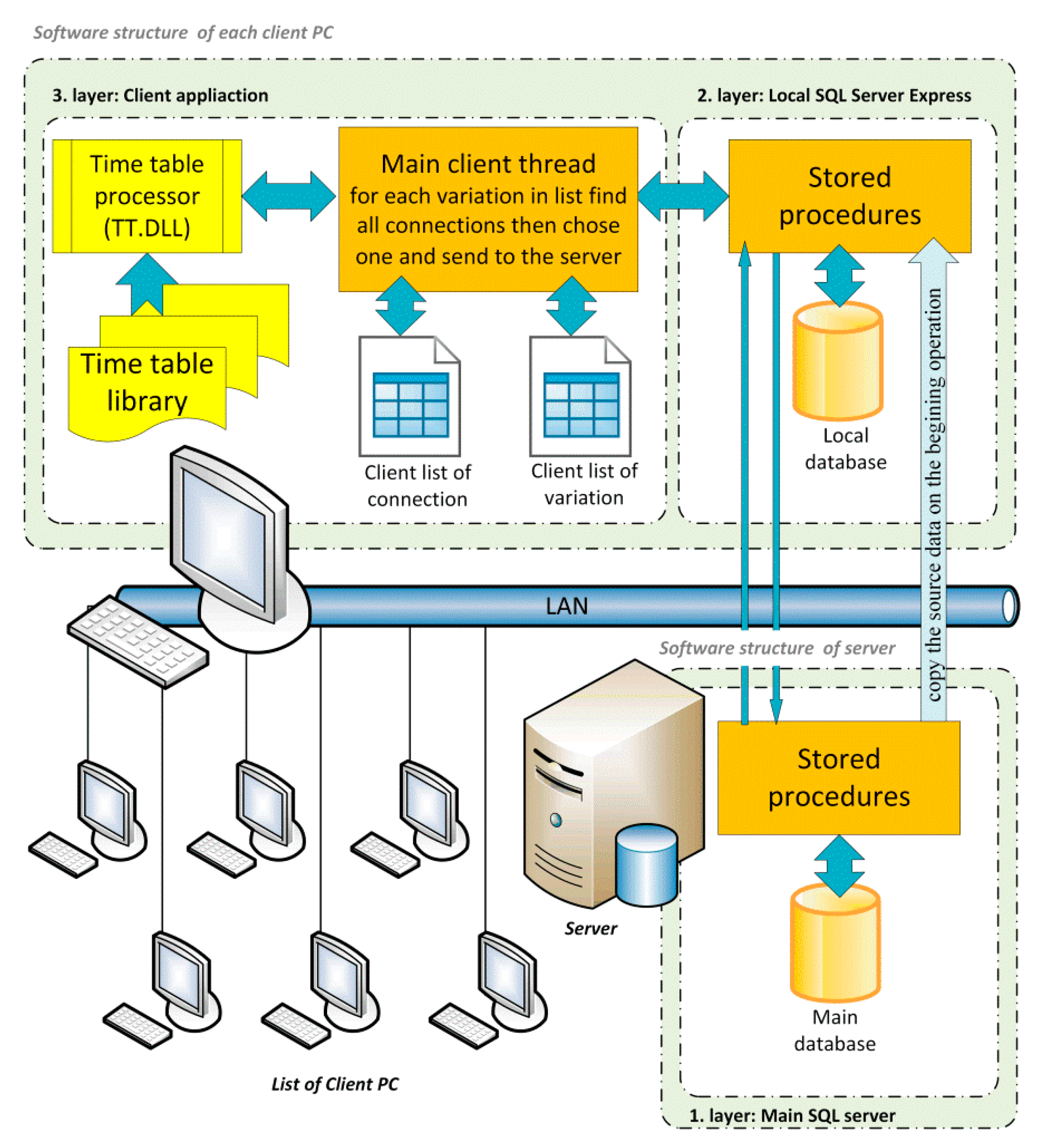
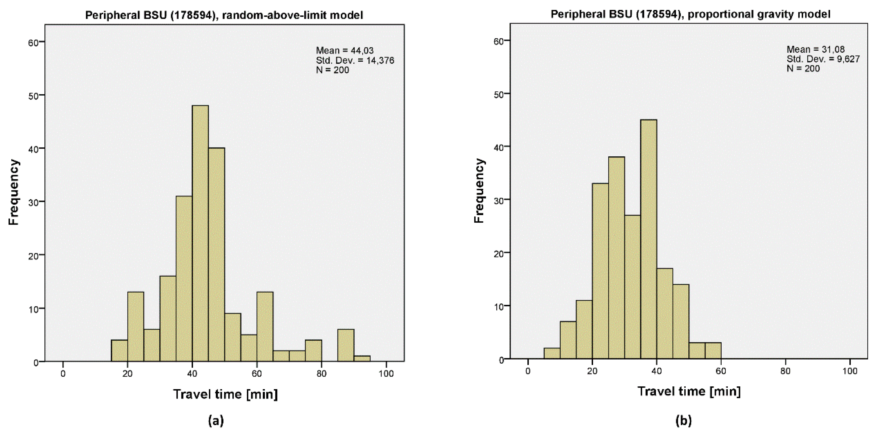
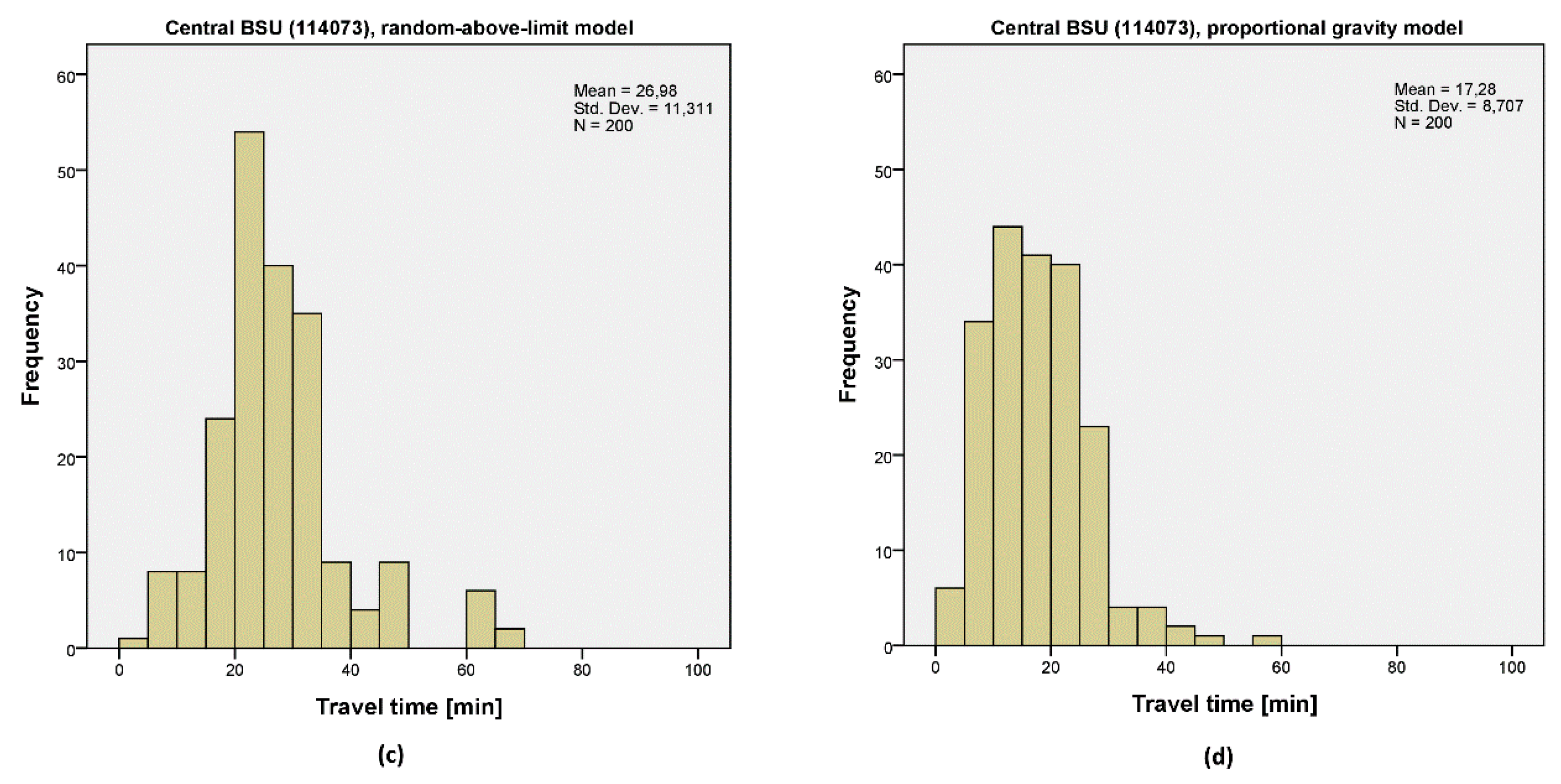
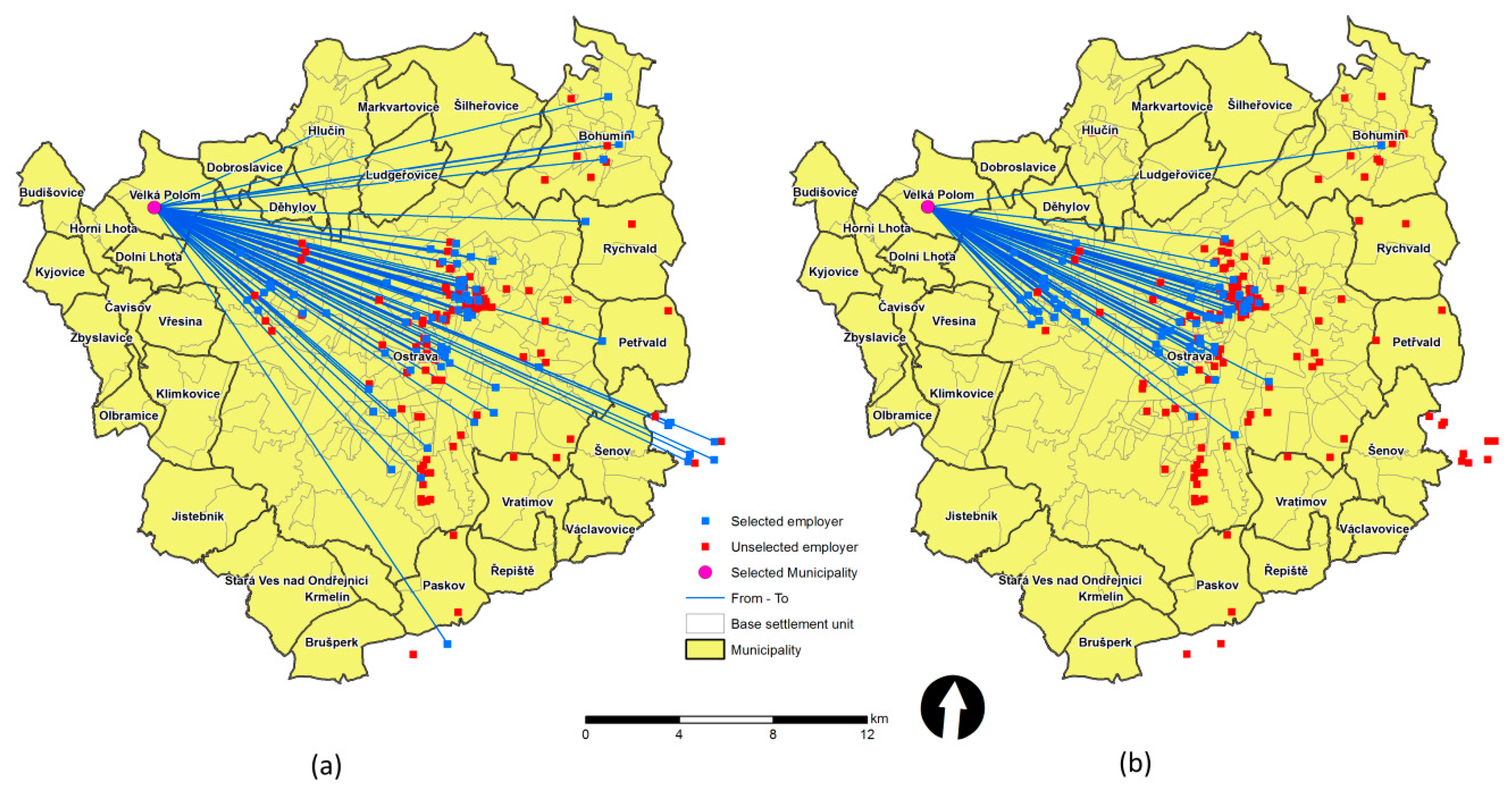
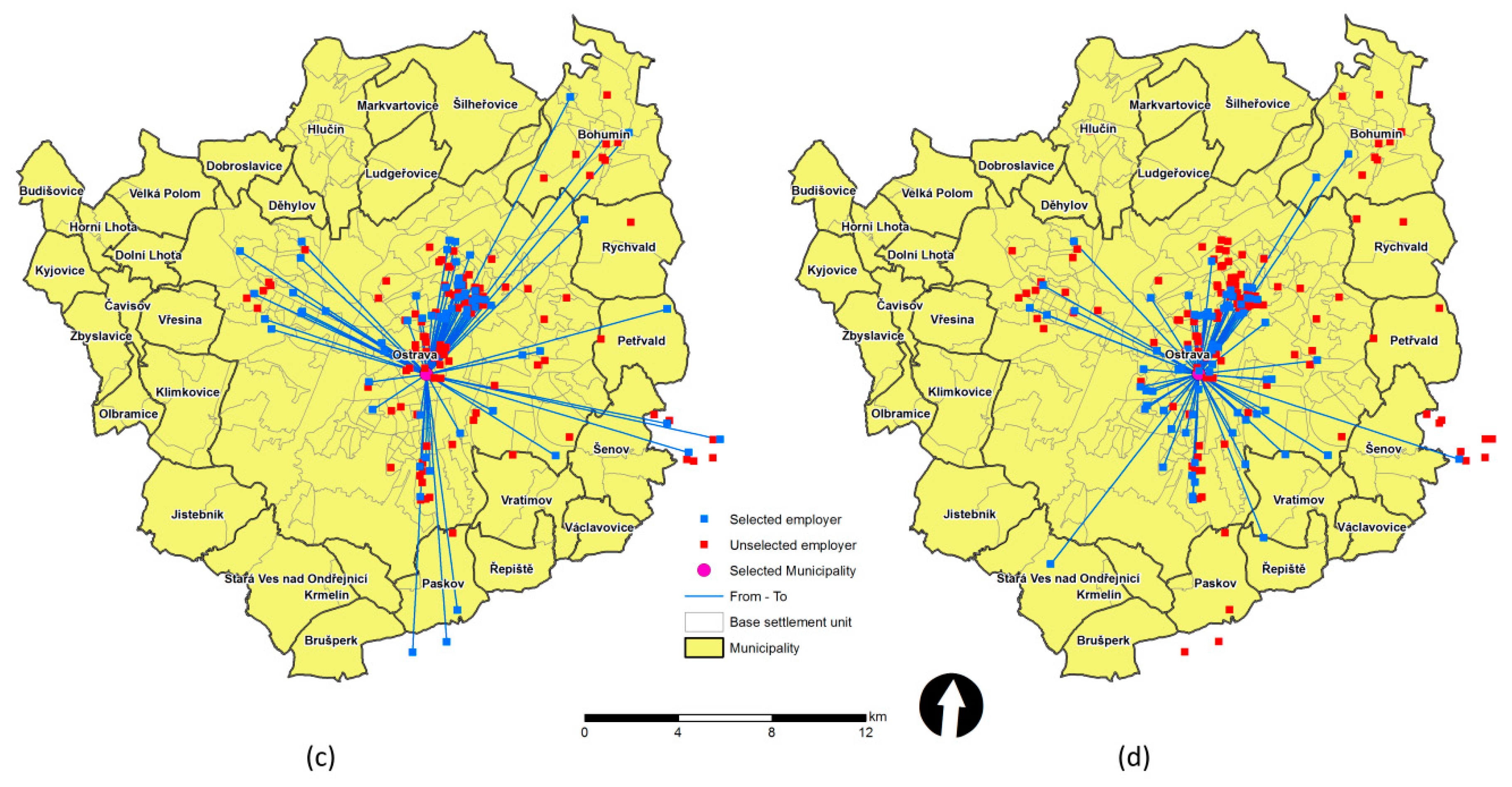
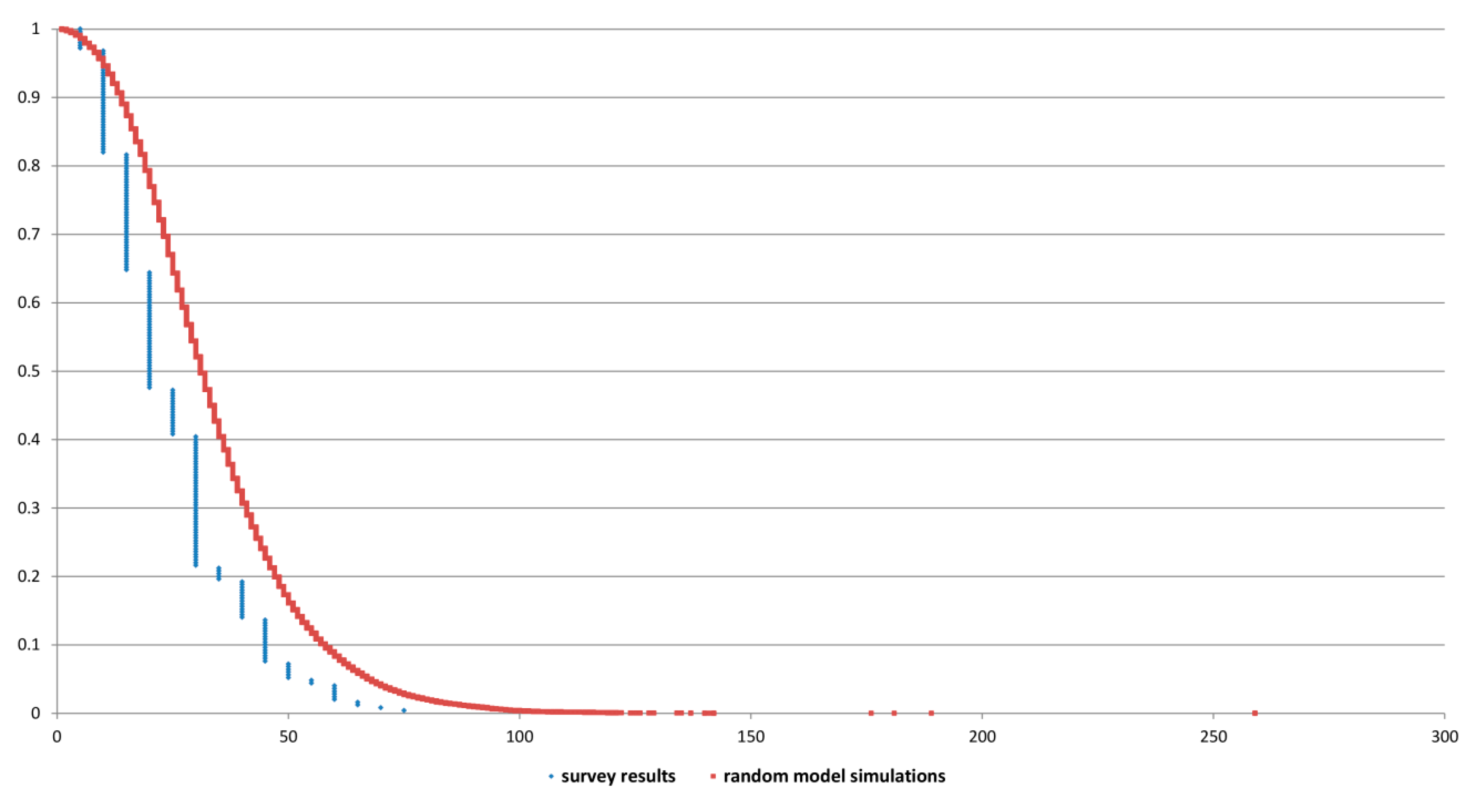
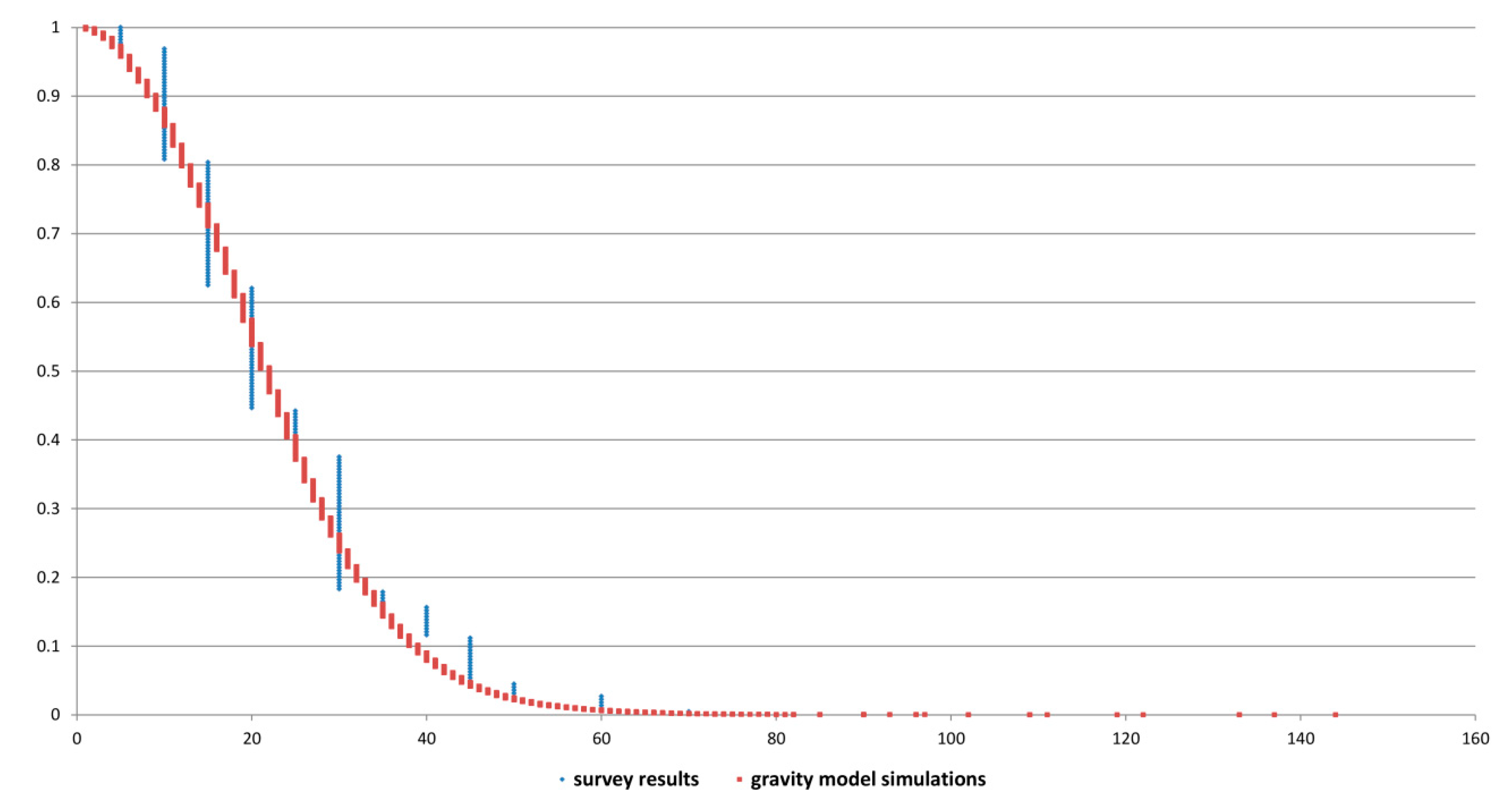
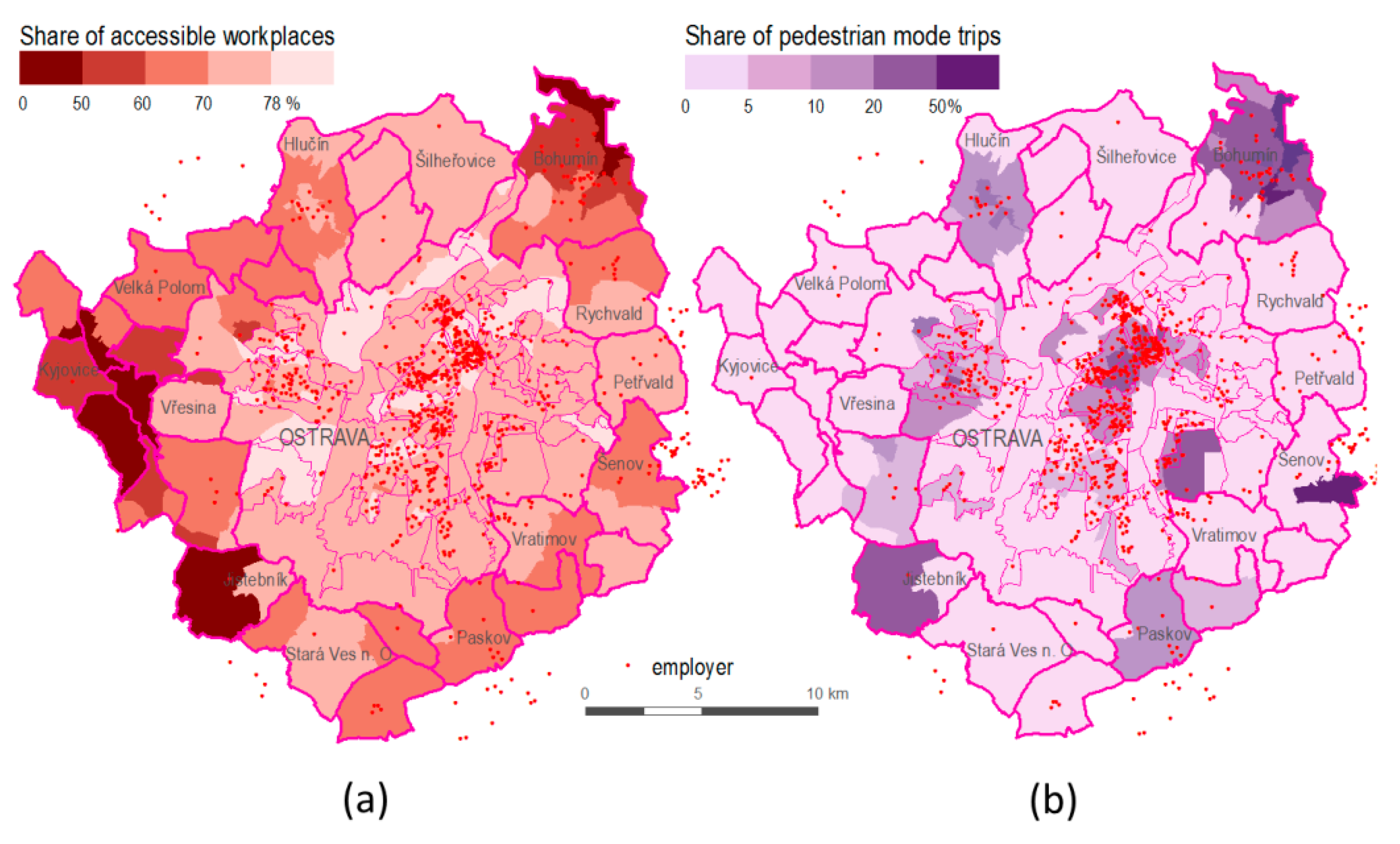
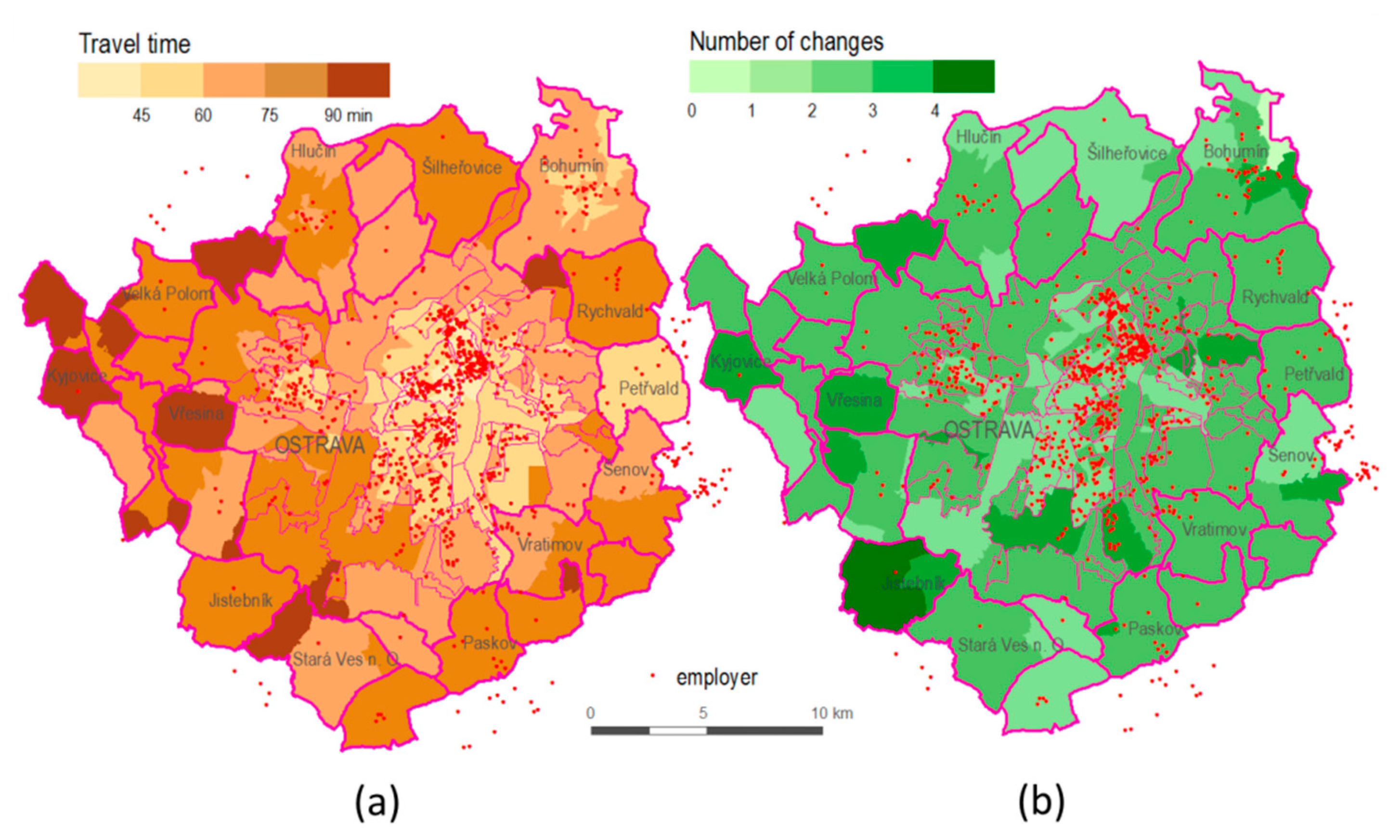
Table 1.
Results for the independence test between the survey and proportional gravity simulation results.
Table 1.
Results for the independence test between the survey and proportional gravity simulation results.
| Test | Kruskal–Wallis Test | Median Test | Jonckheere–Terpstra Test | Mann–Whitney Test | T-Test |
|---|---|---|---|---|---|
| Criterion name | Kruskal–Wallis H | Chi-Square | Std. J–T Statistic | z-score | t-value |
| Criterion value | 1.177 | 0.082 | −0.085 | −1.085 | 1.057 |
| Asymp. Sig. | 0.278 | 0.774 | 0.278 | 0.278 | 0.292 |
© 2019 by the authors. Licensee MDPI, Basel, Switzerland. This article is an open access article distributed under the terms and conditions of the Creative Commons Attribution (CC BY) license (http://creativecommons.org/licenses/by/4.0/).
Share and Cite
MDPI and ACS Style
Horak, J.; Tesla, J.; Fojtik, D.; Vozenilek, V. Modelling Public Transport Accessibility with Monte Carlo Stochastic Simulations: A Case Study of Ostrava. Sustainability 2019, 11, 7098. https://0-doi-org.brum.beds.ac.uk/10.3390/su11247098
AMA Style
Horak J, Tesla J, Fojtik D, Vozenilek V. Modelling Public Transport Accessibility with Monte Carlo Stochastic Simulations: A Case Study of Ostrava. Sustainability. 2019; 11(24):7098. https://0-doi-org.brum.beds.ac.uk/10.3390/su11247098
Chicago/Turabian StyleHorak, Jiri, Jan Tesla, David Fojtik, and Vit Vozenilek. 2019. "Modelling Public Transport Accessibility with Monte Carlo Stochastic Simulations: A Case Study of Ostrava" Sustainability 11, no. 24: 7098. https://0-doi-org.brum.beds.ac.uk/10.3390/su11247098
Note that from the first issue of 2016, this journal uses article numbers instead of page numbers. See further details here.