Sustainable Policy Evaluation of Vehicle Exhaust Control—Empirical Data from China’s Air Pollution Control


1
School of Economics, Sichuan University, Chengdu 610065, China
2
Collaborative Innovation Center for Security and Development of Western Frontier China, Sichuan University, Chengdu 610065, China
*
Author to whom correspondence should be addressed.
Sustainability 2020, 12(1), 125; https://0-doi-org.brum.beds.ac.uk/10.3390/su12010125
Submission received: 26 November 2019
/
Revised: 17 December 2019
/
Accepted: 20 December 2019
/
Published: 22 December 2019
(This article belongs to the Special Issue Environmental Behaviour and Collective Decision Making)
Abstract
:With the increase of car ownership, mobile pollution has become an important source of air pollution, which makes it more difficult for China to control air pollution. In order to control mobile pollution from automobile exhaust, China has taken a series of comprehensive measures. The paper studies the emission reduction effect from the perspective of flow pollution and stock pollution. First of all, the paper uses the actual emission data of motor vehicles to study the emission reduction effect by gasoline and diesel vehicles. The results show that: (1) Fuel price, fuel tax (except diesel), and emission and gasoline standards have an emission reduction effect on gasoline vehicle exhaust control, while the restriction has no effect. (2) In gasoline cars, the emission reduction effect in the Middle East is more significant than in the West, and the effect in the West is better than that in the Middle East. (3) As for diesel vehicles, the effect of policy in the West is superior to the East. Further, the east is better than in the middle. Secondly, based on the actual emission data of Chinese motor vehicles, the paper simulates the change value of stock pollution from automobile exhaust under different policies, and concludes that the economic effect of policy depends on the ecological absorption rate and discount rate. When the net discount value NPV is positive, the government should do its best to interfere with the emission of automobile exhaust. When the net discount value NPV is negative, the government doesn’t have to interfere with the emission of automobile exhaust.
1. Introduction
Environmental issues are a substantial concern among scientists, and the atmospheric environment is particularly. As the world’s second largest economic community, China has achieved great improvement in economic development. Meanwhile, serious haze has occurred in China frequently, especially in areas where the economy grows fast. In 2014, only three cities (Hai Kou, Lhasa and Zhou Shan) of 74 pilot cities in China, the cities that implemented new air standards, completely conformed to the new standard and reached secondary air quality standards. However, air pollution was relatively serious in the Beijing–Tianjin–Hebei region, Yangtze River delta region, and the Pearl River delta region, the main features of which were compound pollution of soot and motor vehicle exhaust. The carbon monoxide (CO), nitrogen oxides (NOX) and particulate matter (PM) in the most cities has already exceeded new air standards badly. There is no doubt that, in China, vehicle exhaust has replaced waste gas produced by the industrial burning of coal as the main source of pollutants in large and medium-sized cities. In 2017, vehicle emissions of NOX and PM exceeded 90% of the total NOX and PM, while HC and CO exceeded 80% of the total HC and CO. In addition, HC, NOX, and other pollutants may also produce harmful secondary pollution-photochemical smog-under the action of sunlight (ultraviolet ray). These pollutants are harmful to human health and reduce the degree of visibility, harm crops, and damage vegetation. Severe traffic pollution is associated with multiple serious health problems, including myocardial infarction [1], stroke [2], asthma [3], and preterm birth [4,5]. Vehicular fossil fuel combustion also makes a great contribution to global warming [6]. Although the atmospheric environment has a certain self-purification capacity, it will exceed the self-purification capacity if we release too much exhaust gas into the atmospheric environment, which will lead to series of atmospheric environmental problems. Depending on local dispersion, populations and values, economists have estimated that the damage to health caused by the motor vehicles exhaust ranges from $0.60 to $1.60 per gallon [7]. These damages cause relatively small losses in the short term but can cause great losses as pollution accumulates. How to control automobile exhaust in a timely manner and achieve stable economic development becomes a challenge for the Chinese government. In order to control automobile exhaust pollution, China has adopted a series of control measures including a fuel tax (1994), vehicle and vessel tax (2007), emissions standards (2000), as well as fuel standards (2001) and restrictions (Seven cities in China have restricted their license plates, and more than 40 cities have issued or temporarily implemented odd-and-even license plate rule or tail restrictions.). Based on those measures, this paper studies these comprehensive policies of automobile exhaust from the perspective of flow pollution and stock pollution. With respect to these policies, we are interested in two research questions. The first is to answer whether these policies play a role in controlling automobile exhaust emissions. How much does each policy contribute? Second, if these policies are effective, is there a positive economic benefit from exhaust emissions reduction?
The rest of the paper is organized as follows. Section 2 reviews the literature. Section 3 presents the empirical facts and the optimal control mechanism for vehicle exhaust. Section 4 introduces the study’s data, variables, and model. Section 5 reports the results of the main tests and offers analysis. Section 6 further studies the economic effect of emission reduction. Finally, Section 7 is a summary.
2. Literature Review
Raising fuel costs represents a feasible way to further control air pollution and promote energy conservation and emission reduction. However, there is no consistent conclusion about the actual impact of fuel prices (taxes) from the perspective of demand elasticity. Higher gasoline prices would encourage people to drive fewer miles and to purchase cars that are more fuel-efficient [5]. However, studies of gasoline demand suggest that raising prices would have only a small impact on driving behavior. Archibald and Gillingham estimate an overall short-run price elasticity (percentage change in miles per percentage change in price) of −0.43 using household data from the 1972 to 1973 Consumer Expenditure Survey [8]. Walls et al. used the 1990 National Transportation Survey to estimate a short-run price elasticity of −0.51 [9]. Drollas estimates a price elasticity of −0.35 over the short run and −0.73 over the long run [10]. Dahl and Sterner (1991 a,b) survey the gasoline demand literature and find mean price elasticity for panel data to be −0.26 over the short run and −0.86 over the long run [11,12]. Johansson and Schipper find similar long-run price elasticities of −0.87 [13]. Above mentioned studies of price elasticity suggest that the short-run price elasticity of fuel is less elastic and long-run price elasticity is more elastic [4], which means that raising prices has only a small impact on air pollution in the short term but a large impact in the long term. Sipes and Mendelsohn studied the impact of gasoline taxes on air pollution in the United States and found that gasoline tax only slightly decreased gasoline consumption, which had little effect on air pollution [14]. Barnett and Knibbs studied how raising diesel prices significantly reduced the concentration of CO and NOX, while raising gasoline prices had no impact on air pollution [5]. Peng and Ruo analyzed different types of vehicles and believed that raising prices could not change the air quality of the overall region. The reason for this is that raising prices had not reduced the miles driven in private cars, buses, and motorcycles, but only reduced the miles of non-private cars and taxis [15]. Some scholars studied the relationship between fuel tax and environmental problems from the general equilibrium. They thought that levying an appropriate fuel tax can improve social welfare, but it will also have some negative effects [16,17].
Reducing the use of motor vehicles to control air pollution is another quick and feasible method, however the effect of restrictions to control air pollution is very limited. Although there have been three decades of practice experience since 1986, when a restrictions policy was first introduced in Santiago, Chile, the literature of quantitative evaluation of restriction was rare [18]. Of the few studies, the evaluation of the one-day weekly restriction policy (Hoy No Circula (HNC) in Mexico City had the most impact. Evidence from Mexico City has shown that wealthy people were able to buy second cars with a different license plate to circumvent the ban, and, therefore, total car use in Mexico City had in fact increased [19]. These additional cars were typically older and generate more pollution, which in turn made the air pollution even worse [20]. Across pollutants and specifications, there was no evidence that restrictions improved air quality [21]. Some argued that instead of achieving the policy goals for a reduction of congestion and air pollution, the regulation was in fact inefficient and unfair [20]. Similar driving bans were introduced in São Paulo, Bogota, and Santiago thereafter. In spite of its popular adoption, the regulation remained controversial. Lin et al. found that São Paulo and Bogotá‘s traffic restriction policies were effective only in the short term, but not conducive to the improvement of air quality in general [22]. One exception was Athens, which has imposed permanent odd–even driving restrictions in the center of the city (“ring”) since June 1982. These measure have been criticized in the sense that while they reduced traffic and pollution in the ring, they also resulted in considerable traffic and pollution problems at the perimeter of the ring [23]. While there were great concerns at home and abroad about the environmental effects of the odd-even driving restriction during the Beijing Olympics and most of which supported the significant positive effect of the policy [22,24,25,26], much less attention has been paid to the post-Olympics 20% restriction scheme. Further, a 20% driving restriction could effectively reduce ambient PM10 levels. However, this positive effect rapidly faded away within a year due to the long-term behavioral responses of residents [18,25,26]. Qi et al. evaluated China’s restriction policy and found that the restrictions are effective for the short-term control of nitrogen dioxide, PM2.5, and sulfur dioxide emissions, but ineffective for the long-term control of this pollution [18].
Most of the research about the effect of vehicle emission standards that improve air quality focuses on environmental science. Rhys-Tyler et al. used remote sensing technology to detect instantaneous exhaust emissions of light vehicles [27]. The results showed that nitrogen and oxygen (NOX) emissions could be reduced by 30% under Euro V emission standards. Wu et al. analyzed the implementation of new emission standards and other control measures to find they reduced the emission rate of vehicle pollutants in Beijing [24]. Ren and Wang thought that the emission standards I of motor vehicles had reduced the emission of air pollutants by 57%, which controlled the total emission of motor vehicles effectively in china [28].
There is a relatively large body of literature about the emission reduction policy of automobile exhaust, but their studies have the following shortcomings: First of all, these literatures mostly adopt air pollution monitor value of the whole region as the substitute variable of automobile exhaust [21,26,27,28]. The monitor value of air pollution in the whole region is stock pollution, while emissions from vehicles are flow pollution. Substituting stock pollution for flow pollution could not truly reflect the role of policy. Secondly, most of them only consider the role of a single emission reduction policy and ignore the joint role of different policies, so the evaluation of policies is not accurate enough.
Based on the deficiencies of existing literature, the novelty of our approach might be manifest in several aspects:
- We distinguish the flow and stock pollution of vehicles and further study the effect of emission reduction using the actual emission data of 31 provinces and municipalities in China.
- We analyze the effect of emission reduction of mixed policy-fuel price, fuel tax, emission standards, fuel standards, and restrictions, to improve these mixed policies and to further provide feasibility advice for the control of automobile exhaust.
- We estimate the economic effects of emission reduction policies using actual data of automobile exhaust and calculate the stock pollution in the different dissipation rates.
3. Empirical Fact and Optimal Control Mechanism of Automobile Exhaust
3.1. Empirical Fact
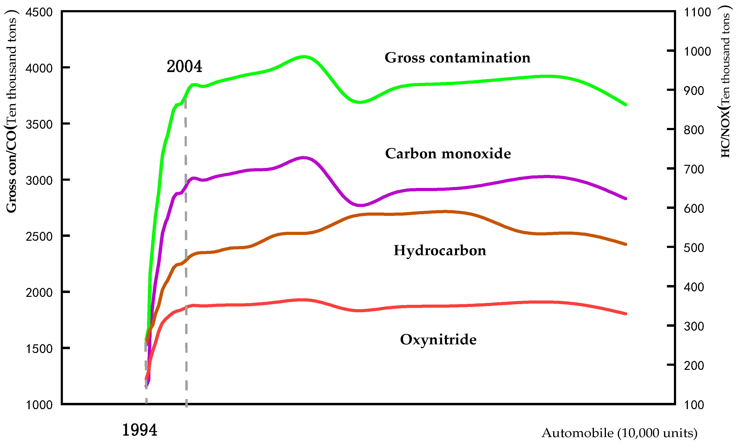
Figure 1 shows the relationship between the number of cars and the degree of pollution. As can be seen from Figure 1, the number of cars increased from about 9 million in 1994 to more than 200 million in 2017, which increased by nearly 20 times. However, the pollution emitted by cars increased from 15 million tons to 40 million tons, and then decreased to 35 million tons, which increased by less than 3 times. This shows that the rate of increase automobile exhaust is far less than the rate of increase automobile. From 1994 to 2004, the amount of automobile exhaust emissions increased sharply, then increased slowly and began to decrease in 2010. During this period, China implemented a series of policies to control automobile exhaust. It can be seen from the empirical facts that these policies play an important role in reducing automobile exhaust.
3.2. Optimal Control Mechanism of Vehicle Exhaust
The model of optimal control theory given below is mainly learnt from Alpha C. Chiang [29]. In the process of fuel consumption, energy will be consumed and a large amount of pollution will be generated. refers to the using amount of fuel energy. refers to the stock pollution generated by vehicle exhaust, and refers to the flow pollution. Fuel oil is referred to as energy in the following analysis. Automobile exhaust is called pollution for short. Assume that there are motor vehicles and automobile exhaust are directly proportional to energy use. Now set () as the scaling factor, which is expressed as:
At the same time, the pollution dissipates and decreases at the rate of , .
The stock of pollution at time is,
The use of energy raises the social utility, while the accumulated pollution also raises the negative social utility. The social utility function depends on the energy consumption and accumulated pollution. The function of energy consumption and accumulation pollution is as below respectively:
The utility function of the society is:
and it has the following derivative:
Now the environmental protection department plans to optimize the utility in a given period , as follows:
Constructing the Hamilton function:
maximize the first order condition:
The cross-sectional condition is:
By , the increased social utility of energy transport and reduced social utility caused by accumulated pollution depend on the shadow price of accumulated pollution (), the scaling factor of energy and pollution (), and the dissipation rate (). In the formula, the first item, , measures the marginal positive utility from energy consumption. The second item in the above, , measures the marginal negative utility of accumulated pollution from time 0 to .
When the dissipation rate meets the following conditions, , the initial emission is completely dissipated. At this time, the increased social utility of energy transportation is exactly equal to the reduced social utility of accumulated pollution, namely .
Since the equation above is independent of the time variable , the solution of optimal energy use is constant:
This means that the use of any unit of energy will not increase or decrease the utility of the whole society, so the government does not need to intervene in the emission of automobile exhaust at the beginning. When the dissipation meets the following conditions, , the sum of the increased social utility from energy transportation and the reduced social utility from accumulated pollution is negative, namely, . This indicates that the pollution generated by any unit of energy use will be accumulated and the negative social utility taken by accumulated pollution is bigger than the positive social utility generated by energy use, which finally reduces the whole social utility. Therefore, the government needs to intervene in the emission of automobile exhaust so that the speed of emission is equal to the speed of dissipation of pollution, that is,
Ultimately, the total social utility is zero, .
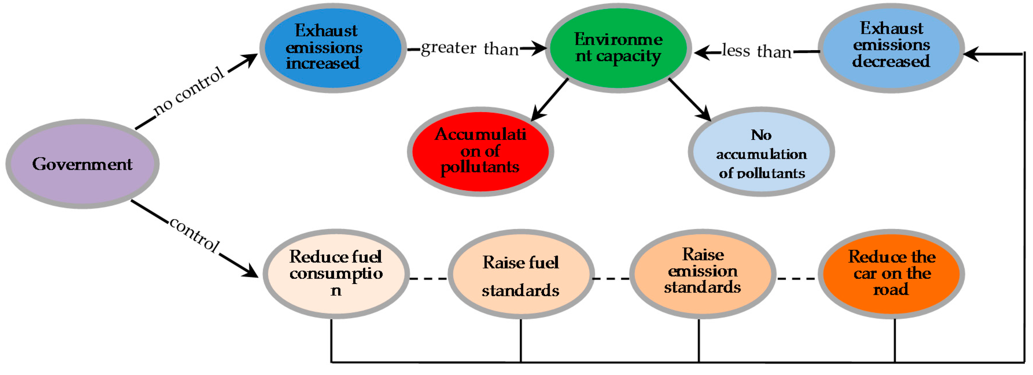
From the above derivation, it can be seen that, when the flow pollution of automobile exhaust is greater than the dissipated pollution, the environmental protection department needs to intervene in the emission of automobile exhaust at the beginning and vice versa. Hence, the environmental protection department can use such a policy to raise the fuel price to reduce energy consumption or restrict the number of miles driven to control automobile exhaust. It can also improve the engine standards and fuel standards to reduce the emission of unit exhaust through technological progress to control automobile exhaust. The logical derivation is shown in Figure 2. Based on that, the paper constructs an econometric model to test the emission reduction effect of several control policies and simulates economic effect of emission reduction.
4. Model and Data
4.1. Model Construction
In order to analyze the emission reduction effect of automobiles, we select five main control policies, namely net fuel price, fuel tax, emission standards, fuel standards, and traffic restriction. Based on the theoretical model, the paper constructs the following measurement model by referring to the models of J.V. Henders [30], Penghui X. [15], Hongyou L. et al. [31], Kunxin S. [32], Eskeland [20], and Jing C. [26]:
In Equation (14), the explanatory variable is , which represents the vehicle exhaust emissions of the province and the pollutants are carbon monoxide, hydrocarbons, and nitrogen oxide dyes. The core explanatory variables () are the net fuel price, fuel tax, emission standards, fuel standards, and driving restriction, respectively, where represents the number of cities in province that are restricted (Restricted city is 1, unrestricted city is 0). is the set of control variables. Firstly, the number of vehicles is added to the model to control the influence of vehicle, which will increase the emission of vehicle exhaust. The second control variable is fuel consumption, which controls the impact of the actual change of fuel consumption on exhaust emissions. The third is GDP per capita, controlling the influence of economic development. Fourthly, vehicle and vessel tax are added to control the influence of vehicle and vessel tax on automobile exhaust emission. Where , , , and are the coefficients of the main explanatory variables, is the coefficient of the control variables, is the fixed effect of provinces and municipalities (only gasoline), and is the disturbance term.
In order to make the regression results reliable, we select three major components of exhaust emissions as explanatory variables: Carbon monoxide (CO), hydrocarbons (HC) and nitrogen oxides (NOX). The reason for choosing these variables is based on the classification of data in China’s motor vehicle management environment annual report. To keep the data stable, the logarithm of the explained variable is taken. Core explanatory variables are:
- Net fuel price and fuel tax. Because the actual fuel price includes fuel taxes, we divide it into net fuel prices and fuel taxes.
- Emission standards. The emission standards for motor vehicles are based on the emission limits and measurement methods for light vehicles. In the index, the substitution variable of the emission standards is the emission standards limit in 2000 minus the emission standards limit in practice in that year ().
- Fuel standards. The computing method of fuel standards is the same as emission standards. ().
- Restriction. Virtual variables are used instead (Restricted city is 1, unrestricted city is 0).
In order to keep the data stable, the core explanatory variables are logarithmically processed.
4.2. Data
The samples of this paper are taken from 31 provinces (municipalities) in China, including 22 provinces, five autonomous regions, and four municipalities directly under the central government. Because the political systems in Hong Kong, Macao, and Taiwan are different from that in mainland, the samples in this paper do not cover samples in Hong Kong, Macao, and Taiwan. Table 1 presents the descriptive statistics of the main variables. We select the source of the main data from China’s motor vehicle environmental management reports, ministry of finance of China, and information network of the development research center of the state council (DRCNET). The data of urban restriction are obtained from the traffic information website of the restricted city. The sample covers the year from 2010 to 2017, which is divided into two samples according to fuel type, namely gasoline vehicle and diesel vehicle. A total 248 samples are included.
5. Estimation and Results
5.1. Baseline Regression Results
Based on the above analysis, this paper studies the emission reduction effect of control policies of automobile exhaust and the specific results are shown in Table 2. In Table 2, the explanatory variable in columns 1 and 2 is carbon monoxide, the explanatory variable in columns 3 and 4 are hydrocarbons, and nitrogen oxide is in column 5 and 6. Each explanatory variable is divided into gasoline and diesel vehicles. After statistical testing, the regression result related to gasoline vehicle is the estimated result under fixed effect, while the diesel vehicle is the estimated result under mixed regression.
According to Table 2, the net fuel price, fuel tax, emission standards and fuel standards of gasoline vehicles are significant under the level of 5%. The coefficient of which is negative, while the restriction is not significant. The net fuel price, emission standards, and fuel standards of diesel vehicles are significant at the level of 5%, the coefficient of which is negative, while the coefficients of fuel tax and restriction are not significant. We draw the conclusion that control policies, namely net gasoline price, gasoline fuel tax, emission standards, and gasoline fuel standards, have a good emission reduction effect on gasoline cars. As for diesel cars, there are three control policies having a good emission reduction effect, which includes net diesel price, diesel vehicle emission standards, and diesel fuel standards. The effect of diesel fuel tax is not significant. The possible reason for this is that the diesel fuel tax is lower than gasoline, and its tax has less of an impact on diesel consumption. Secondly, in reality, the annual diesel consumption is increasing year by year. However, the annual gasoline consumption is decreasing. The effect of restriction on gasoline and diesel vehicles is not ideal. The internal reasons may be as follows: Firstly, restriction has obviously reduced the use of cars in short terms, but it will be weakened in the long term as the number of cars increases [19]. Secondly, the effect of partial city restrictions is limited to the emission reduction of motor vehicle exhaust in the whole province.
In the model, it can be seen that the marginal emission reduction contribution of five control policies in gasoline vehicles is in order: Fuel standards, fuel tax, fuel prices, and emission standards and restriction. This shows that fuel standards, fuel taxes, fuel prices, and emission standards can be the government’s preferred tools controlling gasoline vehicle exhaust. In diesel vehicles, the marginal emission reduction contributions are in the following order: Emissions standards, fuel price, fuel standards, fuel tax and restriction, showing that fuel prices, emissions standards, and fuel standard can be used as the preferred tools to control the diesel automobile exhaust.
5.2. Endogenous Discussion
In the above model, there may be an endogenous relationship between net fuel price and fuel tax and automobile exhaust, which can lead to biased results. This paper adopts instrumental variable method to deal with endogenous problems. In terms of panel data model, if there is autocorrelation and heteroscedasticity, the estimation results of two-stage least square method (2SLS) may be biased and generalized method of moments (GMM) is more effective than 2SLS. In the selection of instrumental variables, individual income tax, commodity consumption tax and housing expenditure are used as the instrumental variables of net fuel price and fuel tax. The reason for choosing these substitution variables as instrumental variables are that the increase of personal income tax, commodity consumption tax and housing expenditure will crowd out self-driving travel consumption and the household income will not be changed. Therefore, individual income tax, commodity consumption tax and housing expenditure are taken as instrumental variables to solve the endogenous problem. Specific results are shown in Table 3.
5.3. Robustness Test
Due to the choice of index, net fuel price, fuel tax, emission standards, and fuel standards are subjective. The results may be different. Therefore, the above variables are changed into fuel price, the proportion of fuel tax in fuel price, and the dummy variable of emission standards and fuel standards for re-estimation and a robustness test. The results are shown in Table 4. According to the robustness test, the estimated results are very similar to the previous.
The fuel price, fuel tax, emission standards and fuel standard of gasoline vehicles are negative at the level of 5%. The coefficient of restriction is not significant under the fixed-effect and the coefficient is positive in instrumental variable-generalized method of moments (IV-GMM) estimation. The fuel price, emission standards, and fuel standards of diesel are negative at the level of 5%, the restriction coefficient is not significant, and the fuel tax coefficient is positive. Further, it explains that gasoline price, gasoline fuel tax, gasoline emission standards and gasoline standards have emission reduction effect on controlling gasoline automobile exhaust, while the restriction has no effect. Diesel price, emission standards and fuel standards have an emission reduction effect on diesel vehicle exhaust, while restriction and diesel fuel tax have no emission reduction effect.
5.4. Heterogeneity Analysis
We divide the types of provinces (municipalities) into eastern, central and western regions to further investigate the heterogeneous effect of control policies. The regression results of carbon monoxide are shown in Table 5 (The regression results of hydrocarbons and nitrogen oxides are similar to carbon monoxide). According to the statistical test, the regression results of the eastern and central regions are estimated result under fixed effects, while the western regions are estimated result under mixed regression.
Among gasoline vehicles, four control policies (gasoline price, gasoline tax, emission standards, and gasoline standard) in the eastern and western regions have a strong regulating effect controlling exhaust of gasoline vehicles. Three control policies (gasoline price, gasoline tax, and gasoline standard) in the central region have a strong regulating effect. Moreover, the regression coefficient in the east is larger than that in the central and western regions, indicating that the effect in the east is more significant than that in the west, and the effect in the west is better than that in the middle region.
In diesel vehicles, the two policies (diesel price and diesel standard) in the eastern region, a policy (diesel standard) in the central region and three policies (diesel price, emission standards and diesel standard) in the western region have a strong regulating effect on controlling the exhaust of diesel vehicle exhaust, which indicates that the effect of control policy in the western region is more significant than that in the eastern region and the result is more significant in the eastern than central region.
At the same time, in order to explain the influence of restriction policies, the provincial (municipal) samples are divided into restricted areas and non-restricted areas and the regression results are shown in Table 6. According to the statistical test, the regression results in restricted areas (except diesel vehicles in hydrocarbon) are the estimated results under fixed effects, while the regression results in the non-restricted areas are the estimated results under mixed regression. In the restricted areas, four kinds of control policies (gasoline price, gasoline tax, emission standards, and gasoline standards) have a strong regulating effect on controlling exhaust generated by gasoline vehicles. For diesel vehicles, the fuel tax effectively controls the emissions of carbon monoxide and hydrocarbons and diesel prices, emission standards and diesel standards can control nitrogen oxide emission. In non-restricted areas, there are four control policies (gasoline price, gasoline tax, emission standards, and gasoline standard) that have a strong effect on controlling gasoline automobile exhaust. Meanwhile, there are three control policies (diesel price, emission standards, and diesel standard) demonstrating a great effect on controlling exhaust of diesel automobile.
6. Further Analysis of Exhaust Control Policies
6.1. Accumulation and Influence of Exhaust under Different Policies
As flow pollution is discharged, stock pollution accumulates, but a portion of the annual stock pollution will dissipate. Therefore, assuming that the stock pollution starts from zero, which means that, there is no stock pollution in 2009, then the stock pollution in 2010 will be:
The stock pollution in 2011 is equal to the pollution that hasn’t dissipated in 2011 plus the stock pollution that hasn’t dissipated in 2010:
Generally speaking, the stock pollution in year is equal to the undissipated pollution in the current year, plus the stock pollution in the previous year:
According to Equation (3) and the actual emission data of automobiles in China, the change value of stock pollution of automobile exhaust under different policies is simulated, and the specific results are shown in Table 7. In Table 7, the third column is the flow pollution of automobile exhaust (), which is the actual emission of automobile. The fourth column is the emission reduction rate of automobile exhaust relative to 2010. The fifth to eighth columns are listed as stock pollution of automobile exhaust. The flow pollution of automobile exhaust reflects the role of emission reduction policy in the current year and the stock pollution of automobile exhaust depends not only on the role of emission reduction policy but also on the ecological absorption rate. When the flow pollution remains unchanged, stock pollution decreases with the increase of ecological absorption rate. As shown in Table 7, when the absorption rate is , the accumulation speed of automobile exhaust is very fast; when the absorption rate is , the accumulation of automobile pollution gradually decreases; when the absorption rate is , the automobile exhaust is completely absorbed.
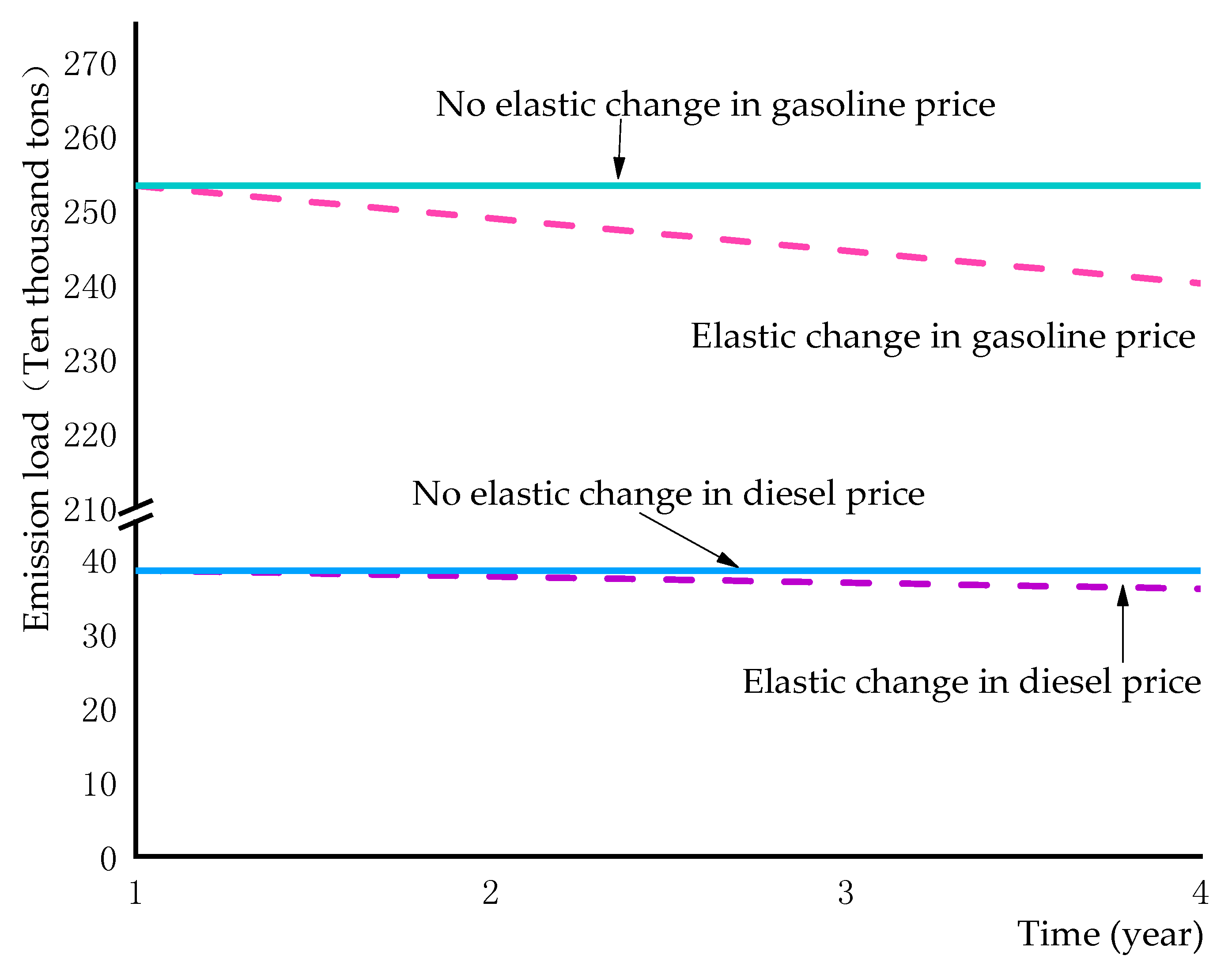
The second row in Table 7 simulate on the changes of flow pollution of vehicle exhaust when fuel price rise by one Yuan in 2010. As seen from the Table 7, emissions reduce from 29.18 million tons in 2011 to 26.31 million tons in 2017, which means that if the fuel price rises by one Yuan, the exhaust may be reduced by about 2.87 million tons in seven years. The contribution of exhaust emission reduction is 13% relative to 2010. The reason for this is that the rise of fuel price and fuel tax affects the demand of fuel and further influences the exhaust emission and the long-term demand elasticity of fuel is much more elastic than the short-term demand elasticity, as shown in Figure 3.
Higher gasoline and diesel prices can reduce the number of miles driven, reducing fuel demand and emissions in the short term. However, the biggest impact of higher fuel prices is to encourage consumers to buy smaller, more fuel-efficient cars. Because car inventories change only slowly, fuel demand falls only slowly with automobile exhaust.
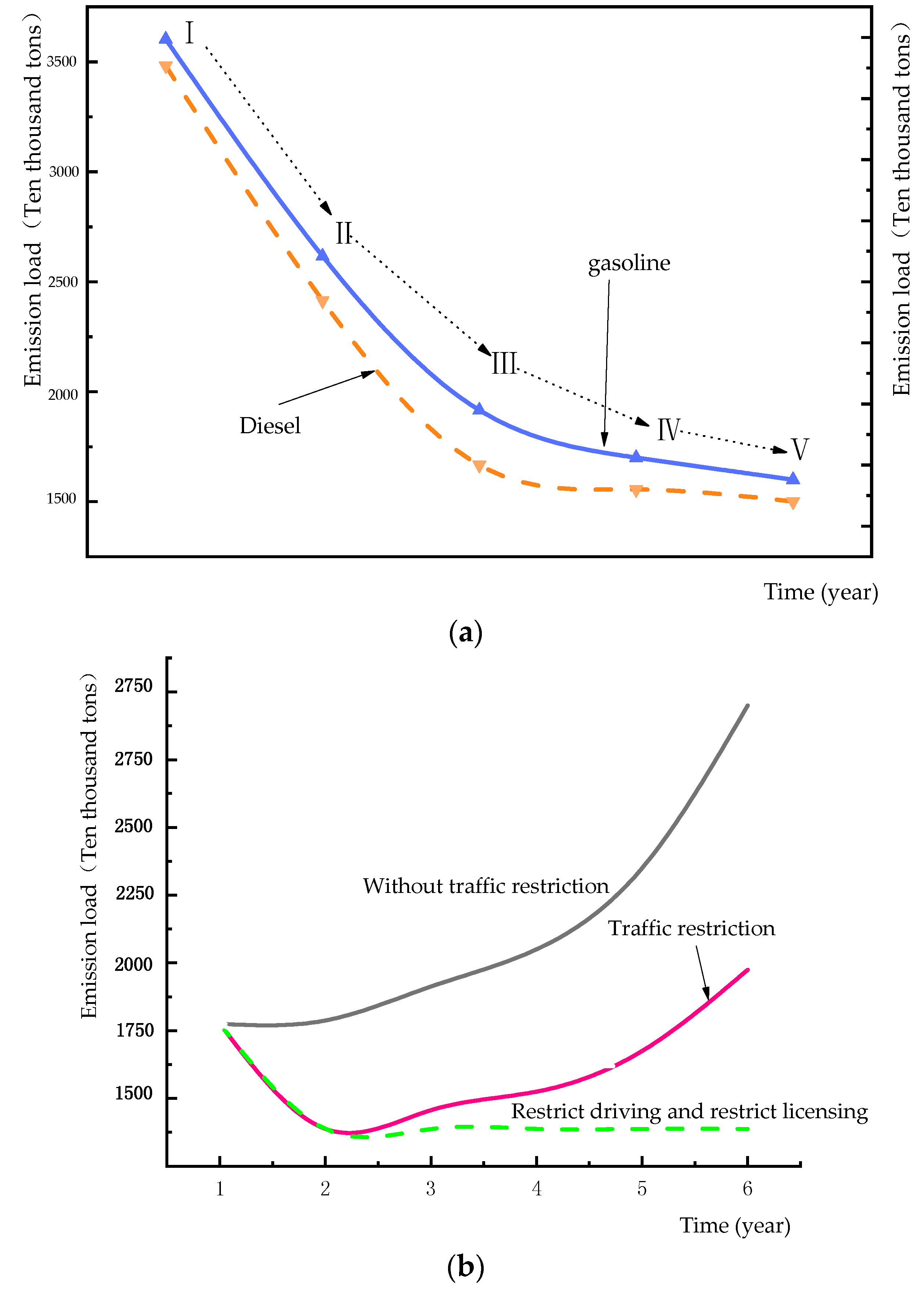
The improvement of emission standards and fuel oil standards will reduce the emission coefficient of pollution, as shown in the third row of Table 7. When the emission standards and fuel standards are enhanced (), the changes of automobile exhaust reduced from 29.14 million tons in 2011 to 25.11 million tons in 2017. The exhaust emission reduction contribution is 17%. The reason for this is that the improvement of emission standards and fuel standards can reduce pollutants from car kilometers per unit, as shown in Figure 4a. With the improvement of the standard, the emission of exhaust will gradually decrease with the other conditions will not be changed.
In the case of other unchanged conditions, restriction in the short term has a good effect on controlling the flow pollution of automobile exhaust, but in the long term its effect will be offset by additional cars. The fourth row in Table 7 simulates that after carrying out the restriction of even–odd automobile exhaust decreases from 40.23 million tons (2010) to 16.25 million tons (2011). Then, it gradually increases to 25.57 million tons in 2017. The fifth row in Table 7 simulates that after carrying out the restriction of even–odd and limiting the number of new license plates, the automobile exhaust decreases from 40.23 million tons in 2010 to 15.07 million tons in 2017. During this period automobile exhaust does not change and the contribution of emission reduction is 50%.
As shown in Figure 4b, odd–even license plate and tail-plate restrictions have good effects on exhaust gas control in the short term, but their effects will be offset with the addition of new vehicles in the long term. However, the implementation of both policies: License plate and restrictions, vehicle exhaust emissions will be controlled within the target range.
6.2. Economic Benefits of Automobile Exhaust Reduction
In order to further measure the net benefits of exhaust reduction policies, this paper estimates the exhaust governance cost and accumulated losses based on the emission reduction cost of waste gas (RMB 218.83 billion) and the cost of environmental loss (degradation) (RMB 219 billion) in the China green GDP accounting research report in 2004 and China environment yearbook, as shown in Table 8.
In Table 8, we use three modes of no reducing emission, reducing emission by 5% and reducing emission by 10% to analyses net benefits of exhaust reduction policies. And represents flow pollution, represents stock pollution at time , the loss refers to the cost of damage caused by the accumulation of automobile exhaust to ecological function, human health, crop yield, etc, the cost represents the cost of reducing emissions, and the net benefit is equal to the loss of no emission reduction minus the accumulated loss of pollution after emission reduction and the cost of emission reduction itself. As can be seen in the ninth and fourteenth row of Table 8, the net benefit of reducing emissions by 5% in 2010 is −100 million Yuan and the net benefit of reducing emissions by 10% is −200 million Yuan, indicating that the cost of emission reduction in that year is higher than that of no emission reduction. It further means that the emission reduction in that year has no economic benefit. The net benefit with greater emission reduction is also smaller. However, the net benefit of reducing emissions increases over time and the net income of emission reduction by 5% is 160 million Yuan (reduced emissions by 10% is 330 million Yuan) in 2017. This shows that cost of emission reduction is far less than the sum environmental loss caused by accumulated pollution, which means that emission reduction in the future will increase profits.
In order to determine whether the emission policy is reasonable, it is necessary to consider the net discount value () of the policy, namely the present value of net income (2010) in Table 8, the calculation formula of is:
In formula (17), is the loss caused by accumulated pollution without emission reduction, is the loss caused by accumulated pollution after emission reduction, is the cost of emission reduction in the current year, and is the discount rate. depends on the discount rate and dissipation rate . The higher the discount rate , the larger the dissipation rate and the smaller the net discount value and vice versa. The results are shown in Table 9.
As shown in Table 9, the net discount value of emission reduction policy depends on the dissipation rate and discount rate. When the discount rate remains unchanged, the smaller the dissipation rate is, the higher the accumulation of pollution will be, and a large economic loss will be generated. Therefore, emission reduction per year will gain more benefits in the future and vice versa. When the dissipation rate doesn’t change, the smaller the discount rate is, the more economical under the initial emission reduction is, otherwise. When dissipation rate is equal to and discount rate is equal to , the net discount values corresponding to emission reduction of 5%, 10%, 20% and 30% respectively are: 6.12, 12.25, 24.49, and 36.74. In the case of dissipation rate is equal to and discount rate is equal to , the net discount values corresponding to emission reductions of 5%, 10%, 20%, and 30% are respectively: −1.41, −2.83, −5.66, and −8.49. This indicates that when the dissipation rate and discount rate are smaller, the emission reduction per year is higher, and the net discount value is larger. When the dissipation rate and discount rate are larger, the annual emission reduction is larger and the net discount value is lower. When the net discount value is positive, the annual emission reduction (5%, 10%, 20%, and 30%) achieves positive economic effects, which means that any emission reduction will generate benefits. Therefore, the government needs to make the greatest efforts to intervene in the emission of automobile exhaust at the beginning of 2010. When the net discount value is negative, it indicates that the annual emission reduction (5%, 10%, 20%, and 30%) gains negative economic effects, which means that any emission reduction will cause loss, so the government does not need to intervene excessively in the emission of automobile exhaust at the beginning (2010).
7. Conclusions
This paper studies the emission reduction effect of diesel vehicles and diesel vehicles in different provinces (municipalities) by using the actual emission data of 31 provinces (municipalities) in China from 2010 to 2017. The basic estimation results are obtained by using fixed effect (diesel) and mixed regression (diesel) and more reasonable estimation results are obtained using the IV-GMM method in dealing with endogenous problems. The results show that: First of all, fuel price, fuel tax (except diesel), emission standards, and fuel standards have an emission reduction effect on controlling vehicle exhaust, while restriction has no effect. Secondly, in gasoline cars, the policy effect of emission reduction in the Middle East region is more significant than that in the west region, and it is better in the west region than that in the middle region. In diesel vehicles, the effect of policy in the west region is more significant than in the east region, and it is more significant in the east region than that in the middle region. Thirdly, in the restricted areas, four kinds of control policies (gasoline price, gasoline tax, emission standards, and gasoline standards) have a strong regulating effect on controlling three kinds of exhaust (CO, HC, and NOX). For diesel vehicles, a fuel tax can control carbon monoxide and hydrocarbons, while diesel prices, emission standards, and gasoline standards can’t availably control nitrogen oxide. Finally, the role of different emission reduction policies controlling stock pollution depends on the ecological absorption rate. When the ecological absorption rate is quite small, the role of emission reduction policies is relatively insignificant. While the ecological absorption rate is large enough, the role of emission reduction policies is relatively obvious. The economic effect of emission reduction depends on the net discount value, when the net discount value is positive, which means that the accumulation of pollution reaches a high level and it will cause a large economic loss and, for example, without emission reduction, it will cost 61.4 million Yuan (RMB) in 2017 (see Table 8). When the net discount value is negative, it means that accumulation of pollution will reach a very low level, and the accumulated pollution will cause a small economic loss and, for example, with emission reduction by 10% it will cost 55.3 million Yuan (RMB) in 2017 (see Table 8). The future benefits of emission reduction at the beginning are not big, and the emission reduction at the beginning is uneconomic.
Author Contributions
Conceptualization, X.Z. and Q.W.; methodology, X.Z.; software, Q.W.; validation, L.G. and W.Q.; formal analysis, L.G.; investigation, W.Q.; resources, W.Q.; data curation, Q.W.; writing—Original draft preparation, Q.W.; writing—Review and editing, X.Z.; visualization, L.G.; supervision, L.G.; project administration, X.Z.; funding acquisition, X.Z. All authors have read and agreed to the published version of the manuscript.
Funding
This research is funded by the Political Economics Research Center Featured with Chinese Characteristics, Sichuan University.
Conflicts of Interest
The authors declare no conflict of interest.
References
- Hart, J.; Rimm, E.; Rexrode, K.; Laden, F. Changes in traffic exposure and the risk of incident myocardial infarction and All-cause mortality. Epidemiology 2013, 24, 735. [Google Scholar] [CrossRef] [PubMed] [Green Version]
- Miller, K.A.; Siscovick, D.S.; Sheppard, L.; Shepherd, K.; Sullivan, J.H.; Anderson, G.L.; Kaufman, J.D. Long-term exposure to Air pollution and incidence of cardiovascular events in women. N. Engl. J. Med. 2007, 356, 447–458. [Google Scholar] [CrossRef] [PubMed]
- Modig, L.; Torén, K.; Janson, C.; Jarvholm, B.; Forsberg, B. Vehicle exhaust outside the home and onset of asthma among adults. Eur. Respir. 2009, 33, 1261–1267. [Google Scholar] [CrossRef] [PubMed] [Green Version]
- Wilhelm, M.; Ghosh, J.K.; Su, J.; Cockburn, M.; Jerrett, M.; Ritz, B. Traffic-related air toxics and preterm birth: A population-based case–control study in Los Angeles County, California. Environ. Health 2011, 10, 89. [Google Scholar] [CrossRef] [PubMed] [Green Version]
- Barnett, A.G.; Knibbs, L.D. Higher Fuel Prices are Associated with Lower Air Pollution Levels. Environ. Int. 2014, 66, 88–91. [Google Scholar] [CrossRef] [Green Version]
- Smith, K.R.; Jerrett, M.; Anderson, H.R.; Burnett, R.T.; Stone, V.; Derwent, R.; Pope, C.A. Public health benefits of strategies to reduce greenhouse-gas emissions: Health implications of short-lived greenhouse pollutants. Lancet 2009, 374, 2091–2103. [Google Scholar] [CrossRef] [Green Version]
- Small, K.A.; Kazimi, C. On the costs of air pollution from motor vehicles. Transp. Econ. Policy 1995, 29, 7–32. [Google Scholar]
- Archibald, R.; Gillingham, R. An analysis of the short run consumer demand for gasoline using household survey data. Rev. Econ. Stat. 1980, 62, 622–628. [Google Scholar] [CrossRef]
- Walls, M.; Krupnick, A.; Hood, C. Estimating Demand for Vehicle Miles Traveled Using Household Survey Data: Results from the Nationwide Personal Transportation Survey; Resources for the Future Discussion Paper ENR 93-25; Energy and Natural Resources Division: Washington, DC, USA, 1993. [Google Scholar]
- Drollas, L.P. The demand for gasoline. Energy Econ. 1984, 6, 71–82. [Google Scholar] [CrossRef]
- Dahl, C.; Sterner, T. Analyzing gasoline demand elasticities: A survey. Energy Econ. 1991, 13, 203–210. [Google Scholar] [CrossRef] [Green Version]
- Dahl, C.; Sterner, T. A survey of econometric gasoline demand elasticities. Int. J. Energy Syst. 1991, 11, 53–76. [Google Scholar]
- Johansson, O.; Schipper, L. Measuring long run automobile fuel demand: Separate estimations of vehicle stock, mean fuel intensity, and mean annual driving distance. Transp. Econ. Policy 1997, 31, 277–292. [Google Scholar]
- Sipes, K.N.; Mendelsohn, R. The effectiveness of gasoline taxation to manage air pollution. Ecol. Econ. 2001, 36, 299–309. [Google Scholar] [CrossRef]
- Penghui, X.; Ruobing, L. Effects of oil price changes on air pollution: The transmission pathway from car use. China Ind. Econ. 2015, 5, 100–114. [Google Scholar]
- Jun, P.; Ji, Z.; Sha, F. Applied to CGE model analyzes the economic impact of fuel tax in China. Expl. Econ. Probl. 2008, 11, 69–73. [Google Scholar]
- Zhihui, Y. Determination of fuel tax rate—Based on CGE analysis. Stat. Study 2009, 5, 86–93. [Google Scholar]
- Wei, Q.; Hengjun, H.; Siwen, W. Evaluation of air quality effect of automobile driving restriction policy -- a typical data integration analysis in Lanzhou. Stat. Inform. Forum 2015, 30, 74–81. [Google Scholar]
- Eskeland, G.S.; Feyzioğlu, T.N. Is Demand for Polluting Goods Manageable? An Econometric Study of Car Owership and Use in Mexico. J. Dev. Econ. 1997, 53, 423–455. [Google Scholar]
- Eskeland, G.S.; Feyzioglu, T. Rationing can backfire: The “day without a car” in Mexico City. World Bank Econ. Rev. 1997, 11, 383–408. [Google Scholar] [CrossRef]
- Davis, L.W. The effect of driving restrictions on air quality in Mexico City. J. Polit. Econ. 2008, 116, 38–81. [Google Scholar] [CrossRef] [Green Version]
- Lin, C.; Zhang, W.; Umanskaya, V.I. The Effects of Driving Restrictions on Air Quality: São Paulo, Bogotá, Beijing, and Tianjin. In Proceedings of the Agricultural and Applied Economics Association Annual Meeting, Pittsburgh, PA, USA, 24–26 July 2011. [Google Scholar]
- Cartalis, C.; Deligiorgi, D. Measurement needs in support of emissions management practices and policy planning: The case for Athens, Greece. Paper OT9-I. In Proceedings of the Regional Photochemical Measurement and Modeling Studies Conference of the Air & Waste Management Association, San Diego, CA, USA, 8–12 November 1993; pp. 7–12. [Google Scholar]
- Wu, Y.; Wang, R.; Zhou, Y.; Lin, B.; Fu, L.; He, K.; Hao, J. On Road Vehicle Emission Control in Beijing: Past, Present, and Future. Environ. Sci. Technol. 2011, 45, 147–153. [Google Scholar] [CrossRef] [PubMed]
- Ma, H.; He, G. Effects of the Post-Olympics Driving Restrictions on Air Quality in Beijing. Sustainability 2016, 8, 902. [Google Scholar] [CrossRef] [Green Version]
- Jing, C.; Xin, W.; Xiaohan, Z. Has the policy improved Beijing’s air quality? Economics 2014, 13, 1091–1126. [Google Scholar]
- Rhys-Tyler, G.A.; Bell, M.C. Toward reconciling instantaneous roadside measurements of light duty vehicle exhaust emissions with type approval driving cycles. Environ. Sci. Technol. 2012, 19, 10532–10538. [Google Scholar] [CrossRef] [PubMed] [Green Version]
- Suhui, R.; Ke, W. Study on measures and effects of emission reduction in China’s automobile emission standardss. Ind. Technol. Innov. 2016, 2, 171–175. [Google Scholar]
- Alpha, C. Chiang, Optimization foundation; Renmin University of China Press: Beijing, China, 2016. [Google Scholar]
- Henders, J.V. Effects of Air Quality Regulation. Am. Econ. Rev. 1996, 86, 789–813. [Google Scholar]
- Hongyou, L.; Qiming, L.; Xinxin, X.; Nana, Y. Can environmental taxes reduce pollution and increase it? Based on the change of China’s pollution fee collection standard. China Popul. Resour. Environ. 2019, 29, 130–137. [Google Scholar]
- Kunxin, S. Study on haze control effect of automobile emission standards—Analysis based on breakpoint regression designs. Soft Sci. 2017, 11, 93–97. [Google Scholar]
Figure 1.
Relation between automobile and pollution.

Figure 2.
The diagram of logical derivation.

Figure 3.
Control effect of fuel tax (price) on exhaust.

Figure 4.
Emission standards and restrictions on the control of exhaust.


Table 1.
The descriptive statistics of major variables.
| Variable | Unit | Mean | Std. Dev. | Min | Max | ||||
|---|---|---|---|---|---|---|---|---|---|
| Gasoline | Diesel | Gasoline | Diesel | Gasoline | Diesel | Gasoline | Diesel | ||
| CO | Million tons | 4.325 | 2.532 | 0.713 | 0.719 | 2.376 | 0.436 | 5.807 | 4.095 |
| HC | Million tons | 2.085 | 1.078 | 0.688 | 0.697 | 0.332 | −0.78 | 3.400 | 2.470 |
| NOX | Million tons | 1.447 | 2.341 | 0.779 | 0.776 | 0.624 | 0.312 | 2.805 | 3.696 |
| Net fuel price | Yuan/Liter | 1.439 | 1.525 | 0.217 | 0.147 | 0.975 | 1.330 | 1.668 | 1.701 |
| Fuel tax | Yuan/Liter | 0.171 | −0.05 | 0.195 | 0.188 | 0 | −0.22 | 0.149 | 0.182 |
| Emission standards | mg/km | 1.054 | −0.79 | 0.399 | 0.186 | 0 | −1.02 | 1.212 | −0.51 |
| Fuel standards | - | 6.820 | 8.430 | 0.059 | 0.162 | 6.745 | 8.006 | 6.898 | 8.515 |
| Restrictions | - | 0.343 | 0.343 | 0.867 | 0.867 | 0 | 0 | 8 | 8 |
| Number of vehicles | Thousands of cars | 5.581 | 3.760 | 0.939 | 0.873 | 2.783 | 1.247 | 7.461 | 5.243 |
| Fuel consumption | Liter | −0.13 | −2.23 | 0.169 | 0.112 | −0.42 | −2.45 | 0.139 | −2.13 |
| Vehicle and vessel tax (CO) | - | 6.507 | 6.479 | 0.750 | 0.636 | 4.454 | 4.629 | 7.902 | 7.644 |
| Vehicle and vessel tax (HC) | - | 8.747 | 7.933 | 0.779 | 0.660 | 6.604 | 5.997 | 10.29 | 9.243 |
| Vehicle and vessel tax (NOX) | - | 9.385 | 6.671 | 0.814 | 0.603 | 7.485 | 5.183 | 11.49 | 8.310 |
| GDP per capita | Ten thousand Yuan | 10.67 | −0.79 | 0.451 | 0.186 | 9.490 | −1.02 | 11.76 | −0.51 |
The computing method of variables, vehicle and vessel tax, is the ratio vehicle and vessel tax to CO, HC and NOX.
Table 2.
Baseline regression results.
| CO | HC | NOX | |||||
|---|---|---|---|---|---|---|---|
| (1) FE | (2) OLS | (3) FE | (4) OLS | (5) FE | (6) OLS | ||
| Gasoline | Diesel | Gasoline | Diesel | Gasoline | Diesel | ||
| Net fuel price | −0.453 *** (0.0389) | −0.339 *** (0.0637) | −0.461 *** (0.0393) | −0.343 *** (0.0637) | −0.459 *** (0.0388) | −0.352 *** (0.0635) | |
| Core explanatory variable | Fuel tax | −0.547 *** (0.0584) | −0.0463 (0.0383) | −0.570 *** (0.0580) | −0.0500 (0.0383) | −0.576 *** (0.0568) | −0.0535 (0.0383) |
| Emission standards | −0.0552 ** (0.0181) | −0.272 *** (0.0692) | −0.0522 ** (0.0183) | −0.275 *** (0.0692) | −0.0495 ** (0.0183) | −0.281 *** (0.0693) | |
| Fuel standards | −0.818 *** (0.230) | −0.188 *** (0.0433) | −0.821 *** (0.233) | −0188 *** (0.0434) | −0.850 *** (0.230) | −0.190 *** (0.0436) | |
| Restrictions | 0.00280 (0.00416) | 0.00104 (0.00202) | 0.00338 (0.00420) | 0.000925 (0.00202) | 0.00355 (0.00416) | 0.000955 (0.00204) | |
| Vehicle and vessel tax | −0.952 *** (0.0155) | −0.991 *** (0.00481) | −0.967 *** (0.0146) | −0.992 *** (0.00471) | −0.952 *** (0.0170) | −0.995 *** (0.00418) | |
| Control variable | Number of vehicles | 1.028 *** (0.0273) | 0998 *** (0.00238) | 1.044 *** (0.0266) | 0998 *** (0.00248) | 1.022 *** (0.0295) | 0999 *** (0.00221) |
| Fuel consumption | −1.527 *** (0.159) | 2.787 *** (0.233) | −1.554 *** (0.161) | 2.803 *** (0.233) | −1.559 *** (0.158) | 2.841 *** (0.232) | |
| GDP per capita | 0.0757 (0.0420) | 0.00175 (0.00420) | 0.0773 (0.0425) | 0.00149 (0.00427) | 0.0701 (0.0424) | 0.00185 (0.00437) | |
| Constant term | _cons | 10.15 *** (1.748) | 13.29 *** (0.914) | 10.10 *** (1.774) | 13.33 *** (0.915) | 10.33 *** (1.751) | 13.47 *** (0.912) |
| Number of obs | 248 | 248 | 248 | 248 | 248 | 248 | |
| R-Squared | 0.955 | 0.999 | 0.959 | 0.999 | 0.954 | 0.999 | |
Standard errors in parentheses, * p < 0.05, ** p < 0.01, *** p < 0.001.
Table 3.
Estimated results of Instrumental Variable-Generalized Method of Moments (IV-GMM).
| CO | HC | NOX | ||||
|---|---|---|---|---|---|---|
| (1) | (2) | (3) | (4) | (5) | (6) | |
| Gasoline | Diesel | Gasoline | Diesel | Gasoline | Diesel | |
| Net fuel price | −0.941 *** (0.0530) | −0.447 *** (0.0735) | −0.949 *** (0.0518) | −0.453 *** (0.0737) | −0.948 *** (0.0522) | −0.459 *** (0.0732) |
| Fuel tax | −1.204 *** (0.0814) | −0.0650 (0.0441) | −1.221 *** (0.0760) | −0.0687 (0.0440) | −1.225 *** (0.0761) | −0.0708 (0.0441) |
| Emission standards | −0.243 *** (0.0235) | −0.408 *** (0.0804) | −0.243 *** (0.0235) | −0.412 *** (0.0807) | −0.240 *** (0.0247) | −0.416 *** (0.0807) |
| Fuel standard | −3.457 *** (0.3345) | −0.252 *** (0.0463) | −3.485 *** (0.3324) | −0.253 *** (0.0465) | −3.495 *** (0.3372) | −0.254 *** (0.0466) |
| Restrictions | 0.00314 (0.00579) | −0.00015 (0.00221) | 0.00285 (0.00579) | −0.00028 (0.00221) | 0.00360 (0.00561) | −0.00024 (0.00219) |
| Control variables | YES | YES | YES | YES | YES | YES |
| Davidson-MacKinnon test | 0.0000 | 0.0000 | 0.0000 | 0.0000 | 0.0000 | 0.0000 |
| Under identification test | 0.0000 | 0.0000 | 0.0000 | 0.0000 | 0.0000 | 0.0000 |
| Weak identification test | 80.864 | 1260.404 | 81.400 | 1233.148 | 82.479 | 1237.169 |
| Sargan statistic | 0.5624 | 0.7311 | 0.5737 | 0.6731 | 0.8663 | 0.5713 |
| Number of obs | 248 | 248 | 248 | 248 | 248 | 248 |
Standard errors in parentheses, * p < 0.05, ** p < 0.01, *** p < 0.001.
Table 4.
Robustness test.
| Gasoline | CO | HC | NOX | |||
|---|---|---|---|---|---|---|
| (1) FE(G)/ OLS (D) | (2) IV-GMM | (3) FE(G)/ OLS (D) | (4) IV-GMM | (5) FE(G)/ OLS (D) | (6) IV-GMM | |
| Fuel price | −1.032 *** (0.0225) | −1.151 *** (0.0377) | −1.034 *** (0.0204) | −1.170 *** (0.0307) | −1.035 *** (0.0199) | −1.186 *** (0.0347) |
| Fuel tax/Fuel price | −0.478 *** (0.0153) | −0.539 *** (0.0326) | −0.480 *** (0.0142) | −0.552 *** (0.0281) | −0.481 *** (0.0139) | −0.564 *** (0.0296) |
| Emission standards (dummy variable) | −0.109 *** (0.00499) | −0.130 *** (0.0083) | −0.109 *** (0.00498) | −0.129 *** (0.0081) | −0.108 *** (0.00506) | −0.130 *** (0.0098) |
| Fuel standard (dummy variable) | −0.0991 *** (0.00518) | −0.123 *** (0.0068) | −0.0993 *** (0.00509) | −0.125 *** (0.0071) | −0.0999 *** (0.00504) | −0.132 *** (0.0109) |
| Restrictions | 0.000753 (0.00191) | 0.00325 ** (0.00144) | 0.000751 (0.00191) | 0.00303 ** (0.00136) | 0.000807 (0.00190) | 0.00350 * (0.00190) |
| Control variables | YES | YES | YES | YES | YES | YES |
| Davidson-MacKinnon test | 0.0000 | 0.0000 | 0.0000 | |||
| Under identification test | 0.0000 | 0.0000 | 0.0000 | |||
| Weak identification test | 146.055 | 153.839 | 157.993 | |||
| Sargan statistic | 0.8126 | 0.7680 | 0.8099 | |||
| Number of obs | 248 | 248 | 248 | 248 | 248 | 248 |
| Diesel | ||||||
| Fuel price | −0.826 *** (0.0719) | −1.280 *** (0.0790) | −0.833 *** (0.0715) | −1.277 *** (0.0782) | −0.842 *** (0.0713) | −1.284 *** (0.0773) |
| Fuel tax/ Fuel price | 0.201 *** (0.0151) | 0.142 *** (0.0180) | 0.200 *** (0.0151) | 0.141 *** (0.0179) | 0.199 *** (0.0151) | 0.141 *** (0.0180) |
| Emission standards (dummy variable) | −0.185 *** (0.0138) | −0.249 *** (0.0144) | −0.186 *** (0.0137) | −0.249 *** (0.0143) | −0.187 *** (0.0137) | −0.250 *** (0.0142) |
| Fuel standard (dummy variable) | −0.195 *** (0.0126) | −0.239 *** (0.0138) | −0.196 *** (0.0126) | −0.239 *** (0.0138) | −0.197 *** (0.0126) | −0.239 *** (0.0137) |
| Restrictions | 0.00106 (0.00149) | 0.00139 (0.00121) | 0.00100 (0.00149) | 0.00141 (0.00121) | 0.00104 (0.00150) | 0.00148 (0.00122) |
| Control variables | YES | YES | YES | YES | YES | YES |
| Davidson−MacKinnon test | 0.0000 | 0.0000 | 0.0000 | |||
| Under identification test | 0.0000 | 0.0000 | 0.0000 | |||
| Weak identification test | 379.205 | 387.538 | 391.373 | |||
| Sargan statistic | 0.5630 | 0.6098 | 0.5424 | |||
| Number of obs | 248 | 248 | 248 | 248 | 248 | 248 |
Standard errors in parentheses, * p < 0.05, ** p < 0.01, *** p < 0.001.
Table 5.
Estimated results for the eastern and western regions.
| CO | Eastern Region | Central Region | Western Region | |||
|---|---|---|---|---|---|---|
| (1) | (2) | (3) | (4) | (5) | (6) | |
| Gasoline | Diesel | Gasoline | Diesel | Gasoline | Diesel | |
| Net fuel price | −0.941 *** (0.0530) | −0.275 ** (0.0969) | −0.178 ** (0.0560) | −0.112 (0.134) | −0.532 *** (0.0591) | −0.311 ** (0.110) |
| Fuel tax | −1.204 *** (0.0814) | −0.0758 (0.0574) | −0.206 * (0.0964) | 0.00178 (0.0734) | −0.634 *** (0.0925) | −0.0328 (0.0653) |
| Emission standards | −0.243 *** (0.0235) | −0.204 (0.104) | 0.0371 (0.0272) | −0.189 (0.135) | −0.0603 * (0.0291) | −0.258 * (0.116) |
| Fuel standard | −3.457 *** (0.3345) | −0.201 ** (0.0645) | 0.741 * (0.322) | −0.184 * (0.0796) | −1.024 ** (0.368) | −0.181 * (0.0723) |
| Restrictions | 0.00314 (0.00579) | 0.00119 (0.00269) | 0.0270 (0.142) | −0.00657 (0.0132) | 0.00236 (0.0112) | 0.00262 (0.00829) |
| Control variables | YES | YES | YES | YES | YES | YES |
| Number of obs | 88 | 88 | 64 | 64 | 96 | 96 |
| R-Squared | 0.955 | 0.983 | 0.947 | 0.988 | 0.997 | 0.998 |
Standard errors in parentheses, * p < 0.05, ** p < 0.01, *** p < 0.001.
Table 6.
Estimated results of restricted areas and non-restricted areas.
| Restricted Area | CO | HC | NOX | |||
|---|---|---|---|---|---|---|
| (1) Gasoline | (2) Diesel | (3) Gasoline | (4) Diesel | (5) Gasoline | (6) Diesel | |
| Net fuel price | −0.393 *** (0.0769) | −0.0745 (0.0870) | −0.516 *** (0.0511) | −0.100 (0.0898) | −0.402 *** (0.0505) | −0.191 * (0.0877) |
| Fuel tax | −0.488 *** (0.0784) | −0.0336 (0.0486) | −0.609 *** (0.0789) | −0.0461 (0.0503) | −0.545 *** (0.0726) | −0.0913 (0.0514) |
| Emission standards | −0.0660 ** (0.0241) | −0.128 (0.0888) | −0.0567 * (0.0254) | −0.155 (0.0916) | −0.0563 * (0.0232) | −0.209 * (0.0917) |
| Fuel standard | −0.690 * (0.306) | −0.158 ** (0.0543) | −0.966 ** (0.320) | −0.160 ** (0.0564) | −0.834 ** (0.293) | −0.168 ** (0.0568) |
| Restrictions | 0.00504 (0.00452) | 0.00672 * (0.00271) | 0.00061 (0.00354) | 0.00693 * (0.00290) | 0.00438 (0.00434) | 0.00654 * (0.00293) |
| Control variables | YES | YES | YES | YES | YES | YES |
| Number of obs | 120 | 120 | 120 | 120 | 120 | 120 |
| R-Squared | 0.960 | 0.989 | 0.996 | 0.989 | 0.949 | 0.971 |
| Non-restricted Areas | ||||||
| Net fuel price | −0.520 *** (0.0501) | −0.333 *** (0.0908) | −0.520 *** (0.0502) | −0.340 *** (0.0906) | −0.523 *** (0.0499) | −0.348 *** (0.0904) |
| Fuel tax | −0.611 *** (0.0776) | −0.0414 (0.0547) | −0.614 *** (0.0770) | −0.0485 (0.0543) | −0.618 *** (0.0770) | −0.0517 (0.0543) |
| Emission standards | −0.0573 * (0.0246) | −0.270 ** (0.0979) | −0.0566 * (0.0248) | −0.274 ** (0.0981) | −0.0570 * (0.0248) | −0.280 ** (0.0981) |
| Fuel standard | −0.977 ** (0.311) | −0.188 ** (0.0613) | −0.975 ** (0.312) | −0.188 ** (0.0616) | −0.986 ** (0.312) | −0.190 ** (0.0617) |
| Control variables | YES | YES | YES | YES | YES | YES |
| Number of obs | 128 | 128 | 128 | 128 | 128 | 128 |
| R-Squared | 0.998 | 0.999 | 0.998 | 0.999 | 0.998 | 0.999 |
Standard errors in parentheses, * p < 0.05, ** p < 0.01, *** p < 0.001.
Table 7.
Automobile exhaust emission and exhaust accumulation under different policies.
| Year | Reduction Rate | |||||||
|---|---|---|---|---|---|---|---|---|
| Fuel tax (price) | 2011 | 2918 | 4% | 4263 | 2836 | 1649 | 704 | 0 |
| 2014 | 2774 | 9% | 7678 | 3913 | 1851 | 696 | 0 | |
| 2017 | 2631 | 13% | 9146 | 3977 | 1774 | 661 | 0 | |
| Emission (fuel) standards | 2011 | 2914 | 4% | 2411 | 1808 | 1205 | 603 | 0 |
| 2014 | 2727 | 10% | 4093 | 2708 | 1564 | 662 | 0 | |
| 2017 | 2511 | 17% | 6206 | 3010 | 1354 | 489 | 0 | |
| Restrictions | 2011 | 1625 | 50% | 2264 | 1517 | 891 | 385 | 0 |
| 2014 | 2212 | 27% | 5121 | 2757 | 1373 | 539 | 0 | |
| 2017 | 2557 | 16% | 7519 | 3559 | 1669 | 636 | 0 | |
| Restrictions and license plate | 2011 | 1507 | 50% | 2170 | 1446 | 844 | 362 | 0 |
| 2014 | 1507 | 50% | 4052 | 2084 | 994 | 377 | 0 | |
| 2017 | 1507 | 50% | 5016 | 2222 | 1004 | 377 | 0 |
Table 8.
Net benefits of emission reduction.
| No Reduce Emissions | Reduce Emissions by 5% per Year | Reduce Emissions by 10% per Year | |||||||||||
|---|---|---|---|---|---|---|---|---|---|---|---|---|---|
| Year | Loss | Loss | Cost | Benefits | Loss | Cost | Benefits | ||||||
| 2010 | 40.2 | 36.2 | 11.4 | 38.2 | 34.4 | 10.9 | 1.56 | −1.0 | 36.2 | 32.6 | 10.3 | 3.1 | −2.0 |
| 2011 | 36.7 | 65.6 | 20.7 | 34.9 | 62.3 | 19.7 | 1.43 | −0.4 | 33.0 | 59.1 | 18.6 | 2.9 | −0.8 |
| 2012 | 37.5 | 92.8 | 29.3 | 35.6 | 88.1 | 27.8 | 1.46 | 0.0 | 33.7 | 83.5 | 26.4 | 2.9 | 0.0 |
| 2013 | 38.0 | 117.6 | 37.1 | 36.1 | 111.8 | 35.3 | 1.48 | 0.4 | 34.2 | 105.9 | 33.4 | 3.0 | 0.8 |
| 2014 | 38.1 | 140.2 | 44.2 | 36.2 | 133.2 | 42.0 | 1.48 | 0.7 | 34.3 | 126.2 | 39.8 | 3.0 | 1.5 |
| 2015 | 38.4 | 160.7 | 50.7 | 36.5 | 152.7 | 48.2 | 1.49 | 1.0 | 34.6 | 144.7 | 45.7 | 3.0 | 2.1 |
| 2016 | 38.2 | 179.0 | 56.5 | 36.3 | 170.1 | 53.7 | 1.48 | 1.3 | 34.4 | 161.1 | 50.8 | 3.0 | 2.7 |
| 2017 | 37.2 | 194.6 | 61.4 | 35.3 | 184.8 | 58.3 | 1.44 | 1.6 | 33.4 | 175.1 | 55.3 | 3.0 | 3.3 |
The unit of pollution is one million tons, the unit of loss, cost and net income is one hundred million Yuan (RMB), and the dissipation rate is 0.1 (δ = 0.1).
Table 9.
of emission policies.
| Reduce Emissions by 5% | R = 0.01 | R = 0.02 | R = 0.04 | R = 0.06 | R = 0.08 | R = 0.1 |
| δ = 0.05 | 6.12 | 5.37 | 4.12 | 2.71 | 1.44 | 0.46 |
| δ = 0.10 | 3.47 | 2.97 | 2.14 | 1.21 | 0.38 | −0.25 |
| δ = 0.15 | 1.23 | 0.94 | 0.46 | −0.07 | −0.53 | −0.87 |
| δ = 0.20 | −0.66 | −0.78 | −0.97 | −1.17 | −1.32 | −1.41 |
| Reduce emissions by 10% | R = 0.01 | R = 0.02 | R = 0.04 | R = 0.06 | R = 0.08 | R = 0.1 |
| δ = 0.05 | 12.25 | 10.75 | 8.24 | 5.42 | 2.88 | 0.93 |
| δ = 0.10 | 6.94 | 5.94 | 4.28 | 2.42 | 0.76 | −0.50 |
| δ = 0.15 | 2.46 | 1.88 | 0.92 | −0.14 | −1.07 | −1.74 |
| δ = 0.20 | −1.31 | −1.55 | −1.93 | −2.33 | −2.65 | −2.83 |
| Reduce emissions by20% | R = 0.01 | R = 0.02 | R = 0.04 | R = 0.06 | R = 0.08 | R = 0.1 |
| δ = 0.05 | 24.49 | 21.49 | 16.48 | 10.84 | 5.76 | 1.85 |
| δ = 0.10 | 13.87 | 11.88 | 8.56 | 4.84 | 1.52 | −0.99 |
| δ = 0.15 | 4.93 | 3.76 | 1.84 | −0.28 | −2.13 | −3.48 |
| δ = 0.20 | −2.62 | −3.10 | −3.87 | −4.67 | −5.30 | −5.66 |
| Reduce emissions by30% | R = 0.01 | R = 0.02 | R = 0.04 | R = 0.06 | R = 0.08 | R = 0.1 |
| δ = 0.05 | 36.74 | 32.24 | 24.72 | 16.26 | 8.64 | 2.78 |
| δ = 0.10 | 20.81 | 17.82 | 12.83 | 7.26 | 2.28 | −1.49 |
| δ = 0.15 | 7.39 | 5.65 | 2.76 | −0.42 | −3.20 | −5.22 |
| δ = 0.20 | −3.94 | −4.65 | −5.80 | −7.00 | −7.94 | −8.49 |
The unit of the net discount value is 100 million Yuan, corresponding to the net income value in Table 8.
© 2019 by the authors. Licensee MDPI, Basel, Switzerland. This article is an open access article distributed under the terms and conditions of the Creative Commons Attribution (CC BY) license (http://creativecommons.org/licenses/by/4.0/).
Share and Cite
MDPI and ACS Style
Zhang, X.; Wang, Q.; Qin, W.; Guo, L. Sustainable Policy Evaluation of Vehicle Exhaust Control—Empirical Data from China’s Air Pollution Control. Sustainability 2020, 12, 125. https://0-doi-org.brum.beds.ac.uk/10.3390/su12010125
AMA Style
Zhang X, Wang Q, Qin W, Guo L. Sustainable Policy Evaluation of Vehicle Exhaust Control—Empirical Data from China’s Air Pollution Control. Sustainability. 2020; 12(1):125. https://0-doi-org.brum.beds.ac.uk/10.3390/su12010125
Chicago/Turabian StyleZhang, Xian, Qinglong Wang, Weina Qin, and Limei Guo. 2020. "Sustainable Policy Evaluation of Vehicle Exhaust Control—Empirical Data from China’s Air Pollution Control" Sustainability 12, no. 1: 125. https://0-doi-org.brum.beds.ac.uk/10.3390/su12010125
Note that from the first issue of 2016, this journal uses article numbers instead of page numbers. See further details here.