Air Pollution and Mental Health of Older Adults in China


1
Department of Economics, Missouri University of Science and Technology, Rolla, 65409 MO, USA
2
Trulaske College of Business, University of Missouri, Columbia, 65211 MO, USA
*
Author to whom correspondence should be addressed.
Sustainability 2020, 12(3), 950; https://0-doi-org.brum.beds.ac.uk/10.3390/su12030950
Submission received: 31 December 2019
/
Revised: 24 January 2020
/
Accepted: 26 January 2020
/
Published: 28 January 2020
(This article belongs to the Section Economic and Business Aspects of Sustainability)
Abstract
:In this paper, we explore the association between air pollution and the mental health and depression of older adults in China. Along with the rapid economic development, concerns about air pollution and recognition of the importance of mental health have risen remarkably in China. Although no firm evidence of an association between air pollution and overall mental health has been found, the results show significant evidence of a positive relationship between air pollution and depression. Moreover, we observe the presence of concerns about environmental inequality, as people are more sensitive to contaminations caused by pollutants with high variation in densities across counties, such as PM2.5, PM10, and SO2. Although O3 has a high average absolute density, the impact on mental health is low due to the limited variations nationwide. Physical fitness, gender, relative income, marital status, and social contacts are also found to be related to mental health and depression of older adults.
1. Introduction
As the second-largest economy in the world, China has experienced fast−paced growth in the past decades. From 1979 until 2016, China’s real GDP has increased by nearly 30 times, with an average annual growth rate of 9.59%. Along with the favorable economic expansion and industrialization, two important issues arise. The first and most notorious one is pollution, especially air pollution, as it is easily visible to the public. This concern reached its peak in the mid-2010s nationwide. According to the World Bank report, the PM2.5 concentration averaged 93 µg/m3 in Beijing and the surrounding areas in 2014, far exceeding the World Health Organization (WHO) PM2.5 standard of 10 µg/m3. Air pollution from industry and transportation, along with that resulting from burning coal for heat in winter, forms smog and imposes pressure and disorder on both physical and mental health [1,2]. The second issue is population aging, i.e., the increasing median age in the population. With the development of medical facilities and greater coverage of public health insurance, life expectancy in China has grown steadily from 69.29 in 1990 to 76.25 in 2016. Both the number and percentage of older adults in the population are projected to continue to increase substantially in the future [3].
The topic of mental health has been studied extensively in the literature. References [4,5] found people with economic risk and hardship tend to be more likely to have depression and mental disorders in Australia and Greece, respectively. Reference [6] assessed the effects of different health conditions on happiness, and claim that anxiety and pain have stronger effects than physical problems. References [3,7] examined social determinants of mental health and showed that the mental health of older adults is related to socioeconomic status, educational status, gender, age, and physical health. Among research on mental health in China, [8,9] explore the paradox of progress, i.e., falling happiness in a rising economy. They found that people may be less satisfied and more depressed even with an increase in income if their relative income has fallen in comparison to their peer group. Reference [10] found higher rates of GDP growth per capita are associated with lower scores on mental health and more serious depression. In the literature examining how air quality is potentially associated with mental health, subjective well-being is usually measured by "happiness" or "life satisfaction" [11,12,13,14,15]. Moreover, most research has focused on either overall or specific air pollution only. For example, [16] investigated the impact of overall air pollution on various key measures of subjective well-being.
In this paper, we examine the association between air pollution and the mental health of older adults in China. The need for studies on air pollution and mental health is especially urgent in China. Public awareness of air pollution, as well as the recognition of the importance of mental health, has risen remarkably along with the rapid economic development. Using cross-sectional data at the individual level, we investigate which air pollutants exhibit a strong relationship with older adults’ mental health and depression. This study contributes to the literature in two dimensions. First, we examine various types of pollution, namely PM2.5, PM10, O3, SO2, NO2, and CO. Second, we specifically focus on older adults aged 45 and over by combining the literature on older adults’ mental health with that on air pollution and mental health. As more and more material needs are satisfied, the growing desire for mental health care services emerge. Older adults, who are more likely to be left behind in economic expansion, deserve more attention [17].
2. Methodology
We examine the association between air pollution and the mental health of older adults with the following reduced regression equation:
where MHi is the self-reported mental health score of respondent i in the sample. During the interview, respondents were asked to describe their feelings on the following 10 questions during the last week: (1) "I was bothered by things that do not usually bother me"; (2) "I had trouble keeping my mind on what I was doing"; (3) "I felt depressed"; (4) "I felt everything I did was an effort"; (5) "I felt hopeful about the future"; (6) "I felt fearful"; (7) "My sleep was restless"; (8) "I was happy"; (9) "I felt lonely"; (10) "I could not ’get going’". The answers include four frequencies: (1) "rarely or none of the time (<1 day)"; (2) "some or a little of the time (1 to 2 days)"; (3) "occasionally or a moderate amount of the time (3 to 4 days)"; (4) "most or all of the time (5 to 7 days)". To compute the overall mental health, we assign a score 3 to the highest frequency for positive feelings (Questions (5) and (8)), and 0 for the lowest frequency. Conversely, for negative feelings, we assign 3 points to the lowest frequency and 0 to the highest frequency. Therefore, the overall mental health is a ten-item summation ranging from 0 to 30, with higher scores indicating a healthier mental status.
MHi =β0 + β1*AirPollutioni + β2*Xi + β3 *Locationi + β4 *Monthi + εi,
Note that many of the ten questions are not directly relevant to air pollution, i.e., air pollution may only be associated with a part of the overall mental health. Among the ten items, depression (Question (3)) is mainly associated with pollution. Therefore, we replace mental health with depression and separately estimate Equation (1) with depression as the dependent variable. A respondent with a high score on depression is considered more depressed. Since both mental health and depression are ordinal, we employ the ordered logit regression for the estimations.
On the right-hand side of Equation (1), AirPollutioni is the monthly air pollution index for the county where respondent i resides. Residents have easy access to the information on air pollution, as the current status and forecast of air pollution are continuously exposed to the public through national and local TV channels, radio stations, and the internet. We use the summation of pollution indexes (SPI), as well as the individual indexes for a variety of pollutants, namely PM2.5, PM10, O3, SO2, NO2, and CO. The vector X includes several socioeconomic variables to control the characteristics of the respondents, such as age, physical health, relative income, gender, marital status, and rural/urban area. It also includes a series of characteristics of the older adults thought to be pertinent, such as whether a child co-resides with the older adults, whether a child lives nearby, living children ratio, and social contacts.
The relative income of individual i is defined as the ratio between personal income and the average income in respective areas (rural or urban) in the same province. As discussed in the Easterlin paradox literature, happiness does not trend upward as income continues to grow, simply because one’s relative income in reference to fellow citizens does not improve [18,19]. This paradox is especially of concern for older adults in China: with China being a rising economy, older adults, who are more likely to be unemployed or retired, do not experience as much an increase in earnings as the younger generation does. Therefore, older adults who have achieved higher incomes in absolute terms may still be dissatisfied when it comes to their income position relative to the winners, as stated by the relative deprivation theory [8].
Since our sample consists mainly of older adults, the interactions between respondents and their children play a big role in mental health. The living children ratio is calculated as the ratio of the number of living children and the number of living and deceased children. As shown in [20], the bereavement of children significantly impairs mental health. Moreover, the effects are stronger when all children are lost. The model also includes dummy variables such as whether a child co-resides with the older adults, and whether a child lives nearby. Social contact is a dummy variable indicating.whether the respondent participates in any social activities. Lacking social contact, or social isolation for older adults is a key contributor to a series of symptoms, including poor mental health and depression [7,21]. To account for unobservable variations at the location level, regional fixed effects are included in the analyses. We also add month fixed effects as the surveys were conducted in different months of 2015. We discuss the details of the data in the next section.
3. Data
We use two major data sources in this paper. The China Health and Retirement Longitudinal Study (CHARLS) collects a nationally representative sample of peoples aged 45 and over and their partners regardless of age in 450 rural/urban communities from 150 counties in China. The survey collects a variety of variables, including the respondent’s age, gender, marital status, self-reported physical and mental health, children’s information, rural/urban area, and social contacts. The China National Environmental Monitoring Centre (CNEMC) discloses monthly average pollution index of 6 air pollutants in 74 major Chinese cities through the "Monthly Air Quality Reports". These cities are either from provinces located at the east coast or capitals of each province. Therefore, they are more developed and polluted than the national average. The 6 pollutants are PM2.5, PM10, O3, SO2, NO2, and CO. Although the CHARLS has collected three waves of data in 2011, 2013 and 2015, detailed environmental data on each of the six air pollutants were not available until the year 2015. Therefore, this paper utilizes the CNEMC environmental data along with the 2015 CHARLS data only, to investigate the impact of air pollution on the mental health of older adults. The combined cross-sectional data consisted of 143 communities from 49 counties, for a total of 3406 observations with complete information for our study.
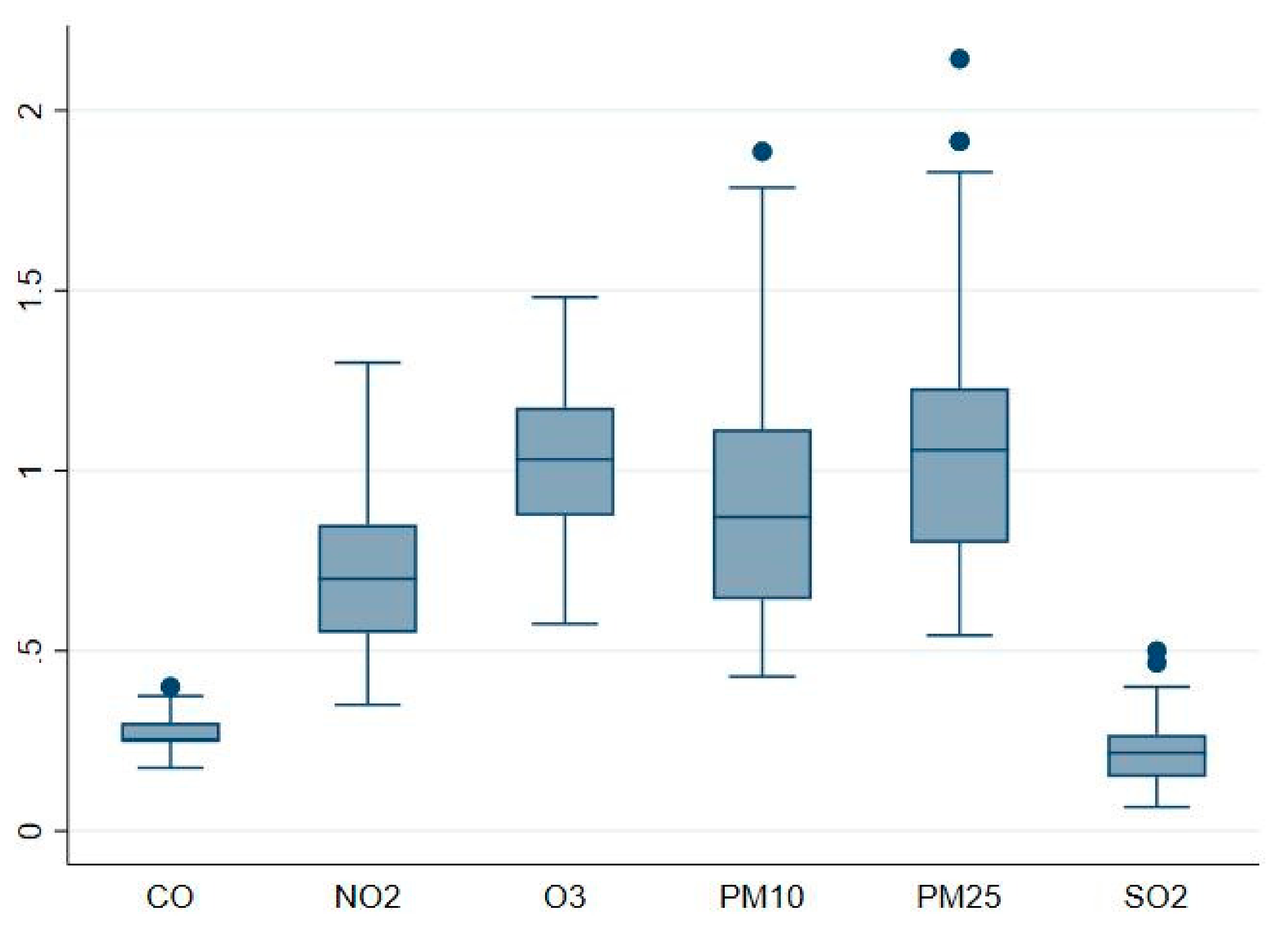
Table 1 reports the summary statistics data used in the regressions and the corresponding data sources. The average of self-reported physical and mental health is 3.12/5 and 22.91/30, respectively. For both health indicators, a higher score suggests a better health status. The income of older adults is 66% of the average income in respective areas (rural or urban) at the province level. The variable income is calculated as the summation of the income from wage, self-employment, capital, pension, and government transfer. Among the income sources, capital income is negative for some respondents. As a result, 24 respondents have relative income as negative in the sample. The average age of respondents in the sample is 62. We also included the city-level average density of each pollutant in the month when respondents were interviewed in Table 1. Since the densities across pollutants are not directly comparable, we compute pollutant-specific indexes by taking the ratio between actual pollutant density and its corresponding national level-2 density limit. These unit-free measurements allow us to compare the pollution levels across different pollutants, and the impact of each pollutant on mental health. As shown in Table 1 and Figure 1, PM2.5, PM10 and O3 appear to be the more severe pollutants: the indexes are above or close to one, suggesting on average, the air pollution levels exceed or close to the national standards. PM2.5 and PM10 indexes show substantial variations with a positive skewness: Many counties have particularly high densities of PM2.5 and PM10. On the other hand, SO2 and CO pollution levels are well below the standards with limited variations, thus are less of concern across counties. The SPI is calculated as the summation of the six unit-free pollutant indexes, indicating the overall air pollution level in a city.
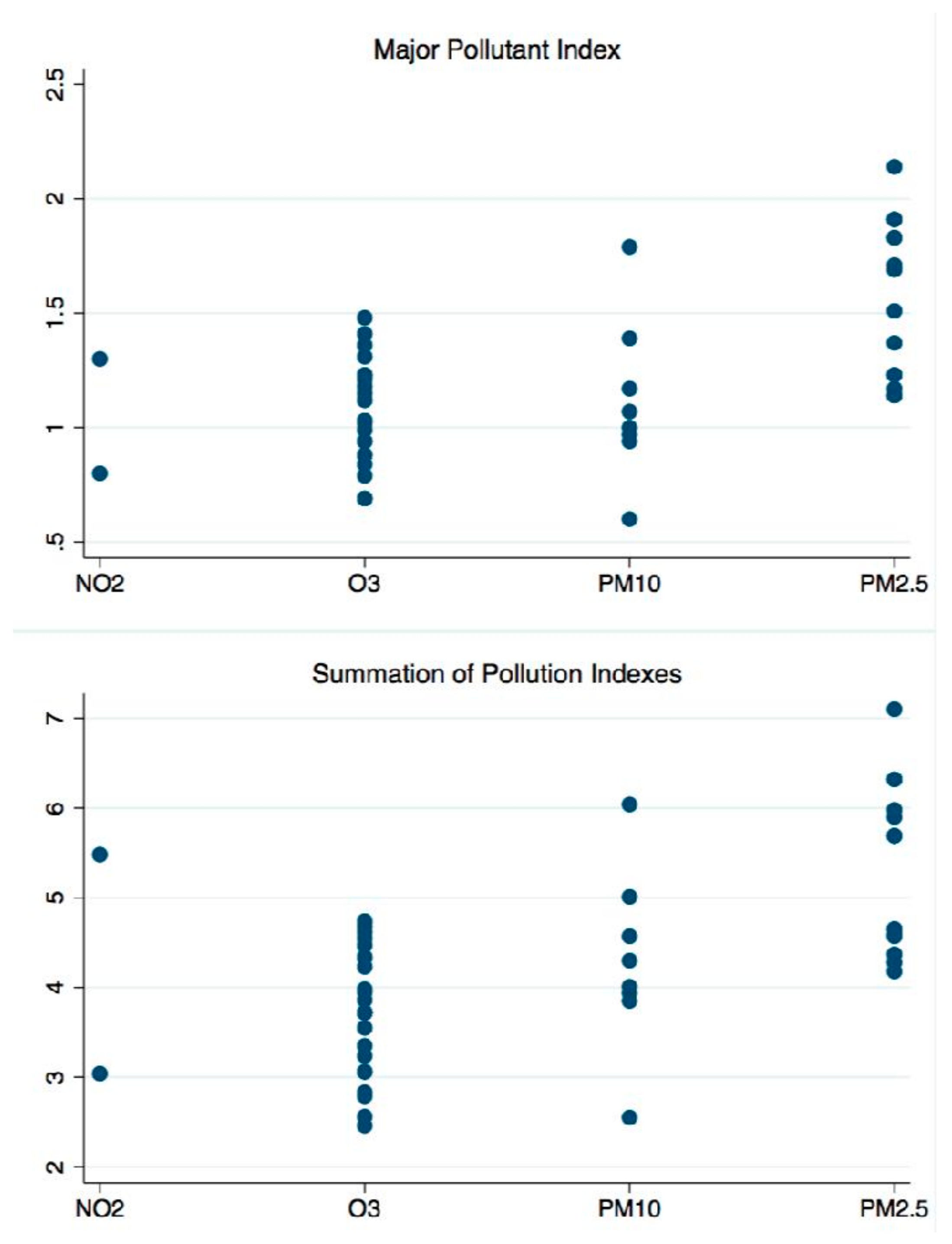
We define the major pollutant index (MPI) as the highest of the six individual pollutant indexes in a county, i.e., the index of the most polluting pollutant in reference to the national standard limits. The major pollutant is very likely to draw the deepest concerns from the locals. Figure 2 shows the scatter plot of the county-level MPI and SPI by major pollutant type. SO2 and CO are not the major pollutants for any counties in the sample. Consistent with Table 1, PM2.5, PM10, and O3 are the major pollutants in 47 of the 49 counties. O3 is the major pollutant for 25 counties; these counties generally have less air pollution and lower air quality indexes. Conversely, counties with either PM2.5 or PM10 as the major pollutant have a high average SPI, i.e., more polluting counties tend to have higher densities of PM2.5 and PM10. This helps to explain why the particulate matter is the main concern of air pollution nationwide in China. Overall, counties with a high index for the major pollutant also have a high overall pollution level. The correlation between MPI and SPI is 0.94. The results regarding the impact of air pollution on mental health and depression are further examined and presented in the next section.
4. Results
4.1. Baseline Model
In this section, we present and discuss the estimation results of Equation (1) using ordered logit regressions. Weighting is a critical step in survey sample modeling in order to derive unbiased estimates, as argued by [22]. Nonetheless, environmental data are missing for some counties, and we hence analyze a subset of the entire sample. The weighted sample still cannot represent the population in our case, as the weights in the whole original sample become biased when we drop some counties from this study due to missing data. Therefore, estimation results with "wrong" weights led to an unfavorable interpretation for both the population and the current smaller sample. For this reason, we estimate the model without the originally assigned weights.
The main results are presented in Table 2, Table 3, Table 4, and Table 5. We used month fixed effects in all estimations to capture the unobservable variations across months. All standard errors in the parentheses are robust to heteroscedasticity. In each table, the columns with odd numbers include regional fixed effects while columns with even numbers do not. In general, we found little variations in terms of economic and statistical significance, indicating the results are robust to change in model specifications. Table 2 presents the impacts of SPI and MPI on mental health and depression. Although negatively correlated with mental health, we find no statistically significant evidence between the pollution indexes and mental health. This is likely because that many questions measuring mental health are not directly relevant to air pollution. Depression level, however, is higher in counties with higher SPI and MPI. The coefficient of MPI is higher than it of SPI, suggesting MPI has a stronger impact on depression than SPI. The higher impact of MPI is evidence that people generally are more sensitive to the aggravation of major air pollutants, compared to other pollutants that have a more "acceptable" status.
Among other covariates in the model, older people tend to be less likely to be depressed. Similar results are found in Japan by [23]. However, age does not have a significant impact on overall mental health. Higher relative income is associated with good mental health but does not help to relieve depression. Females, single respondents, and those who live in rural areas exhibit poor mental health and more significant depression. Not surprisingly, better physical health conditions, more social contacts, and more living (less deceased) children lead to a higher score of mental health and less depression. Having a child co-residing or nearby does not significantly affect the mental health and depression of older adults. This is potentially due to the double-edged effects of children’s support. On the one hand, with family still being the principal institution for support of older adults in China [24], living with or near children can significantly improve elderly welfare [25]. On the other hand, older adults may experience diminished control over their lives as children take over the responsibilities, thus hurting self-esteem [26].
Table 3, Table 4 and Table 5 present the effects of each individual air pollutant on older adults’ overall mental health and depression. We estimate the effects for different pollutants in separate ordered logit regressions, given that indexes are highly positively correlated (Table 6). For example, counties with high indexes of PM2.5 are likely to have more PM10 pollution as well, and the correlation is 0.93. Including all indexes in one estimation could potentially lead to collinearity issues. Since all pollution densities are normalized to unit−free pollutant indexes according to the respective limit standards, the magnitudes of coefficients across pollutant indexes are directly comparable. The coefficients of control variables exhibit little variations from Table 3 to Table 5. Although negatively correlated with mental health, the results show that most indexes have no clear impact on overall mental health. This is again due to the irrelevancy between air pollution and many factors measuring mental health. For the NO2 index, we find it counter−intuitive that mental health improves as the index increases.
The coefficients of pollutant indexes with depression as the dependent variable are of particular interests. PM2.5 and PM10 are the representative air pollutants: Both show an economically and statistically significant correlation with depression. Respondents living in counties with high particulate matter densities are likely to have high levels of depression. Although not a major pollutant in any counties, the SO2 index is also positively related to depression with a high magnitude. One possible explanation for the high magnitude of the SO2 coefficient is its low index level (Figure 1). Therefore, any small change in the index could lead to a relatively significant impact. We will further examine this issue later. No similar evidence is found for O3, NO2, and CO: a high level of any of these pollutant indexes does not lead to more depression. Although O3 is the major pollutant in half of the counties and the average of O3 index is high, the variation is low. This is also true for NO2 and CO indexes: compared to pollutants with significant impacts on depression, O3, NO2 and CO indexes have lower coefficients of variation, which is defined as the ratio of the standard deviation to the mean (Table 7). The results indicate that people are more concerned about environmental inequalities rather than the absolute pollution level, i.e., whether the local air pollution is significantly higher than the national average. Another possible explanation for the insignificant impact of O3 is its invisibility. Unlike particulate matter, O3 is hardly perceived by the general public and thus raises much less concern.
4.2. Robustness Check
In this section, we test alternative model specifications to check the robustness of the main results. Since the coefficients of control covariates are consistent from Table 2 to Table 5, we include them in every regression but omit them from the results. As shown in the previous session, respondents are more sensitive to the air pollution disparity, not the magnitude of the pollution indexes. Moreover, one can easily change the index of a pollutant by altering its national density limit. Therefore, for county i, we replace each pollutant index by relative pollutant index, which is defined as (Pollutant indexi − National average pollutant index)/ National average pollutant index. Thus, the relative pollutant index is free of the national limit set by the regulator and directly compares local air pollution to the national average.
As illustrated in Table 8, all results show similar signs and statistical significance comparing to the baseline model. The major difference comes from SO2 and CO: the coefficients are much smaller compared to those presented in Table 5. The low coefficients indicate that because of the particularly loose national standard limits for these two pollutants, using the pollutant indexes directly (instead of the relative pollutant indexes) causes an upward bias of the estimates. In this situation, people care less about the standard limits as the indexes are low everywhere. Rather, it raises more concerns when the local pollution level is high comparing with reference counties, regardless of the magnitude. We also estimate the model with each pollutant’s density. As shown in Table 8, the results exhibit little deviation from the baseline model, justifying the robustness of our major findings.
Some of the survey questions described above are related to depression, namely Questions (1), (2), (6), (7), and (10). We broaden the definition of the dependent variable "depression" by including these questions in the calculation, along with Question (3). Therefore, the broad definition of depression is a six−item summation ranging from 0 to 18, with higher scores indicating a more severe depression status. The estimation results are presented at the bottom of Table 8. Overall the results are consistent with those derived from the main model, suggesting air pollution as a potential interpretation for various symptoms related to depression. Note that the statistical significance becomes weaker. The reduction in statistical significance is almost inevitable due to the fact that, as more questions are included, so are noises.
5. Conclusions and Discussion
As a result of the rapid economic development and industrialization, the issues about both air pollution and population aging have emerged in China. In this paper, we investigate the factors associated with the mental health and depression of older adults in China with an emphasis on air pollution. Due to its visibility, air pollution may serve as a primary surrogate of the byproducts of urbanization, raising public concern nationwide. Another potential factor that links air pollution and subjective well−being is physical health. Exposure to air pollution increases more tangible health risks, resulting in deteriorated mental health [16,27]. In addition, air quality is an important local public good [12]. A fall in the value of this public good caused by air pollution impairs the stated well−being.
Although we find no strong relationship between air pollution and overall mental health, both poor overall air quality and high major pollutant density are associated with a higher level of depression. Environmental inequality is one of the main driving forces of depression. Among the six individual pollutants, we find that peoples are most sensitive to PM2.5, PM10, and SO2, i.e., pollutants with a high discrepancy in densities across counties. Although the absolute density is high compared with the national standard limit, the impact of O3 on mental health is low due to its limited variations nationwide. Our main findings also show females, single older adults, and those who live in a rural area and with less living children exhibit poor mental health and more significant depression.
There are a few caveats to our analyses that should be noted. First, comparing with panel data, the cross−sectional data refrain us from controlling the unobservable variations at the individual level in this study. To alleviate this issue, socioeconomic variables, as well as location fixed effects, are included in the model to help to characterize respondents. Second, weighted estimation is not applicable as the sample in this study is only a subset of the entire survey due to the lack of environmental data for some counties. Therefore, one should be cautious when interpreting and generalizing the conclusions to the entire population. Lastly, despite its insignificance comparing with other pollutants, the positive relation between the NO2 index and mental health remains contradictory and needs to be further explored in future research.
Author Contributions
Conceptualization, Y.Z. and J.L.; methodology, Y.Z.; software, Y.Z.; validation, Y.Z. and J.L.; formal analysis, Y.Z. and J.L.; investigation, Y.Z. and J.L.; resources, Y.Z. and J.L.; data curation, Y.Z. and J.L.; writing—original draft preparation, Y.Z. and J.L.; writing—review and editing, Y.Z. and J.L.; visualization, Y.Z.; supervision, Y.Z. All authors have read and agreed to the published version of the manuscript.
Funding
This research received no external funding.
Conflicts of Interest
The authors declare no conflict of interest.
References
- Szreter, S. Rapid economic growth and the four ds of disruption, deprivation, disease and death: Public health lessons from nineteenth−century britain for twenty−first−century China? Trop. Med. Int. Health 1999, 4, 146–152. [Google Scholar] [CrossRef] [PubMed] [Green Version]
- Helliwell, J.F.; Huang, H. How’s your government? International evidence linking good government and well−being. Br. J. Political Sci. 2008, 38, 595–619. [Google Scholar] [CrossRef] [Green Version]
- Williams, L.; Zhang, R.; Packard., K.C. Factors affecting the physical and mental health of older adults in china: The importance of marital status, child proximity, and gender. Ssm Popul. Health 2017, 3, 20–36. [Google Scholar] [CrossRef] [PubMed]
- Rohde, N.; Tang, K.K.; Osberg, L.; Rao, P. The effect of economic insecurity on mental health: Recent evidence from australian panel data. Soc. Sci. Med. 2016, 151, 250–258. [Google Scholar] [CrossRef] [Green Version]
- Madianos, M.; Economou, M.; Alexiou, T.; Stefanis, C. Depression and economic hardship across greece in 2008 and 2009: Two cross−sectional surveys nationwide. Soc. Psychiatry Psychiatric Epidemiology 2011, 46, 943–952. [Google Scholar] [CrossRef]
- Graham, C.; Higuera, L.; Lora, E. Which health conditions cause the most unhappiness? Health Econ. 2011, 20, 1431–1447. [Google Scholar] [CrossRef]
- Allen, J.; Balfour, R.; Bell, R.; Marmot, M. Social determinants of mental health. Int. Rev. Psychiatry 2014, 26, 392–407. [Google Scholar] [CrossRef]
- Brockmann, H.; Delhey, J.; Welzel, C.; Yuan, H. The china puzzle: Falling happiness in a rising economy. J. Happiness Stud. 2009, 10, 387–405. [Google Scholar] [CrossRef]
- Graham, C.; Zhou, S.; Zhang, J. Happiness and health in China: The paradox of progress. World Dev. 2017, 96, 231–244. [Google Scholar] [CrossRef]
- Wang, Q.; Tapia Granados, J.A. Economic growth and mental health in 21st century China. Soc. Sci. Med. 2019, 220, 387–395. [Google Scholar] [CrossRef]
- Ferreira, S.; Akay, A.; Brereton, F.; Cuñado, J.; Martinsson, P.; Moro, M.; Ningal, T.F. Life satisfaction and air quality in Europe. Ecol. Econ. 2013, 88, 1–10. [Google Scholar] [CrossRef]
- Levinson, A. Valuing public goods using happiness data: The case of air quality. J. Public Econ. 2012, 96, 869–880. [Google Scholar] [CrossRef]
- Luechinger, S. Valuing air quality using the life satisfaction approach. Econ. J. 2009, 119, 482–515. [Google Scholar] [CrossRef]
- Luechinger, S. Life satisfaction and transboundary air pollution. Econ. Lett. 2010, 107, 4–6. [Google Scholar] [CrossRef]
- Menz., T. Do people habituate to air pollution? Evidence from international life satisfaction data. Ecol. Econ. 2011, 71, 211–219. [Google Scholar] [CrossRef]
- Zhang, X.; Zhang, X.; Chen, X. Happiness in the air: How does a dirty sky affect mental health and subjective well−being? J. Environ. Econ. Manag. 2017, 85, 81–94. [Google Scholar] [CrossRef]
- Nandita, B. Slum upgrading strategies involving physical environment and infrastructure interventions and their effects on health and socio-economic outcomes. J. Evid.Based Med. 2013, 6, 57. [Google Scholar]
- Easterlin, R.A. Does economic growth improve the human lot? Some empirical evidence. Nations Househ. Econ. Growth 1974, 1, 89–125. [Google Scholar]
- Easterlin, R.A. Will raising the incomes of all increase the happiness of all? J. Econ. Behav. Organ. 1995, 27, 35–47. [Google Scholar] [CrossRef]
- Ren, Q.; Ye, M. Losing children and mental well−being: Evidence from China. Appl. Econ. Lett. 2017, 24, 868–877. [Google Scholar] [CrossRef]
- Grundy, E.; van Campen, C.; Deeg, D.; Dourgnon, P.; Huisman, M.; Ploubidis, G.; Tsim-bos, C. Health Inequalities and the Health Divide among Older People in the Who European Region: The European Review on the Social Determinants of Health and the Health Divide (Report of the Task Group on Older People); World Health Organization: Copenhagen, Denmark, 2013. [Google Scholar]
- Lavallée, P.; Beaumont, J.-F. Why we should put some weight on weights. Surv. Methods Insights Field Smif 2015. [Google Scholar] [CrossRef]
- Donovan, N.; Halpern, D.; Sargeant, R. Life Satisfaction: The State of Knowledge and Implications for Government; Cabinet Office/Strategy Unit: London, UK, 2002. [Google Scholar]
- Yi, Z.; Wang, Z. Dynamics of family and elderly living arrangements in china: New lessons learned from the 2000 census. China Rev. 2003, 3, 95–119. [Google Scholar]
- Knodel, J.; Debavalya, N. Living arrangements and support among the elderly in south−east asia: An introduction. Asia Pac. Popul. J. 1997, 12, 5–16. [Google Scholar] [CrossRef]
- Umberson, D.; Pudrovska, T.; Reczek, C. Parenthood, childlessness, and well−being: A life course perspective. J. Marriage Fam. 2010, 72, 612–629. [Google Scholar] [CrossRef] [Green Version]
- Greenstone, M.; Hanna, R. Environmental regulations, air and water pollution, and infant mortality in India. Am. Econ. Rev. 2014, 104, 3038–3072. [Google Scholar] [CrossRef] [Green Version]
Figure 1.
Box plot of pollutant indexes.

Figure 2.
Major pollutant index (MPI) and summation of pollution indexes (SPI) by major pollutant type.
Figure 2.
Major pollutant index (MPI) and summation of pollution indexes (SPI) by major pollutant type.


Table 1.
Summary Statistics: Year 2015.
| Variables | Mean | Std. Dev. | Min. | Max. |
|---|---|---|---|---|
| CHARLS | ||||
| Mental health | 22.91 | 5.82 | 0 | 30 |
| Depression | 0.72 | 1.02 | 0 | 3 |
| Physical health | 3.12 | 0.95 | 1 | 5 |
| Age | 62.03 | 9.35 | 45 | 93 |
| Relative income | 0.66 | 1.20 | −4.65 | 16.62 |
| Female | 0.53 | 0 | 1 | |
| Marital status | 0.83 | 0 | 1 | |
| Living children ratio | 0.96 | 0.15 | 0 | 1 |
| Co-residing child | 0.53 | 0 | 1 | |
| Nearby child | 0.87 | 0 | 1 | |
| Rural | 0.51 | 0 | 1 | |
| Social contacts | 0.51 | 0 | 1 | |
| # of Observations | 3406 | |||
| CNEMC | ||||
| PM2.5 | 38.41 | 14.13 | 19 | 75 |
| PM10 | 67.67 | 26.12 | 30 | 132 |
| O3 | 165.49 | 33.32 | 92 | 237 |
| SO2 | 13.61 | 5.74 | 4 | 30 |
| NO2 | 28.57 | 8.92 | 14 | 52 |
| CO | 1.09 | 0.20 | 0.7 | 1.6 |
| Summation of pollution indexes (SPI) | 4.31 | 1.07 | 2.46 | 7.10 |
| Major pollutant index (MPI) | 1.21 | 0.36 | 0.60 | 2.14 |
| PM2.5 index | 1.10 | 0.40 | 0.54 | 2.14 |
| PM10 index | 0.96 | 0.37 | 0.43 | 1.89 |
| O3 index | 1.03 | 0.21 | 0.58 | 1.48 |
| SO2 index | 0.23 | 0.10 | 0.07 | 0.50 |
| NO2 index | 0.71 | 0.22 | 0.35 | 1.30 |
| CO index | 0.27 | 0.05 | 0.18 | 0.40 |
| # of Counties | 49 |
The units of measurement are µg/m3 for PM2.5, PM10, O3, SO2, and NO2, and mg/m3 for CO.
Table 2.
Impacts of SPI and MPI on mental health and depression.
| Dependent Variable | SPI | MPI | ||||||
|---|---|---|---|---|---|---|---|---|
| Mental Health | Depression | Mental Health | Depression | |||||
| (1) | (2) | (3) | (4) | (5) | (6) | (7) | (8) | |
| SPI | −0.002 | −0.014 | 0.085* | 0.099*** | ||||
| (0.037) | (0.026) | (0.045) | (0.030) | |||||
| MPI | −0.036 | 0.005 | 0.300** | 0.247*** | ||||
| (0.126) | (0.078) | (0.153) | (0.090) | |||||
| Age | 0.001 | 0.001 | −0.010** | −0.010** | 0.001 | 0.001 | −0.010** | −0.010** |
| (0.004) | (0.004) | (0.004) | (0.004) | (0.004) | (0.004) | (0.004) | (0.004) | |
| Relative Income | 0.066** | 0.066** | −0.006 | −0.005 | 0.066** | 0.067** | −0.004 | −0.005 |
| (0.027) | (0.026) | (0.027) | (0.027) | (0.027) | (0.026) | (0.027) | (0.027) | |
| Female | −0.426*** | −0.418*** | 0.384*** | 0.378*** | −0.427*** | −0.418*** | 0.385*** | 0.378*** |
| (0.063) | (0.063) | (0.072) | (0.072) | (0.063) | (0.063) | (0.072) | (0.072) | |
| Married | 0.475*** | 0.466*** | −0.234** | −0.225** | 0.475*** | 0.464*** | −0.232** | −0.221** |
| (0.085) | (0.085) | (0.095) | (0.095) | (0.085) | (0.085) | (0.095) | (0.095) | |
| Physical Health | 0.724*** | 0.740*** | −0.594*** | −0.607*** | 0.724*** | 0.740*** | −0.594*** −0.608*** | |
| (0.035) | (0.034) | (0.045) | (0.044) | (0.035) | (0.034) | (0.045) | (0.045) | |
| Living Children Ratio | 0.650*** | 0.713*** | −0.419* | −0.470* | 0.651*** | 0.715*** | −0.419* | −0.471* |
| (0.214) | (0.217) | (0.247) | (0.246) | (0.214) | (0.217) | (0.246) | (0.246) | |
| Co-residing Child | 0.026 | 0.008 | −0.003 | 0.012 | 0.026 | 0.010 | −0.005 | 0.010 |
| (0.068) | (0.068) | (0.081) | (0.080) | (0.068) | (0.068) | (0.081) | (0.080) | |
| Nearby Child | 0.143 | 0.152 | −0.147 | −0.152 | 0.143 | 0.151 | −0.147 | −0.151 |
| (0.101) | (0.102) | (0.119) | (0.118) | (0.101) | (0.102) | (0.119) | (0.118) | |
| Rural | −0.334*** | −0.330*** | 0.233*** | 0.234*** | −0.332*** | −0.330*** | 0.213*** | 0.218*** |
| (0.065) | (0.064) | (0.077) | (0.077) | (0.065) | (0.065) | (0.078) | (0.077) | |
| Social Contacts | 0.245*** | 0.246*** | −0.088 | −0.086 | 0.246*** | 0.244*** | −0.090 | −0.085 |
| (0.062) | (0.062) | (0.071) | (0.071) | (0.062) | (0.062) | (0.071) | (0.071) | |
| Regional FE | Yes | No | Yes | No | Yes | No | Yes | No |
Month fixed effects in all specifications. Robust standard errors in parentheses.***: p < 1%, **: p < 5%, *: p < 10%.
Table 3.
Impacts of PM2.5 and PM10 on mental health and depression.
| Dependent Variable | PM2.5 | Index | PM10 | Index | ||||
|---|---|---|---|---|---|---|---|---|
| Mental Health | Depression | Mental Health | Depression | |||||
| (1) | (2) | (3) | (4) | (5) | (6) | (7) | (8) | |
| PM2.5 Index | −0.081 | −0.037 | 0.309** | 0.267*** | ||||
| (0.105) | (0.068) | (0.122) | (0.078) | |||||
| PM10 Index | −0.176 | −0.080 | 0.359** | 0.308*** | ||||
| (0.120) | (0.077) | (0.142) | (0.087) | |||||
| Age | 0.001 | 0.001 | −0.010** | −0.010** | 0.001 | 0.001 | −0.010** | −0.010** |
| (0.004) | (0.004) | (0.004) | (0.004) | (0.004) | (0.004) | (0.004) | (0.004) | |
| Relative Income | 0.065** | 0.066** | −0.003 | −0.003 | 0.064** | 0.065** | −0.003 | −0.004 |
| (0.027) | (0.026) | (0.027) | (0.027) | (0.027) | (0.026) | (0.027) | (0.027) | |
| Female | -0.427*** | −0.418*** | 0.386*** | 0.379*** | −0.427*** | −0.418*** | 0.385*** | 0.378*** |
| (0.063) | (0.063) | (0.072) | (0.072) | (0.063) | (0.063) | (0.072) | (0.072) | |
| Married | 0.474*** | 0.465*** | −0.229** | −0.220** | 0.475*** | 0.467*** | −0.232** | −0.223** |
| (0.085) | (0.085) | (0.095) | (0.095) | (0.085) | (0.085) | (0.095) | (0.095) | |
| Physical Health | 0.725*** | 0.740*** | −0.596*** | −0.609*** | 0.725*** | 0.740*** | −0.595*** −0.607*** | |
| (0.035) | (0.034) | (0.045) | (0.045) | (0.035) | (0.034) | (0.045) | (0.045) | |
| Living Children Ratio | 0.654*** | 0.715*** | −0.431* | −0.478* | 0.659*** | 0.714*** | −0.426* | −0.474* |
| (0.214) | (0.217) | (0.246) | (0.245) | (0.213) | (0.217) | (0.245) | (0.245) | |
| Co-residing Child | 0.026 | 0.008 | −0.007 | 0.011 | 0.025 | 0.005 | −0.004 | 0.015 |
| (0.068) | (0.068) | (0.081) | (0.080) | (0.068) | (0.068) | (0.081) | (0.080) | |
| Nearby Child | 0.143 | 0.153 | −0.151 | −0.158 | 0.143 | 0.154 | −0.147 | −0.154 |
| (0.101) | (0.102) | (0.119) | (0.118) | (0.101) | (0.102) | (0.119) | (0.118) | |
| Rural | −0.331*** | −0.327*** | 0.215*** | 0.216*** | −0.336*** | −0.329*** | 0.232*** | 0.231*** |
| (0.065) | (0.064) | (0.078) | (0.077) | (0.065) | (0.064) | (0.077) | (0.077) | |
| Social Contacts | 0.248*** | 0.246*** | −0.090 | −0.085 | 0.250*** | 0.247*** | −0.090 | −0.085 |
| (0.062) | (0.062) | (0.071) | (0.071) | (0.062) | (0.062) | (0.071) | (0.071) | |
| Regional FE | Yes | No | Yes | No | Yes | No | Yes | No |
Month fixed effects in all specifications. Robust standard errors in parentheses. ***: p < 1%, **: p < 5%, *: p < 10%.
Table 4.
Impacts of O3 and NO2 on mental health and depression.
| Dependent Variable | O3 Index | NO2 | Index | |||||
|---|---|---|---|---|---|---|---|---|
| Mental Health | Depression | Mental Health | Depression | |||||
| (1) | (2) | (3) | (4) | (5) | (6) | (7) | (8) | |
| O3 Index | 0.220 | 0.222 | 0.038 | 0.078 | ||||
| (0.180) | (0.153) | (0.201) | (0.172) | |||||
| NO2 Index | 0.437** | −0.061 | −0.109 | 0.358** | ||||
| (0.172) | (0.131) | (0.202) | (0.152) | |||||
| Age | 0.001 | 0.001 | −0.010** | −0.011** | 0.001 | 0.001 | −0.010** | −0.011** |
| (0.004) | (0.004) | (0.004) | (0.004) | (0.004) | (0.004) | (0.004) | (0.004) | |
| Relative Income | 0.066** | 0.067** | −0.008 | −0.008 | 0.064** | 0.067** | −0.007 | −0.009 |
| (0.027) | (0.026) | (0.027) | (0.027) | (0.027) | (0.026) | (0.027) | (0.027) | |
| Female | −0.426*** | −0.417*** | 0.383*** | 0.377*** | −0.428*** | −0.418*** | 0.383*** | 0.378*** |
| (0.063) | (0.063) | (0.072) | (0.072) | (0.063) | (0.063) | (0.072) | (0.072) | |
| Married | 0.474*** | 0.460*** | −0.235** | −0.218** | 0.472*** | 0.466*** | −0.233** | −0.226** |
| (0.085) | (0.085) | (0.095) | (0.095) | (0.085) | (0.085) | (0.095) | (0.095) | |
| Physical Health | 0.725*** | 0.739*** | −0.592*** | −0.608*** | 0.722*** | 0.739*** | −0.592*** −0.606*** | |
| (0.035) | (0.034) | (0.045) | (0.045) | (0.035) | (0.034) | (0.045) | (0.045) | |
| Living Children Ratio | 0.649*** | 0.716*** | −0.397 | −0.463 | 0.655*** | 0.709*** | −0.395 | −0.440* |
| (0.214) | (0.216) | (0.247) | (0.247) | (0.214) | (0.217) | (0.247) | (0.246) | |
| Co−residing Child | 0.026 | 0.015 | −0.002 | −0.004 | 0.017 | 0.011 | −0.001 | −0.012 |
| (0.068) | (0.068) | (0.081) | (0.080) | (0.068) | (0.068) | (0.081) | (0.080) | |
| Nearby Child | 0.149 | 0.155 | −0.148 | −0.139 | 0.145 | 0.151 | −0.149 | −0.146 |
| (0.101) | (0.102) | (0.118) | (0.118) | (0.101) | (0.102) | (0.118) | (0.118) | |
| Rural | −0.335*** | −0.332*** | 0.229*** | 0.234*** | −0.291*** | −0.335*** | 0.220*** | 0.265*** |
| (0.065) | (0.064) | (0.077) | (0.076) | (0.067) | (0.065) | (0.079) | (0.078) | |
| Social Contacts | 0.240*** | 0.239*** | −0.083 | −0.081 | 0.243*** | 0.245*** | −0.082 | −0.082 |
| (0.062) | (0.062) | (0.071) | (0.071) | (0.062) | (0.062) | (0.071) | (0.071) | |
| Regional FE | Yes | No | Yes | No | Yes | No | Yes | No |
Month fixed effects in all specifications. Robust standard errors in parentheses. ***: p < 1%, **: p < 5%, *: p < 10%.
Table 5.
Impacts of SO2 and CO on mental health and depression.
| Dependent Variable | SO2 | Index | CO Index | |||||
|---|---|---|---|---|---|---|---|---|
| Mental Health | Depression | Mental Health | Depression | |||||
| (1) | (2) | (3) | (4) | (5) | (6) | (7) | (8) | |
| SO2 Index | −0.368 | −0.249 | 0.785** | 0.837** | ||||
| (0.320) | (0.297) | (0.364) | (0.336) | |||||
| CO Index | −0.040 | −0.828 | −0.191 | 0.957 | ||||
| (0.634) | (0.572) | (0.694) | (0.636) | |||||
| Age | 0.001 | 0.001 | −0.010** | −0.011** | 0.001 | 0.001 | −0.010** | −0.010** |
| (0.004) | (0.004) | (0.004) | (0.004) | (0.004) | (0.004) | (0.004) | (0.004) | |
| Relative Income | 0.066** | 0.066** | −0.008 | −0.008 | 0.066** | 0.067** | −0.008 | −0.008 |
| (0.027) | (0.026) | (0.027) | (0.027) | (0.027) | (0.026) | (0.027) | (0.027) | |
| Female | −0.427*** | −0.418*** | 0.382*** | 0.375*** | −0.426*** | −0.420*** | 0.383*** | 0.379*** |
| (0.063) | (0.063) | (0.072) | (0.072) | (0.063) | (0.063) | (0.072) | (0.072) | |
| Married | 0.474*** | 0.464*** | −0.232** | −0.216** | 0.475*** | 0.465*** | −0.234** | −0.219** |
| (0.085) | (0.085) | (0.095) | (0.095) | (0.085) | (0.085) | (0.095) | (0.095) | |
| Physical Health | 0.726*** | 0.741*** | −0.596*** | −0.611*** | 0.724*** | 0.739*** | −0.593*** −0.605*** | |
| (0.035) | (0.034) | (0.045) | (0.044) | (0.035) | (0.034) | (0.045) | (0.045) | |
| Living Children Ratio | 0.661*** | 0.723*** | −0.427* | −0.498** | 0.649*** | 0.701*** | −0.397 | −0.449* |
| (0.213) | (0.216) | (0.247) | (0.248) | (0.214) | (0.218) | (0.246) | (0.248) | |
| Co−residing Child | 0.021 | 0.005 | 0.006 | 0.010 | 0.026 | 0.004 | −0.004 | 0.000 |
| (0.068) | (0.068) | (0.081) | (0.080) | (0.068) | (0.068) | (0.081) | (0.080) | |
| Nearby Child | 0.143 | 0.151 | −0.146 | −0.140 | 0.143 | 0.154 | −0.148 | −0.144 |
| (0.101) | (0.102) | (0.118) | (0.118) | (0.101) | (0.102) | (0.119) | (0.118) | |
| Rural | −0.334*** | −0.330*** | 0.225*** | 0.233*** | −0.335*** | −0.341*** | 0.227*** | 0.248*** |
| (0.065) | (0.064) | (0.077) | (0.077) | (0.066) | (0.065) | (0.077) | (0.077) | |
| Social Contacts | 0.245*** | 0.244*** | −0.082 | −0.078 | 0.245*** | 0.245*** | −0.082 | −0.079 |
| (0.061) | (0.061) | (0.071) | (0.071) | (0.061) | (0.062) | (0.071) | (0.071) | |
| Regional FE | Yes | No | Yes | No | Yes | No | Yes | No |
Month fixed effects in all specifications. Robust standard errors in parentheses. ***: p < 1%, **: p < 5%, *: p < 10%.
Table 6.
Correlations between pollutant indexes.
| PM2.5 | PM10 | O3 | SO2 | NO2 | CO | |
|---|---|---|---|---|---|---|
| PM2.5 | 1.000 | |||||
| PM10 | 0.931 | 1.000 | ||||
| O3 | 0.546 | 0.466 | 1.000 | |||
| SO2 | 0.533 | 0.511 | 0.411 | 1.000 | ||
| NO2 | 0.428 | 0.463 | 0.315 | 0.181 | 1.000 | |
| CO | 0.202 | 0.307 | 0.392 | 0.349 | 0.492 | 1.000 |
p−value less than 1% for all correlations.
Table 7.
Coefficient of variation.
| PM2.5 Index | PM10 Index | SO2 Index |
|---|---|---|
| 0.38 | 0.39 | 0.42 |
| O3 index | NO2 index | CO index |
| 0.19 | 0.34 | 0.22 |
Table 8.
Robustness check.
| Relative Pollutant Index | Pollutant Density | |||||||
|---|---|---|---|---|---|---|---|---|
| Mental Health | Depression | Mental Health | Depression | |||||
| (1) | (2) | (3) | (4) | (5) | (6) | (7) | (8) | |
| PM2.5 | −0.088 | −0.041 | 0.339** | 0.294*** | −0.002 | −0.001 | 0.009** | 0.008*** |
| (0.115) | (0.075) | (0.134) | (0.085) | (0.003) | (0.002) | (0.003) | (0.002) | |
| PM10 | −0.170 | −0.077 | 0.347** | 0.297*** | −0.003 | −0.001 | 0.005** | 0.004*** |
| (0.116) | (0.074) | (0.137) | (0.084) | (0.002) | (0.001) | (0.002) | (0.001) | |
| O3 | 0.228 | 0.230 | 0.039 | 0.081 | 0.001 | 0.001 | 0.000 | 0.000 |
| (0.186) | (0.158) | (0.208) | (0.178) | (0.001) | (0.001) | (0.001) | (0.001) | |
| NO2 | 0.312** | −0.044 | −0.078 | 0.256** | 0.011** | −0.002 | −0.003 | 0.009** |
| (0.123) | (0.094) | (0.144) | (0.109) | (0.004) | (0.003) | (0.005) | (0.004) | |
| SO2 | −0.084 | −0.057 | 0.178** | 0.190** | −0.006 | −0.004 | 0.013** | 0.014** |
| (0.073) | (0.067) | (0.082) | (0.076) | (0.005) | (0.005) | (0.006) | (0.006) | |
| CO | −0.011 | −0.226 | −0.052 | 0.261 | −0.010 | −0.207 | −0.048 | 0.239 |
| (0.173) | (0.156) | (0.189) | (0.174) | (0.158) | (0.143) | (0.173) | (0.159) | |
| Regional FE | Yes | No | Yes | No | Yes | No | Yes | No |
| Dependent Variable: Broad Definition of Depression | ||||||||
| SPI | MPI | PM2.5 | PM10 | O3 | NO2 | SO2 | CO | |
| (1) | (2) | (3) | (4) | (5) | (6) | (7) | (8) | |
| 0.064* | 0.224* | 0.187* | 0.324*** | 0.041 | −0.129 | 0.611* | 0.499 | |
| (0.038) | (0.130) | (0.108) | (0.123) | (0.185) | (0.178) | (0.333) | (0.656) | |
| Regional FE | Yes | Yes | Yes | Yes | Yes | Yes | Yes | Yes |
Control covariates are included in every regression but omitted from the results. Month fixed effects in all specifications. Robust standard errors in parentheses. ***: p < 1%, **: p < 5%, *: p < 10%.
© 2020 by the authors. Licensee MDPI, Basel, Switzerland. This article is an open access article distributed under the terms and conditions of the Creative Commons Attribution (CC BY) license (http://creativecommons.org/licenses/by/4.0/).
Share and Cite
MDPI and ACS Style
Zhou, Y.; Liu, J. Air Pollution and Mental Health of Older Adults in China. Sustainability 2020, 12, 950. https://0-doi-org.brum.beds.ac.uk/10.3390/su12030950
AMA Style
Zhou Y, Liu J. Air Pollution and Mental Health of Older Adults in China. Sustainability. 2020; 12(3):950. https://0-doi-org.brum.beds.ac.uk/10.3390/su12030950
Chicago/Turabian StyleZhou, Yishu, and Jingyi Liu. 2020. "Air Pollution and Mental Health of Older Adults in China" Sustainability 12, no. 3: 950. https://0-doi-org.brum.beds.ac.uk/10.3390/su12030950
Note that from the first issue of 2016, this journal uses article numbers instead of page numbers. See further details here.