The Effects of Foreign Direct Investment, Economic Growth, Industrial Structure, Renewable and Nuclear Energy, and Urbanization on Korean Greenhouse Gas Emissions


Abstract
:1. Introduction
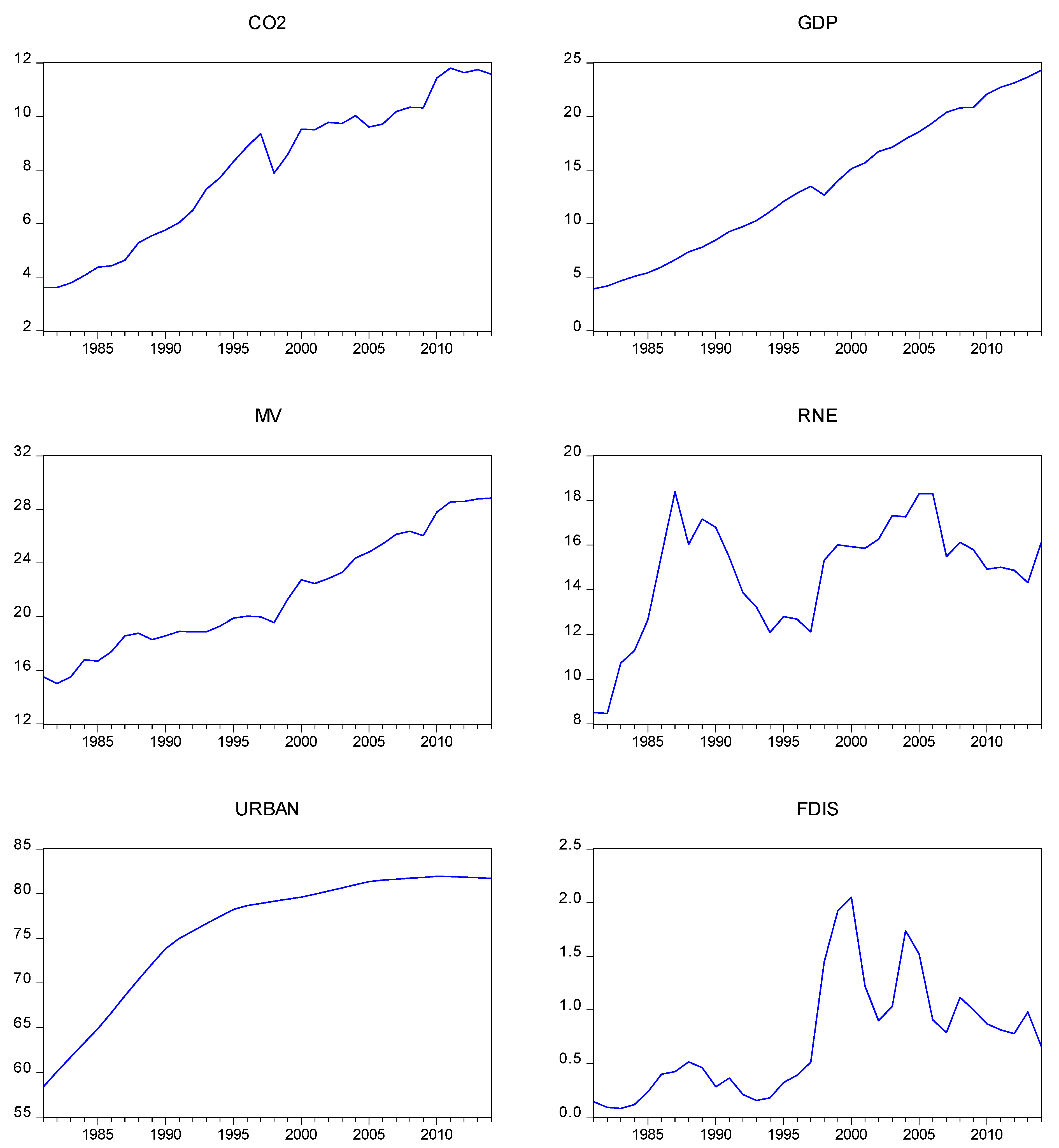
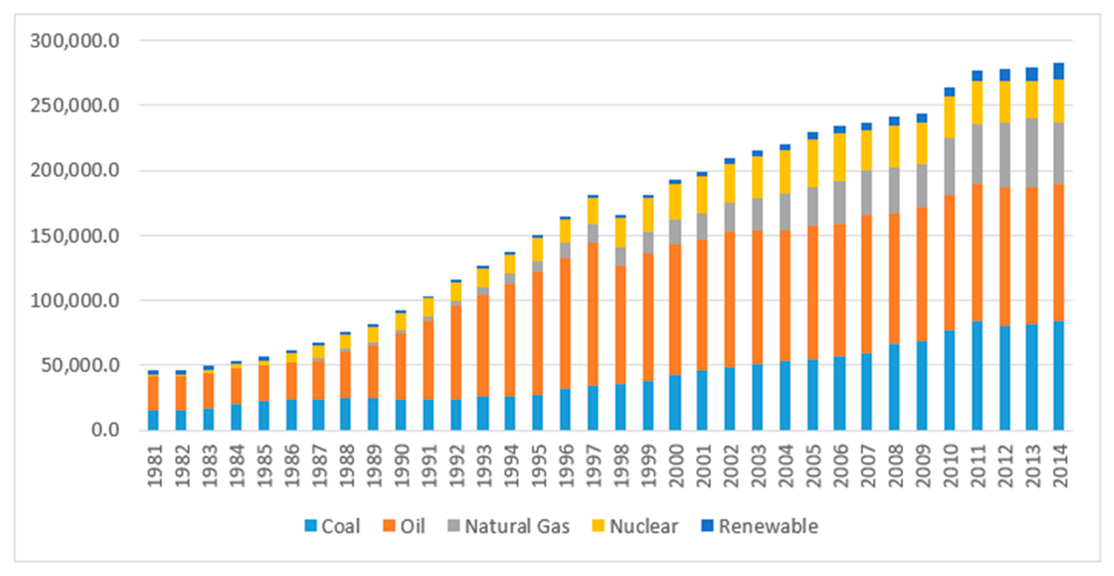
2. Data and Methods
3. Results
3.1. Unit root analysis
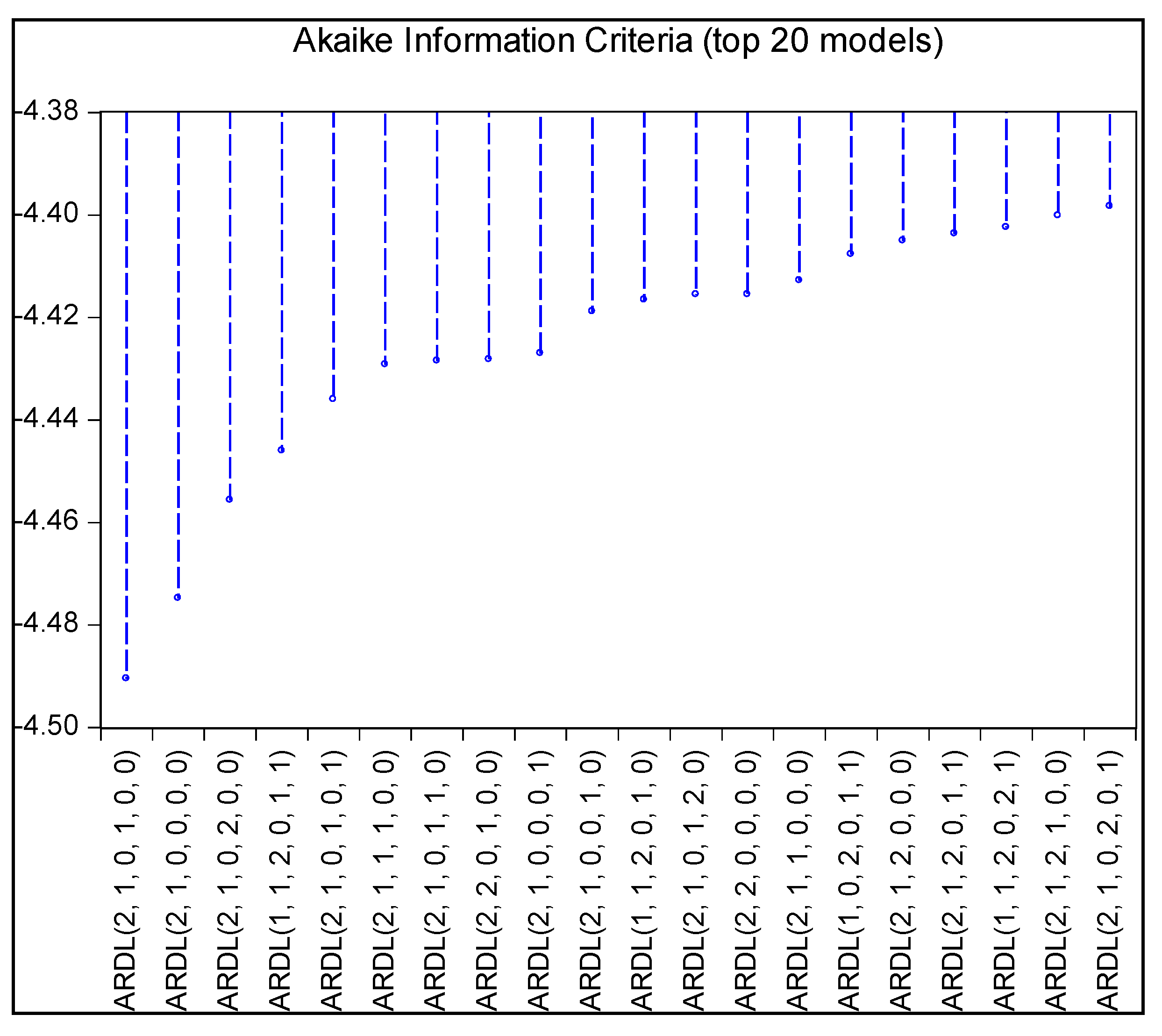
3.2. Lag Length Criteria
3.3. ARDL Bounds Tests
3.4. Long Run Equilibrium Relationship
3.5. Short-Run Causality
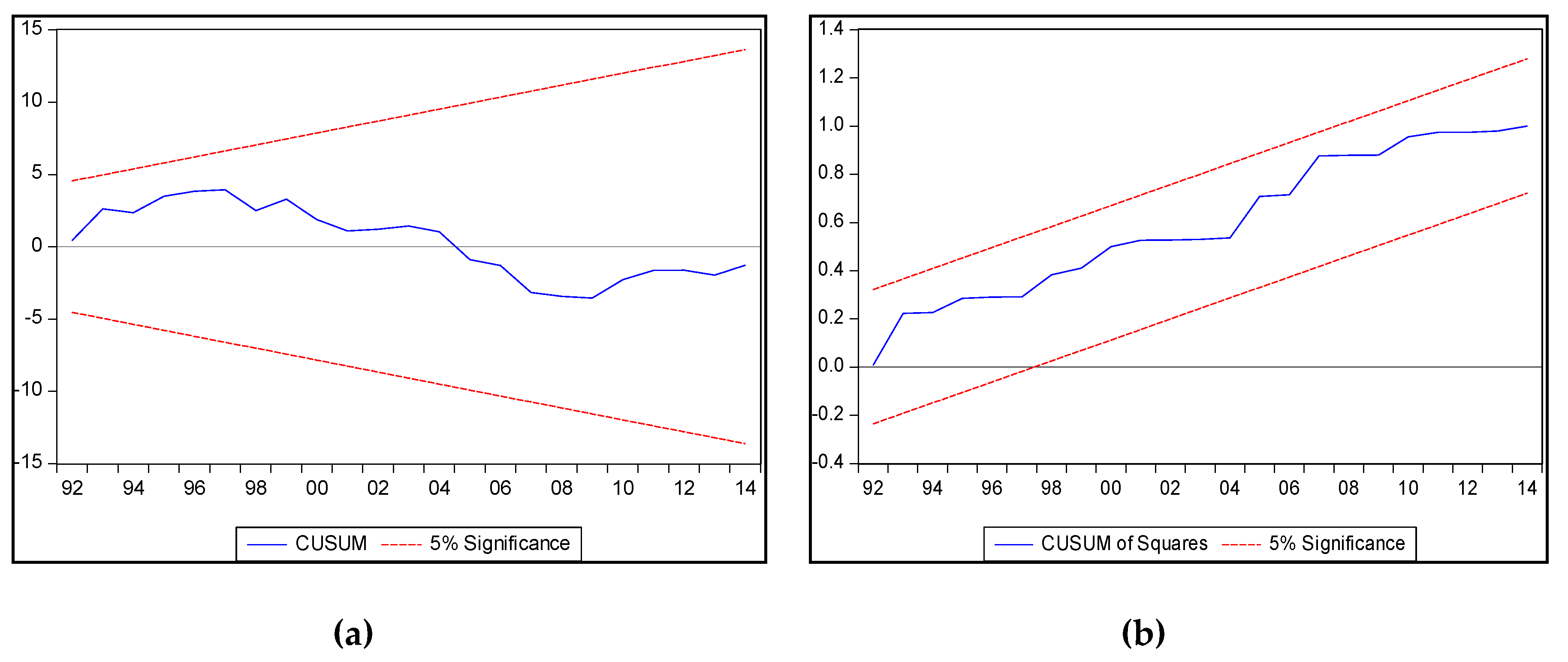
3.6. Model Stability
4. Discussion and Conclusions
Funding
Conflicts of Interest
Appendix A

| Countries | Periods | Methods | |
|---|---|---|---|
| Martinez-Zarzoso and Maruotti [12] | 88 developing countries | 1975–2003 | Stochastic Impacts by Regression on Population, Affluence and Technology (STIRPAT) model |
| Zhu et al. [13] | 20 emerging economies | 1992–2008 | semi-parametric panel data model |
| Sadorsky [14] | Emerging economies | 1971–2009 | STIRPAT model |
| Dogan and Turkekul [15] | USA | 1960–2010 | Autoregressive distributed lags (ARDL) |
| Ali et al. [16] | Singapore | 1970–2015 | Autoregressive distributed lags (ARDL) |
| He et al. [17] | China, regional | 1995–2013 | STIRPAT model |
| Bekhet and Othman [18] | Malaysia | 1971–2015 | VECM |
| Pata [19] | Turkey | 1974–2013 | Autoregressive distributed lags (ARDL) |
| Pata [20] | Turkey | 1974–2014 | Autoregressive distributed lags (ARDL), FMOLS |
| Countries | Periods | Methods | |
|---|---|---|---|
| Menyah and Wolde_Rufael [21] | US | 1960–2007 | Vector Auto regression |
| Apergis et al [22] | 19 developed and developing countries | 1984–2007 | Panel error correction model |
| Iwata et al. [23] | France | 1960–2003 | ARDL |
| Shafiel and Salim [24] | 29 OECD 1 countries | 1980–2011 | STIRPAT model |
| Jaforullah and King [25] | US | 1965–2012 | VECM |
| Bilgili et al [26] | 17 OECD countries | 1977–2010 | Panel FMOLS, Panel DOLS |
| Dogan and Seker [27] | European Union | 1980–2012 | Panel Dynamic Ordinary Least Squares |
| Ito [28] | 42 developing countries | 2002–2011 | GMM and PMG |
| Zoundi [29] | 25 selected African countries | 1980–2012 | Panel cointegration (Dynamic OLS, System GMM, etc.) |
References
- Intergovernmental Panel on Climate Change. Climate Change 2014: Impacts, Adaptation, and Vulnerability Part A: Global and Sectoral Aspects. In Working Group II Contribution to the Fifth Assessment Report of the Intergovernmental Panel on Climate Change, 1st ed.; Field, C.B., Barros, V.R., Eds.; Cambridge University Press: New York, NY, USA, 2014. [Google Scholar]
- Pao, H.T.; Tsai, C.M. Multivariate Granger causality between CO2 emissions, energy consumption, FDI (foreign direct investment) and GDP (gross domestic product): Evidence from a panel of BRIC (Brazil, Russian Federation, India, and China) countries. Energy 2011, 36, 685–693. [Google Scholar] [CrossRef]
- Seker, F.; Ertugrul, H.M.; Cetin, M. The impact of foreign direct investment on environmental quality: A bounds testing and causality analysis for Turkey. Renew. Sustain. Energy Rev. 2015, 52, 347–356. [Google Scholar] [CrossRef]
- Zhu, H.; Duan, L.; Guo, Y.; Yu, K. The effects of FDI, economic growth and energy consumption on carbon emissions in ASEAN-5: Evidence from panel quantile regression. Econ. Model. 2016, 58, 237–248. [Google Scholar] [CrossRef] [Green Version]
- Behera, S.R.; Dash, D.P. The effect of urbanization, energy consumption, and foreign direct investment on the carbon dioxide emission in the SSEA (South and Southeast Asian) region. Renew. Sustain. Energy Rev. 2017, 70, 96–106. [Google Scholar] [CrossRef]
- Tang, C.F.; Tan, B.W. The impact of energy consumption, income and foreign direct investment on carbon dioxide emissions in Vietnam. Energy 2015, 79, 447–454. [Google Scholar] [CrossRef]
- Mert, M.; Bolok, G. Do foreign direct investment and renewable energy consumption affect the CO2 emissions? New evidence from a panel ARDL approach to Kyoto Annex countries. Environ. Sci. Pollut. Res. 2016, 23, 21669–21681. [Google Scholar]
- Abdouli, M.; Hammami, S. Investigating the causality links between environmental quality foreign direct investment and economic growth in MENA countries. Int. Bus. Rev. 2017, 26, 264–278. [Google Scholar] [CrossRef]
- Merican, Y.; Yusop, Z.; Mohd Noor, Z.; Law, S.H. Foreign direct investment and the pollution in Five ASEAN Nations. Int. J. Econ. Manag. 2007, 1, 245–261. [Google Scholar]
- Peng, H.; Tan, X.; Li, Y.; Hu, L. Economic growth, foreign direct investment and CO2 emissions in China: A panel granger causality analysis. Sustainability 2016, 8, 233. [Google Scholar] [CrossRef] [Green Version]
- Zhang, C.; Zhou, X. Does foreign direct investment lead to lower CO2 emissions? Evidence from a regional analysis in China. Renew. Sustain. Energy Rev. 2016, 58, 943–951. [Google Scholar] [CrossRef]
- Martinez-Zarzoso, I.; Maruotti, A. The impact of urbanization on CO2 emissions: Evidence from developing countries. Ecol. Econ. 2011, 70, 1344–1353. [Google Scholar] [CrossRef] [Green Version]
- Zhu, H.-M.; You, W.-H.; Zeng, Z.F. Urbanization and CO2 emissions: A semi-parametric panel data analysis. Econ. Lett. 2012, 117, 848–850. [Google Scholar]
- Sadorsky, P. The effect of urbanization on CO2 emissions in emerging economies. Energy Econ. 2014, 41, 147–153. [Google Scholar] [CrossRef]
- Dogan, E.; Turkekul, B. CO2 emissions, real output, energy consumption, trade, urbanization and financial development: Testing the EKC hypothesis for the USA. Environ. Sci. Pollut. Res. 2016, 23, 1203–1213. [Google Scholar] [CrossRef]
- Ali, H.S.; Abdul-Rahim, A.S.; Ribadu, M.B. Urbanization and carbon dioxide emissions in Singapore: Evidence from ARDL approach. Environ. Sci. Pollut. Res. 2017, 24, 1967–1974. [Google Scholar] [CrossRef]
- He, Z.; Xu, S.; Shen, W.; Long, R.; Chen, H. Impact of urbanization on energy related CO2 emission at different development levels: Regional difference in China based on panel estimation. J. Clean. Prod. 2017, 140, 1719–1730. [Google Scholar] [CrossRef]
- Bekhet, H.A.; Othman, N.S. Impact of urbanization growth on Malaysia CO2 emissions: Evidence form the dynamic relationship. J. Clean. Prod. 2017, 154, 374–388. [Google Scholar] [CrossRef] [Green Version]
- Pata, U.K. The effect of urbanization and industrialization on carbon emissions in Turkey: Evidence form ARDL bounds testing procedure. Environ. Sci. Pollut. Res. 2018, 25, 7740–7747. [Google Scholar] [CrossRef]
- Pata, U.K. Renewable energy consumption, urbanization, financial development, income and CO2 emissions in Turkey: Testing EKC hypothesis with structural breaks. J. Clean. Prod. 2018, 187, 770–779. [Google Scholar] [CrossRef]
- Menyah, K.; Wolde-Rufael, Y. CO2 emissions, nuclear energy, renewable energy and economic growth in the US. Energy Policy 2010, 38, 2911–2915. [Google Scholar] [CrossRef]
- Apergis, N.; Payne, J.E.; Menyah, K.; Wolde-Rufael, Y. On the causal dynamics between emissions, nuclear energy, renewable energy, and economic growth. Ecol. Econ. 2010, 69, 2255–2260. [Google Scholar] [CrossRef]
- Iwata, H.; Okada, K.; Samreth, S. Empirical study on the environmental Kuznets curve for CO2 in France: The role of nuclear energy. Energy Policy 2010, 38, 4057–4063. [Google Scholar] [CrossRef] [Green Version]
- Shafiei, S.; Salim, R.A. Non-renewable and renewable energy consumption and CO2 emissions in OECD countries: A comparative analysis. Energy Policy 2014, 66, 547–556. [Google Scholar] [CrossRef] [Green Version]
- Jaforullah, M.; King, A. Does the use of renewable energy sources mitigate CO2 emissions? A reassessment of the US evidence. Energy Econ. 2015, 49, 711–717. [Google Scholar]
- Bilgili, F.; Koçak, E.; Bulut, Ü. The dynamic impact of renewable energy consumption on CO2 emissions: A Revisited Environmental Kuznets Curve approach. Renew. Sustain. Energy Rev. 2016, 54, 838–845. [Google Scholar] [CrossRef]
- Dogan, E.; Seker, F. Determinants of CO2 emissions in the European Union: The role of renewable and non-renewable energy. Renew. Energy 2016, 94, 429–439. [Google Scholar] [CrossRef]
- Ito, K. CO2 emissions, renewable and non-renewable energy consumption, and economic growth: Evidence from panel data for developing countries. Int. Econ. 2017, 151, 1–6. [Google Scholar] [CrossRef]
- Zoundi, Z. CO2 emissions, renewable energy and the Environmental Kuznets Curve, a panel cointegration approach. Renew. Sustain. Energy Rev. 2017, 72, 1067–1075. [Google Scholar] [CrossRef]
- Fernández, V.C.; Fernández, J.T. The long run impact of foreign direct investment, exports, imports and GDP: Evidence for Spain from an ARDL approach. EHES Work. Pap. 2018, 128, 1–21. [Google Scholar]
- Talukdar, D.; Meisner, C.M. Does the private sector help or hurt the environment? Evidence from carbon dioxide pollution in developing countries. World Dev. 2001, 29, 827–840. [Google Scholar]
- Pesaran, M.H.; Pesaran, B. Working with Microfit 4.0: Interactive Econometric Analysis; Oxford University Press: Oxford, UK, 1997. [Google Scholar]
- Pesaran, M.H.; Shin, Y. An autoregressive distributed lag modelling approach to cointegration analysis. In Econometrics and Economic Theory in the 20th Century: The Ranger Frisch Centennial Symposium; Strom, S., Holly, A., Diamond, P., Eds.; Cambridge University Press: Cambridge, UK, 1999. [Google Scholar]
- Pesaran, M.H.; Shin, Y.; Smith, R.J. Bounds testing approaches to the analysis of level relationships. J. Appl. Econom. 2001, 16, 289–326. [Google Scholar] [CrossRef]
- Engle, R.F.; Granger, C.W.J. Co-integration and Error Correction: Representation, Estimation, and Testing. Econometrica 1987, 55, 251–276. [Google Scholar] [CrossRef]
- Johansen, S.; Juselius, K. Maximum likelihood estimation and inference on cointegration with applications to the demand for money. Oxf. Bull. Econ. Stat. 1990, 52, 169–210. [Google Scholar] [CrossRef]
- Shrestha, M.B.; Bhatta, G.R. Selecting appropriate methodological framework for time series data analysis. J. Financ. Data Sci. 2018, 4, 71–89. [Google Scholar] [CrossRef]
- Harris, R.; Sollis, R. Applied Time Series Modeling and Forecasting; Wiley: Somerset, NJ, USA, 2003. [Google Scholar]
- World Bank DataBank. Available online: https://databank.worldbank.org/home.aspx (accessed on 1 September 2019).
- Korea Energy Statistical Information System. Available online: https://www.kesis.net/ (accessed on 1 September 2019).
- Narayan, P.K. The saving and investment nexus for China: Evidence from cointegration tests. Appl. Econ. 2005, 37, 1979–1990. [Google Scholar] [CrossRef]
- Brown, R.L.; Durbin, J.; Evans, J.M. Techniques for Testing the Constancy of Regression Relations over Time. J. R. Stat. Soc. 1975, 37, 149–163. [Google Scholar]


| Countries | Periods | Methods | |
|---|---|---|---|
| Pao and Tsai [2] | BRICs (Brazil, Russia, India, China) | 1992–2007 | Panel Vector Error Correction Model |
| Seker et al. [3] | Turkey | 1974–2010 | Autoregressive Distributive Lag (ARDL) |
| Zhu et al. [4] | ASEAN (South East Asian Nations) Countries | 1981–2011 | Fixed effect panel quantile regression |
| Behera and Dash [5] | SSEA (South and Southeast Asian), 17 countries | 1980–2012 | Panel Vector Error Correction Model) |
| Tang and Tan [6] | Vietnam | 1976–2009 | VECM (Vector Error Correction Model) |
| Mert and Bӧlӧk [7] | 21 Kyoto Annex I Countries | 1970–2010 | Panel Autoregressive Distributive Lag (ARDL) |
| Abdouli and Hammami [8] | MENA (Middle Eastern and North African), 17 countries | 1990–2012 | Panel VAR (Vector Auto regression) |
| Merican et al. [9] | Malaysia, Thailand, Indonesia, Singapore, Philippines | 1970–2001 | Autoregressive Distributive Lag (ARDL) |
| Peng et al. [10] | China, 16 provinces | 1985–2012 | Generalized Method of Moments (GMM) Panel granger Causality |
| Zhang and Zhou [11] | China, 11 eastern provinces, eight middle provinces, and 10 western provinces | 1995–2010 | Panel Vector Error Correction Model |
| Variables | ADF Test (at Level) | ADF Test (at First Difference) | PP Test (at Level) | PP Test (at First Difference) |
|---|---|---|---|---|
| −1.040 | −6.063 *** | −0.777 | −6.825 *** | |
| −0.994 | −5.683 *** | −0.976 | −13.968 *** | |
| −2.776 | −6.333 *** | −2.776 | −6.098 *** | |
| −2.750 | −4.496 *** | −2.766 | −4.620 *** | |
| −3.248 * | −0.931 | −3.254 * | −1.189 | |
| −2.585 | −4.165 ** | −1.876 | −4.029 ** |
| Selected Model: ARDL(2, 1, 0, 1, 0, 0) | ||||
| F-Bounds Test | ||||
| Test Statistic | Value | Significance | I(0) | I(1) |
| F-statistic | 4.299 | 10% | 1.81 | 2.93 |
| K = 5 | 5% | 2.14 | 3.34 | |
| 1% | 2.82 | 4.21 | ||
| t-Bounds Test | : = 0 | |||
| Test Statistic | Value | Significance. | I(0) | I(1) |
| t-statistic | −5.603 | 10% | −1.62 | −3.49 |
| 5% | −1.95 | −3.83 | ||
| 1% | −2.58 | −4.44 | ||
| Variable | Coefficient | Standard Error | t-Statistic | p-value |
|---|---|---|---|---|
| 0.776 *** | 0.061 | 12.683 | 0.000 | |
| −0.345 ** | 0.140 | −2.460 | 0.022 | |
| −0.405 *** | 0.104 | −3.902 | 0.001 | |
| 0.502 *** | 0.071 | 7.062 | 0.000 | |
| 0.055 ** | 0.021 | 2.666 | 0.014 | |
| Variable | Coefficient | Std. Error | t-Statistic | Probability | ||
|---|---|---|---|---|---|---|
| (−1) | 0.241 *** | 0.078 | 3.107 | 0.005 | ||
| 1.345 *** | 0.102 | 13.240 | 0.000 | |||
| −0.332 *** | 0.039 | −8.507 | 0.000 | |||
| ECT(−1) | −0.564 *** | 0.101 | −5.604 | 0.000 | ||
| R2 | 0.875 | Mean dependent variables | 0.036 | |||
| Adjusted R2 | 0.862 | Standard Deviation dependent variables | 0.056 | |||
| Standard error of regression | 0.021 | Akaike info criterion | −4.803 | |||
| Sum squared residuals | 0.012 | Schwarz criterion | −4.620 | |||
| Log likelihood | 80.848 | Hannan-Quinn criterion. | −4.742 | |||
| Durbin–Watson statistic | 2.118 | |||||
© 2020 by the author. Licensee MDPI, Basel, Switzerland. This article is an open access article distributed under the terms and conditions of the Creative Commons Attribution (CC BY) license (http://creativecommons.org/licenses/by/4.0/).
Share and Cite
Kim, S. The Effects of Foreign Direct Investment, Economic Growth, Industrial Structure, Renewable and Nuclear Energy, and Urbanization on Korean Greenhouse Gas Emissions. Sustainability 2020, 12, 1625. https://0-doi-org.brum.beds.ac.uk/10.3390/su12041625
Kim S. The Effects of Foreign Direct Investment, Economic Growth, Industrial Structure, Renewable and Nuclear Energy, and Urbanization on Korean Greenhouse Gas Emissions. Sustainability. 2020; 12(4):1625. https://0-doi-org.brum.beds.ac.uk/10.3390/su12041625
Chicago/Turabian StyleKim, Suyi. 2020. "The Effects of Foreign Direct Investment, Economic Growth, Industrial Structure, Renewable and Nuclear Energy, and Urbanization on Korean Greenhouse Gas Emissions" Sustainability 12, no. 4: 1625. https://0-doi-org.brum.beds.ac.uk/10.3390/su12041625