Comparison of HPLC Pigment Analysis and Microscopy in Phytoplankton Assessment in the Seomjin River Estuary, Korea

1
South Sea Research Institute, KIOST (Korea Institute of Ocean Science and Technology), Geoje 53201, Korea
2
K-water Institute, Korea Water Resources Corporation, Daejeon 34045, Korea
*
Author to whom correspondence should be addressed.
Sustainability 2020, 12(4), 1675; https://0-doi-org.brum.beds.ac.uk/10.3390/su12041675
Submission received: 30 January 2020
/
Revised: 18 February 2020
/
Accepted: 20 February 2020
/
Published: 24 February 2020
(This article belongs to the Special Issue Harmful Organisms and their Management for Sustainable Environment)
Abstract
:The distribution of microalgal species in estuaries shows marked gradients because of the mixing of marine and fresh water during tidal exchanges. To assess the spatio-temporal distribution of phytoplankton in the Seomjin River estuary (SRE), Korea, we investigated the seasonal phytoplankton communities along a salinity gradient in the estuary using both high performance liquid chromatography (HPLC) pigment analysis and light microscopy. Both types of analysis indicated that marine planktonic diatoms generally dominated at downstream sites having salinities >10, whereas freshwater species dominated at upstream sites having salinities <5. High levels of the pigments fucoxanthin and alloxanthin were found at upstream sites in the SRE in late spring. During summer, relatively high levels of the pigment peridinin were present in downstream areas of the SRE, and relatively high levels of diatoms occurred in upstream areas. In autumn, small Cryptomonas species were found in high abundance based on microscopic analysis, while CHEMTAX analysis of photosynthetic pigments showed relatively high concentrations of the diatom pigment fucoxanthin, implying the co-occurrence of a small unidentified phytoplankton. During winter, when the estuarine waters were well mixed, both the microscopic and CHEMTAX analyses showed that diatoms dominated at most stations. Seasonal and horizontal gradients in environmental conditions were clearly influenced by the salinity and nutrient loadings, especially the nitrate+nitrite and silicate concentrations. In particular, the ratio of photoprotective carotenoid pigments (PPCs) to photosynthetic carotenoid pigments (PSCs) was relatively low during all four seasons. This was predominately because of the high productivity of diatoms, which have a very low ratio of PPCs to PPSs. The SRE is a favorable habitat for diatoms because it is a high turbulence area having rapid water movement as a result of tidal changes. Overall, there was consistency in the data derived from the microscopy and chemotaxonomy analyses, suggesting that both methods are useful for analysis of the phytoplankton community structure in this complex estuarine and coastal water ecosystem.
1. Introduction
Estuaries are unique because they are environments where there are major changes in various gradients including temperature, salinity, nutrients, and turbulence [1]. They are also recognized as dynamic ecosystems where gradients in biological and chemical processes (e.g., algal biomass and nutrients) are associated with the mixing of freshwater and seawater during tidal changes [2]. As a result, estuaries support high biodiversity, which makes them suitable nursery grounds for a variety of macro-organisms, including valuable fish species [3]. Planktonic and benthic microalgal communities are key components in estuarine ecosystems, and their populations are controlled by environmental factors including salinity and nutrient gradients related to tidal water circulation [4]. However, although communities of small microalgae frequently dominate in estuaries, their populations have not been comprehensively quantified. It is important to accurately analyze the planktonic algal biomass and taxonomic groups in estuarine ecosystems, to enable evaluation of the biological dynamics of these systems. In addition, since estuaries are strongly influenced by human activities and have a direct impact on the ocean, many researches on aquatic environment have been conducted [5,6]. As the impact of climate change can be clearly identified, a lot of research has recently been conducted between climate change and aquatic ecosystem [7,8]. In particular, hydrological processes have been important global concerns for environmental sustainability due to enhanced climate variability such as extreme drought and flooding [9]. Subsequently, estuarine environments have been impacted by a changing hydrological cycle, and estuarine eco-hydrology has become one of the most important and essential research areas to understand the environmental sustainability of coastal waters.
Qualitative and quantitative analysis of microalgae using optical microscopy has been commonly used to assess biomass or biodiversity [10]. However, microscopic analysis is time consuming, and requires taxonomic experience to identify organisms to genus or species levels [11]. Moreover, pico- and nano-sized microalgae including green algae, cyanobacteria, and flagellates generally dominate in estuaries and freshwater, and it is very difficult to identify these using microscopy, often leading to errors or omissions in species identifications [12,13]. In contrast to microscopy for microalgal enumeration, photosynthetic pigments of pico- and nano-sized phytoplankton can be readily detected using HPLC, and this can provide data complementary to that from direct cell counts [14,15]. Photosynthetic biomarker pigments (e.g., fucoxanthin for diatoms, peridinin for dinoflagellates, alloxanthin for cryptophytes, zeaxanthin for cyanobacteria, chlorophyll b for chlorophytes, 19’-hex-fucoxanthin for haptophytes, and 19’but-fucoxanthin for pelagophytes) can be used in HPLC analysis, enabling rapid quantification of specific phytoplankton groups [12]. The analysis of photosynthetic marker pigments using the CHEMTAX program (CSIRO Marine Laboratories, Hobart, Tasmania, Australia) has been widely applied to the quantification of phytoplankton communities and biomass in coastal waters and estuaries [14,16], and in freshwater [17].
The HPLC-CHEMTAX tool was useful for identifying seasonal patterns in offshore and coastal waters and salinity gradients in estuaries, and was also able to distinguish estuary systems based on the phytoplankton community structure [18]. Phytoplankton indicators based on these pigments have been proposed in sustainable water quality and eutrophication assessment in international policies [19,20]. Roy et al. [21] and Chai et al. [22] reported that photosynthetic marker pigments can be used as indicators of trophic physiological conditions for phytoplankton communities, which can be affected by environmental conditions and trophic status in southwest coast of India and the Pearl River estuary, respectively. Gibb et al. [23] and Barlow et al. [15] reported that PPCs dominate in low productivity waters, whereas PSCs dominate in high productivity waters in the Atlantic Ocean. This suggests that the ratio of PPCs to PSCs can be used as an indicator of the environmental status and tropic levels in relation to biological and chemical gradients in dynamic estuarine ecosystems. Increased irradiance and reduced nutrients significantly increase the proportion of photoprotective carotenoids and consequently increase the ratio of PPCs to PSCs [15]. Moreno et al. [24] also reported that PPCs are greatly influenced by high irradiance levels on the Argentinian continental shelf, suggesting that this parameter may respond to environmental changes. Thus, the PPCs to PSCs ratio may be useful in assessing the water column environmental factors related to phytoplankton growth, including cellular responses. Therefore, these tools can be used to assess ecological characteristics for a sustainable environment related with the possibility of identifying the diversity of functional groups and their reaction to various environmental conditions.
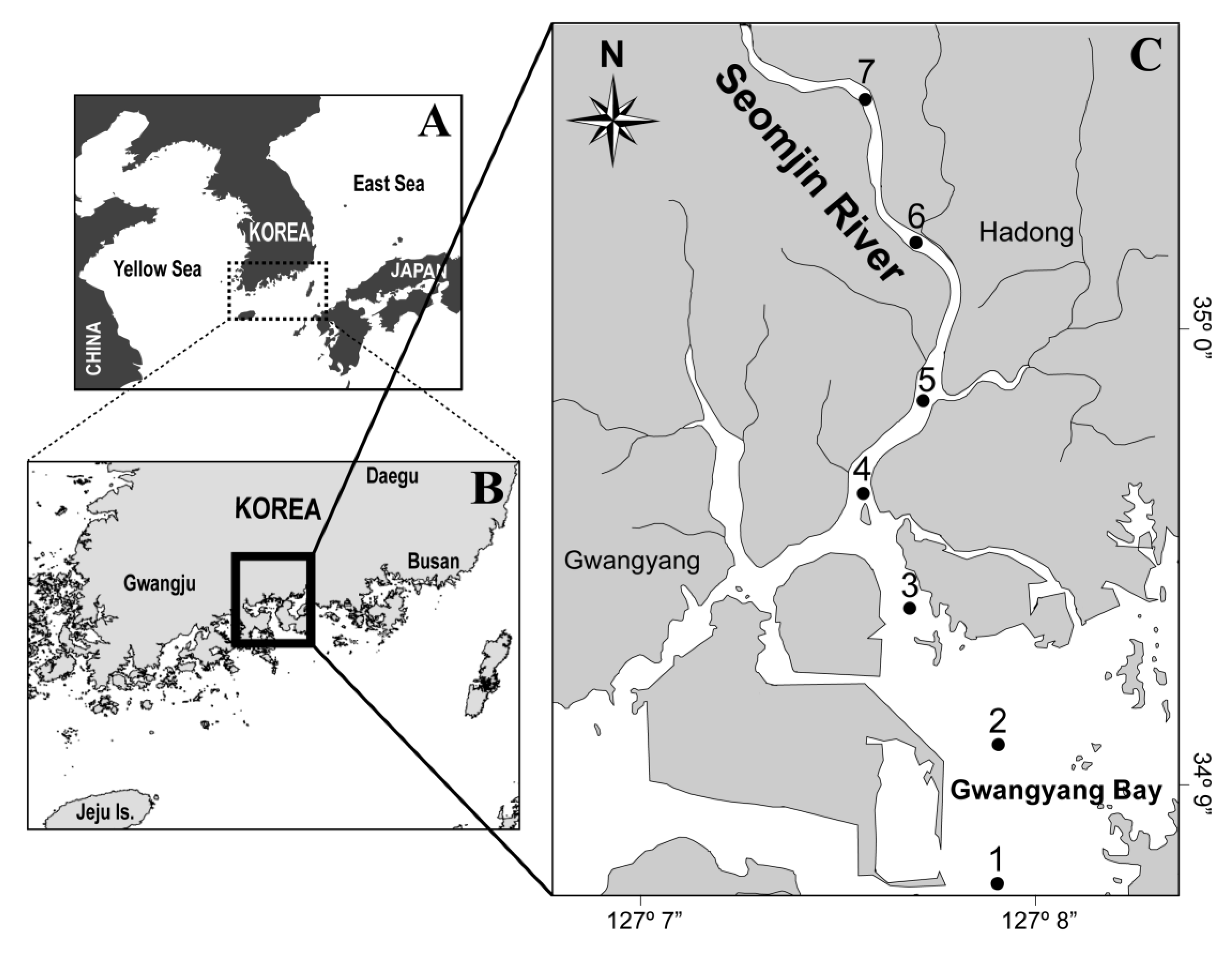
The Seomjin River is the fifth largest river in Korea, and the SRE is located in the southern part of Korea. The Seomjin River has a watershed area of 4900 km2, and it flows into the northern part of Gwangyang Bay, which is connected to the offshore waters of the Southern Sea of Korea [25]. The Seomjin River has a relatively small inflow of pollutants from upstream, except pollutants from Gwangyang Bay. Gwangyang Bay is a shallow inner bay that is subject to a variety of anthropogenic impacts, including steel manufacturing, petrochemical industry complexes, the transit of cargo vessels, and a harbor [26]. In addition, the SRE is also an important habitat for the brackish water clam Corbicula japonica, an economically valuable fishery resource for the local community in Korea [26]. Therefore, ecological and environmental assessment of environmental change in the SRE is very important, but there have been few studies evaluating biodiversity in communities of small phytoplankton in relation to salinity gradients, although several studies have focused on hydrological processes [27] and pollution [28]. Therefore, analysis of changes in phytoplankton community biodiversity is essential to enable assessment of species composition and the trophic status of estuarine ecosystems. In this study, we analyzed the spatial and temporal distribution of members of the phytoplankton community using both microscopic observations and HPLC analysis of cellular marker pigments. In addition, we evaluated the functional community structure based on analysis of PPCs and PSCs in relation to environmental factors in the SRE. These are expected to give more insights to understand the estuarine ecological features for sustainable eco-hydrological processes.
2. Materials and Methods
2.1. Field Sampling
Water samples were collected during spring tides at seven stations (Figure 1) on flood tides. The sampling stations were located throughout the SRE, with Station 1 being the most downstream and Station 7 the most upstream. Seasonal sampling was conducted in late spring (18 June 2015), summer (12 August 2015), autumn (10 November 2015), and winter (20 February 2016). Although one-time surveys cannot represent all weather conditions, the surveys were conducted by selecting a period that was the most representative of each season. Since this area is affected by monsoons, it heats up after the rainy season starting in late June or July, so the survey was carried out in late spring. Summer surveys were conducted at the highest temperatures after the rainy season. Autumn and winter surveys were also conducted during times when there were no events such as heavy rainfall and typhoons. On each occasion the sampling was completed within 2 h to minimize the influence of tidal range on the water flow. Horizontal profiles of temperature, salinity, and the dissolved oxygen (DO) concentration were measured concurrently using a conductivity–temperature–depth (CTD) sensor and a YSI data sonde (CTD: Ocean Seven 319; Idronaut Co., Brugherio, Italy; YSI: YSI data sonde; USA). We collected surface water using a bucket. The water samples for nutrient analysis were filtered (GF/F; 47 mm; Whatman, Middlesex, UK), placed in acid-cleaned polyethylene bottles, and fixed using HgCl2. For pigments, we collected replicate samples at each station. Each sample was filtered through a 47-mm diameter GF/F filter (Whatman, Middlesex, UK) using 1L of the water sample, and the filter was stored at −20 °C until further laboratory analysis. To identify and enumerate phytoplankton using microscopy, 0.5 L subsamples were stored in polyethylene bottles and fixed with 2% (final concentration) Lugol’s solution. For measurement of nutrient concentrations, each filtered water sample was stored at −20 °C.
2.2. Nutrients Analysis
The concentrations of nutrients in the filtered water samples, including ammonia, nitrate, nitrite, phosphate, and silicate, were determined using a flow injection auto-analyzer (QuikChem 8000; Lachat Instruments, Loveland, CO, USA). The nutrient concentrations were calibrated using standard brine solutions (CSK Standard Solutions; Wako Pure Chemical Industries, Osaka, Japan).
2.3. Phytoplankton Identification Using Microscopy
Subsamples for phytoplankton identification were concentrated to approximately 50 mL by decanting the supernatant. The concentrated subsamples were loaded onto a Sedgewick-Rafter counting chamber after gentle mixing, and phytoplankton were counted using an optical microscope (Carl Zeiss; 37081 Gottingen, Germany) at 200× magnification. The identification of phytoplankton was performed using optical microscopy at 400× magnification. The dominant diatom and dinoflagellate members of the communities were identified to species level. In addition, to enable comparison with pigment analyses based on HPLC and the CHEMTAX program, the nanophytoplankton species were identified to class level.
2.4. HPLC Analysis
Photosynthetic marker pigments including chl-a were analyzed as described by Zapata et al. [29] using HPLC (LC-10A system; Shimadzu Co., Kyoto, Japan) with a Waters C8 column (150 × 4.6 mm, 3.5 μm particle size, 0.01 μm pore size; Waters Corporation, Milford, MA, USA) for separation. The pigments were extracted using 95% methanol (5 mL) at 4 °C for 24 h in darkness. Following extraction each sample was sonicated and centrifuged, and 1 mL of the supernatant was mixed with 0.3 mL of deionized water prior to injection into the HPLC column. The standard pigments were used to identify the pigment peaks, and to calibrate the pigment concentrations on the basis of the peak areas. The pure standard pigments were obtained from Sigma Chemical and DHI (Hørsholm, Denmark), as shown in Table 1.
2.5. CHEMTAX Program
On the basis of the measured pigment concentrations, the phytoplankton community composition was estimated using the CHEMTAX program, as described by Mackey et al. [30]. CHEMTAX is statistical software used to estimate the biomass of various phytoplankton functional groups based on calculation of the ratio of marker pigments to that of chl-a [30,31]. In the MATLAB (The Mathworks, Inc.) programming environment, CHEMTAX uses factor analysis and a descent algorithm to determine the phytoplankton class proportions fitted to the total pigment concentrations, based on a cellular pigment ratio for each algal group. The diagnostic biomarker pigments used included chl-a, fucoxanthin, 19′-hexanoyloxy-fucoxanthin, 19′-butanoyloxy-fucoxanthin, peridinin, prasinoxanthin, lutein, alloxanthin, zeaxanthin, violaxanthin, neoxanthin, and chlorophyll-b. The initial ratios of the marker pigments to chl-a for chlorophytes, dinoflagellates, diatoms, and cyanobacteria were estimated based on the results of Mackey et al. [30], as shown in Table 2.
2.6. Pigment Indices
2.7. Environmental Data and Statistical Analysis
Water fluxes and river discharges were based on serially complete daily runoff data provided by the Korean Water Resources Management Information System (WAMIS; http://www.wamis.go.kr/eng/main.aspx), and daily precipitation data were provided by the Korea Meteorological Administration (KMA; http://www.kma.go.kr/eng/weather/climate/worldclimate.jsp). The relationship between the measured environmental factors (temperature, salinity, DO, phosphate, ammonium; NOx: nitrate + nitrite; and silicate) and the occurrence of dominant phytoplankton species was investigated using canonical correspondence analysis (CCA), using CANOCO for Windows 4.5 (Biometris, Wageningen, The Netherlands). The CCA enabled exploration of the relationships of the community to environmental factors [32]. All statistical calculations were performed using the XLSTAT 2010 (Addinsoft Inc., Brooklyn, NY, USA) program and SPSS version 17.0 (SPSS Inc., Chicago, IL, USA).
3. Results
3.1. Environmental Factors
The levels of environmental factors including precipitation, runoff, water temperature, and nutrients in the SRE from 2015 to 2016 are shown in Table 3.
There was no eventual precipitation and water discharge because surveys were conducted when it was not affected by intensive rainfall or typhoon, and they tended to increase slightly toward autumn. The water temperature ranged from 6.4 °C to 26.9 °C and was lowest in winter and highest in summer. The water temperature at the upstream stations was generally higher than at the downstream stations in the SRE during summer, whereas the upstream stations had lower water temperatures than the downstream stations in winter. The mixing of freshwater and seawater in the SRE led to changes in salinity (9.8–33.1), and marked differences between the upstream and downstream stations were found. There was large spatial variation in nutrient concentrations between upstream areas of the SRE and the inner area of Gwangyang Bay (Figure 1). NOx ranged from 1.0 μm to 58.5 μm, and was strongly dependent on freshwater input, particularly at upstream stations (Station 7). Although the spatial distribution of ammonium in the SRE was not clear, the highest seasonal ammonium concentrations were observed in the middle of the estuary, where there is a fishery port and associated town. The ammonium concentration in the SRE varied from 0.4 μm to 7.4 μm, with levels being particularly high in autumn and low in winter. The phosphate concentration ranged from 0.23 μm to 1.10 μm, and varied little compared with the concentrations of N and Si. The silicate concentration ranged from 8.17 μm to 74.19 μm, and remained relatively high in the SRE, particularly in the upstream areas.
3.2. Distribution of Pigments and Phytoplankton Biomass
Figure 2 and Table 4 shows the spatial and temporal variations in the chl-a concentration and phytoplankton abundance. The chl-a concentration was low in autumn and winter but was relatively high in spring and summer. The trends in chl-a concentration and abundance of phytoplankton were similar, even though the spatio-temporal distribution patterns differed slightly. In particular, the chl-a concentration and phytoplankton abundance increased toward the upper SRE in spring, summer, and autumn, whereas the biomass in winter was high at Station 1 in the downstream area.
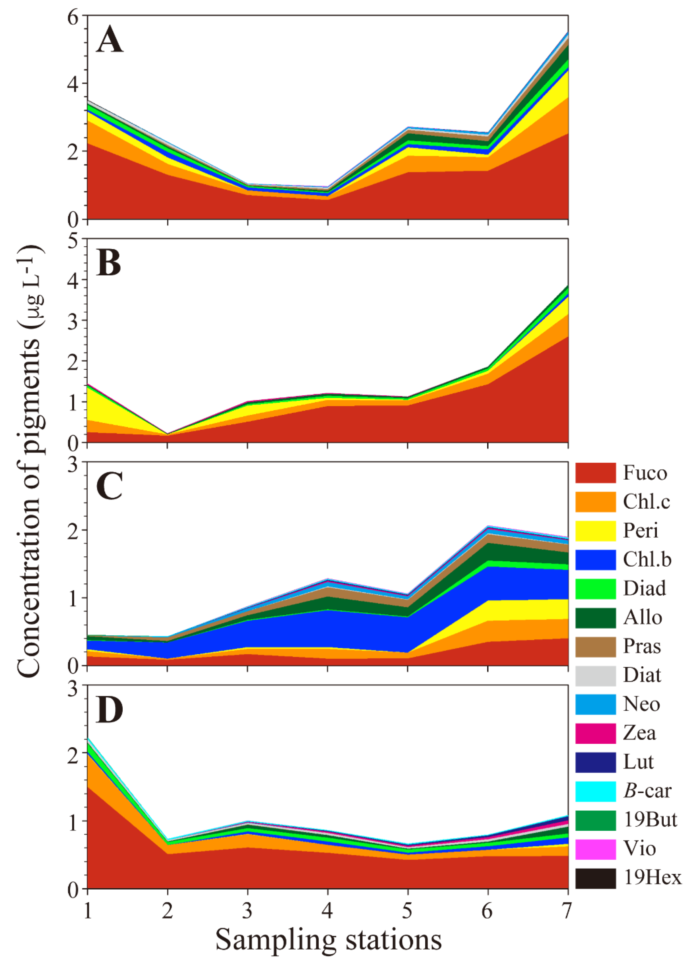
A total of 15 pigments were identified and their distributional characteristics are shown in Figure 3. In spring the fucoxanthin concentration ranged from 0.70 μg L−1 to 2.52 μg L−1, and remained relatively high, and reached 2.23 μg L−1 in the upstream area and 2.52 μg L−1 in the downstream area. In addition, the concentration of chl-c2, which is an accessory pigment in diatoms and showed a similar trend to the temporal distribution of fucoxanthin. The concentrations of diadinoxanthin and diatoxanthin ranged from 0.03 μg L−1 to 0.23 μg L−1 and 0.01 μg L−1 to 0.11 μg L−1, respectively. The concentrations of marker pigments for diatoms were high in both upstream and downstream areas, indicating that diatoms dominated during spring in the SRE. The concentration of peridinin, which is a marker pigment for dinoflagellates, was particularly high at stations 1 and 7. However, its concentration remained relatively low throughout the year. The total concentration of neoxanthin was low (0−0.08 μg L−1), and for prasinoxanthin varied from 0 μg L−1 to 0.20 μg L−1. The concentration of prasinoxanthin gradually increased from the downstream to the upstream areas. The concentration of alloxanthin, which is a marker pigment for cryptophytes, and remained particularly high in the upstream area. Chl-b was usually detected at most stations, and its concentration ranged from 0.06 μg L−1 to 0.16 μg L−1. In the downstream area, 19-hexcanoyloxyfucoxanthin was detected at station 1. Minor pigments including violaxanthin, zeaxanthin, and lutein were also detected in upstream areas, particularly at stations 5 and 7, but their concentrations did not exceed 0.02 μg L−1.
In summer the fucoxanthin concentration varied from 0.16 to 2.60 μg L−1, and remained at high levels in the upstream area; this trend was opposite to that for the fucoxanthin concentration in spring. The chl-c2 concentration ranged from 0.03 to 0.55 μg L−1, and tended to be higher in upstream areas. The peridinin concentration ranged from 0 to 0.79 μg L−1, and it was remarkably high at station 1. The diadinoxanthin, alloxanthin, and zeaxanthin concentration were <0.14 μg L−1 in all station, and the concentration of chl-b was 0.08 μg L−1 at station 7.
Compared with other seasons, the pigment composition was markedly different in autumn. The chl-b concentration ranged from 0.13 to 0.54 μg L−1, and chl. b concentration was positively correlated with total biomass. In addition, the fucoxanthin concentration varied from 0.09 to 0.35 μg L−1, and the chl-c2 concentration ranged from 0.02 to 0.31 μg L−1. The alloxanthin concentration ranged from 0.0 to 0.26 μg L−1. The neoxanthin, prasinoxanthin, zeaxanthin, and β-carotene concentrations were <0.14 μg L−1 in the SRE.
In winter the pigment composition was relatively simple compared with the other seasons. Fucoxanthin mostly dominated, with concentrations ranging from 0.60 to 0.42 μg L−1. The highest measured chl-c2 concentration was 0.47 μg L−1 at Station 1, and the chl-c2 concentration ranged from 0.08 to 0.19 μg L−1 in the upstream area. The peridinin, alloxanthin, diatoxanthin, zeaxanthin, lutein, and chl-b concentrations remained <0.09 μg L−1.
3.3. Phytoplankton Abundance and Composition Based on Microscopy and Pigment Analysis
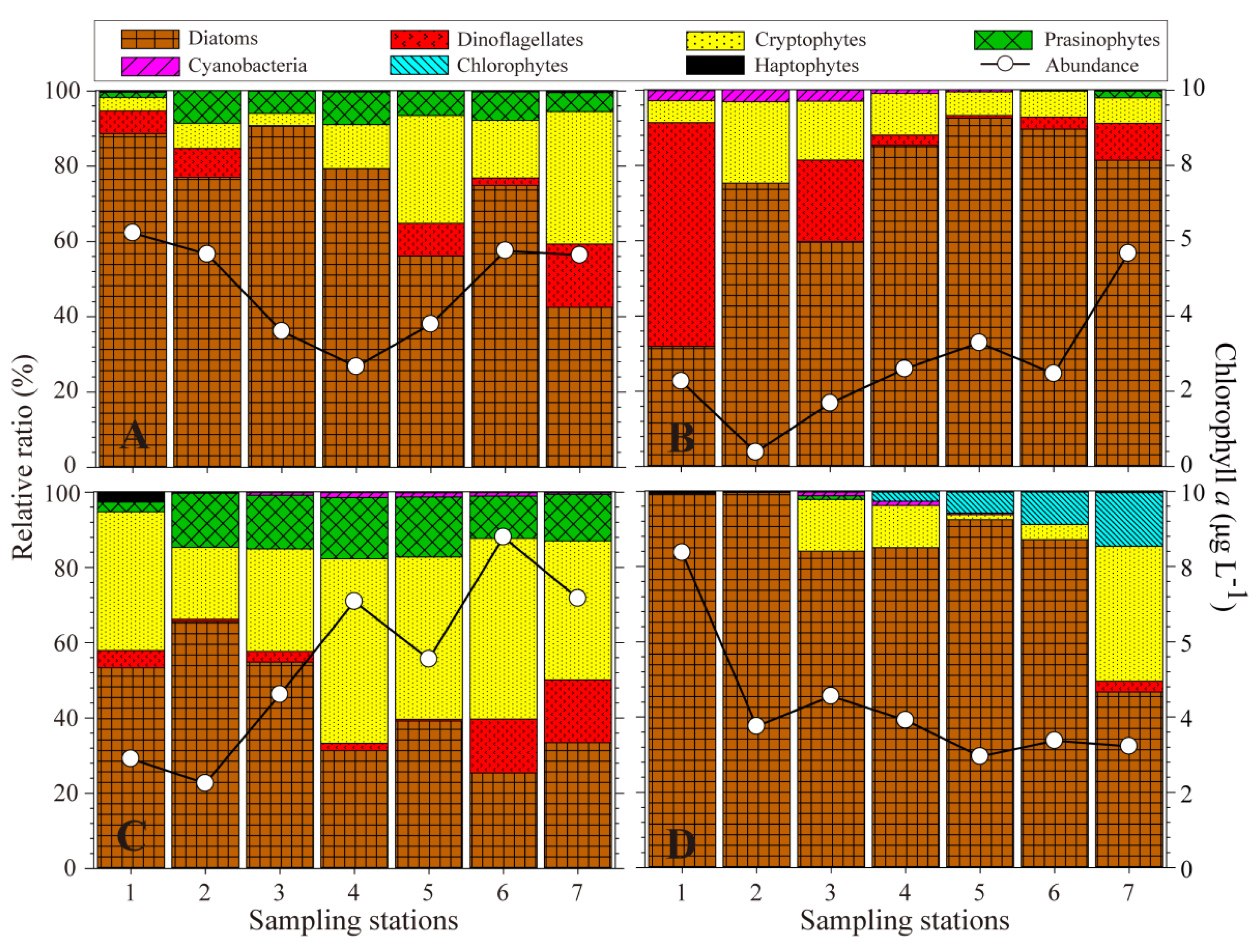
The CHEMTAX analysis indicated that in spring diatoms comprised 88.7% of the phytoplankton community at station 1 (downstream) but decreased toward the upstream areas (Figure 2). Cryptophytes increased in abundance from the downstream areas toward the upstream and comprised 35.2% of the community at station 7. The pigment-based abundance of diatoms and cryptophytes was consistent with the results of the microscopy analysis (Table 4), which showed that the diatoms mainly comprised Chaetoceros spp. (C. debilis, C. lorenzianus and C. socialis), Skeletonema spp., and Thalassionema frauenfeldii (Table 5).
The proportion of dinoflagellates at stations 1 and 2 was relatively high, and predominantly comprised Heterocapsa spp. and Prorocentrum spp. The CHEMTAX analysis indicated that in summer dinoflagellates comprised 59.5% of the community at station 1, but microscopic observations indicated they comprised 34.0%, particularly Cochlodinium polykrikoides. Diatoms dominated upstream areas (95.5% of the community). The main diatom species were Chaetoceros spp. and Skeletonema spp. in seawater regions (Stns. 1–5), but Aulacoseira spp. dominated in the freshwater region (station 7), reaching a maximum abundance of 2.82 × 10⁵ cells L−1. In autumn, diatoms and cryptophytes comprised 43.3% and 37.2% of the community, respectively, with the diatom abundance being relatively high in the downstream area, while cryptophytes dominated in the upstream area. Based on microscopic observations, the mean cryptophyte abundance was 2.2 × 10⁵ cells L−1 in the SRE area (92.5% of the community), indicating a discrepancy between the CHEMTAX and microscopy results. In winter, pigment analysis indicated diatoms comprised 84.9% of the community, which was a finding similar to that based on microscopic observations. Microscopy indicated high densities of Chaetoceros spp. at station 1, and high numbers of Thalassiosira pacifica and T. rotula were present in the SRE area.
4. Discussion
4.1. Comparison of Pigment and Microscopy Analyses in the SRE
It is known that microscopic analysis is not particularly useful for the identification of pico- and nano-sized phytoplankton. Pigment chemotaxonomy using CHEMTAX is considered an important technological tool for investigating phytoplankton community structure, particularly for identifying small estuarine microalgal species [33]. While microscopic observations can provide important taxonomic information for micro-sized species (>20 μm), identification is often difficult because of problems including cell shrinkage and lysis following fixation using Lugol’s solution, particularly for flagellated species. Andersen et al. [34] used scanning electron microscopy to aid identification of some eukaryotic microalgal species in oligotrophic open ocean waters, but this approach has limitations in estimating phytoplankton biomass. Recently, molecular tools including the real-time quantitative polymerase chain reaction have been applied to the identification and quantification of specific species. In addition, next generation sequencing (NGS) has been developed for the identification of multi-community levels of eukaryotic microalgal species. Although both these molecular tools provide very advanced techniques for detecting eukaryotic microalgal species, their application and maintenance is time consuming and expensive. In contrast, Suzuki et al. [35] and Andersen et al. [34] showed that pigment chemotaxonomy is useful for the identification and quantification of nano- and pico-phytoplankton that are difficult to analyze using optical microscopy for oligotrophic water of Pacific and Atlantic Oceans and Bering Sea. In addition to chemotaxonomy based on marker pigments, the CHEMTAX program has been used to estimate the contribution of each phytoplankton class to the total phytoplankton biomass [30] and is considered to be useful in the rapid and accurate analysis of photosynthetic pigments. Therefore, a comparison of pigment and microscopy analyses in assessment of phytoplankton biodiversity and biomass could provide useful information for investigating estuarine phytoplankton dynamics in relation to salinity and nutrient gradients, particularly for pigment-based chemotaxonomy of small estuarine microalga species.
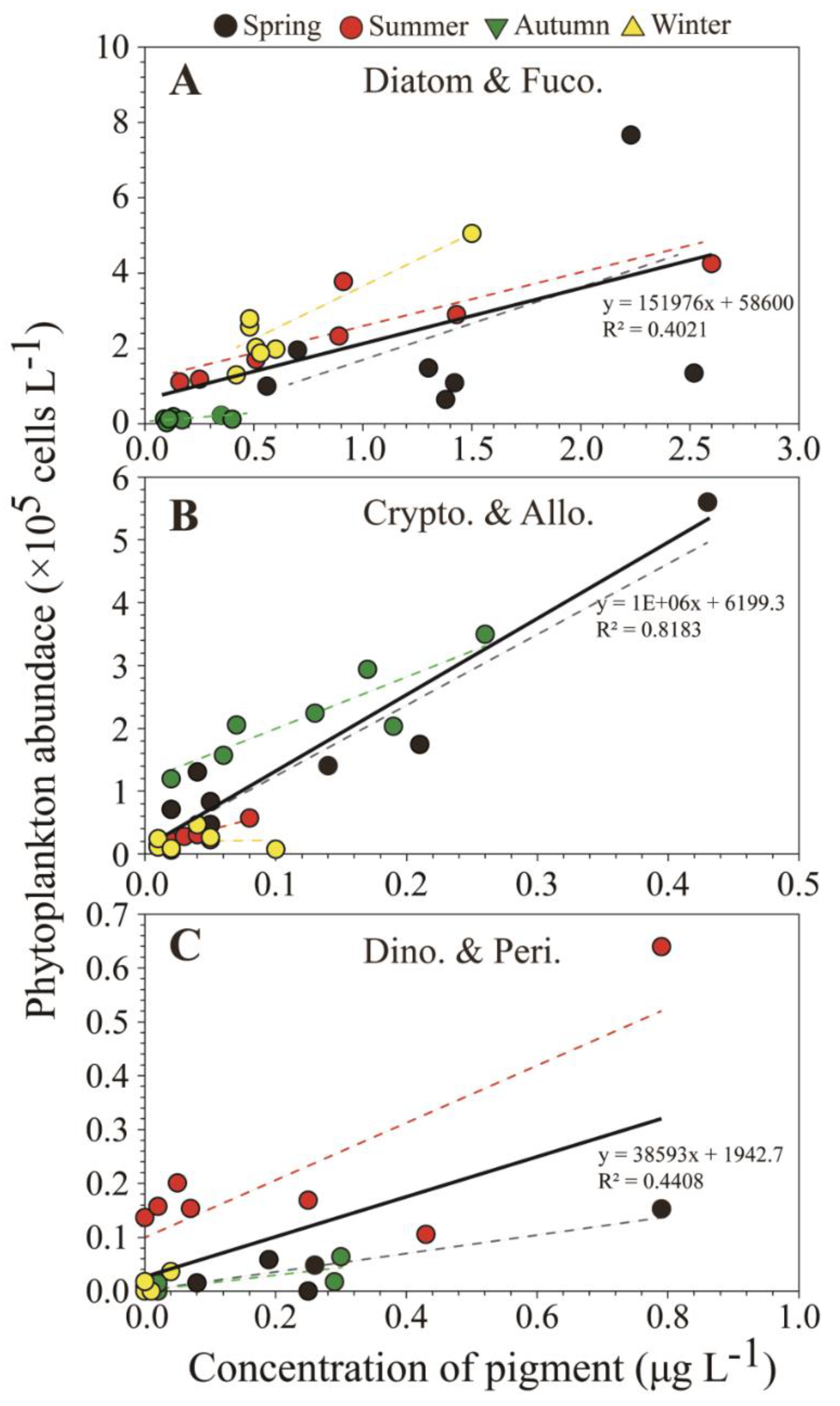
Prior to undertaking the comparison using CHEMTAX, we assessed statistical correlations for the SRE between HPLC-based pigment data and microscopy-based phytoplankton abundance. Silva et al. [36] demonstrated that statistical correlations between pigments and the abundance of each group is useful in determining phytoplankton composition, particularly for small phytoplankton groups in coastal and estuarine ecosystems. In the present study the seasonal concentrations of the carotenoid fucoxanthin was significantly correlated with diatoms abundances in the SRE (R2 = 0.40, p < 0.01; Figure 4A). There was a significant correlation between the concentration of this pigment and total diatom abundances in summer and winter, which corresponded to periods of high phytoplankton biomass in the SRE. The alloxanthin concentration showed a significant correlation (particularly in spring and autumn) with the abundance of cryptophytes including small Cryptomonas spp. (R2 = 0.82, p < 0.01; Figure 4B), implying that Cryptophyta are dominant in the SRE. In addition to these pigments, the seasonal concentration of peridinin was correlated with dinoflagellate abundances (R2 = 0.44, p < 0.01; Figure 4C), even though the peridinin concentration was usually relatively low in the SRE. However, the peridinin concentration at station 1 (downstream area) was relatively high in summer, corresponding to high abundances of the harmful red tide dinoflagellate Cochlodinium polykrikoides, and was relatively high in the downstream area in spring, coinciding with high abundances of Heterocapsa spp. and Prorocentrum spp. However, no microscopic evidence of dinoflagellates was found associated with the low peridinin concentrations detection in the upstream freshwater area in spring, summer, and autumn, indicating that microscopic analysis may not have identified the dinoflagellates from which the peridinin originated, perhaps because of cell lysis in the lower salinity water. Brewin et al. [37] and Rodriguez et al. [38] reported that HPLC pigment analysis does not completely reflect the phytoplankton community composition, but can provide more detailed information on the phytoplankton community structure than that obtained from direct optical microscopy observations alone. We hypothesized that a significant correlation between HPLC pigment concentrations and microscopic cell counts may enable more accurate assessment of total algal biomass through inclusion of damaged cells and unidentified small autotrophic organisms, which contribute to the spatio-temporal distribution of phytoplankton (diatoms, dinoflagellates, and unidentified flagellates) in the SRE.
In addition to correlations between pigment analysis and direct microscopy, phytoplankton classification using CHEMTAX can provide qualitative and quantitative data on the composition of phytoplankton, particularly in complex estuarine ecosystems. Gameiro et al. [39] reported that biomarker pigment concentration analysis using HPLC and CHEMTAX enabled identification of diatoms, dinoflagellates, cryptophytes, chlorophytes, euglenophytes, prasinophytes, cyanobacteria, and haptophytes in the Tagus River estuary, Portugal, and highlighted the reliability of HPLC-derived pigment analysis as a tool for the assessment of phytoplankton variability related to community diversity. In the present study, cyanobacteria (in summer) and chlorophytes (in winter) were not detected using optical microscopy, but were readily detected by CHEMTAX. In addition, prasinophytes (identified by the presence of prasinoxanthin) were detected in spring and autumn in the SRE (excluding station 1). Prasinophytes cannot be easily identified using optical microscopy because they are nano-sized and lack morphological distinguishing characteristics. Although the phytoplankton community structures in spring, summer, and winter based on microscopy and CHEMTAX were relatively consistent, the analyses differed in autumn. Based on microscopic observations the dominant group (95%) was Cryptomonas, whereas in the CHEMTAX analysis this group comprised 50% of the total phytoplankton community. The difference was related to the occurrence of large numbers of small cryptomonads. In contrast, the CHEMTAX analysis indicated a greater diatom abundance compared with direct observations, implying that relatively large diatom species have contributed to cellular pigment content in the SRE. Olenina [40] reported that the large size variation of cryptophytes (10–50 μm) results in a volume difference of approximately 10-fold. The relative ratios of photosynthetic pigments may have been greatly influenced by environmental conditions including nutrients and light intensity [30,41]; consequently, it is necessary to consider phytoplankton dynamics in relation to hydrological characteristics (see below).
In addition, it is very important to know not only species composition but also biomass and carbon for ecosystem analysis [42]. Although biomass is mainly calculated by microscopic analysis, it can also be sufficiently represented as chl-a, which is easy to analyze [43,44]. In addition, clear correlations have been reported between biomass and accessory pigments, and it can be used to determine which phytoplankton group contributes to the total biomass [45,46]. As a result, comparison of the two identification methods suggests that they can both contribute to understanding of the spatio-temporal changes in phytoplankton composition in complex estuarine ecosystems. Thus, it is considered as a good alternative method because the ecological analysis such as food web studies and carbon transfer using the marker pigment can clearly identify the group of phytoplankton contributing to the total biomass than the microscopic analysis.
4.2. Phytoplankton Population Dynamics in the SRE
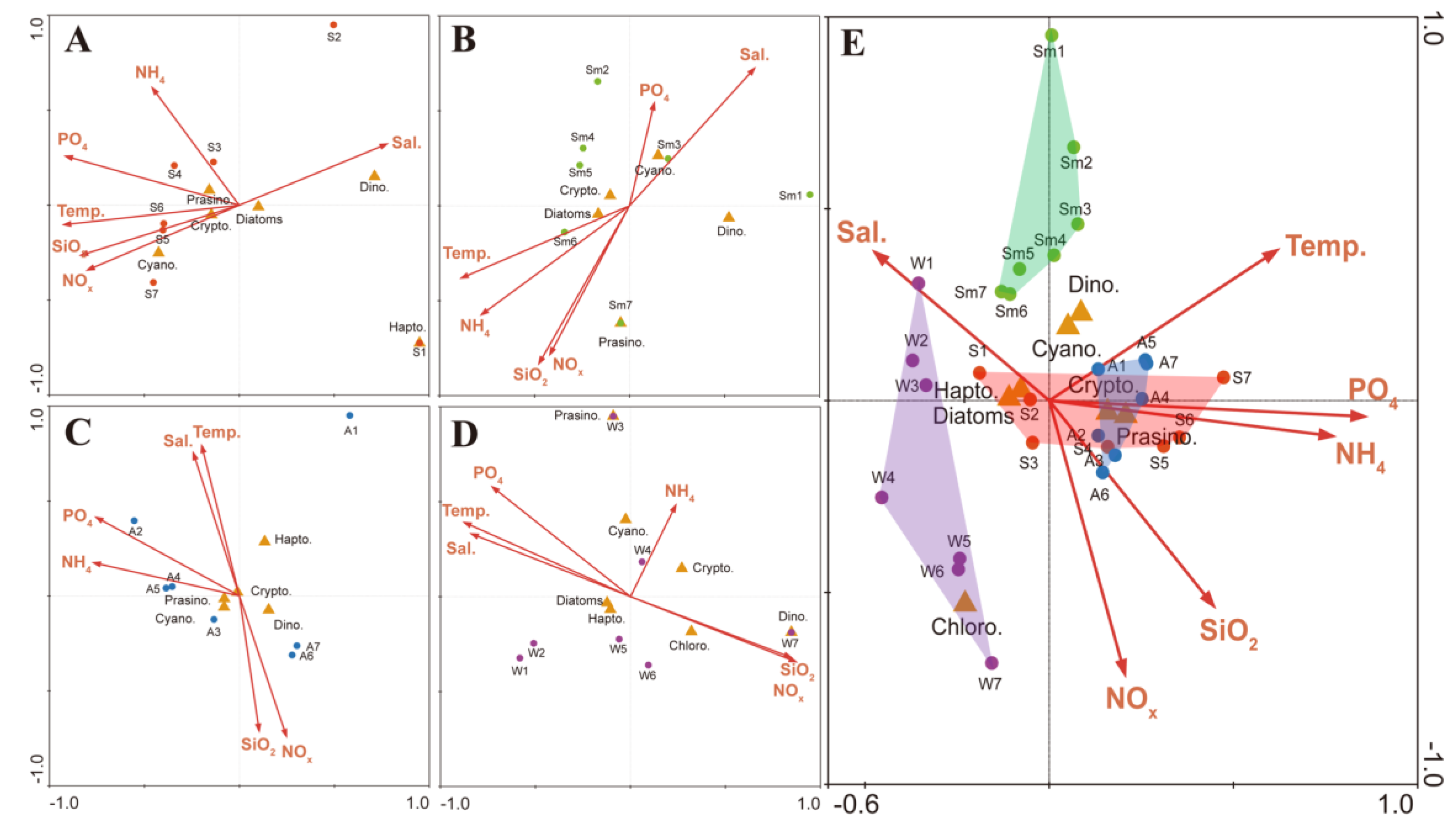
Both methods (microscopy and the pigment fucoxanthin) indicated that diatoms were dominant in spring. There was high relative abundance of the marine diatoms Chaetoceros, Skeletonema, and Thalassionema in the saltwater area, with T. frauenfeldii being the most dominant species. Thalassionema is a dominant species in the coastal waters of Korea, particularly in Gwangyang Bay [47]. The CCA analysis clearly showed that the horizontal distributions of diatom, dinoflagellates, and cryptophyte communities in the SRE were influenced by the salinity gradient, which was directly related to the nitrate+nitrite loadings, because of the negative correlation between salinity and nitrate+nitrite (Figure 5A). The silicate concentration and temperature were also correlated with the nitrate+nitrite concentration, but there was no significant relationship between salinity and the ammonium concentration, implying that nitrate+nitrite and silicate loadings resulted mainly from freshwater input from the Seomjin River. However, the concentrations of ammonium were relatively higher at downstream and midstream areas. Cryptophyte species (Cryptomonas spp.) were dominant at upstream sites (stations 5–7), and were correlated with the nitrate+nitrite and silicate loadings. In our previous study [47], cryptophytes were also dominant in estuarine areas. Thus, the horizontal distribution of the phytoplankton community in spring was influenced by the salinity gradient, with the implication that there was a direct response of phytoplankton to nutrient loading associated with the salinity gradient.
In summer, the peridinin concentration (dinoflagellate marker) was relatively high at station 1, which reflected the occurrence of dinoflagellates found in the CHEMTAX analysis, and the high abundances of the mixotrophic dinoflagellate C. polykrikoides based on optical microscopy; a large bloom of C. polykrikoides was reported in water offshore of Gwangyang Bay. Blooms of C. polykrikoides cause huge economic losses to fishery industries because of the mass mortality of caged fish, and these blooms occur annually in Korean coastal waters [48,49]. In the present study the high density of C. polykrikoides corresponded to high chl-a and peridinin concentrations, implying that C. polykrikoides accounted for most of the measured peridinin in downstream areas, even though there was a relatively high density of diatoms in the SRE. In addition, fucoxanthin concentrations were high in the upstream area. Relatively high abundances of the marine diatoms Chaetoceros spp. and Skeletonema spp. occurred throughout the SRE. In the upstream areas the freshwater diatom Aulacoseira spp. was a dominant species. It is known that the genus Aulacoseira rapidly reproduces at high water temperatures [50]. Blooms of Aulacoseira spp. have been reported to occur in summer in the Murray River in Australia, in the Pearl River in China, and in the Seomjin, Nakdong, and Youngsan rivers in Korea [51,52,53,54]. Based on the CCA results, salinity was negatively correlated with the nitrate+nitrite and silicate concentrations, but there were no significant relationships with other environmental factors (Figure 5B). Therefore, there was a direct response of C. polykrikoides to high salinity water, whereas marine diatoms were dominated throughout the SRE, with freshwater species of Aulacoseira occurring at high concentrations in upstream areas.
In autumn there was little correlation between the CHEMTAX and optical microscopy analyses. In particular, the chl-b and alloxanthin concentrations remained high but the fucoxanthin concentration was relatively low, which was a different pattern compared with the other three seasons. Diatoms and cryptophytes dominated in the CHEMTAX analysis, but only Cryptomonas spp. were found at high levels in the microscopy analysis, as described above. Most Cryptomonas species have a tolerance to low salinity. According to Sommer [55] and Klaveness [56], the rapid growth ecological strategy of microalgal species could be highly beneficial when there are no competitors for nutrients. It is known that cryptophyte species adapt better than other species, even under relatively low light intensity conditions and in high turbidity [57]. In a previous study [47], we found that Cryptomonas spp. dominated (>75%) during autumn, when there were few competitors for nutrients in Gwangyang Bay. Similarly, in this study we found that Cryptomonas spp. were generally dominant at all sampling stations and may have reached high abundances because of the inhibition of growth of other phytoplankton, resulting from limited light availability during autumn, as reported on the Busan coast by Baek et al. [58].
In winter the fucoxanthin and chl-c concentrations were high, and consequently the CHEMTAX analysis indicated the dominance of diatoms, which corresponded to the findings based on optical microscopy. The centric diatom Chaetoceros spp. (C. danicus, C. lorenzianus), Skeletonema spp., and Thalassiosira spp. (T. pacifica, T. rotula) were dominant. In particular, Skeletonema spp. (mainly the S. marinoi-dornii complex) appeared to be the most dominant species at the midstream and downstream stations. The pennate diatom Navicula spp. were more abundant at upstream sites. The S. marinoi-dornii complex has been reported to grow significantly faster under winter temperature conditions (approximately 10 °C) in Japanese coastal waters [59], suggesting an explanation for its winter abundance on our study. Based on the CCA results, temperature was positively correlated with salinity, and there was a positive relationship between the nitrate+nitrite and silicate concentrations. However, the occurrence of the dominant diatoms and cryptophytes was not correlated with any other environmental factors, implying that some other factor(s) controlled the horizontal distribution of phytoplankton in autumn and winter (Figure 5C,D).
To determine relationships between environmental factors and the phytoplankton community structure, CCA analyses were conducted using data for all four seasons (Figure 5E). There was a negative correlation between salinity and the nitrate+nitrite and the silicate concentrations, implying that the N and Si loadings were influenced by freshwater input into the SRE. In addition, each station was grouped by season, and the spring and autumn survey showed similar distributions. Although there was a distinct response of the phytoplankton community to seasonality, the relationships between environmental factors and the phytoplankton community structure was not clear, because it was influenced by water mixing and turbulences by cycle of diurnal tide. As suggested by Lee et al. [25], the significant differences in abiotic factors caused by tidal effects were important in controlling the phytoplankton population dynamics and its horizontal distribution. Smayda [60] demonstrated that diatoms and cryptophytes have high tolerance to turbulence. Therefore, under conditions of increased water turbulence related to tidal saltwater intrusion, species in these groups may have an advantage over other algal groups. Thus, high water turbulence together with high nitrate+nitrite and silicate loadings from the Seomjin River probably favor diatoms and cryptophytes in the SRE.
4.3. Influence of Environmental Factors on PPCs and PSCs
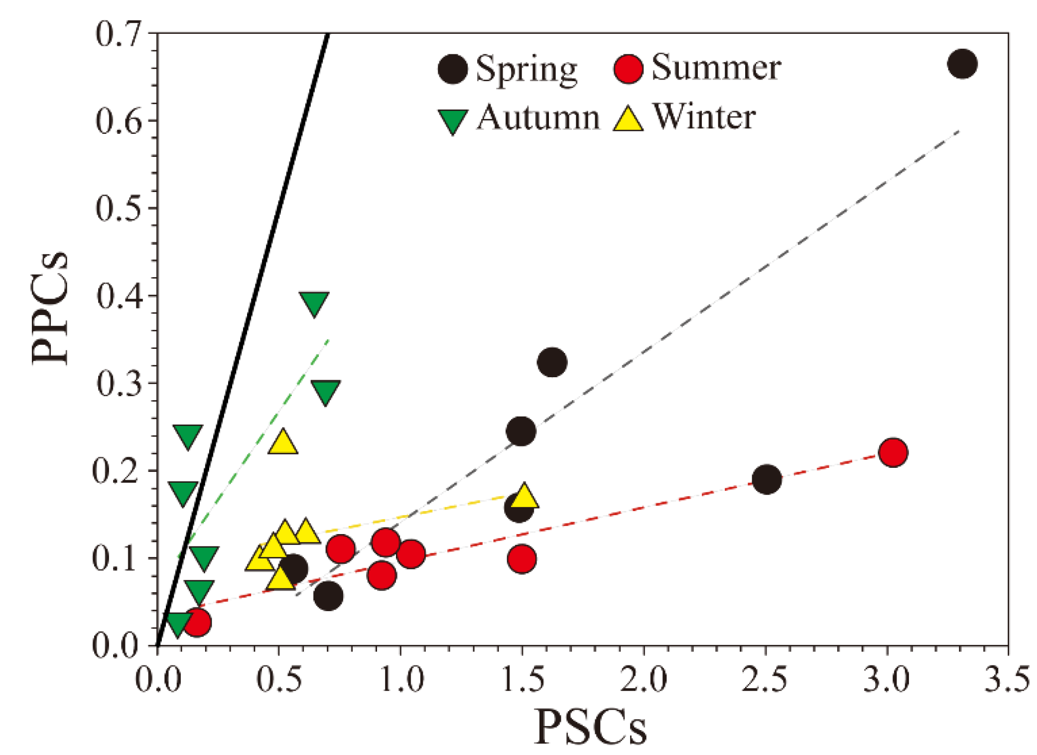
Specific biomarker pigments and particular pigment ratios related to physiological responses to environmental conditions have been used to estimate diverse changes in phytoplankton community structures. Photopigment indices have generally been distinguished into ratio of chlorophylls and carotenoids among total pigments [15], as shown in Table 2. In addition, for carotenoid pigments, the ratio of PPCs to PSC has been used to physiologically characterize autotrophic microalgae [61,62]. Functionally, the total amount of PSCs among all photosynthetic pigments has been considered to be a good indicator, whether it can detect high production areas or not. In contrast, a dominance of PPCs is associated with lower productivity ecosystems [15]. The PSCs to PPCs ratio has been used in estuaries [18,63], the open ocean [23], and coastal areas [21] as an indicator of change in the physiological state of phytoplankton in response to varying ecosystem conditions. In the present study the PPCs to PSCs ratio was relatively low during all seasons other than autumn. The ratio was particularly low in spring and summer, which corresponded to high phytoplankton biomass. However, it was relatively high in autumn, when there were relatively high alloxanthin concentrations and very low fucoxanthin and peridinin concentrations compared with the other seasons (Figure 6).
In spring, the PPCs to PSCs ratio was slightly higher in the upstream area than downstream. In contrast, in summer the PPCs to PSCs ratio was relatively high in the downstream area, where the concentration of PSCs was relatively low. In autumn, no major horizontal differences in the PPCs to PSCs ratio were evident. In winter the ratio was high because of the relatively high concentration of PSCs in the upstream area. Moreno et al. [24] reported a linear relationship between the concentrations of PSCs and PPCs, and found that this ratio was exceptionally low in the shallow waters of the Valdes Peninsula. Conversely, the concentration of PPCs significantly increased under high light intensity and low nutrient conditions, resulting in an increase in the ratio. However, Zhu et al. [64] reported that in spring in the Changjiang (Yangtze) River estuary the PPCs to PSCs ratio was higher than in summer, which was inconsistent with the relative light limitation in spring; an increase in the proportion of diatoms in summer (PPCs : PSCs = 0.09; Table 2) caused a reduction in the ratio. In our study the SRE was dominated by diatoms, so the PSCs concentrations were relatively high. The ratio of PPCs to PSCs was low in all seasons except autumn, implying that the SRE may not be suitable for the growth of phytoplankton in autumn, as reported by Cloern [65] and Lee et al. [25]. These low ratios indicated the SRE is high productivity waters, it was presumed that the maintenance of relatively high primary production in the SRE is heavily influenced by the extensive growth of phytoplankton in Gwangyang Bay [25,47]. Overall, the low PPCs to PSCs ratio in the SRE was related to high diatom biomass. The inner estuarine area may have been influenced by diatom production in the outer bay, suggesting that this may be an important ecological factor in the seasonal phytoplankton population dynamics in the SRE. As a result, it is necessary to continuously study on these indicators of the environmental status in estuary ecosystems in order to identify water quality and ecological changes due to climate change and human activities. Acquiring continuous data may assist development of an ecological habitat index, and aid assessment of the effects of environmental conditions on the complex estuarine and coastal waters for a sustainable environment.
5. Conclusions
We evaluated the phytoplankton community using microscopy and HPLC pigment analyses. The analyzed pigments were used to calculate the pigment indexes (PPCs and PSCs) for functional community structures. Both analyses showed comparable trends in terms of the phytoplankton community. However, the analyses gave quite different results for some of the small non-dominant phytoplankton species including prasinophytes, cyanobacteria, and chlorophytes, which are difficult to identify by microscopy. However, they are important features of estuaries, so their detection is essential in ecological evaluations. The seasonal and horizontal variations in the phytoplankton communities were clearly influenced by the environmental characteristics of SRE, particularly the salinity and nutrient loadings (especially the nitrate+nitrite and silicate concentrations). Both microscopy and the CHEMTAX analyses showed that diatoms dominated in most seasons, while cryptophytes dominated in autumn. However, the microscopy analysis differed in terms of the seasonally and spatially dominant species detected. The ratio of PPCs to PSCs was significantly lower in the SRE compared with other waters. This ratio of PPCs to PSCs in SRE could represents high primary productivity. This was because the ratio in the SRE was dominated by diatom biomass, which has a very low PPCs to PSCs ratio. The high diatom biomass indicates that the area generally has high productivity, but it is likely that this biomass formed in the outer bay but contributed to the phytoplankton biomass of the inner estuarine area. The PPCs to PSCs ratio was slightly higher in autumn and winter, and very low in spring and summer. These seasonal differences were most strongly influenced by the high concentrations of PSCs associated with diatoms. The complementary use of microscopy and HPLC/CHEMTAX analyses allowed for a greater understanding of the SRE ecosystem in terms of productivity and phytoplankton community analysis.
Author Contributions
Data curation, formal analysis, investigation and writing—original draft—M.L.; Data curation and writing—review & editing—N.-I.W.; Conceptualization, funding acquisition and investigation —S.H.B. All authors have read and agreed to the published version of the manuscript.
Funding
This research was supported by the Basic Core Technology Development Program for the Oceans and the Polar Regions of the National Research Foundation (NRF) funded by the Ministry of Science, ICT & Future Planning (grant number NRF-2016M1A5A1027456) and a KIOST projects (PE99812).
Conflicts of Interest
The authors declare no conflict of interest.
References
- Cloern, J.E.; Jassby, A.D.; Schraga, T.S.; Nejad, E.; Martin, C. Ecosystem variability along the estuarine salinity gradient: Examples from long-term study of San Francisco Bay. Limnol. Oceanogr. 2017, 62, 272–291. [Google Scholar] [CrossRef] [Green Version]
- Muylaert, K.; Sabbe, K.; Vyverman, W. Spatial and temporal dynamics of phytoplankton communities in a freshwater tidal estuary (Schelde, Belgium). Estuar. Coast. Shelf. Sci. 2000, 50, 673–687. [Google Scholar] [CrossRef]
- Sheaves, M.; Baker, R.; Nagelkerken, I.; Connolly, R.M. True value of estuarine and coastal nurseries for fish: Incorporating complexity and dynamics. Estuar. Coast. 2015, 38, 401–414. [Google Scholar] [CrossRef] [Green Version]
- Jouenne, F.; Lefebvre, S.; Véron, B.; Lagadeuc, Y. Phytoplankton community structure and primary production in small intertidal estuarine-bay ecosystem (eastern English Channel, France). Mar. Biol. 2007, 151, 805–825. [Google Scholar] [CrossRef]
- Mendiguchía, C.; Moreno, C.; García-Vargas, M. Evaluation of natural and anthropogenic influences on the Guadalquivir River (Spain) by dissolved heavy metals and nutrients. Chemosphere 2007, 69, 1509–1517. [Google Scholar] [CrossRef] [PubMed]
- Yegemova, S.; Kumar, R.; Abuduwaili, J.; Ma, L.; Samat, A.; Issanova, G.; Rodrigo-Comino, J. Identifying the key information and land management plans for water conservation under dry weather conditions in the Border areas of the Syr Darya River in Kazakhstan. Water 2018, 10, 1754. [Google Scholar] [CrossRef] [Green Version]
- Lehman, P.W. The influence of climate on phytoplankton community biomass in San Francisco Bay Estuary. Limnol. Oceanogr. 2000, 45, 580–590. [Google Scholar] [CrossRef] [Green Version]
- Statham, P.J. Nutrients in estuaries—an overview and the potential impacts of climate change. Sci. Total Environ. 2012, 434, 213–227. [Google Scholar] [CrossRef]
- Wolanski, E.; Elliott, M. Estuarine Ecohydrology: An Introduction; Elsevier: Amsterdam, The Netherlands, 2015. [Google Scholar]
- Aktan, Y.; Tüfekçi, V.; Tüfekçi, H.; Aykulu, G. Distribution patterns, biomass estimates and diversity of phytoplankton in Izmit Bay (Turkey). Estuar. Coast. Shelf. Sci. 2005, 64, 372–384. [Google Scholar] [CrossRef]
- Naik, R.K.; Anil, A.C.; Narale, D.D.; Chitari, R.R.; Kulkarni, V.V. Primary description of surface water phytoplankton pigment patterns in the Bay of Bengal. J. Sea. Res. 2011, 65, 435–441. [Google Scholar] [CrossRef]
- Jeffrey, S.W.; Mantoura, R.F.C.; Bjørnland, T. Data for the identification of 47 key phytoplankton pigments. In Phytoplankton Pigments in Oceanography: Guidelines to Modern Methods. Monographs on Oceanographic Methodology; Jeffrey, S.W., Mantoura, R.F.C., Wright, S.W., Eds.; UNESCO: Paris, French, 1997. [Google Scholar]
- Havskum, H.; Schlüter, L.; Scharek, R.; Berdalet, E.; Jacquet, S. Routine quantification of phytoplankton groups microscopy or pigment analyses? Mar. Ecol. Prog. Ser. 2004, 273, 31–42. [Google Scholar] [CrossRef]
- Wright, S.W.; Jeffrey, S.W. Pigment Markers for Phytoplankton Production Marine Organic Matter: Biomarkers, Isotopes and DNA; Springer: Berlin/Heidelberg, Germany, 2006. [Google Scholar]
- Barlow, R.; Kyewalyanga, M.; Sessions, H.; Van den Berg, M.; Morris, T. Phytoplankton pigments, functional types, and absorption properties in the Delagoa and Natal Bights of the Agulhas ecosystem. Estuar. Coast. Shelf Sci. 2008, 80, 201–211. [Google Scholar] [CrossRef]
- Paerl, H.W.; Valdes, L.M.; Pinckney, J.L.; Piehler, M.F.; Dyble, J.; Moisander, P.H. Phytoplankton photopigments as indicators of estuarine and coastal eutrophication. BioScience 2003, 53, 953–964. [Google Scholar] [CrossRef] [Green Version]
- Descy, J.P.; Higgins, H.W.; Mackey, D.J.; Hurley, J.P.; Frost, T.M. Pigment ratios and phytoplankton assessment in northern Wisconsin lakes. J. Phycol. 2000, 36, 274–286. [Google Scholar] [CrossRef]
- Seoane, S.; Garmendia, M.; Revilla, M.; Borja, Á.; Franco, J.; Orive, E.; Valencia, V. Phytoplankton pigments and epifluorescence microscopy as tools for ecological status assessment in coastal and estuarine waters, within the Water Framework Directive. Mar. Pollut. Bull. 2011, 62, 1484–1497. [Google Scholar] [CrossRef]
- Tett, P.; Carreira, C.; Mills, D.K.; Van Leeuwen, S.; Foden, J.; Bresnan, E.; Gowen, R.J. Use of a Phytoplankton Community Index to assess the health of coastal waters. ICES J. Mar. Sci. 2008, 65, 1475–1482. [Google Scholar] [CrossRef]
- Devlin, M.; Barry, J.; Painting, S.; Best, M. Extending the phytoplankton tool kit for the UK Water Framework Directive: Indicators of phytoplankton community structure. Hydrobiologia 2009, 633, 151–168. [Google Scholar] [CrossRef]
- Roy, R.; Pratihary, A.; Mangesh, G.; Naqvi, S.W.A. Spatial variation of phytoplankton pigments along the southwest coast of India. Estuar. Coast. Shelf. Sci. 2006, 69, 189–195. [Google Scholar] [CrossRef]
- Chai, C.; Jiang, T.; Cen, J.; Ge, W.; Lu, S. Phytoplankton pigments and functional community structure in relation to environmental factors in the Pearl River Estuary. Oceanologia 2016, 58, 201–211. [Google Scholar] [CrossRef] [Green Version]
- Gibb, S.W.; Barlow, R.G.; Cummings, D.G.; Rees, N.W.; Trees, C.C.; Holligan, P.; Suggett, D. Surface phytoplankton pigment distributions in the Atlantic Ocean: An assessment of basin scale variability between 50 N and 50 S. Prog. Oceanogr. 2000, 45, 339–368. [Google Scholar] [CrossRef]
- Moreno, D.V.; Marrero, J.P.; Morales, J.; García, C.L.; Úbeda, M.G.V.; Rueda, M.J.; Llinás, O. Phytoplankton functional community structure in Argentinian continental shelf determined by HPLC pigment signatures. Estuar. Coast. Shelf. Sci. 2012, 100, 72–81. [Google Scholar] [CrossRef]
- Lee, M.; Park, B.S.; Baek, S.H. Tidal influences on biotic and abiotic factors in the Seomjin River Estuary and Gwangyang Bay, Korea. Estuaries Coast 2018, 41, 1977–1993. [Google Scholar] [CrossRef]
- Lee, D.I.; Park, C.K.; Cho, H.S. Ecological modeling for water quality management of Kwangyang Bay, Korea. J. Environ. Manag. 2005, 74, 327–337. [Google Scholar] [CrossRef] [PubMed]
- Hwang, J.H.; Jang, D.; Kim, Y.H. Stratification and salt-wedge in the Seomjin river estuary under the idealized tidal influence. Ocean Sci. J. 2017, 52, 469–487. [Google Scholar] [CrossRef]
- Hong, S.H.; Kannan, N.; Yim, U.H.; Choi, J.W.; Shim, W.J. Polychlorinated biphenyls (PCBs) in a benthic ecosystem in Gwangyang Bay, South Korea. Mar. Pollut. Bull. 2011, 62, 2863–2868. [Google Scholar] [CrossRef]
- Zapata, M.; Rodríguez, F.; Garrido, J.L. Separation of chlorophylls and carotenoids from marine phytoplankton: A new HPLC method using a reversed phase C8 column and pyridine-containing mobile phases. Mar. Ecol. Prog. Ser. 2000, 195, 29–45. [Google Scholar] [CrossRef] [Green Version]
- Mackey, M.D.; Mackey, D.J.; Higgins, H.W.; Wright, S.W. CHEMTAX-a program for estimating class abundances from chemical markers: Application to HPLC measurements of phytoplankton. Mar. Ecol. Prog. Ser. 1996, 144, 265–283. [Google Scholar] [CrossRef] [Green Version]
- Riegman, R.; Kraay, G.W. Phytoplankton community structure derived from HPLC analysis of pigments in the Faroe-Shetland Channel during summer 1999: The distribution of taxonomic groups in relation to physical/chemical conditions in the photic zone. J. Plankton Res. 2001, 23, 191–205. [Google Scholar] [CrossRef]
- Zhang, J. Analysis between vegetation and environments I: CCA and DCCA. J. Shanxi Univ. 1992, 15, 182–189. [Google Scholar]
- Tester, P.A.; Geesey, M.E.; Guo, C.; Paerl, H.W.; Millie, D.F. Evaluating phytoplankton dynamics in the Newport River estuary (North Carolina, USA) by HPLC-derived pigment profiles. Mar. Ecol. Prog. Ser. 1995, 124, 237–245. [Google Scholar] [CrossRef] [Green Version]
- Andersen, R.A.; Bidigare, R.R.; Keller, M.D.; Latasa, M. A comparison of HPLC pigment signatures and electron microscopic observations for oligotrophic waters of the North Atlantic and Pacific Oceans. Deep Sea Res. Part Ii Top. Stud. Oceanogr. 1996, 43, 517–537. [Google Scholar] [CrossRef]
- Suzuki, K.; Minami, C.; Liu, H.; Saino, T. Temporal and spatial patterns of chemotaxonomic algal pigments in the subarctic Pacific and the Bering Sea during the early summer of 1999. Deep Sea Res. Part Ii Top. Stud. Oceanogr. 2002, 49, 5685–5704. [Google Scholar] [CrossRef]
- Silva, A.; Mendes, C.; Palma, S.; Brotas, V. Short-time scale variation of phytoplankton succession in Lisbon bay (Portugal) as revealed by microscopy cell counts and HPLC pigment analysis. Estuar. Coast. Shelf. Sci. 2008, 79, 230–238. [Google Scholar] [CrossRef]
- Brewin, R.J.; Sathyendranath, S.; Hirata, T.; Lavender, S.J.; Barciela, R.M.; Hardman-Mountford, N.J. A three-component model of phytoplankton size class for the Atlantic Ocean. Ecol. Model. 2010, 221, 1472–1483. [Google Scholar] [CrossRef]
- Rodrıguez, F.; Pazos, Y.; Maneiro, J.; Zapata, M. Temporal variation in phytoplankton assemblages and pigment composition at a fixed station of the Rıa of Pontevedra (NW Spain). Estuar. Coast. Shelf. Sci. 2003, 58, 499–515. [Google Scholar] [CrossRef]
- Gameiro, C.; Cartaxana, P.; Brotas, V. Environmental drivers of phytoplankton distribution and composition in Tagus Estuary, Portugal. Estuar. Coast. Shelf. Sci. 2007, 75, 21–34. [Google Scholar] [CrossRef]
- Olenina, I. Biovolumes and size-classes of phytoplankton in the Baltic Sea. Baltic Sea Environ. Proc. 2006, 106, 1–144. [Google Scholar]
- Schlüter, L.; Møhlenberg, F.; Havskum, H.; Larsen, S. The use of phytoplankton pigments for identifying and quantifying phytoplankton groups in coastal areas: Testing the influence of light and nutrients on pigment/chlorophyll a ratios. Mar. Ecol. Prog. Ser. 2000, 192, 49–63. [Google Scholar] [CrossRef] [Green Version]
- Lignell, R. Excretion of organic carbon by phytoplankton: Its relation to algal biomass, primary productivity and bacterial secondary productivity in the Baltic Sea. Mar. Ecol. Prog. Ser. 1990, 68, 85–99. [Google Scholar] [CrossRef]
- Huot, Y.; Babin, M.; Bruyant, F.; Grob, C.; Twardowski, M.S.; Claustre, H. Does chlorophyll a provide the best index of phytoplankton biomass for primary productivity studies? Biogeosci. Discuss. 2007, 4, 707–745. [Google Scholar] [CrossRef] [Green Version]
- Kasprzak, P.; Padisák, J.; Koschel, R.; Krienitz, L.; Gervais, F. Chlorophyll a concentration across a trophic gradient of lakes: An estimator of phytoplankton biomass? Limnologica 2008, 38, 327–338. [Google Scholar] [CrossRef] [Green Version]
- Breton, E.; Brunet, C.; Sautour, B.; Brylinski, J.M. Annual variations of phytoplankton biomass in the Eastern English Channel: Comparison by pigment signatures and microscopic counts. J. Plankton Res. 2000, 22, 1423–1440. [Google Scholar] [CrossRef] [Green Version]
- Ediger, D.; Soydemir, N.; Kideys, A.E. Estimation of phytoplankton biomass using HPLC pigment analysis in the southwestern Black Sea. Deep Sea Res. Part Ii Top. Stud. Oceanogr. 2006, 53, 1911–1922. [Google Scholar] [CrossRef]
- Baek, S.H.; Kim, D.; Son, M.; Yun, S.M.; Kim, Y.O. Seasonal distribution of phytoplankton assemblages and nutrient-enriched bioassays as indicators of nutrient limitation of phytoplankton growth in Gwangyang Bay, Korea. Estuar. Coast. Shelf. Sci. 2015, 163, 265–278. [Google Scholar] [CrossRef]
- Park, T.G.; Lim, W.A.; Park, Y.T.; Lee, C.K.; Jeong, H.J. Economic impact, management and mitigation of red tides in Korea. Harmful algae 2013, 30, 131–143. [Google Scholar] [CrossRef]
- Baek, S.H.; Shin, K.; Son, M.; Bae, S.W.; Cho, H.; Na, D.H.; Kim, Y.O.; Kim, S.W. Algicidal effects of yellow clay and the thiazolidinedione derivative TD49 on the fish-killing dinoflagellate Cochlodinium polykrikoides in microcosm experiments. J. Appl. Phycol. 2014, 26, 2367–2378. [Google Scholar] [CrossRef]
- Tolotti, M.; Corradini, F.; Boscaini, A.; Calliari, D. Weather-driven ecology of planktonic diatoms in Lake Tovel (Trentino, Italy). Hydrobiologia 2007, 578, 147–156. [Google Scholar] [CrossRef]
- Hötzel, G.; Croome, R. Population dynamics of Aulacoseira granulata (EHR.) SIMONSON (Bacillariophyceae, Centrales), the dominant alga in the Murray River, Australia. Arch. Hydrobiol. 1996, 136, 191–215. [Google Scholar]
- Wang, C.; Li, X.; Lai, Z.; Tan, X.; Pang, S.; Yang, W. Seasonal variations of Aulacoseira granulata population abundance in the Pearl River Estuary. Estuar. Coast. Shelf Sci. 2009, 85, 585–592. [Google Scholar] [CrossRef]
- Na, J.-E.; Jung, M.-H.; Cho, I.-S.; Park, J.-H.; Hwang, K.-S.; Song, H.-J.; Lim, B.-J.; La, G.-H.; Kim, H.-W.; Lee, H.-Y. Phytoplankton community in reservoirs of Yeongsan and Seomjin River basins, Korea. Korean J. Environ. Biol. 2012, 30, 39–46. [Google Scholar]
- Yu, J.J.; Lee, H.J.; Lee, K.L.; Lyu, H.S.; Whang, J.W.; Shin, L.Y.; Chen, S.U. Relationship between distribution of the dominant phytoplankton species and water temperature in the Nakdong River, Korea. Korean J. Environ. Ecol. 2014, 47, 247–257. [Google Scholar] [CrossRef]
- Sommer, U. Comparison between steady state and non-steady state competition: Experiments with natural phytoplankton. Limnol. Oceanogr. 1985, 30, 335–346. [Google Scholar] [CrossRef]
- Klaveness, D. Biology and ecology of the Cryptophyceae: Status and challenges. Biol. Oceanog. 1989, 6, 257–270. [Google Scholar]
- Barone, R.; Naselli-Flores, L. Distribution and seasonal dynamics of Cryptomonads in Sicilian water bodies. Hydrobiologia 2003, 502, 325–329. [Google Scholar] [CrossRef]
- Baek, S.H.; Kim, D.; Kim, Y.O.; Son, M.; Kim, Y.-J.; Lee, M.; Park, B.S. Seasonal changes in abiotic environmental conditions in the Busan coastal region (South Korea) due to the Nakdong River in 2013 and effect of these changes on phytoplankton communities. Cont. Shelf Res. 2019, 175, 116–126. [Google Scholar] [CrossRef]
- Kaeriyama, H.; Katsuki, E.; Otsubo, M.; Yamada, M.; Ichimi, K.; Tada, K.; Harrison, P.J. Effects of temperature and irradiance on growth of strains belonging to seven Skeletonema species isolated from Dokai Bay, southern Japan. Eur. J. Phycol. 2011, 46, 113–124. [Google Scholar] [CrossRef] [Green Version]
- Smayda, T.J. Harmful algal blooms: Their ecophysiology and general relevance to phytoplankton blooms in the sea. Limnol. Oceanogr. 1997, 42, 1137–1153. [Google Scholar] [CrossRef]
- Bidigare, R.R.; Ondrusek, M.E. Spatial and temporal variability of phytoplankton pigment distributions in the central equatorial Pacific Ocean. Deep Sea Res. Part Ii Top. Stud. Oceanogr. 1996, 43, 809–833. [Google Scholar] [CrossRef]
- Madhu, N.; Ullas, N.; Ashwini, R.; Meenu, P.; Rehitha, T.; Lallu, K. Characterization of phytoplankton pigments and functional community structure in the Gulf of Mannar and the Palk Bay using HPLC–CHEMTAX analysis. Cont. Shelf Res. 2014, 80, 79–90. [Google Scholar] [CrossRef]
- Wysocki, L.A.; Bianchi, T.S.; Powell, R.T.; Reuss, N. Spatial variability in the coupling of organic carbon, nutrients, and phytoplankton pigments in surface waters and sediments of the Mississippi River plume. Estuar. Coast. Shelf Sci. 2006, 69, 47–63. [Google Scholar] [CrossRef]
- Zhu, Z.-Y.; Ng, W.-M.; Liu, S.-M.; Zhang, J.; Chen, J.-C.; Wu, Y. Estuarine phytoplankton dynamics and shift of limiting factors: A study in the Changjiang (Yangtze River) Estuary and adjacent area. Estuar. Coast. Shelf Sci. 2009, 84, 393–401. [Google Scholar] [CrossRef]
- Cloern, J.E. Turbidity as a control on phytoplankton biomass and productivity in estuaries. Cont. Shelf Res. 1987, 7, 1367–1381. [Google Scholar] [CrossRef]
Figure 1.
Study area and sampling stations in the Seomjin River estuary (SRE) and Gwangyang Bay.

Figure 2.
Horizontal distribution of concentration of pigments in the SRE. (A) Spring, (B) Summer, (C) Autumn, (D) Winter. Abbreviations of each pigment are listed in Table 1.
Figure 2.
Horizontal distribution of concentration of pigments in the SRE. (A) Spring, (B) Summer, (C) Autumn, (D) Winter. Abbreviations of each pigment are listed in Table 1.

Figure 3.
The contribution of each taxonomic group to total phytoplankton biomass, calculated using CHEMTAX, and the total chl-a by pigment analysis. (A) Spring, (B) Summer, (C) Autumn, (D) Winter.
Figure 3.
The contribution of each taxonomic group to total phytoplankton biomass, calculated using CHEMTAX, and the total chl-a by pigment analysis. (A) Spring, (B) Summer, (C) Autumn, (D) Winter.

Figure 4.
Relationship between (A) the fucoxanthin concentration and diatom abundance, (B) alloxanthin and the cryptophyte abundance, and (C) peridinin and the dinoflagellate abundance. The thick line indicates the trend line for all seasons. The dotted lines indicate the seasonal trend lines.
Figure 4.
Relationship between (A) the fucoxanthin concentration and diatom abundance, (B) alloxanthin and the cryptophyte abundance, and (C) peridinin and the dinoflagellate abundance. The thick line indicates the trend line for all seasons. The dotted lines indicate the seasonal trend lines.

Figure 5.
Canonical correspondence analysis (CCA) biplots of the phytoplankton community and environmental factors in the SRE. (A) Spring, (B) Summer, (C) Autumn, (D) Winter, and (E) all seasons combined. S.: spring; Sm.: summer; A.: Autumn; W.: winter; Temp.: temperature; Sal.: salinity; Dino.: dinoflagellates; Chloro.: chlorophytes; Crypto.: cryptophytes; Cyano.: cyanobacteria; Hapto.: haptophytes; Prasino.: prasinophytes.

Figure 6.
Relationship between the concentrations of photoprotective carotenoids (PPCs) and photosynthetic carotenoid pigments (PSCs) in the SRE. The thick line indicates a PPCs:PSCs ratio of 1. The dotted lines indicate the seasonal trend lines.
Figure 6.
Relationship between the concentrations of photoprotective carotenoids (PPCs) and photosynthetic carotenoid pigments (PSCs) in the SRE. The thick line indicates a PPCs:PSCs ratio of 1. The dotted lines indicate the seasonal trend lines.


Table 1.
Abbreviations, names, formula, and selected taxonomic designations for chlorophylls, carotenoids, and pigment combinations and indices.
Table 1.
Abbreviations, names, formula, and selected taxonomic designations for chlorophylls, carotenoids, and pigment combinations and indices.
| Abbreviations | Pigment | Designation |
| Chl-a | Chlorophyll a | |
| Chl-c2 | Chlorophyll c2 | |
| Chl-b | Chlorophyll b | Chlorophytes |
| Allo | Alloxanthin | Cryptophytes |
| Diad | Diadinoxanthin | |
| Diato | Diatoxanthin | |
| Fuco | Fucoxathin | Diatoms (major) |
| Hex | 19’ Hexanoyloxy fucoxanthin | Prymnesiophytes |
| Peri | Peridinine | Dinoflagellates |
| Zea | Zeaxanthin | Cyanobacteria |
| Β-Car | β-Carotene | |
| But | 19’ Butanoyloxy fucoxanthin | Haptophytes (major) |
| Viol | Violaxanthin | |
| Lut | Lutein | |
| Neo | 9’-cis-neoxanthin | |
| Variable | Pigment sum | Formula |
| TChl-a | Total chlorophyll a | Chl a+DVChl a+Chlide a |
| PPCs | Photoprotective carotenoids | Allo+Diad+Vio+Zea+β−Car |
| PSCs | Photosynthetic carotenoids | But+Fuco+Hex+Per |
Table 2.
Initial pigment ratios used for the CHEMTAX analysis. Pras: Prasinophytes; Dino: Dinoflagellates; Crypto: Cryptophytes; Hapto_N: Haptophytes; Hapto_S: Chrysophytes; Chloro: Chlorophytes; Cyano: Cyanobacteria; Diat: Diatoms. Abbreviations of each pigment are listed in Table 1.
Table 2.
Initial pigment ratios used for the CHEMTAX analysis. Pras: Prasinophytes; Dino: Dinoflagellates; Crypto: Cryptophytes; Hapto_N: Haptophytes; Hapto_S: Chrysophytes; Chloro: Chlorophytes; Cyano: Cyanobacteria; Diat: Diatoms. Abbreviations of each pigment are listed in Table 1.
| Perid | 19butfu | Fuco | 19hexfu | Neo | Prasino | Viol | Allo | Lut | Zea | Chl b | |
|---|---|---|---|---|---|---|---|---|---|---|---|
| Prasino | 0 | 0 | 0 | 0 | 0.3768 | 0.1413 | 0.2165 | 0 | 0.0843 | 0 | 0.2807 |
| Dino | 0.7471 | 0 | 0 | 0 | 0 | 0 | 0 | 0 | 0 | 0 | 0 |
| Crypto | 0 | 0 | 0 | 0 | 0 | 0 | 0 | 0.1927 | 0 | 0 | 0 |
| Hapto_N | 0 | 0 | 0 | 1.7139 | 0 | 0 | 0 | 0 | 0 | 0 | 0 |
| Hapto_S | 0 | 0.5076 | 0.8354 | 0.2225 | 0 | 0 | 0 | 0 | 0 | 0 | 0 |
| Chloro | 0 | 0 | 0 | 0 | 0.0495 | 0 | 0.1185 | 0 | 0.1294 | 0.3262 | 0.0168 |
| Cyano | 0 | 0 | 0 | 0 | 0 | 0 | 0 | 0 | 0 | 0.6795 | 0 |
| Diat | 0 | 0 | 1.0198 | 0 | 0 | 0 | 0 | 0 | 0 | 0 | 0 |
Table 3.
Seasonal environmental characteristics at the sampling stations in the SRE (S: spring; Sm: summer; A: autumn; W: winter). Precipitation: accumulated precipitation in the 10 days prior to the sampling date; Discharge: mean water discharge in the 7 days prior to the sampling date; Temp.: temperature; Sal.: salinity; DO: dissolved oxygen; NOx: nitrate+nitrite concentration; NH4+: ammonium; DIP: dissolved inorganic phosphate; DSi: silicate concentration.
| Precipitation | Discharge | Temp. | Sal. | DO | NOx | NH4+ | DIP | DSi | |
|---|---|---|---|---|---|---|---|---|---|
| (mm/10days) | (m3 s−1) | (°C) | (psu) | (mg L−1) | (uM) | (uM) | (uM) | (uM) | |
| S1 | 17.7 | 5.5 | 20.16 | 33.05 | 6.88 | 2.99 | 3.58 | 0.41 | 14.04 |
| S2 | 21.24 | 31.34 | 6.65 | 4.32 | 5.31 | 0.65 | 20.53 | ||
| S3 | 21.45 | 31.75 | 6.32 | 4.77 | 5.86 | 0.69 | 20.18 | ||
| S4 | 22.36 | 27.32 | 6.92 | 15.54 | 6.49 | 0.88 | 36.96 | ||
| S5 | 23.20 | 20.81 | 6.90 | 28.89 | 5.72 | 0.86 | 53.05 | ||
| S6 | 23.50 | 18.44 | 6.58 | 35.54 | 5.60 | 0.87 | 64.08 | ||
| S7 | 23.76 | 12.74 | 7.05 | 39.89 | 3.74 | 0.74 | 64.61 | ||
| Sm1 | 12.8 | 17.5 | 23.25 | 32.03 | 5.74 | 0.96 | 0.39 | 0.35 | 17.63 |
| Sm2 | 25.15 | 30.03 | 6.44 | 1.08 | 2.27 | 0.46 | 18.22 | ||
| Sm3 | 25.68 | 28.74 | 5.96 | 1.33 | 3.58 | 0.53 | 19.49 | ||
| Sm4 | 26.52 | 25.30 | 6.33 | 0.84 | 3.81 | 0.41 | 21.54 | ||
| Sm5 | 26.52 | 21.57 | 6.70 | 2.95 | 4.33 | 0.33 | 32.23 | ||
| Sm6 | 26.60 | 17.08 | 6.76 | 7.15 | 5.27 | 0.34 | 45.88 | ||
| Sm7 | 26.91 | 17.28 | 6.38 | 5.70 | 5.53 | 0.34 | 46.07 | ||
| A1 | 15.4 | 38.5 | 18.23 | 31.76 | 7.58 | 2.34 | 5.69 | 0.94 | 14.48 |
| A2 | 18.05 | 29.88 | 7.90 | 6.07 | 7.30 | 1.06 | 25.13 | ||
| A3 | 17.69 | 27.81 | 7.88 | 6.70 | 7.40 | 1.08 | 24.27 | ||
| A4 | 16.95 | 22.65 | 7.64 | 12.06 | 7.03 | 1.10 | 36.14 | ||
| A5 | 16.45 | 15.30 | 8.20 | 22.78 | 6.15 | 0.98 | 55.81 | ||
| A6 | 16.27 | 14.67 | 8.33 | 23.49 | 5.77 | 0.77 | 48.61 | ||
| A7 | 15.90 | 9.90 | 8.92 | 28.75 | 5.23 | 0.84 | 62.48 | ||
| W1 | 46.9 | 69.0 | 7.88 | 31.71 | 10.26 | 2.71 | 0.88 | 0.31 | 8.17 |
| W2 | 8.00 | 30.25 | 10.11 | 7.77 | 1.90 | 0.35 | 16.95 | ||
| W3 | 7.96 | 27.68 | 10.30 | 10.41 | 2.09 | 0.36 | 20.23 | ||
| W4 | 7.25 | 22.20 | 10.88 | 28.37 | 2.37 | 0.28 | 45.98 | ||
| W5 | 6.88 | 14.69 | 11.47 | 44.51 | 1.86 | 0.26 | 62.95 | ||
| W6 | 7.11 | 15.20 | 11.50 | 45.17 | 2.01 | 0.27 | 63.89 | ||
| W7 | 6.36 | 9.80 | 11.80 | 58.48 | 1.58 | 0.23 | 74.19 |
Table 4.
Seasonal abundance (×105 cells L−1) and percentage community composition of phytoplankton.
| Station 1 | Station 2 | Station 3 | Station 4 | Station 5 | Station 6 | Station 7 | ||
|---|---|---|---|---|---|---|---|---|
| Spring | Total abundance | 9.05 | 2.01 | 2.68 | 1.85 | 2.40 | 2.50 | 7.11 |
| Diatoms (%) | 84.70 | 73.86 | 72.98 | 53.74 | 27.06 | 43.29 | 18.95 | |
| Dinoflagellates (%) | 0.53 | 2.90 | 0.31 | 0.93 | 0.00 | 0.61 | 2.15 | |
| Cryptophytes (%) | 14.41 | 23.24 | 26.40 | 44.86 | 72.61 | 56.10 | 78.78 | |
| Summer | Total abundance | 2.72 | 0.69 | 1.07 | 2.17 | 4.83 | 4.81 | 7.15 |
| Diatoms (%) | 62.86 | 76.73 | 81.12 | 84.24 | 89.28 | 85.89 | 83.77 | |
| Dinoflagellates (%) | 33.97 | 9.43 | 8.03 | 7.27 | 3.72 | 4.53 | 2.07 | |
| Cryptophytes (%) | 3.17 | 13.84 | 10.84 | 8.18 | 6.56 | 9.07 | 11.23 | |
| Autumn | Total abundance | 1.80 | 1.34 | 2.16 | 2.12 | 2.37 | 3.83 | 0.93 |
| Diatoms (%) | 10.19 | 9.52 | 4.92 | 1.33 | 5.41 | 5.81 | 3.89 | |
| Dinoflagellates (%) | 1.85 | 0.00 | 0.00 | 0.67 | 0.00 | 1.66 | 0.56 | |
| Cryptophytes (%) | 87.04 | 89.29 | 95.08 | 96.00 | 94.59 | 91.29 | 94.44 | |
| Winter | Total abundance | 5.22 | 2.20 | 2.31 | 2.36 | 1.56 | 2.67 | 2.93 |
| Diatoms (%) | 96.71 | 91.94 | 85.71 | 79.53 | 83.33 | 96.08 | 95.06 | |
| Dinoflagellates (%) | 0.00 | 0.81 | 0.00 | 0.00 | 0.00 | 0.00 | 1.23 | |
| Cryptophytes (%) | 2.74 | 4.84 | 11.43 | 19.69 | 15.56 | 3.27 | 2.47 |
Table 5.
Dominant seasonal phytoplankton genera and relative abundance.
| Station 1 | Station 2 | Station 3 | Station 4 | Station 5 | Station 6 | Station 7 | ||
|---|---|---|---|---|---|---|---|---|
| Spring | Chaetoceros | +++ | ++ | ++ | ++ | ++ | ++ | ++ |
| Skeletonema | ++ | + | + | ++ | + | ++ | ++ | |
| Thalassionema | +++ | ++ | +++ | ++ | ++ | + | + | |
| Cryptomonas | +++ | ++ | ++ | ++ | +++ | +++ | +++ | |
| Summer | Aulacoseira | + | ++ | ++ | +++ | +++ | +++ | |
| Chaetoceros | ++ | ++ | ++ | ++ | ++ | ++ | ++ | |
| Skeletonema | ++ | + | ++ | ++ | ++ | ++ | ++ | |
| Cryptomonas | + | ++ | ++ | ++ | ++ | ++ | ++ | |
| Autumn | Amphora | + | + | + | ||||
| Navicular | ++ | + | + | + | + | + | ||
| Nitzschia | + | + | + | + | + | |||
| Cryptomonas | +++ | +++ | +++ | +++ | +++ | +++ | +++ | |
| Winter | Chaetoceros | +++ | ++ | ++ | ++ | ++ | ++ | ++ |
| Skeletonema | +++ | ++ | +++ | +++ | ++ | +++ | +++ | |
| Thalassiosira | ++ | ++ | + | ++ | ++ | ++ | ++ | |
| Cryptomonas | ++ | ++ | ++ | ++ | ++ | + | + |
+ <103; ++ <104; +++ >104 (cells L−1).
© 2020 by the authors. Licensee MDPI, Basel, Switzerland. This article is an open access article distributed under the terms and conditions of the Creative Commons Attribution (CC BY) license (http://creativecommons.org/licenses/by/4.0/).
Share and Cite
MDPI and ACS Style
Lee, M.; Won, N.-I.; Baek, S.H. Comparison of HPLC Pigment Analysis and Microscopy in Phytoplankton Assessment in the Seomjin River Estuary, Korea. Sustainability 2020, 12, 1675. https://0-doi-org.brum.beds.ac.uk/10.3390/su12041675
AMA Style
Lee M, Won N-I, Baek SH. Comparison of HPLC Pigment Analysis and Microscopy in Phytoplankton Assessment in the Seomjin River Estuary, Korea. Sustainability. 2020; 12(4):1675. https://0-doi-org.brum.beds.ac.uk/10.3390/su12041675
Chicago/Turabian StyleLee, Minji, Nam-Il Won, and Seung Ho Baek. 2020. "Comparison of HPLC Pigment Analysis and Microscopy in Phytoplankton Assessment in the Seomjin River Estuary, Korea" Sustainability 12, no. 4: 1675. https://0-doi-org.brum.beds.ac.uk/10.3390/su12041675
Note that from the first issue of 2016, this journal uses article numbers instead of page numbers. See further details here.