Environmental and Economic Water Management in Shale Gas Extraction
by
 , , ,
, , ,
José A. Caballero
1,* ,
,
Juan A. Labarta
1,
Natalia Quirante
1,
Alba Carrero-Parreño
1 and
Ignacio E. Grossmann
2 1
Institute of Chemical Process Engineering, University of Alicante, PO 99, E-03080 Alicante, Spain
2
Department of Chemical Engineering, Carnegie Mellon University, Pittsburgh, PA 15213, USA
*
Author to whom correspondence should be addressed.
Sustainability 2020, 12(4), 1686; https://0-doi-org.brum.beds.ac.uk/10.3390/su12041686
Submission received: 29 January 2020
/
Revised: 14 February 2020
/
Accepted: 21 February 2020
/
Published: 24 February 2020
(This article belongs to the Special Issue Optimization and Big Data Analytics to Improve Profitability and Sustainability of the Oil and Gas Industry)
Abstract
:This paper introduces a comprehensive study of the Life Cycle Impact Assessment (LCIA) of water management in shale gas exploitation. First, we present a comprehensive study of wastewater treatment in the shale gas extraction, including the most common technologies for the pretreatment and three different desalination technologies of recent interest: Single and Multiple-Effect Evaporation with Mechanical Vapor Recompression and Membrane Distillation. The analysis has been carried out through a generic Life Cycle Assessment (LCA) and the ReCiPe metric (at midpoint and endpoint levels), considering a wide range of environmental impacts. The results show that among these technologies Multiple-Effect Evaporation with Mechanical Vapor Recompression (MEE-MVR) is the most suitable technology for the wastewater treatment in shale gas extraction, taking into account its reduced environmental impact, the high water recovery compared to other alternatives as well as the lower cost of this technology. We also use a comprehensive water management model that includes previous results that takes the form of a new Mixed-Integer Linear Programming (MILP) bi-criterion optimization model to address the profit maximization and the minimization Life Cycle Impact Assessment (LCIA), based on its results we discuss the main tradeoffs between optimal operation from the economic and environmental points of view.
1. Introduction
Natural gas extracted from tight shale formations “shale gas” is playing an important role in satisfying the continuous increase in global energy demand. In the last year (2018) the primary energy consumption grew at a rate of 2.9%, which is almost twice its 10 previous-year average growth, which was around 1.5% per year, and it was also the fastest since 2010 [1]. By fuel, energy consumption was driven by natural gas with a contribution greater than 40% of the increase. In 2018 natural gas consumption increased by 195 billion cubic meters (bcm), this is 5.3%, which is one of the fastest growths since 1984 [2].
In the year 2000, the contribution of shale gas to the natural gas production in the United States was close to 1%, in 2010 it was over 20%, and by 2035 is forecasted to be more than 46% [3]. According to a projection of the Energy Information Administration in 2050, the amount of natural gas produced from shale and tight oil formation will be over 75% of the total natural gas production in the United States [4].
The first extraction of shale gas was done in 1821 in Fredonia (New York). However, the horizontal drilling started in the 30s of the last century, and the first well was fractured in the United States in 1947. Since that time, the continuous advances in hydraulic fracturing and horizontal drilling have enhanced technically and economically the exploration of extensive shale gas formations in the United States [5,6,7], and they have significantly altered the global energy scenario for any foreseeable future [8,9]. Curiously, the public attention was focused on this issue only in 2007, when the US Gas Committee increased its estimations of unproven US gas reserves from 32.7 trillion cubic meters (tcm; 1 tcm = 1012 m3) to 47.7 tcm, around 45% [10]. The consequence of the increase in the supply of Natural Gas in the US produced a remarkable drop in the local natural gas prices. In the United States, the average price between 2003 and 2008 was $242.2 per thousand cubic meters ($/Mm3). It decreased to an average of 139.0 $/Mm3 in the period 2009–2011, and further decrease between 2012 and 2018 with an average value of 106.8 $/Mm3 [2]. However, while in the United States the prices of natural gas decreased, in the rest of the world the prices have significantly increased. For example, in the Organisation for Economic Co-operation and Development (OECD) countries, the price increased from the 165.9 $/Mm3 in 2003 to an average value of 614.4 $/Mm3 in the period 2011–2014. Even though prices decreased to an average value of 309.4 $/Mm3 in the period 2015–2018 (with a new important increment in 2018, around 396 $/Mm3) the values are significantly larger than those in the United States [2].
Despite many countries having important reserves of shale gas, only the United States, Canada, China, and to a lesser extension Argentina and Australia, are currently producing shale gas at a commercial scale. For example, Canada, ranked second after the United States with regard to shale gas production 1496.5 billion cubic feet (bcf) in 2015, and it is the only country, apart from the United States, that has achieved commercial level [11]. China has the highest proven reserves of shale gas in the world. They were estimated in 2015 in around 1115.2 tcf (trillion cubic feet), about 15% of the world total. The first shale gas well was drilled in 2010 and in 2016 the production has reached 0.7 bcf per day, which is around 5.4% of the total domestic gas production. According to the Chinese energy development plant, the objective is to reach a 15% share of natural gas by 2030 [11]. In Argentina, the total shale gas production reached 64.6 bcf in 2015 (about 5% of the total natural gas production). Natural gas production from tight sands and shales are expected to continue to grow to account for two-thirds of total domestic natural gas by 2030 and three quarters by 2040 [11].
Interestingly, the success of the shale gas revolution in the United States has not been yet replicated in other countries. For example, in Europe, there is an important public and political opposition to hydraulic fracturing. Concerns on environmental impacts such as groundwater contamination, risk of earthquakes, greenhouse gas emissions, water consumption, or uncertainties about the correct management of water due to improper disposal of flowback and produced water, have led many countries to impose moratoria on shale gas exploration and hence subject to further research [12,13,14].
One of the main environmental concerns of shale gas production is based on the large amount of water needed for the fracturing process. Production of shale gas involves around 7500–38,000 m3 of water per well. Out of this, 90% is required for the fracking process and the remaining 10% is used for horizontal drilling activities [15]. A variable amount of water (between 10% and 80% of the injected fluid [16,17] is recovered in the first two weeks after beginning the process, which is known as “flowback water”. However, the percentage of flowback water reported by other authors is quite different (between 8–15% [18]) and values of 10–40% [19], depending on the geology and the geomechanics of the formation. Thereafter, shale gas produced during the exploitation phase (∼20 years) is accompanied by more water that is continuously recovered, known as “produced water” [20].
Flowback water is mainly composed of total dissolved solids (TDS), total organic carbon (TOC) and total suspended solids (TSS), among others [21,22]. Among all these contaminants, TDS (composed of salts, minerals and scaling ions with concentrations between 10,000 and 200,000 mg·L−1) separation is difficult due to the large amount of energy needed and the possible environmental impacts of high-salinity water disposal [19].
Due to its physical and chemical properties, flowback water can be managed by different strategies, including disposal through Class II disposal wells, dispatch to other destinations such as a centralized water treatment facilities (CWT), or direct reuse in the drilling and fracturing operations of the well or subsequent wells.
Injection in Class II wells is the strategy most used in the USA. In fact, there are many places where local disposal is allowed, which makes the cost of water injection to be inexpensive. However, in other shale sites, there are no Class II wells and long distances must be traveled to inject the wastewater, which increases the cost [8]. It is not clear if, in Europe, injection in wells would be eventually an acceptable alternative for the disposal of flowback water. For example, some reports refer to this decision as a possible solution in the UK [23]. In addition, well injection has been correlated with seismic activity, whose contribution is significantly larger than hydraulic fracturing itself [24].
Nowadays, given the importance of water conservation, the best option is the direct reuse of the flowback water because it allows reducing freshwater consumption and the environmental problems associated with water management, such as transportation, disposal or treatment for its recovery. To guarantee adequate disposal to the environment and the final recovery of water, desalination post-treatment is receiving increased attention. Thus, Shaffer et al. [25] explored all the technical, economic and regulatory drivers that lead to the choice of desalination instead of injection disposal.
Effective desalination processes are needed in order to properly treat the high salinity of flowback water. Desalination processes include membrane-based technologies (such as reverse osmosis (RO) and forward osmosis (FO)) and thermal-based technologies, which comprise multistage flash (MSF) and single/multiple-effect evaporation (SEE/MEE) with/without thermal or mechanical vapor recompression (TVR/MVR). The most used technology in seawater desalination is RO, due to its economic performance. However, RO has the limitation of not being able to be used when TDS concentration is higher than ~40,000–45,000 mg/L [26]. Nevertheless, the critical point of FO is how to choose the right draw solution. Preferably, the desired draw solution has to be relatively cheap, must avoid fouling and have to be capable to provide sufficient high osmotic pressure to create a large flux across the membrane [27]. However, draw solutions have the disadvantage that they must be recovered in additional separation processes, which increase the cost of the process. Some of these limitations where solved combining FO and RO for shale water treatment [28]. Nevertheless, due to these limitations in the desalination of produced water, thermal desalination and membrane distillation are more attractive than membrane processes [25,29], and economically more efficient than membrane technologies. The objective of thermal desalination and membrane distillation is to recover treated water, reducing wastewater discharge and the corresponding water footprint.
Several studies have evaluated the carbon dioxide emissions of water management to estimate the environmental impacts of water and wastewater operations [30,31,32,33]. Just very few works have introduced other impact indicators in their studies, in addition to the global warming potential, such as fossil depletion, particulate matter formation, and human toxicity, among others [34,35,36]. Other studies have been focused on the design of shale gas supply chains for the optimal management of water [20,37,38,39,40].
At this point, it is important to remark that the main application of the previous environmental works was the estimation of greenhouse gas (GHG) emissions and the carbon footprint associated with the manufacture of shale gas [41,42,43]. However, none of these works have focused on studying the different alternatives for wastewater treatment and none of them shows a detailed and specific inventory of wastewater treatment. Therefore, in this paper we first address the life cycle impact assessment (LCIA) of three alternative desalination technologies for wastewater in shale gas extraction: Single-Effect Evaporation with Mechanical Vapor Recompression (SEE-MVR), Multiple-Effect Evaporation with Mechanical Vapor Recompression (MEE-MVR), and Membrane Distillation (MD). We analyze their corresponding LCIAs in order to compare their sustainability. This perspective also includes the analysis of the most common technologies for the initial pre-treatment of this type of wastewater.
Furthermore, this work studies a wide range of environmental impacts, including the global warming potential, acidification potential, resource depletion, toxicities, etc., by using the ReCipe method [44] with different perspectives (mid and endpoint) from Ecoinvent database v.3.4 [45].
In order to compare these new treatment alternatives, which might be promising for wastewater in the shale gas process, this paper is structured as follows: Section 2 introduces the life cycle assessment methodology and shows the alternatives studied for the wastewater treatment. In Section 3, we use the results of previous sections into a complete management model that takes into account the costs and environmental impacts of all activities related to water management in shale gas exploitation. Finally, the conclusions and the list of references are provided at the end of the article.
2. Life Cycle Assessment Methodology
The Life Cycle Assessment (LCA) methodology is the most used technique to evaluate environmental impacts [46,47]. This method considers all the environmental characteristics and the potential impacts related to all phases of a product’s life (that is, the supply of raw materials, the manufacturing of intermediates, and the final product, including storage, packaging, transportation, distribution, use, and disposal of the product) [48]. Moreover, it helps to identify the activities with more negative environmental impacts and what damage categories are more relevant. This analysis allows defining the corresponding set of targets in order to develop more sustainable industrial processes and practices [48].
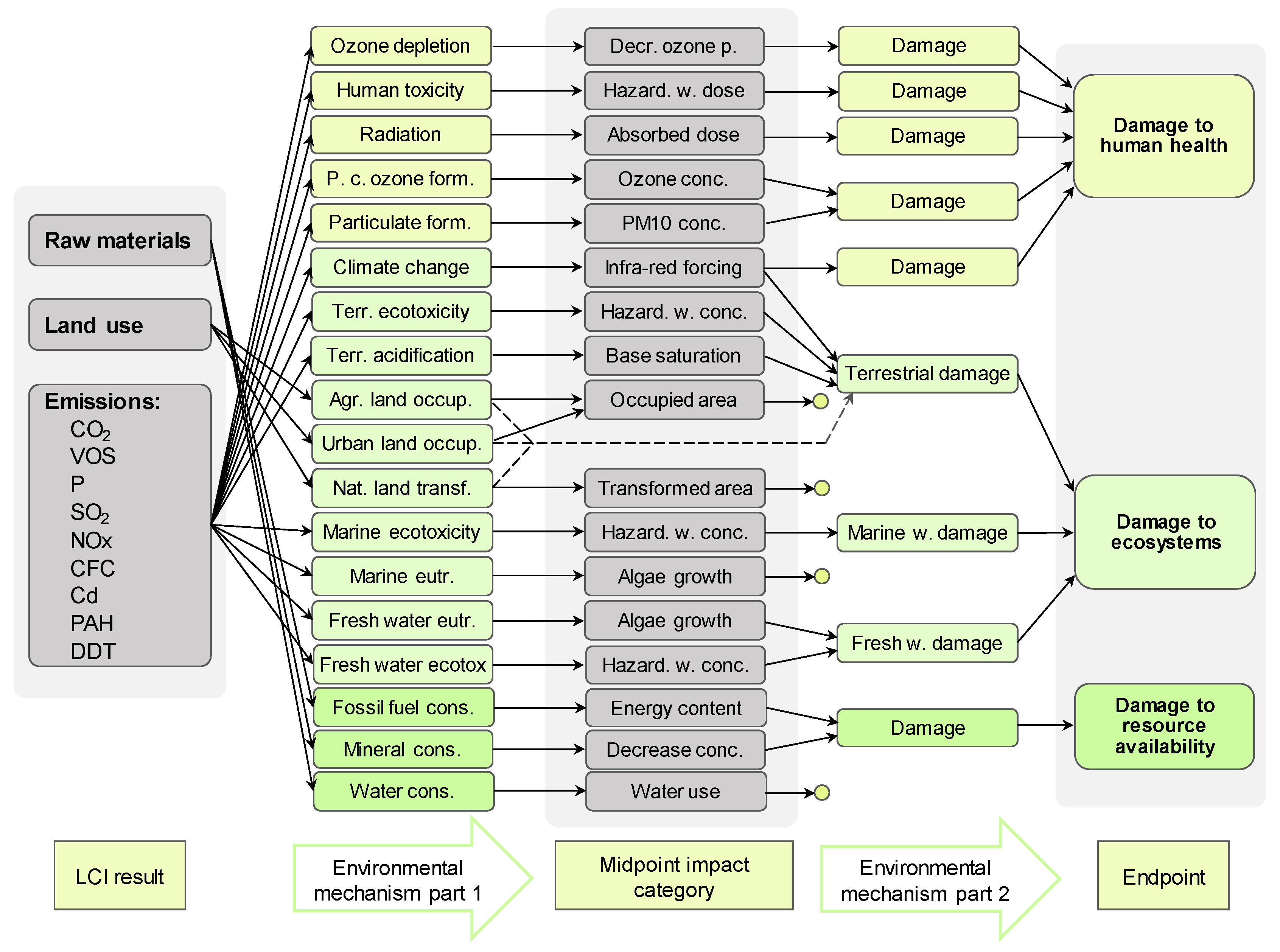
ReCiPe 2008 method has been selected in this study for the impact assessment stage [44]. This methodology comprises eighteen impact subcategories at the midpoint level, and these midpoint subcategories are transformed and combined into three endpoint categories: ecosystem quality, human health, and resource depletion. Figure 1 shows the relationships between LCI parameters, midpoint indicators and endpoint indicators according to RECIPE 2008.
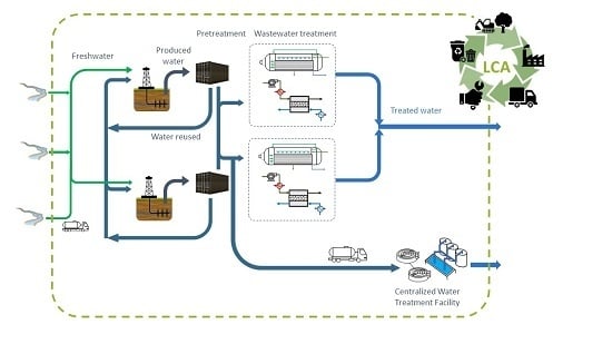
The functional unit used in this work is the extraction of 1 m3 of treated water for the comparison of wastewater treatment technologies, and 1 dam3 (1000 m3) of produced gas for the complete management model. The system boundary for the wastewater treatment in shale gas extraction includes freshwater consumption, the use of raw materials, energy and chemicals, wastewater treatment facilities, and final disposals of waste material, such as the sludge and brine.
2.1. Wastewater Treatment
2.1.1. Initial Wastewater Pre-treatment
A preliminary wastewater pretreatment has to be applied in order to prepare the wastewater for the selected desalination treatment or even for direct reuse on-site. There are some well-established treatment possibilities for the flowback water pretreatment, such as strainer filter, electrocoagulation, sedimentation, softening, etc.
The optimal pretreatment superstructure considered was obtained from the work by Carrero-Parreño et al. [49], where the optimal pretreatment arrangement is obtained depending on the input water properties and the desired destination of the wastewater. Our case study corresponds to the optimal pre-treatment solution for a desalination treatment by membrane or thermal technologies in order to remove TDS content. Thus, the first stage of the pretreatment is a strainer filter, whose main objective is to eliminate large particles and sludge from flowback water. Secondly, the electrocoagulation stage eliminates many species that the strainer filter cannot remove, avoiding the use of additional chemicals such as coagulants (Al2(SO4)3 or FeCl3, among others). Then, the flocs formed are removed in a sedimentation tank and the resultant water is sent to a softener tank, where the lime-soda process is used to soften the water. This process removes Mg2+ and Ca2+ precipitated as calcium carbonate and magnesium hydroxide. After that, the wastewater is sent to the corresponding desalination process to remove the TDS content. In any case, especially working with membrane technology, an additional filtration might be needed for the membrane preservation by the use of ultrafiltration or cartridge filters. The sludge produced in the sedimentation tank and in the softening process is dispatched to a filter press, allowing filtered water returns to the beginning of the pre-treatment plant for further treatment. The solid is handled as waste by an authorized manager.
2.1.2. Thermal-Based Technologies for the Wastewater Treatment
In this work, we have considered two thermal-based technologies of recent interest for the desalination process, based on the work by Onishi et al. [50], where a rigorous optimization model for the design of SEE/MEE systems that integrate MVR and heat recovery was introduced. The model was specially developed for the desalination of high salinity produced water from the shale gas industry. The advantage of this technology relies on the improvement of energy efficiency, while a high freshwater recovery ratio is obtained, and the brine disposal is reduced.
For the same ratio of recovery and water production, the MEE-MVR arrangement seems to be the best desalination alternative for shale produced water. The main reason lies in the fact that it is less expensive and versatile than the SEE-MVR arrangement [50]. In this case, the optimal system is composed of two evaporation effects.
The inventory data for the thermal-based technologies are given in Table 3.
2.1.3. Membrane Distillation Technology for the Wastewater Treatment
In this work, we have also considered a membrane-based technology from the work by Carrero-Parreño et al. [51], where an optimization model for the optimal design of a multistage membrane distillation system is presented to recover treated water and brine near to the Zero-Liquid Discharge (ZLD) condition. An optimal membrane configuration including 3 stages is considered. The inventory data for the membrane distillation technology is given in Table 4.
2.2. Wastewater Treatment Results
The environmental study was based on the LCA methodology, using ReCiPe Midpoint (H) and ReCiPe Endpoint (H, A) methods. These approaches allow the evaluation of several categories of environmental impact. Characterization factors at the midpoint level are focused on single environmental problems, while characterization factors at the endpoint level show the environmental impacts aggregated on three higher levels: human health, ecosystem quality and resource depletion [44]. Both approaches are complementary; the midpoint has a stronger relation to the environmental flows and has a lower uncertainty, while the endpoint shows an easier interpretation because it allows us to compare the indicators between them although it has a higher uncertainty [52].
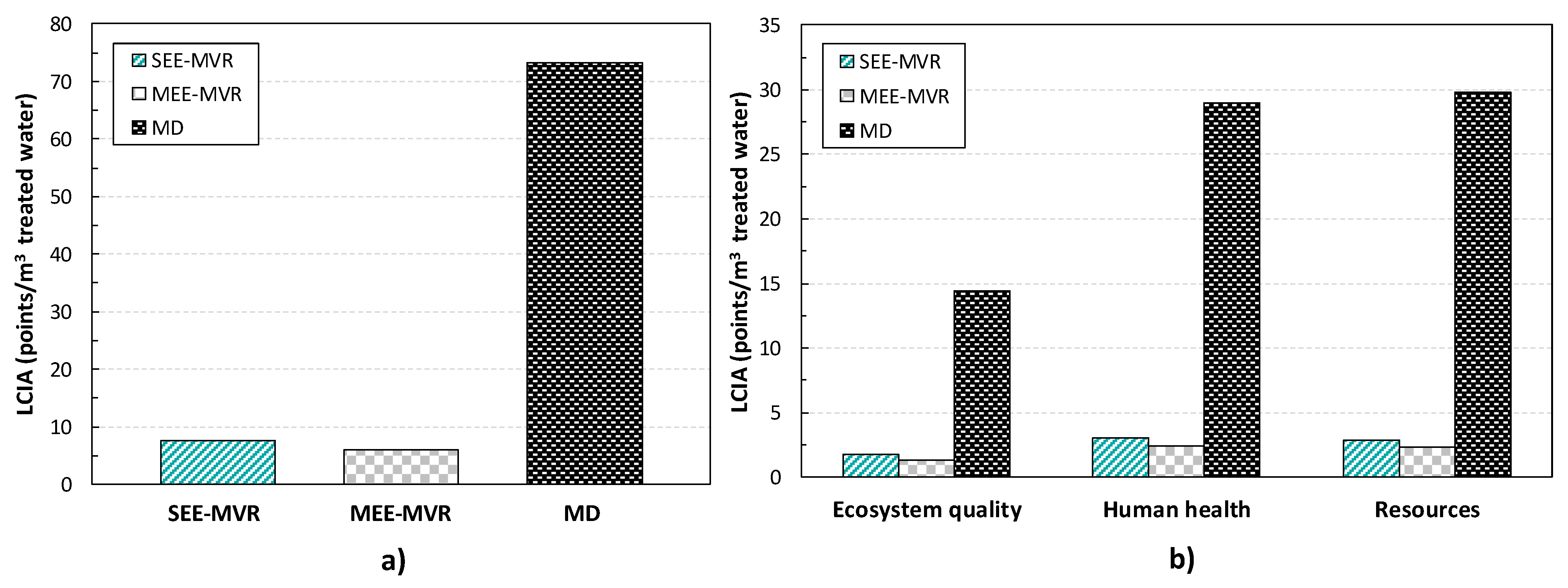
In order to compare the total environmental impact of the three technologies that are studied Figure 2 illustrates the behavior of the treatment alternatives according to the production of 1 m3 of treated water at the endpoint level, by using the hierarchical (H) perspective, based on the most usual policy principles, and the average (A) weighting. As can be seen, membrane technology has the highest environmental impact (in all damage categories). The total LCIA associated with the wastewater process reaches approximately 73.2 points/m3 of treated water using membrane technology and this impact reaches approximately 6.0 points/m3 treated water using MEE-MVR, which is around 91.8% lower. This result is due to the use of steam needed as the driving force in membrane distillation. From the environmental point of view, MEE-MVR has resulted to be the best alternative for the wastewater treatment in shale gas extraction because this technology uses less electricity than the SEE-MVR configuration (MEE-MVR has a total environmental impact 21.9% lower than SEE-MVR technology).
Additionally, in order to study the influence that each desalination technology has on the different subcategories, Figure 3 shows the contribution of each damage subcategory at the Endpoint (H, A) level in arbitrary units.
As can be observed, the most affected damage subcategories by the wastewater treatment processes are climate change followed by fossil depletion due to the use of electricity and steam in the case of membrane distillation, and due to the use of electricity in the case of evaporation technologies. This result is in concordance with previous studies, whose main focus was the estimation of GHG emissions associated with water management of the shale gas process [30,31,32,33].
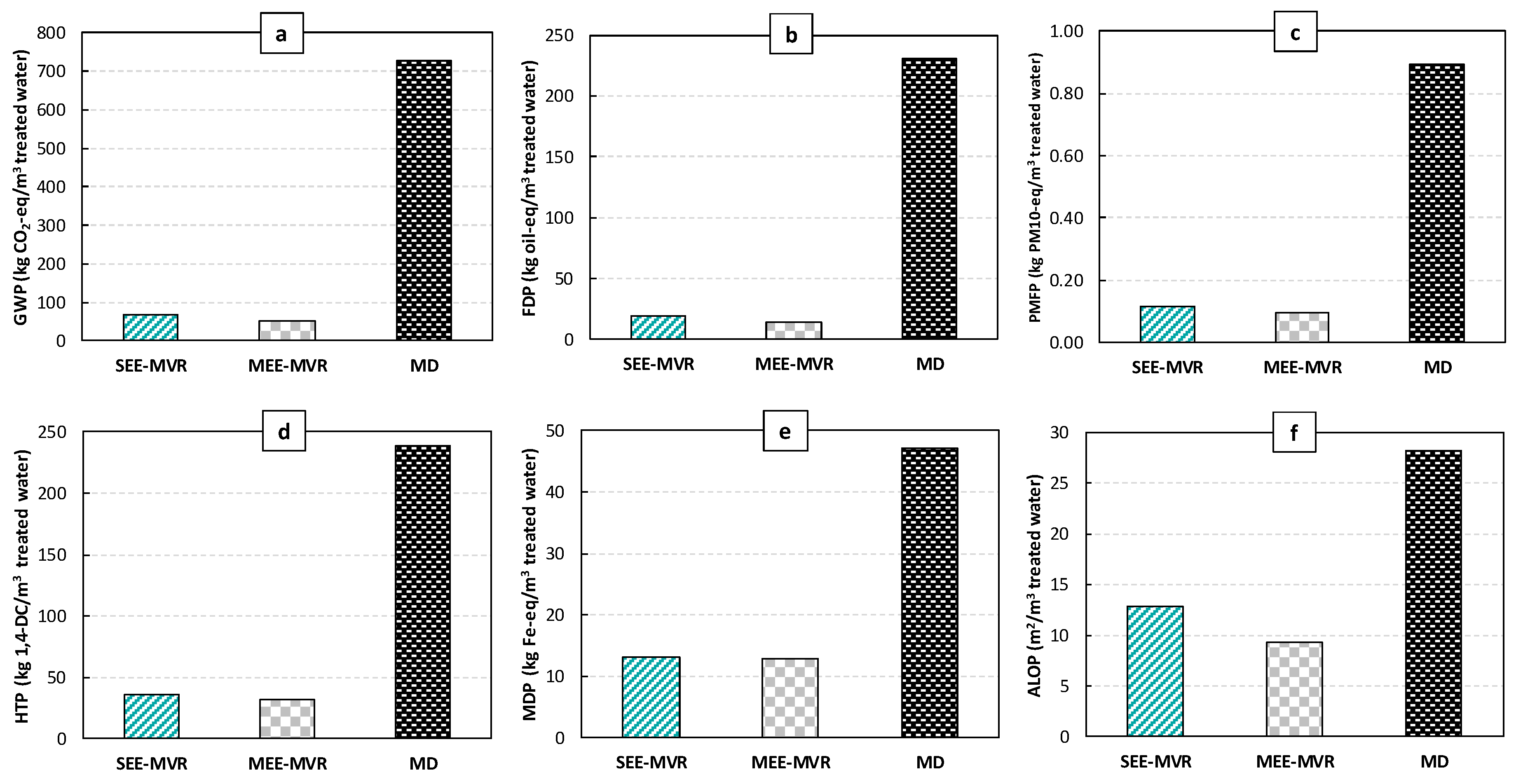
Although the rest of the subcategories are not really affected by wastewater treatments, the six more affected are shown in Figure 4 in their corresponding units at the Midpoint (H) level. The remaining figures for the eighteen ReCiPe damage subcategories are available in the Supplementary Material. For all the cases, membrane distillation has the highest impacts compared to thermal desalination technologies and, among them, MEE-MVR has lower impacts in all categories.
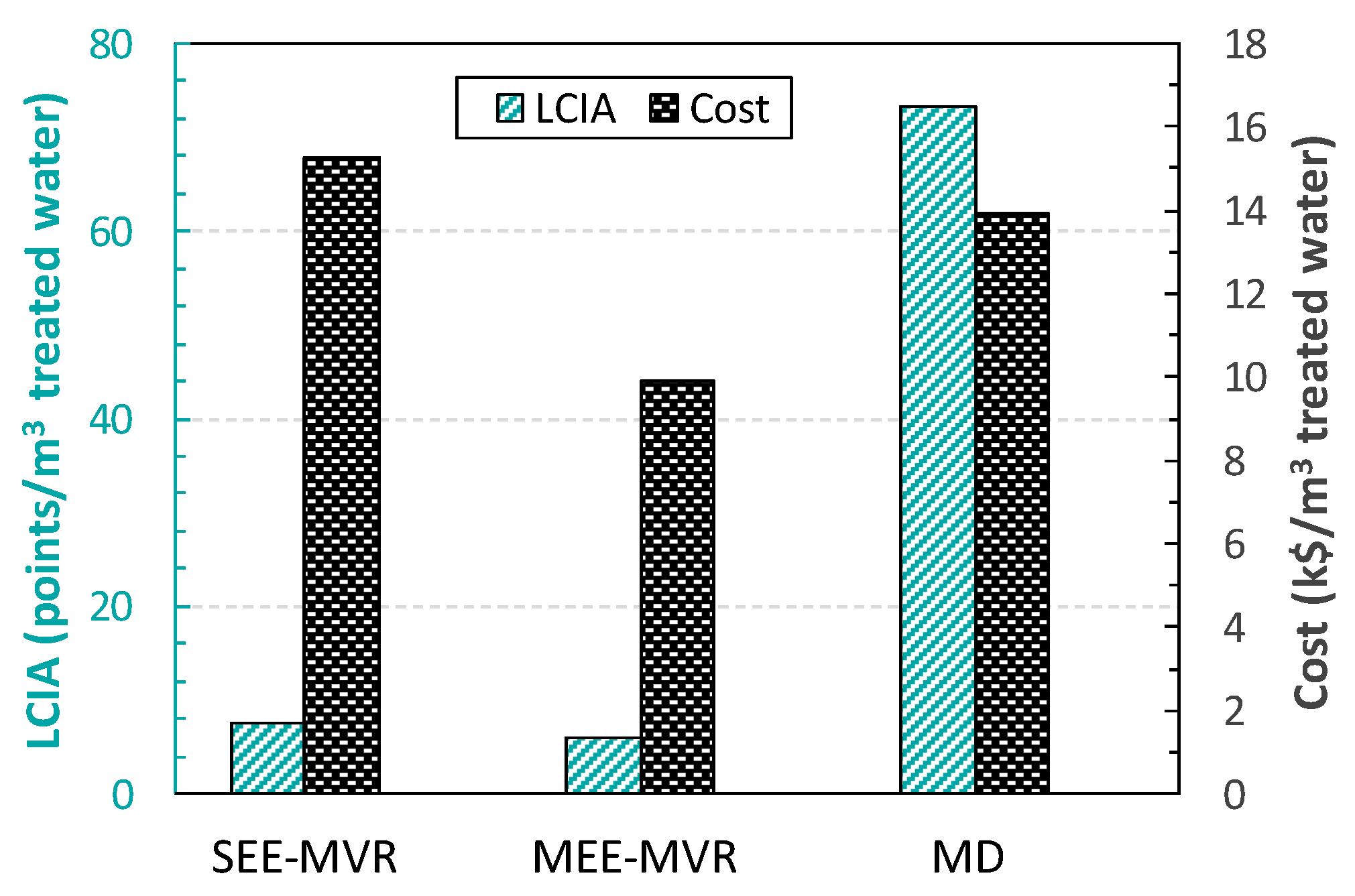
On the other hand, in order to evaluate the whole sustainability of the process, it is also interesting to compare the results obtained in our environmental study with other factors, such as the cost of each technology. In this sense, a comparison between the total impact and the cost of all the technologies (based on the works by Carrero-Parreño et al. [51] and Onishi et al. [50]) is shown in Figure 5.
The multiple-effect evaporation (MEE-MVR) system is around 35% less expensive than the SEE-MVR system, as was shown in the publication by Onishi et al. [50]. On the other hand, membrane distillation has a high cost due to the expensive cost of the steam used during the process. At the same time, MEE-MVR is the most environmentally friendly technology, which has a total environmental impact of around 91.8% lower than membrane distillation.
Another important aspect to consider is the amount of water recovered by each technology. In this way, a high rate of recovery should be obtained with the optimal configuration, while the brine removal should be near the zero-liquid discharge (ZLD) strategy [50,51]. Thermal desalination technologies allow recovering approximately 76.7% of water (regarding the inlet flow), while membrane distillation allows recovering approximately 33.5% of water.
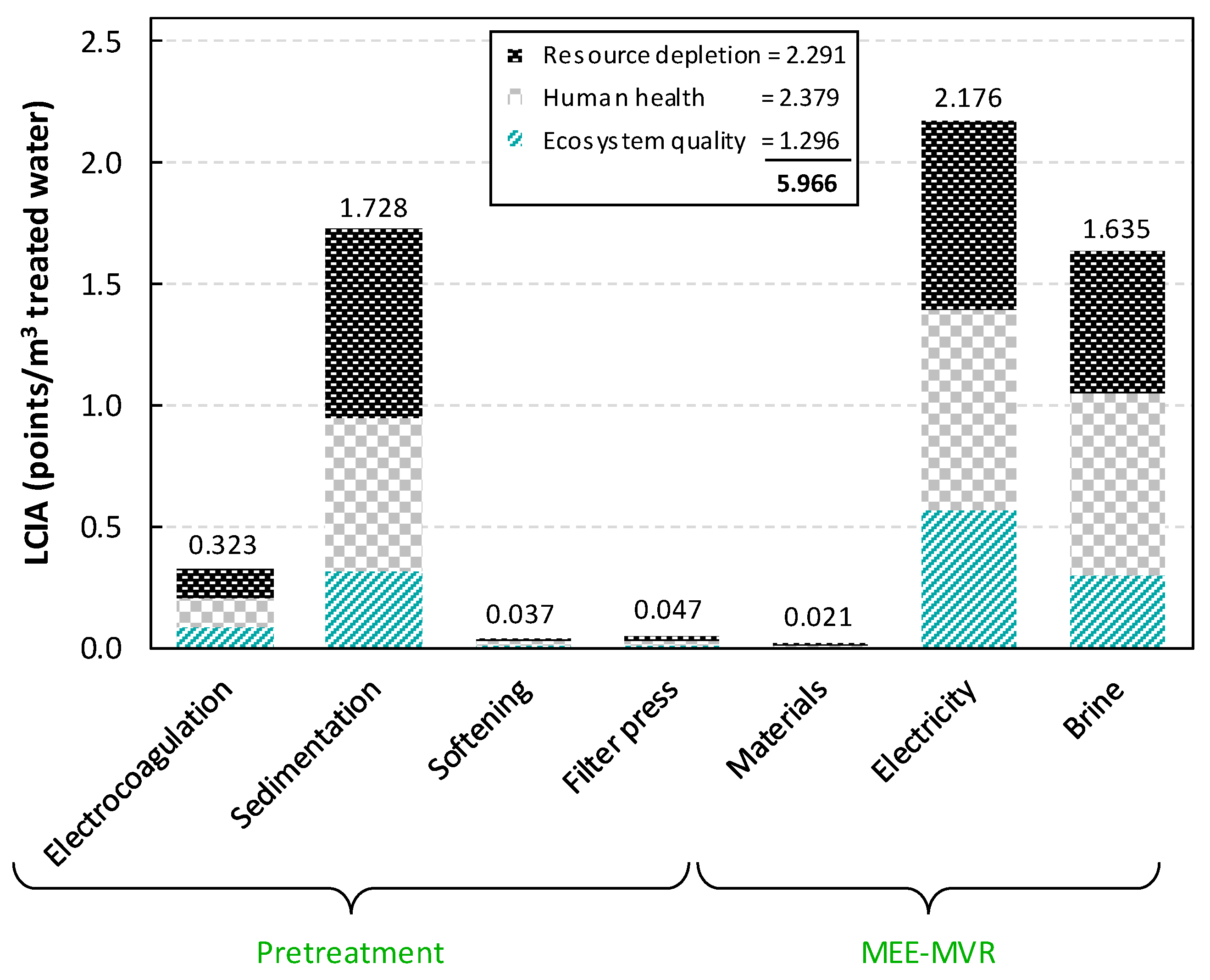
Due to the lower environmental impact, lower cost and higher water recovered; we can conclude that MEE-MVR is the most suitable technology for the wastewater treatment in shale gas extraction. For this reason, a more detailed study is presented for its optimal configuration. Figure 6 illustrates the environmental contributions of all the stages of the MEE-MVR treatment. Electricity used during the evaporation and the sedimentation stage is the factor that most influences the environmental impact, followed by brine discharge.
3. Economic vs. LCA of the Complete Water Management in Shale Gas Exploitation
In previous sections, we studied the pre-treatment and desalination stages related to flowback water in shale gas. However, to get a complete view of the relative importance of each one of the alternatives involved in shale gas exploitation, it is necessary to consider the whole supply chain, and simultaneously consider the cost and environmental impacts of all the alternatives involved in shale gas water management. To that end, we adapted the model proposed by Carrero Parreño et al. [53]. A brief description of the model capabilities is as follows:
A given company wants to fracture a set of wells distributed in different well pads (typically a well pad has between 6 and 20 wells) inside a period (i.e., one year). To that end, the company must decide, among a set of available freshwater sources, how much and when to acquire the water from each water source, and what quantity must be transported to each of the well pads. The water is then stored in freshwater tanks until it is used to frack the different wells in each well pad. The company must decide the optimal volume of each one of these tanks that will depend on the water availability and water demand in all the water-related activities. Once a well is fractured, there is a continuous flow of water (flowback water) that reaches the surface. This wastewater must be stored in appropriate tanks. Then this water can be sent to pre-treatment for posterior desalination in on-site facilities. It can be sent to a centralized water treatment facility, re-used in the fracture of other wells into the same well pad, or sent to other well pads of the same company with the objective of saving freshwater usage and reduce costs and environmental impacts.
The company should have data about the time to complete fracking operations, expected flow profile of flowback/produced water and gas release for each well as well as the gas prices. With that information, the company must decide the schedule of fracking activities in each well pad and coordinate all water flows. The model takes the form of a new Mixed-Integer Linear Programming (MILP) bi-criterion optimization model that addresses the profit maximization and the minimization Life Cycle Impact Assessment (LCIA) of water management in shale gas exploitation. A comprehensive description of the model is too large to be included here but a comprehensive description can be found in the Supplementary Material.
The following assumptions were made in the formulation of the model:
- A fixed time period is discretized into weeks as time intervals.
- Water transportation is only executed by trucks (the model can be easily extended to deal with transportation by pipes as well).
- The volume of water used to fracture a well must be available when needed—this includes the possibility of storage in tanks, or a ‘just in time water availability’—including water required in drilling, construction, and completion.
- The amount of water needed to carry out all the operations, as well as the variation in flowback water with time after the wells are turned in operation is known a priory.
- The well is turned in operation immediately after the drilled activities are finished.
- The amount of gas that releases and its variation with time after the wells are turned in operation are known a priori.
- Forecasts of gas prices for the complete time period are known a priori.
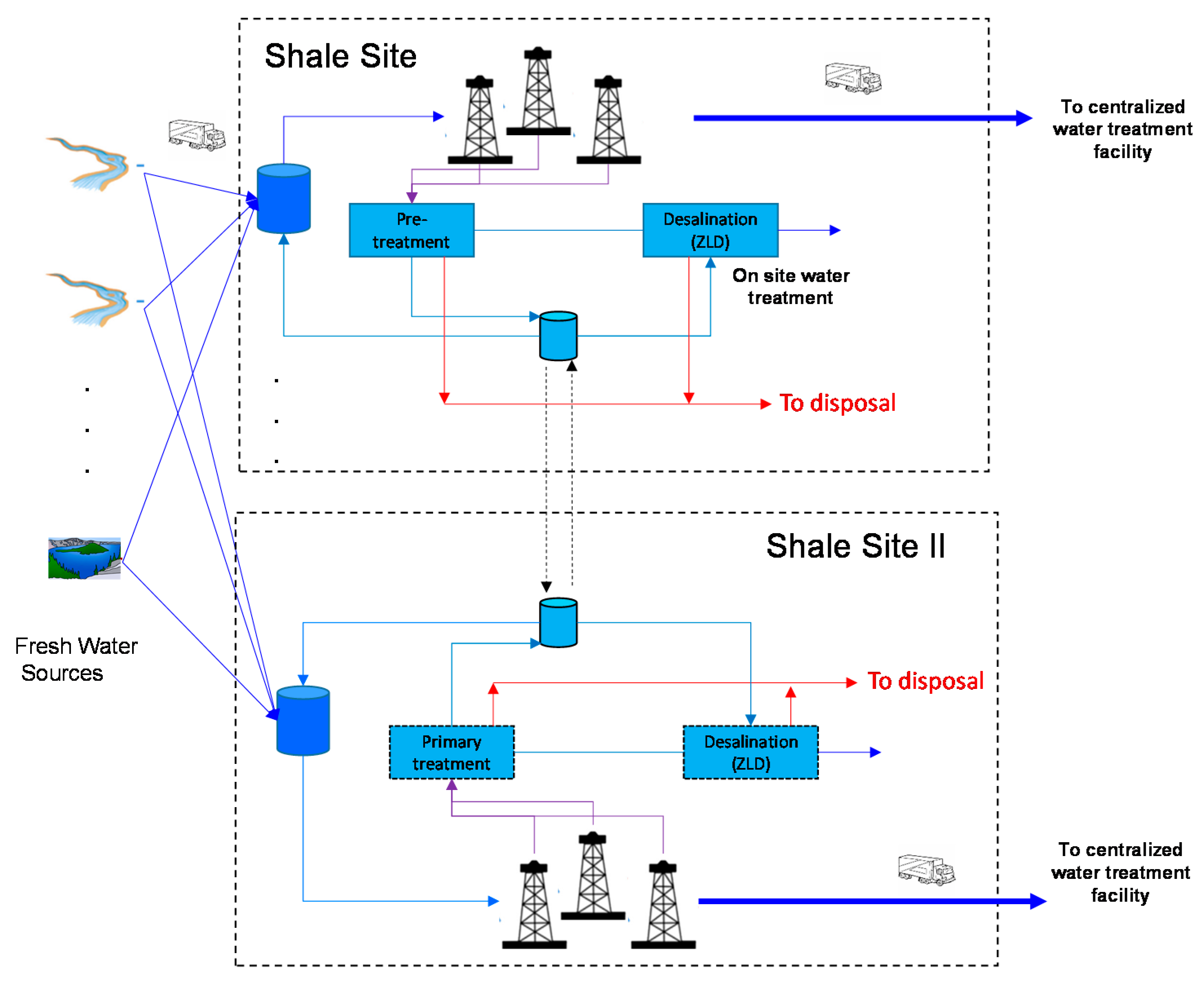
Figure 7 shows graphically a superstructure that includes all the alternatives commented.
For the environmental study, we follow the same approach as in the case of pre-treatment and desalination through the LCA methodology, using ReCiPe Midpoint (H) and ReCiPe Endpoint (H, A) methods. Data for LCIA inventory for water acquisition, freshwater and wastewater transport by trucks, etc. were obtained from the Ecoinvent database. v.3.4 and ReCiPe 2008 characterization factors. For the pre-treatment, we use the optimal configuration presented by Carrero-Parreño et al. [49] and the impact factors obtained in previous sections. For the on-site desalination, we use the MEE-MVR configuration that has proved to be the best alternative from both the economic and environmental points of view. Table 5, Table 6 and Table 7 show the midpoint indicator for transport, water extraction, disposal, pre-treatment and treatment used in the LCA. In this case, all the impacts will be presented by dam3 of produced gas.
Case Study
The case study selected represents a possible typical situation for a shale company. Data are based on average values for the Marcellus basin. In this example, the company has to manage four well pads separated from each other between 20 and 30 km. Therefore, the company considers that recycling water between the different well pads could be a profitable strategy to reduce freshwater consumption. The company identified three possible freshwater sources placed between 25 and 65 km from the different well pads. The four well pads have 6, 8, 7 and 6 wells respectively, and the company wants to fracture all of them within a period of 1 year. Based on their previous experience and knowledge of the basin characteristics, the company knows the water demand of each well, the expected variation with time of the flowback water, and the variation with time of gas release in each well. We assume that the company has a precise forecast of natural gas prices for the period considered.
The company is also interested in studying the possibility of installing on-site water treatment units in some (or all) well pads or send the water to a centralized water treatment facility (CWT).
The problem requires a large amount of data, and therefore for the sake of clarity, we present all data needed in the case study in the supplementary material.
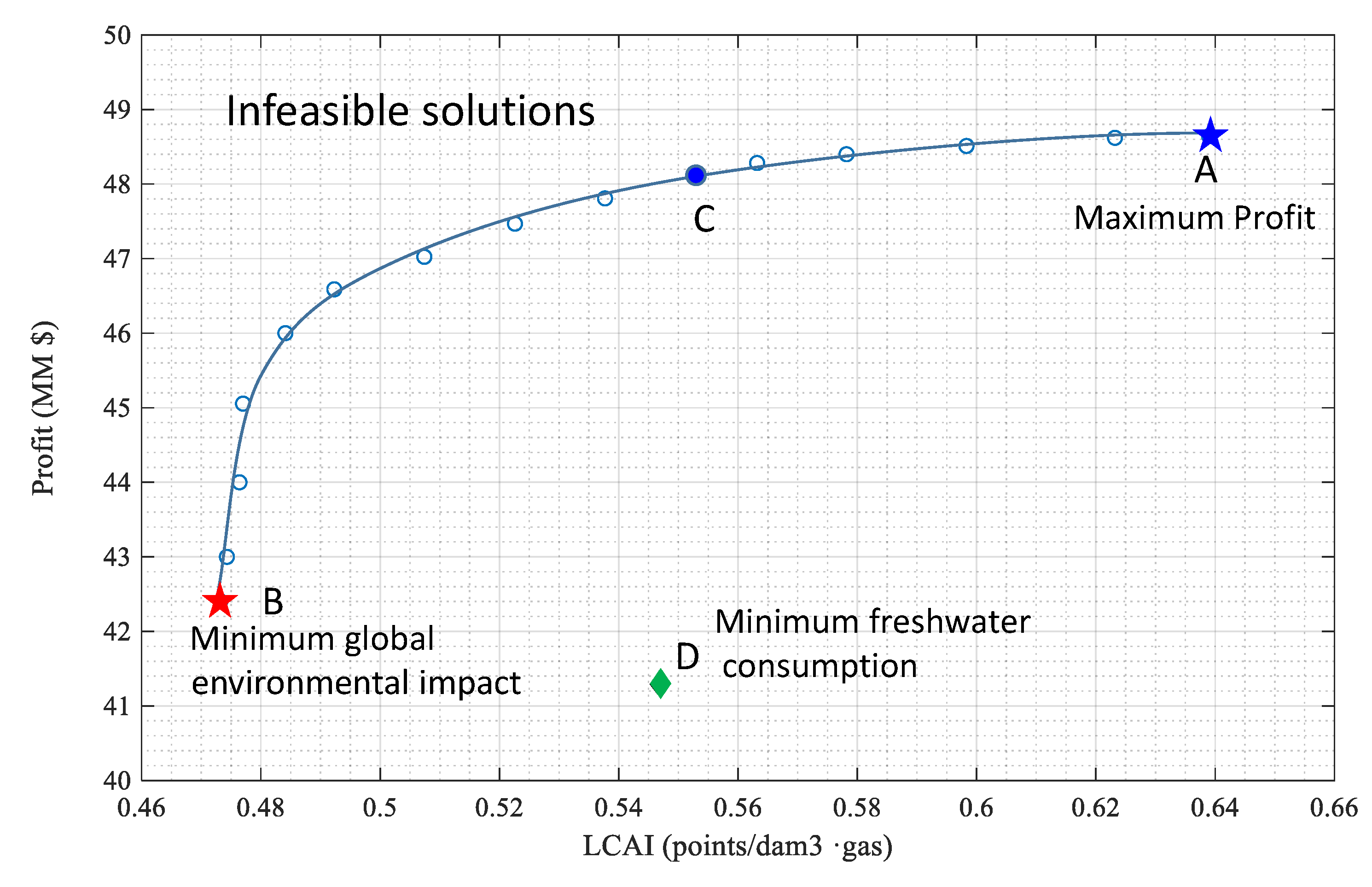
The resulting optimization model takes the form of a multi-objective mixed-integer linear programming problem (MO-MILP) in which we want to simultaneously maximize the profit and minimize the environmental impacts. In order to avoid the large dimensionality of dealing with all the mid-point categories, we focus our attention on the three end-point categories: Ecosystems Quality; Human Health; and Resources Depletion and the aggregated end-point. Initially, we consider a bi-objective optimization problem minimizing the aggregated end-point and maximizing the gross profit. Using the epsilon-constrained method [54,55] it is possible to generate the Pareto curve -shown in Figure 8 If for each of the points in the Pareto surface we calculate the individual contribution of the three end-point environmental impacts which shows that they are correlated (Table 8) Therefore, just considering the aggregated end-point is enough to capture all the trade-offs between maximizing the profit and minimizing the environmental impact.
The point A in Figure 8 corresponds to the maximum profit (MM $48.643) (MM stated for million of dollars) with an aggregated impact of 0.6390 points/dam3·gas. Point B in Figure 8 corresponds to the minimum environmental impact (0.4732 points/dam3·gas) that is a reduction in environmental impact around 25.9%, with a gross profit of MM $42.404 that corresponds to a reduction in profit of around 12.8%. This result coincides with the intuition that indicates that when we operate at the optimal conditions, we can only reduce the environmental impacts by reducing the benefits (or, of course, introducing some technological improvements). However, the most interesting part of the Pareto curve (Figure 8) is that there is a relatively large zone in which we can considerably reduce the environmental impacts with a minimum reduction in the profit. For example, if we decide to operate in point C in Figure 8, we can reduce the environmental impact by 13.5% with only 1.06% in the reduction of the gross profit.
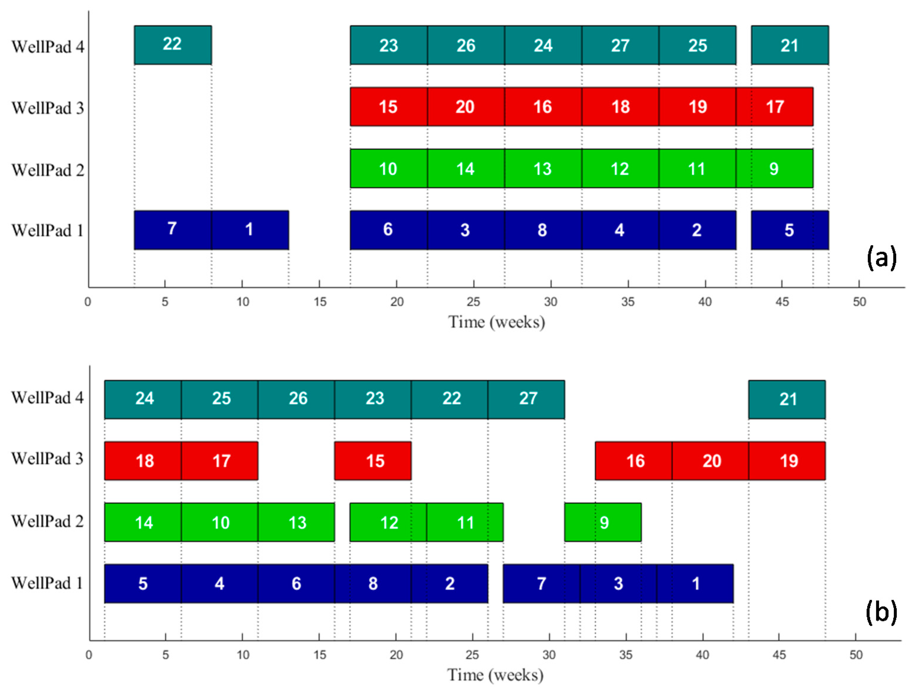
Figure 9 shows the optimal schedules for points A and B in Figure 8 (best economic and best environmental solutions). The schedule in the maximum profit solution tends to follow the gas prices to maximize the profit because the maximum gas production is just in the first two weeks after the well is turned in operation. However, it is worth to remark that gas prices forecasts have always some uncertainty. Therefore, good practice would be to operate, whenever possible, at a point in which the environmental impacts can be significantly reduced without scarifying too much the economic performance (e.g., point C in Figure 8)
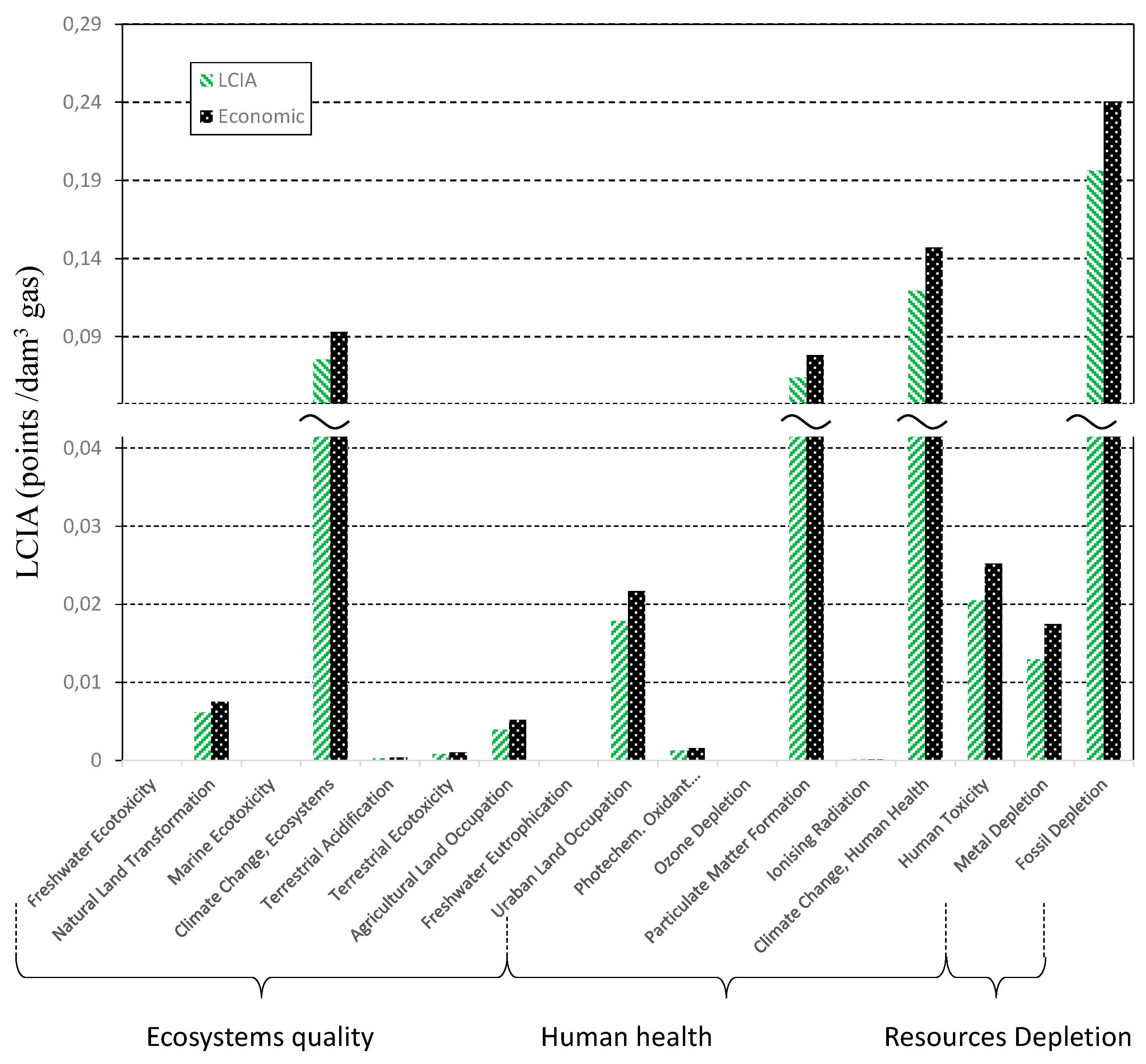
In Figure 10, we show a comparison of the main endpoint and mid-point indicators for the best solution from the environmental point of view and economic point of view. The most important impacts are due to fossil fuel depletion, climate change, and to a lesser extension land occupation and particulate matter formation.
Due to the large amount of data, a comprehensive summary of the results for the different scenarios (minimize the endpoint LCIA impact; maximize the profit and minimize freshwater consumption) can be found in the supplementary material.
One interesting result is that, although there is some correlation, minimizing the water footprint (e.g., minimizing freshwater consumption) it is not necessarily equivalent to minimizing the global environmental impacts. Point D in Figure 8 corresponds with the optimal solution when we minimize freshwater consumption. We get a very small reduction in freshwater consumption compared with the best environmental alternative but at the expense of significantly increasing the global environmental impacts. The reason is that the reduction in freshwater consumption is done by considerably increasing the water recycled between different well pads (62% more inter-well pad recycling) which have an important impact on transportation. Although the total water desalinated on-site is reduced (around 4%), it does not compensate for the increase in transport. Again, the decision is case dependent and we have to decide which is the relative importance of the water footprint versus other impacts (e.g., climate change). Saving freshwater could be much more important in water-scarce zones. In any case, the final decision must be based on each case data and models like the one used in this work are a tool to take informed decisions.
4. Conclusions
This paper studies the life cycle impact assessment of the wastewater treatment in the shale gas extraction, including the most common technologies for the pretreatment and three different desalination alternatives of recent interest, such as SEE-MVR, MEE-MVR, and Membrane Distillation. Thus, the life cycle analyses developed in this work might be a valuable aspect to make the best decisions on environmental aspects related to the wastewater treatment for the water reuse in shale gas exploitation.
The best option to desalinate water is using a thermal-based technology. It is shown that multiple-effect evaporation with mechanical vapor recompression (MEE-MVR) is the best alternative. Membrane distillation has a higher environmental impact than thermal technologies, but it could be competitive in some circumstances. For example, at distant shale gas extraction sites, the power supply might be limited or even not available, which makes MEE-MVR alternative an impractical choice because it needs a constant power supply. However, the MD alternative works with industrial steam, which might be easily obtained from waste heat recovered from the shale gas operations.
Obviously, the best choice to treat shale wastewater from an environmental point of view is the direct reuse, which might be given in the well pad itself or in other nearby well pads.
Electricity and brine discharge are the factors that most influence the environmental impacts in the optimal configuration (pretreatment + MEE-MVR).
The optimal gas production, and therefore the drilling schedule, tends to follow the gas prices forecast to maximize the profit. However, the multi-objective optimization shows that it is possible to obtain important reductions in environmental impacts with small variations in the profit. If we take into account that in the gas prices forecast there is always some uncertainty a good practice would be to operate at a point in which we can reduce the environmental impacts without sacrificing too much the economic benefit.
Minimizing water consumption is not necessarily the best environmental alternative, even though there is a correlation between environmental impacts and freshwater consumption. It is possible that a reduction in the water footprint (i.e., freshwater consumption) is at the expense of increasing inter-well pad recycling, increasing the impacts related to transport and consequently increasing the impact of other environmental indicators. Of course, the optimal trade-off is case dependent and the factors involved can only be treated through an optimization model that captures the most relevant factors in each case.
Supplementary Materials
The following are available online at https://0-www-mdpi-com.brum.beds.ac.uk/2071-1050/12/4/1686/s1.
- Comparison between thermal and membrane-based technologies for all the subcategories of impact using ReCiPe Midpoint (H).
- Waste Water Management: Comprehensive Mathematical Model Formulation.
- Case Study: Data and Results for the best environmental solution; best economic solution (maximum gross profit) and the best solution for minimum freshwater consumption.
Author Contributions
All the authors have significantly contributed to the article. The first draft manuscript was written by J.A.C. and reviewed by all the authors. J.A.L. and A.C.-P. develop all the models related to pre-treatment and Membrane Distillation Models. N.Q. developed the L.C.A. models and comparisons between technologies. The original Management model was developed by A.C.-P. and I.E.G. The final bi-criterion optimization model was written by J.A.C. and validated by I.E.G. All authors have read and agreed to the published version of the manuscript.
Funding
This project has received funding from the Spanish «Ministerio de Economía, Industria y Competitividad» under the projects CTQ2016-77968-C3-1-P and CTQ2016-77968-C3-2-P (FEDER, UE).
Conflicts of Interest
The authors declare no conflict of interests.
References
- International Energy Agency. Global Energy & CO2 Status Report—The Latest Trends in Energy and Emissions 2018.; IEA Publications: Paris, France, 2019. [Google Scholar]
- BP. BP Statistical Review of World Energy Statistical Review of World; Pureprint Group Limited: London, UK, 2019. [Google Scholar]
- Stevens, P. The ‘Shale Gas Revolution’: Developments and Changes; Chatham House: London, UK, 2012; pp. 2–3. [Google Scholar]
- U.S. Energy Information Administration. Annual Energy Outlook 2019 with Projections to 2050; U.S. Energy Information Administration: Washington, DC, USA, 2019; Volume January. [Google Scholar]
- Lira-Barragán, L.F.; Ponce-Ortega, J.M.; Guillén-Gosálbez, G.; El-Halwagi, M.M. Optimal Water Management under Uncertainty for Shale Gas Production. Ind. Eng. Chem. Res. 2016, 55, 1322–1335. [Google Scholar] [CrossRef]
- Nicot, J.-P.; Scanlon, B.R. Water use for shale gas production in Texas, U.S. U.S. Environ. Sci. Technol. 2012, 46, 3580–3586. [Google Scholar] [CrossRef] [PubMed]
- Stephenson, T.; Valle, J.E.; Riera-Palou, X. Modeling the relative GHG emissions of conventional and shale gas production. Environ. Sci. Technol. 2011, 45, 10757–10764. [Google Scholar] [CrossRef]
- Mauter, M.S.; Alvarez, P.J.J.; Burton, G.A.; Cafaro, D.C.; Chen, W.; Gregory, K.B.; Jiang, G.; Li, Q.; Pittock, J.; Reible, D.; et al. Regional Variation in Water Related Impacts of Shale Gas Development and Implications for Emerging International Plays. Environ. Sci. Technol. 2014, 48, 8298–8306. [Google Scholar] [CrossRef]
- Weber, C.L.; Clavin, C. Life cycle carbon footprint of shale gas: Review of evidence and implications. Environ. Sci. Technol. 2012, 46, 5688–5695. [Google Scholar] [CrossRef]
- Kuhn, M.; Umbach, F. Strategic Perspectives of Unconventional Gas: A Game Changer with Implications for the EU’s Energy Security; EUCERS: London, UK, 2011; Volume 1, ISBN 9780956903303. [Google Scholar]
- UNCTAD (United Nations Conference on Trade and Development). Commodities at a Glance: Special Issue on Shale Gas; UNCTAD: New York, NY, USA; Geneva, Switzerland, 2018. [Google Scholar]
- Bickle, M.; Goodman, D.; Mair, R.; Roberts, J.; Selley, R.; Shipton, Z.; Thomas, H.; Younger, P. Shale Gas Extraction in the UK: A Review of Hydraulic Fracturing; The Royal Academy of Engineering: London, UK, 2012; pp. 1–76. [Google Scholar]
- Vinson&Elkins. Shale Development in Denmark. Available online: http://fracking.velaw.com/shaledevelopment- (accessed on 6 June 2016).
- Martor, B. France: Evolutions in the Legal Framework for Shale Oil and Gas. Available online: http://www.shale-gas-information-platform.org/categories/legislation/expert-articles/martor-article.html (accessed on 8 July 2016).
- EPA. Technical Development Document for the Effluent Limitations Guidelines and Standards for the oil and Gas Extraction Point Source Category; Environmental Protection Agency: Washingtong, DC, USA, 2016. [Google Scholar]
- Hammond, G.P.; O’Grady, Á. Indicative energy technology assessment of UK shale gas extraction. Appl. Energy 2017, 185, 1907–1918. [Google Scholar] [CrossRef] [Green Version]
- Prpich, G.; Coulon, F.; Anthony, E.J. Review of the scientific evidence to support environmental risk assessment of shale gas development in the UK. Sci. Total Environ. 2016, 563, 731–740. [Google Scholar] [CrossRef]
- Lutz, B.D.; Lewis, A.N.; Doyle, M.W. Generation, transport, and disposal of wastewater associated with Marcellus Shale gas development. Water Resour. Res. 2013, 49, 647–656. [Google Scholar] [CrossRef]
- Gregory, K.B.; Vidic, R.D.; Dzombak, D.A. Water management challenges associated with the production of shale gas by hydraulic fracturing. Elements 2011, 7, 181–186. [Google Scholar] [CrossRef]
- Yang, L.; Grossmann, I.E.; Manno, J. Optimization models for shale gas water management. AIChE J. 2014, 60, 3490–3501. [Google Scholar] [CrossRef]
- Balaba, R.S.; Smart, R.B. Total arsenic and selenium analysis in Marcellus shale, high-salinity water, and hydrofracture flowback wastewater. Chemosphere 2012, 89, 1437–1442. [Google Scholar] [CrossRef] [PubMed]
- Chen, H.; Carter, K.E. Water usage for natural gas production through hydraulic fracturing in the United States from 2008 to 2014. J. Environ. Manage. 2016, 170, 152–159. [Google Scholar] [CrossRef] [PubMed]
- Estrada, J.M.; Bhamidimarri, R. A review of the issues and treatment options for wastewater from shale gas extraction by hydraulic fracturing. Fuel 2016, 182, 292–303. [Google Scholar] [CrossRef]
- Ellsworth, W.L. Injection-Induced Earthquakes. Science 2013, 341, 1225942. [Google Scholar] [CrossRef] [PubMed]
- Shaffer, D.L.; Arias Chavez, L.H.; Ben-Sasson, M.; Romero-Vargas Castrillón, S.; Yip, N.Y.; Elimelech, M. Desalination and Reuse of High-Salinity Shale Gas Produced Water: Drivers, Technologies, and Future Directions. Environ. Sci. Technol. 2013, 47, 9569–9583. [Google Scholar] [CrossRef]
- Michel, M.M.; Reczek, L. Pre-Treatment of Flowback Water To Desalination. Membr. Membr. Process. Environ. Prot. Monogr. Environ. Eng. Committee. Polish Acad. Sci. 2014, 119, 309–321. [Google Scholar]
- Coday, B.D.; Xu, P.; Beaudry, E.G.; Herron, J.; Lampi, K.; Hancock, N.T.; Cath, T.Y. The sweet spot of forward osmosis: Treatment of produced water, drilling wastewater, and other complex and difficult liquid streams. Desalination 2014, 333, 23–35. [Google Scholar] [CrossRef]
- Salcedo-Díaz, R.; Ruiz-Femenia, R.; Carrero-Parreño, A.; Onishi, V.C.; Reyes-Labarta, J.A.; Caballero, J.A. Combining Forward and Reverse Osmosis for Shale Gas Wastewater Treatment to Minimize Cost and Freshwater Consumption. In Computer Aided Chemical Engineering; Elsevier: Amsterdam, The Netherlands, 2017; Volume 40, pp. 2725–2730. [Google Scholar]
- Shaffer, D.L.; Werber, J.R.; Jaramillo, H.; Lin, S.; Elimelech, M. Forward osmosis: Where are we now? Desalination 2015, 356, 271–284. [Google Scholar] [CrossRef]
- Bartholomew, T.V.; Mauter, M.S. Multiobjective Optimization Model for Minimizing Cost and Environmental Impact in Shale Gas Water and Wastewater Management. ACS Sustain. Chem. Eng. 2016, 4, 3728–3735. [Google Scholar] [CrossRef]
- Jiang, M.; Hendrickson, C.T.; VanBriesen, J.M. Life Cycle Water Consumption and Wastewater Generation Impacts of a Marcellus Shale Gas Well. Environ. Sci. Technol. 2014, 48, 1911–1920. [Google Scholar] [CrossRef] [Green Version]
- Pekney, N.J.; Veloski, G.; Reeder, M.; Tamilia, J.; Rupp, E.; Wetzel, A. Measurement of atmospheric pollutants associated with oil and natural gas exploration and production activity in Pennsylvania’s Allegheny National Forest. J. Air Waste Manage. Assoc. 2014, 64, 1062–1072. [Google Scholar] [CrossRef] [PubMed]
- Coday, B.D.; Miller-Robbie, L.; Beaudry, E.G.; Munakata-Marr, J.; Cath, T.Y. Life cycle and economic assessments of engineered osmosis and osmotic dilution for desalination of Haynesville shale pit water. Desalination 2015, 369, 188–200. [Google Scholar] [CrossRef] [Green Version]
- Cooper, J.; Stamford, L.; Azapagic, A. Shale Gas: A Review of the Economic, Environmental, and Social Sustainability. Energy Technol. 2016, 4, 772–792. [Google Scholar] [CrossRef]
- Stamford, L.; Azapagic, A. Life cycle environmental impacts of UK shale gas. Appl. Energy 2014, 134, 506–518. [Google Scholar] [CrossRef]
- Tagliaferri, C.; Clift, R.; Lettieri, P.; Chapman, C. Shale gas: a life-cycle perspective for UK production. Int. J. Life Cycle Assess. 2017, 22, 919–937. [Google Scholar] [CrossRef] [Green Version]
- Gao, J.; You, F. Shale Gas Supply Chain Design and Operations toward Better Economic and Life Cycle Environmental Performance: MINLP Model and Global Optimization Algorithm. ACS Sustain. Chem. Eng. 2015, 3, 1282–1291. [Google Scholar] [CrossRef]
- Cafaro, D.C.; Grossmann, I.E. Strategic planning, design, and development of the shale gas supply chain network. AIChE J. 2014, 60, 2122–2142. [Google Scholar] [CrossRef]
- Carrero-Parreño, A.; Reyes-Labarta, J.A.; Salcedo-Díaz, R.; Ruiz-Femenia, R.; Onishi, V.C.; Caballero, J.A.; Grossmann, I.E. Holistic Planning Model for Sustainable Water Management in the Shale Gas Industry. Ind. Eng. Chem. Res. 2018, 57, 13131–13143. [Google Scholar] [CrossRef] [Green Version]
- Zhang, X.; Sun, A.Y.; Duncan, I.J. Shale gas wastewater management under uncertainty. J. Environ. Manage. 2016, 165, 188–198. [Google Scholar] [CrossRef]
- Burnham, A.; Han, J.; Clark, C.E.; Wang, M.; Dunn, J.B.; Palou-Rivera, I. Life-cycle greenhouse gas emissions of shale gas, natural gas, coal, and petroleum. Environ. Sci. Technol. 2012, 46, 619–627. [Google Scholar] [CrossRef]
- Laurenzi, I.J.; Jersey, G.R. Life cycle greenhouse gas emissions and freshwater consumption of marcellus shale gas. Environ. Sci. Technol. 2013, 47, 4896–4903. [Google Scholar] [CrossRef] [PubMed]
- Howarth, R.W.; Santoro, R.; Ingraffea, A. Methane and the greenhouse-gas footprint of natural gas from shale formations. Clim. Change 2011, 106, 679–690. [Google Scholar] [CrossRef] [Green Version]
- Goedkoop, M.; Heijungs, R.; Huijbregts, M.; De Schryver, A.; Struijs, J.; Zelm, R. Van ReCiPe 2008: A Life Cycle Impact Assessment Method which Comprises Harmonised Category Indicators at the Midpoint and the Endpoint Level; National Institute for Public Health and the Environment (RIVM): Biithoven, The Netherlands, 2009. [Google Scholar]
- Wernet, G.; Bauer, C.; Steubing, B.; Reinhard, J.; Moreno-Ruiz, E.; Weidema, B. The ecoinvent database version 3 (part I): Overview and methodology. Int. J. Life Cycle Assess. 2016, 21, 1218–1230. [Google Scholar] [CrossRef]
- ISO (International Organization for Standarization). ISO 14040:2006 Environmental Management—Life Cycle Assessment—Principles and Framework; ISO: Geneva, Switzerland, 2006. [Google Scholar]
- ISO (International Organization for Standarization). ISO 14044:2006 Environmental Management—Life Cycle Assessment—Requirements and Guidelines; ISO: Geneva, Switzerland, 2006. [Google Scholar]
- Rebitzer, G.; Ekvall, T.; Frischknecht, R.; Hunkeler, D.; Norris, G.; Rydberg, T.; Schmidt, W.-P.; Suh, S.; Weidema, B.P.; Pennington, D.W. Life cycle assessment: Part 1: Framework, goal and scope definition, inventory analysis, and applications. Environ. Int. 2004, 30, 701–720. [Google Scholar] [CrossRef] [PubMed]
- Carrero-Parreño, A.; Onishi, V.C.; Salcedo-Díaz, R.; Ruiz-Femenia, R.; Fraga, E.S.; Caballero, J.A.; Reyes-Labarta, J.A. Optimal Pretreatment System of Flowback Water from Shale Gas Production. Ind. Eng. Chem. Res. 2017, 56, 4386–4398. [Google Scholar] [CrossRef] [Green Version]
- Onishi, V.C.; Carrero-Parreño, A.; Reyes-Labarta, J.A.; Fraga, E.S.; Caballero, J.A. Desalination of shale gas produced water: A rigorous design approach for zero-liquid discharge evaporation systems. J. Clean. Prod. 2017, 140, 1399–1414. [Google Scholar] [CrossRef] [Green Version]
- Carrero-Parreño, A.; Onishi, V.C.; Ruiz-Femenia, R.; Salcedo-Díaz, R.; Caballero, J.A.; Reyes-Labarta, J.A. Optimization of multistage membrane distillation system for treating shale gas produced water. Desalination 2019, 460, 15–27. [Google Scholar] [CrossRef] [Green Version]
- Rosenbaum, R.K.; Hauschild, M.Z.; Boulay, A.M.; Fantke, P.; Laurent, A.; Núñez, M.; Vieira, M. Life Cycle Impact Assessment; Springer: Frankfurt, Germany; Cincinnati, OH, USA, 2017; ISBN 9783319564753. [Google Scholar]
- Carrero-Parreño, A.; Quirante, N.; Ruiz-Femenia, R.; Reyes-Labarta, J.A.; Salcedo-Díaz, R.; Grossmann, I.E.; Caballero, J.A. Economic and environmental strategic water management in the shale gas industry: Application of cooperative game theory. AIChE J. 2019, 65, 1–15. [Google Scholar] [CrossRef]
- Mavrotas, G.; Florios, K. An improved version of the augmented s-constraint method (AUGMECON2) for finding the exact pareto set in multi-objective integer programming problems. Appl. Math. Comput. 2013, 219, 9652–9669. [Google Scholar] [CrossRef]
- Mavrotas, G. Effective implementation of the ε-constraint method in Multi-Objective Mathematical Programming problems. Appl. Math. Comput. 2009, 213, 455–465. [Google Scholar] [CrossRef]
Figure 1.
Relationship between Life Cycle Impact (LCI) parameters (left), midpoint indicator (middle), and endpoint indicator (right) in ReCiPe 2008. (Abbreviations: p.c. ozone form = photochemical ozone formation; form = formation; Terr = terrestrial; Agr = Agricultural; Nat = Natural; eutr. = Etutrophication; Hazard w. dose = Hazard weighted dose; Hazard w. conc = Hazard weighted concentration; PM10 = particles lower than 10 µm; Fresh w. damage = Fresh water damage; Marine w damage = Marine water damage).

Figure 2.
Comparison of the environmental impact of the three technologies. (a) Total Life Cycle Impact Assessment (LCIA) using ReCiPe Endpoint (H, A). (b) LCIA of the main damage categories using ReCiPe Endpoint (H, A). (SEE-MVR = Single Effect Evaporation with Mechanical Vapor Recompression; MEE-MVR = Multiple Effect Evaporation with Mechanical Vapor Recompression; MD = Membrane Distillation).

Figure 3.
Comparison of the environmental impact subcategories using ReCiPe Endpoint (H, A).

Figure 4.
Environmental impact subcategories most affected by wastewater treatment: (a) Global warming potential (GWP), (b) Fossil depletion potential (FDP), (c) Particulate matter formation potential (PMFP), (d) Human toxicity potential (HTP), (e) Metal depletion potential (MDP), and (f) Agricultural land occupation potential (ALOP).

Figure 5.
Comparison of the environmental impact subcategories.

Figure 6.
Environmental impact contributions of all the wastewater treatment stages in the optimal alternative (pretreatment + MEE-MVR) using ReCiPe Endpoint (H, A).
Figure 6.
Environmental impact contributions of all the wastewater treatment stages in the optimal alternative (pretreatment + MEE-MVR) using ReCiPe Endpoint (H, A).

Figure 7.
Superstructure of alternatives for the water management model. It includes different freshwater sources, a variable number of wells in each well pad, freshwater tank(s), flowback water pre-treatment and desalination, wastewater storage, inter- and intra-well pad(s) recycling, centralized water treatment facilities, and disposal sites.

Figure 8.
Pareto curve for the minimization of the global LCIA environmental impact and maximization of the gross profit. The point A is the maximum profit, B is the minimum global environmental impact. Point C is a point in which the profit decreases only 1.06% while the environmental impact decreases in 13.5%. Point D is the optimal solution when we minimize freshwater consumption.

Figure 9.
Gantt Chart for the Optimal fracking schedule. (a) Maximum profit. (b) Minimum environmental impact. The number in each rectangle is the identification of individual wells in each well pad.
Figure 9.
Gantt Chart for the Optimal fracking schedule. (a) Maximum profit. (b) Minimum environmental impact. The number in each rectangle is the identification of individual wells in each well pad.

Figure 10.
Comparison of the environmental impact subcategories using ReCiPe Endpoint (H, A) for the optimal solution for the best economic and environmental solutions (points A and B in Figure 9).
Figure 10.
Comparison of the environmental impact subcategories using ReCiPe Endpoint (H, A) for the optimal solution for the best economic and environmental solutions (points A and B in Figure 9).


Table 1.
Inventory data for wastewater pretreatment. (Functional unit: m3 treated water).
| Parameter | Quantity | Units | Ecoinvent Input |
|---|---|---|---|
| Pretreatment plant * | |||
| Inlet flow | 1.001 | m3/m3 treated water | |
| Outlet flow | 1.000 | m3/m3 treated water | |
| Electrocoagulation | |||
| -Material-HDPE (Hihg density polyethylene) | 1.616 × 10⁻⁴ | kg/m3 treated water | [GLO] market for polyethylene, high density |
| -Electricity | 4.336 | kWh/m3 treated water | [GB] market for electricity, high voltage |
| Sedimentation | |||
| -Electricity | 8.599 × 10⁻³ | kWh/m3 treated water | [GB] market for electricity, high voltage |
| -Steel | 8.799 × 10⁻⁴ | kg/m3 treated water | [GLO] market for steel, chromium steel 18/8 |
| -HDPE | 5.799 × 10⁻⁶ | kg/m3 treated water | [GLO] market for polyethylene, high density |
| -Concrete | 9.999 × 10⁻⁶ | m3/m3 treated water | [RoW] concrete production, for civil engineering, with cement CEM II/B |
| Softening | |||
| -Material-Fiberglass | 4.483 × 10⁻⁴ | kg/m3 treated water | [GLO] market for glass fiber reinforced plastic, polyamide, injection molded |
| -Lime | 0.199 | kg/m3 treated water | [GLO] market for lime |
| -Soda | 0.570 | kg/m3 treated water | [GLO] market for soda ash, light, crystalline, heptahydrate |
| Filter press | |||
| -Sludge inlet | 1.218 | kg/m3 treated water | [RoW] drying, sewage sludge |
| -Sludge outlet | 0.616 | kg/m3 treated water | [GLO] market for sewage sludge, dried |
| -Material-Polypropylene | 4.320 × 10⁻⁵ | kg/m3 treated water | [GLO] market for polypropylene, granulate |
| -Electricity | 0.566 | kWh/m3 treated water | [GB] market for electricity, high voltage |
* Source: Carrero-Parreño et al. [49].
Table 2.
Inventory data for the potential emissions outputs of wastewater pre-treatment.
| Parameter | Quantity | Units |
|---|---|---|
| Pretreatment plant | ||
| Emissions | ||
| -Sand (silica, quartz) | 66.258 | kg/m3 treated water |
| -Hydrochloric acid | 1.469 | kg/m3 treated water |
| -Petroleum distillate | 0.367 | kg/m3 treated water |
| -Isopropanol | 0.367 | kg/m3 treated water |
| -Potassium chloride | 0.245 | kg/m3 treated water |
| -Hydroxyethyl cellulose | 0.245 | kg/m3 treated water |
| -Ethylene glycol | 0.184 | kg/m3 treated water |
| -Sodium potassium hydroxide | 4.898 × 10⁻² | kg/m3 treated water |
| -Ammonium persulfate | 4.898 × 10⁻² | kg/m3 treated water |
| -Borate salts | 4.898 × 10⁻² | kg/m3 treated water |
| -Citric acid | 1.837 × 10⁻² | kg/m3 treated water |
| -Glutaraldehyde | 4.898 × 10−-3 | kg/m3 treated water |
| -Formamide | 4.898 × 10⁻³ | kg/m3 treated water |
| -Diesel | 9.304 | kg/m3 treated water |
| -Polyacrylamide | 0.556 | kg/m3 treated water |
| -Sodium chloride | 5.831 × 10⁻⁵ | kg/m3 treated water |
Table 3.
Inventory data for thermal-based technologies. (Functional unit: m3 treated water).
| Parameter | Quantity | Units | Ecoinvent input |
|---|---|---|---|
| Single-Effect Evaporation with Mechanical Vapor Recompression (SEE-MVR) * | |||
| Feedwater | 1.304 | kg/s | |
| Nickel amount | 4.585 × 10⁻³ | kg/m3 treated water | [GLO] market for nickel, 99.5% |
| Chromium steel amount | 5.047 × 10⁻³ | kg/m3 treated water | [GLO] market for steel, chromium steel 18/8 |
| Electricity | 51.496 | kWh/m3 treated water | [GB] market for electricity, high voltage |
| Brine | 93.064 | kg/m3 treated water | [RER] sodium chloride production, brine solution |
| Treated water | 1.000 | m3/m3 treated water | |
| Multiple-Effect Evaporation with Mechanical Vapor Recompression (MEE-MVR) * | |||
| Feedwater | 1.304 | kg/s | |
| Nickel amount | 3.212 × 10⁻³ | kg/m3 treated water | [GLO] market for nickel, 99.5% |
| Chromium steel amount | 1.385 × 10⁻³ | kg/m3 treated water | [GLO] market for steel, chromium steel 18/8 |
| Electricity | 29.188 | kWh/m3 treated water | [GB] market for electricity, high voltage |
| Brine | 93.064 | kg/m3 treated water | [RER] sodium chloride production, brine solution |
| Treated water | 1.000 | m3/m3 treated water | |
* Source: Onishi et al. [50].
Table 4.
Inventory data for membrane distillation technology. (Functional unit: m3 treated water).
| Parameter | Quantity | Units | Ecoinvent Input |
|---|---|---|---|
| Membrane technology * | |||
| Feedwater | 2.985 | m3/m3 treated water | |
| Electricity | 8.310 | kWh/m3 treated water | [GB] market for electricity, high voltage |
| Cooling water | 1.204 × 10⁵ | kg/m3 treated water | [Europe without Switzerland] market for tap water |
| Steam | 1.847 × 10³ | kg/m3 treated water | [GLO] market for steam, in the chemical industry |
| Membrane composition | |||
| -PTFE | 1.025 × 10⁻³ | kg/m3 treated water | [GLO] market for polypropylene, granulate |
| -PP | 1.377 × 10⁻² | kg/m3 treated water | [GLO] market for tetrafluoroethylene |
| Brine | 607.433 | kg/m3 treated water | [RER] sodium chloride production, brine solution |
| Treated water | 1.000 | m3/m3 treated water | |
* Source: Carrero-Parreño et al. (2017a).
Table 5.
ReCiPe Endpoint (H, A) indicator of ecosystem quality.
| Ecosystem Quality | ||||||||||
|---|---|---|---|---|---|---|---|---|---|---|
| Units | Freshwater Ecotoxicity | Natural Land Transformation | Marine Ecotoxicity | Climate Change | Terrestrial Acidification | Terrestrial Ecotoxicity | Agricultural Land Occupation | Freshwater Eutrophication | Urban Land Occupation | |
| Transport | points/T·km | 4.197 × 10⁻⁷ | 1.416 × 10⁻⁴ | 2.170 × 10⁻⁷ | 1.597 × 10⁻³ | 6.217 × 10⁻⁶ | 1.951 × 10⁻⁵ | 4.405 × 10⁻⁵ | 6.753 × 10⁻⁷ | 4.131 × 10⁻⁴ |
| Water extraction | points/kg | 4.876 × 10⁻⁹ | 7.197 × 10⁻⁸ | 9.823 × 10⁻¹⁰ | 3.247 × 10⁻⁶ | 1.049 × 10⁻⁸ | 2.851 × 10⁻⁹ | 7.656 × 10⁻⁷ | 1.785 × 10⁻⁸ | 8.810 × 10⁻⁸ |
| Disposal | points/kg | 6.248 × 10⁻⁶ | 0.000 | 2.532 × 10⁻⁷ | 0.000 | 0.000 | 1.374 × 10⁻⁵ | 0.000 | 0.000 | 0.000 |
| Pretreatment | points/kg | 7.045 × 10⁻⁷ | 4.649 × 10⁻⁶ | 1.490 × 10⁻⁷ | 3.104 × 10⁻⁴ | 9.500 × 10⁻⁷ | 3.357 × 10⁻⁷ | 8.978 × 10⁻⁵ | 7.351 × 10⁻⁷ | 8.831 × 10⁻⁶ |
| Treatment | points/kg | 5.748 × 10⁻⁷ | 9.257 × 10⁻⁶ | 1.249 × 10⁻⁷ | 4.390 × 10⁻⁴ | 1.646 × 10⁻⁶ | 5.473 × 10⁻⁷ | 1.892 × 10⁻⁴ | 1.441 × 10⁻⁶ | 1.462 × 10⁻⁵ |
Table 6.
ReCiPe Endpoint (H, A) indicator of human health.
| Human Health | |||||||
|---|---|---|---|---|---|---|---|
| Units | Photochemical Oxidant Formation | Ozone Depletion | Particulate Matter Formation | Ionizing Radiation | Climate Change | Human Toxicity | |
| Transport | points/T·km | 2.705 × 10⁻⁵ | 9.087 × 10⁻⁷ | 1.385 × 10⁻³ | 2.400 × 10⁻⁶ | 2.527 × 10⁻³ | 4.319 × 10⁻⁴ |
| Water extraction | points/kg | 2.687 × 10⁻⁸ | 7.558 × 10⁻¹⁰ | 1.507 × 10⁻⁶ | 3.010 × 10⁻⁸ | 5.137 × 10⁻⁶ | 1.698 × 10⁻⁶ |
| Disposal | points/kg | 0.000 | 0.000 | 0.000 | 1.580 × 10⁻⁸ | 0.000 | 5.524 × 10⁻⁴ |
| Pretreatment | points/kg | 6.333 × 10⁻⁶ | 3.377 × 10⁻⁸ | 2.002 × 10⁻⁴ | 3.445 × 10⁻⁷ | 4.911 × 10⁻⁴ | 7.862 × 10⁻⁵ |
| Treatment | points/kg | 5.911 × 10⁻⁶ | 6.604 × 10⁻⁸ | 2.283 × 10⁻⁴ | 9.430 × 10⁻⁷ | 6.945 × 10⁻⁴ | 2.670 × 10⁻⁴ |
Table 7.
ReCiPe Endpoint (H, A) indicator of resource depletion.
| Resource Depletion | |||
|---|---|---|---|
| Units | Metal Depletion | Fossil Depletion | |
| Transport | points/T·km | 1.195 × 10⁻⁴ | 4.300 × 10⁻³ |
| Water extraction | points/kg | 1.902 × 10⁻⁷ | 6.173 × 10⁻⁶ |
| Disposal | points/kg | 0.000 | 0.000 |
| Pretreatment | points/kg | 3.707 × 10⁻⁴ | 5.397 × 10⁻⁴ |
| Treatment | points/kg | 1.664 × 10⁻⁴ | 8.621 × 10⁻⁴ |
Table 8.
Optimal points on the Pareto curve for the simultaneous maximization of profit and minimization of the aggregated LCIA endpoint impact. Individual values of the three endpoint categories (Ecosystem Quality, Human Health and Resources Depletion) are also provided.
Table 8.
Optimal points on the Pareto curve for the simultaneous maximization of profit and minimization of the aggregated LCIA endpoint impact. Individual values of the three endpoint categories (Ecosystem Quality, Human Health and Resources Depletion) are also provided.
| Profit (k$) | Ecosystem Quality (points/dam3) | Human Health (points/dam3) | Resources Depletion (points/dam3) | Aggregated End-Point (points/dam3) | FreshWater Consumption (m3) |
|---|---|---|---|---|---|
| 48,643.0 | 0.1288 | 0.2522 | 0.2580 | 0.6390 | 178,893.8 |
| 48,620.0 | 0.1257 | 0.2459 | 0.2517 | 0.6232 | 178,893.8 |
| 48,510.7 | 0.1206 | 0.2360 | 0.2417 | 0.5983 | 178,893.8 |
| 48,400.1 | 0.1166 | 0.2282 | 0.2334 | 0.5782 | 167,470.0 |
| 48,282.6 | 0.1135 | 0.2222 | 0.2274 | 0.5632 | 167,470.0 |
| 48,129.5 | 0.1115 | 0.2182 | 0.2233 | 0.5529 | 164,989.5 |
| 47,807.7 | 0.1084 | 0.2122 | 0.2170 | 0.5377 | 157,453.7 |
| 47,468.1 | 0.1054 | 0.2063 | 0.2110 | 0.5226 | 155,745.1 |
| 47,024.1 | 0.1023 | 0.2003 | 0.2048 | 0.5074 | 149,376.2 |
| 46,588.4 | 0.0993 | 0.1944 | 0.1987 | 0.4923 | 146,314.2 |
| 46,000.0 | 0.0972 | 0.1913 | 0.1956 | 0.4841 | 144,920.0 |
| 45,055.0 | 0.0962 | 0.1883 | 0.1925 | 0.4770 | 141,947.8 |
| 44,000.0 | 0.0961 | 0.1881 | 0.1923 | 0.4764 | 141,882.5 |
| 43,000.0 | 0.0956 | 0.1873 | 0.1914 | 0.4743 | 141,105.5 |
| 42,404.0 | 0.0954 | 0.1870 | 0.1908 | 0.4732 | 139,713.6 |
© 2020 by the authors. Licensee MDPI, Basel, Switzerland. This article is an open access article distributed under the terms and conditions of the Creative Commons Attribution (CC BY) license (http://creativecommons.org/licenses/by/4.0/).
Share and Cite
MDPI and ACS Style
Caballero, J.A.; Labarta, J.A.; Quirante, N.; Carrero-Parreño, A.; Grossmann, I.E. Environmental and Economic Water Management in Shale Gas Extraction. Sustainability 2020, 12, 1686. https://0-doi-org.brum.beds.ac.uk/10.3390/su12041686
AMA Style
Caballero JA, Labarta JA, Quirante N, Carrero-Parreño A, Grossmann IE. Environmental and Economic Water Management in Shale Gas Extraction. Sustainability. 2020; 12(4):1686. https://0-doi-org.brum.beds.ac.uk/10.3390/su12041686
Chicago/Turabian StyleCaballero, José A., Juan A. Labarta, Natalia Quirante, Alba Carrero-Parreño, and Ignacio E. Grossmann. 2020. "Environmental and Economic Water Management in Shale Gas Extraction" Sustainability 12, no. 4: 1686. https://0-doi-org.brum.beds.ac.uk/10.3390/su12041686
Note that from the first issue of 2016, this journal uses article numbers instead of page numbers. See further details here.