A Bicycle Origin–Destination Matrix Estimation Based on a Two-Stage Procedure

Korea Institute Science Technology Information, Dajeon 34141, Korea
Sustainability 2020, 12(7), 2951; https://0-doi-org.brum.beds.ac.uk/10.3390/su12072951
Submission received: 25 February 2020
/
Revised: 30 March 2020
/
Accepted: 3 April 2020
/
Published: 7 April 2020
(This article belongs to the Collection Bicycling Today: Establishing and Learning from the State of the Art)
Abstract
:As more people choose to travel by bicycle, transportation planners are beginning to recognize the need to rethink the way they evaluate and plan transportation facilities to meet local mobility needs. A modal shift towards bicycles motivates a change in transportation planning to accommodate more bicycles. However, the current methods to estimate bicycle volumes on a transportation network are limited. The purpose of this research is to address those limitations through the development of a two-stage bicycle origin–destination (O–D) matrix estimation process that would provide a different perspective on bicycle modeling. From the first stage, a primary O–D matrix is produced by a gravity model, and the second stage refines that primary matrix generated in the first stage using a Path Flow Estimator (PFE) to build the finalized O–D demand. After a detailed description of the methodology, the paper demonstrates the capability of the proposed model for a bicycle demand matrix estimation tool with a real network case study.
1. Introduction
Bicycling is increasing in many urban communities around the world due to the push for sustainable living and other factors [1,2,3]. The volume of bicycle users has increased enough to significantly affect the modal split in such communities. Bicycle mode share is traditionally modest in the United States, so the recent increases in bicycle mode share [4,5] signal a need for better bicycle accommodations in transportation planning.
Bicycle planning models are essential in helping decision-makers allocate resources more effectively in terms of building infrastructure. However, traditional transportation planning focuses on private motorized vehicles. As a result, there is a limited number of tools available to model bicycle planning models in a network, and there are correspondingly few research efforts dedicated to network analysis for bicycles. Turner et al. [6] and Cambridge Systematics [7] provided a review of bicycle planning models in practice. Their review included the following: a comparison study of observed bicycle counts [8]; aggregate behavior studies [9,10]; bicycle sketch plan methods [11]; discrete choice models [12,13]; the regional travel demand model [14]; and latent demand score [9]. Ortuzar et al. [15] showed how to estimate the bicycle demand from stated preference (SP) survey data. In terms of the bicycle route choice model, Hood et al. [16] introduced a path-size logit (PSL) model [17] to perform bicycle traffic assignment. Menghini et al. [18] also adopted a PSL-based model on a pregenerated route, and Fagnant and Kockelman [19] developed a cyclist route choice model based on travel time and travel suitableness. Most methodologies can only estimate or extrapolate the bicycle volumes on a network based on some bicycle counts in selected locations [19,20]. While these methodologies are certainly useful in bicycle modeling, they do not provide a complete picture of the bicycle transportation network.
This research aims to contribute to current bicycle modeling research through the development of a two-stage bicycle O–D estimation process. The O–D matrix estimation model using traffic counts generally used the proportional assignment assumption: Information minimization [21]; Entropy maximization [22,23,24]; Maximum likelihood [25,26,27,28]; Generalized least squares [29,30,31,32]; Bayesian inference [33]; Shortest augmenting paths [34].
The two-stage model introduced in the paper distinguishes itself from other methods, because it makes use of both field and planning data to estimate the bicycle O–D matrix, and assigned bicycle trips also match the bicycle counts on the network. The first stage generates a primary bicycle O–D matrix, and the second stage refines the bicycle O–D matrix generated in the first stage. In the first stage, a gravity model (i.e., a doubly constrained) is used with obtained planning data, which are zonal productions and zonal attractions, as its main input. Then, the second stage refines the primary bicycle O–D matrix generated in the first stage. After the first stage, Path Flow Estimator (PFE) is used with two inputs, which are observed data (e.g., link counts) and the primary O–D matrix in the second stage. This two-stage process ensures that the estimated O–D matrix would be more consistent with the observed bicycle counts. These unique features may provide insight into improving current practices in bicycle transportation planning.
This paper is organized as follows: after the introduction, the two-stage bicycle O–D estimation model is presented, followed by a case study in the City of Winnipeg, Canada, to demonstrate the applicability of the proposed model, and then the paper ends with concluding remarks.
2. A Two-Stage Bicycle O–D Estimation
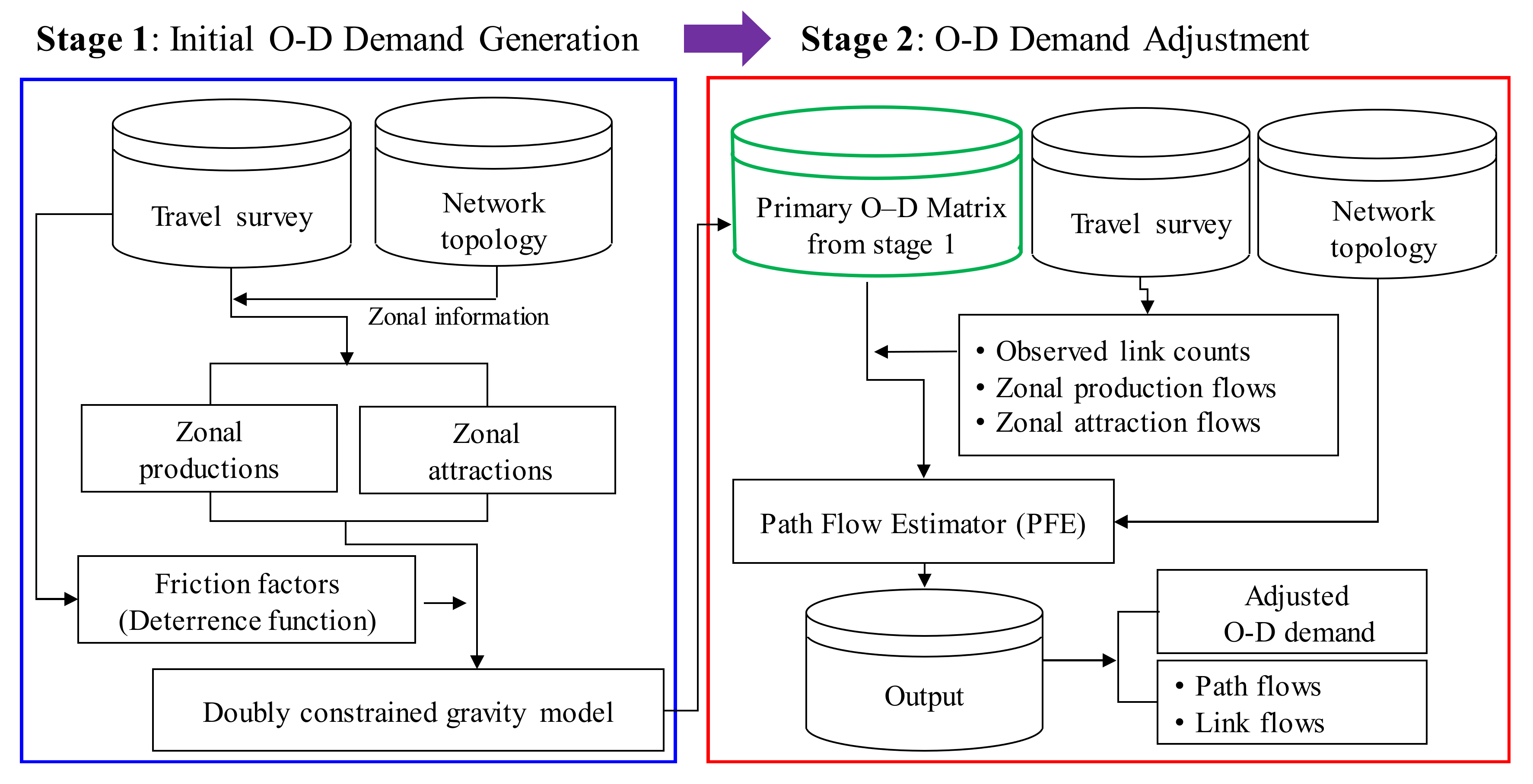
Estimating bicycle demand consists of two main stages (Figure 1). In the first stage, a doubly constrained gravity model is adopted to generate a primary bicycle O–D matrix, and then PFE is used to refine the primary bicycle O–D matrix.
2.1. Stage 1: Generation of a Primary Bicycle O–D Matrix
As shown in Figure 1 (left panel), a doubly constrained gravity model is adopted to generate the primary bicycle O–D matrix with planning data (i.e., zonal productions and zonal attractions) and calibrated impedance function or friction factors as inputs. The simplified procedure involves the following steps:
- Step 1. Estimation of zonal productions and zonal attractions using existing planning data;
- Step 2. Estimation of a primary O–D matrix in the gravity model.
Step 1 utilizes a trip generation model focusing on travel choice to perform the first step in the conventional transportation planning model (also known as the four-step model). From the trip generation model, the number of trips in a traffic analysis zone (TAZ) are predicted. If there is no direct demand available between zones, typical methods can be used to model trip generation. These methods include: (1) regression models, and (2) category (or cross-classification) models. Once the trip productions and attractions are estimated, Step 2 distributes the trips through a trip distribution model. For the trip distribution step, the gravity model (i.e., doubly constrained gravity model) is widely used as follows:
where
- Tij = Number of trips produced between zone i and zone j
- Pi = Number of trips produced in zone i
- Aj = Number of trips attracted to zone j
- Fij = An empirically derived “friction factor,” which expresses the average area-wide effect of spatial separation on the trip interchanges between the two zones, i and j
- Ki, Kj = Empirically derived origin and destination adjustment factor in zone i and zone j
Generally, the trip distribution model is a required calibration process with Fij, Ki, and Kj, but it is usually time-consuming [35]. In addition, the calibration process requires many factors, which is not established from travel surveys. In Stage 2, we introduce the alternative method, which is the refinement of the primary matrix.
2.2. Stage 2: Bicycle O–D Matrix Refinemnet
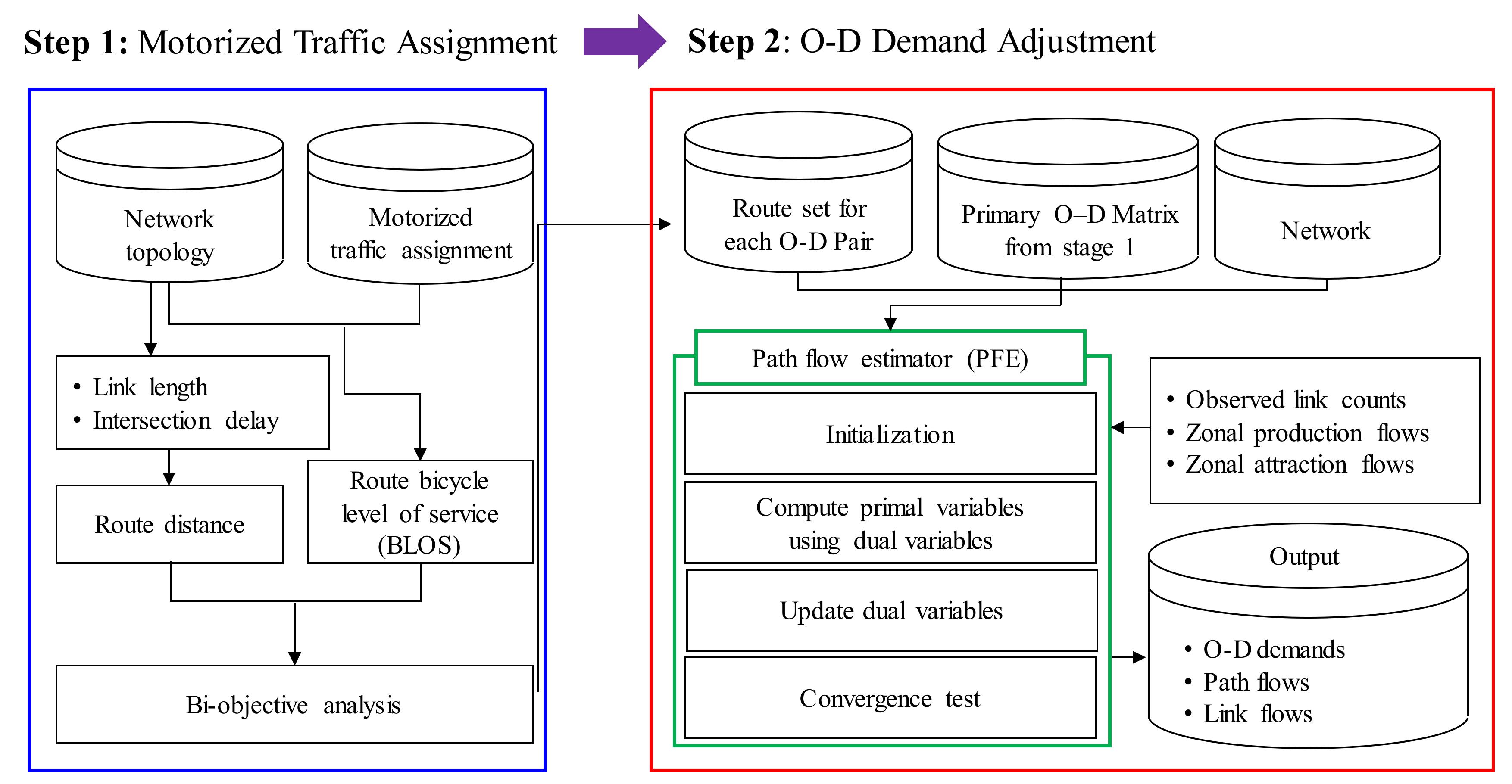
To refine the primary bicycle O–D matrix with observed bicycle counts, we developed a sequential model consisting of route generation and O–D demand adjustment. The route generation process considers two main factors, which are distance-related factors and safety-related factors). With these two factors, efficient routes for an O–D pair are generated. Once the route generation process is completed, PFE is adopted to adjust the primary bicycle O–D demand generated in Stage 1, and the adjusted bicycle O–D demand matrix in the second stage can assign more consistent link flows with observed link count data.
Stage 2 consists of two steps. In Step 1, the bicycle routes are generated based on two key factors, which are distance-related factors (i.e., route distance) and safety-related factors (i.e., bicycle level of service (BLOS)), and then O–D demand is adjusted with the primary O–D matrix generated in Stage 1, observed link counts, and zonal productions and attractions data. Figure 2 shows the overall flowchart of the bicycle O–D matrix adjustment procedure in Stage 2.
2.3. Route Generation in Stage 2
Because of the many factors [36,37,38,39,40,41,42] affecting a cyclist’s route choice, using a single objective may have limitations to construct cyclist route choice behavior [18]. Ehrgott et al. [43] introduced the bi-objective bicycle route generation model based on the route distance and route suitableness criteria. In this paper, distance-related factors (i.e., route distance) and safety-related factors (i.e., BLOS) are adopted to construct cyclist route choice behavior.
2.3.1. Route Distance
Route distance consists of the sum of link distances and the delays at intersections the route passes through. The delays at intersections have been shown to be an unfavorable factor in cycling route decision-making. Because the unit of link length (e.g., kilometer) and intersection delay (e.g., second) are different, it needs to match the same unit between two measurements. In the paper, the delay (i.e., minute) is converted to distance unit (i.e., kilometer) with a conversion factor. The details, which are equation and description of route distance, can be found in [44].
2.3.2. Bicycle Level of Service (BLOS)
There are many measurements to assess the safety or the suitability effect of bicycle facilities. Lowry et al. [45] provided thirteen methods used in the literature. Among the numerous measurements, the BLOS measure developed by the Highway Capacity Manual (HCM) [46] is used as a surrogate measure to account for safety. The BLOS measurement is introduced in the HCM as a guide for bicycle facility design. The details in terms of the BLOS development can be shown in the HCM [46].
2.3.3. Bi-Objective Shortest Path
The bi-objective shortest path problem may not have a single solution which dominates all other solutions. Therefore, the solution requires a set of nondominated (or Pareto) solutions. Several solution algorithms [47,48,49,50] have been developed, but it is not easy to solve with nonadditive route cost, which is route BLOS in the bi-objective shortest path problem. Readers may refer to Raith and Ehrgott [51] for a comparison of different solution strategies for solving the bi-objective shortest path problem. In the paper, we modified the ranking method proposed by Climaco [47]. First, routes are generated based on the route distance attributes (i.e., link distance and intersection turning movement penalty) without exceeding the maximum upper bound (i.e., 10 kilometers in this study) by using the k-shortest path algorithm, then BLOS scores are calculated for each corresponding route in the set to determine the nondominated routes.
2.4. Bicycle O–D Demand Adjustment Using Path Flow Estimator (PFE)
The PFE originally developed by Bell and Shield [52] is a one-stage network observer using traffic counts. The main component of the PFE is a logit-based path choice model in which the perception errors of path travel times are assumed to be independent Gumbel variates. Note that one of the major issues in bicycle route choice decisions is the route overlapping problem (see [53]). Hence, the aim of this section is to extend the logit-based PFE model to implement the route overlapping issue by using the path-size logit (PSL) model, and to refine the primary bicycle O–D matrix. The PSL-based PFE formulation is shown with several side constraints as follows.
where
where
- = Bicycle flow on route k connecting O–D pair rs
- = Utility route k connecting O–D pair rs
- = Path-size factor on route k connecting O–D pair rs
- = Observed bicycle count on link a
- = Estimated bicycle flow on link a
- = Percentage error of the bicycle count on link a
- and = Bicycle trip productions and bicycle trip attractions obtained from census data in origin r and destination s, respectively
- and = Refined bicycle trip productions and refined bicycle trip attraction in origin r and destination s, respectively
- and = Error bounds allowed for trip productions and trip attractions in origin r and destination s, respectively
- = Target O–D flows connecting O–D pair rs, which are initially estimated bicycle O–D demand in Stage 1.
- = Refined bicycle O–D flows connecting O–D pair rs
- = Percentage error bound for the target O–D demands connecting O–D pair r
- = Path-link indicator, 1 if link a is on path k connecting O–D pair rs and 0 otherwise.
- = Set of network links
- and = Sets of origin and destination zones
- = Set of target O–D pairs
The objective function in Equation (2) consists of three terms. The first term, which is the entropy term, distributes the O–D demand onto multiple routes with the provided dispersion parameter. The second term, which is the system optimal term, minimizes users’ utilities, and the third term, which is the Path-Size (PS) term, considers the route overlapping.
The PS factor is determined by the length of links within a path, as follows:
where
- = PS factor of path k connecting O–D pair rs
- la = Length of link a
- = Length of path k connecting O–D pair rs
Path-size factor is determined by the length of links the route passes through [17]. Hence, a path heavily overlapped with other paths has a smaller PS value, while paths that are more distinct have a larger PS value.
Compared to the traditional traffic assignment model (i.e., logit-based stochastic user equilibrium [54]), the adopted PSL-based PFE model finds path flows while reproducing observed bicycle counts in Equation (3), zonal productions and attractions in Equations (4) and (5), and target demands in Equation (6) within predefined error bounds, simultaneously. These error bounds indicate confidence levels of the observed data. If the provided data are more reliable, a smaller error bound is used to constrain the estimated flows within a narrower range, while a less reliable dataset will use a larger error bound to allow for a larger range of the estimated flows. Equation (7) constrains the path flows to be of non-negativity. Equations (8)–(11) are definitional constraints that sum up the estimated path flows to obtain the O–D demand, link flows, zonal production flows, zonal attraction flows, and O–D demands, respectively.
By constructing the Lagrangian function of the above formulation in Equations (2)–(11), path flows can be derived analytically as a function of route costs and dual, as follows.
where ,, and ,, are the dual variables representing the lower and upper limits of constraints (Equations (5)–(8)), respectively.
3. Numerical Results
To demonstrate the proposed bicycle O–D estimation model, a real network in the City of Winnipeg, Canada, was adopted in the numerical experiments. The network consists of 1067 nodes, 2555 links, and 154 zones. Among the 2555 links, 541 links are set up as bicycle links. The O–D trip table for motorized vehicles and link performance parameters were obtained from Emme/4 [55]. The bicycle network information was obtained from the City of Winnipeg [56], in Canada.
3.1. Stage 1: Generate a Primary O–D Demand
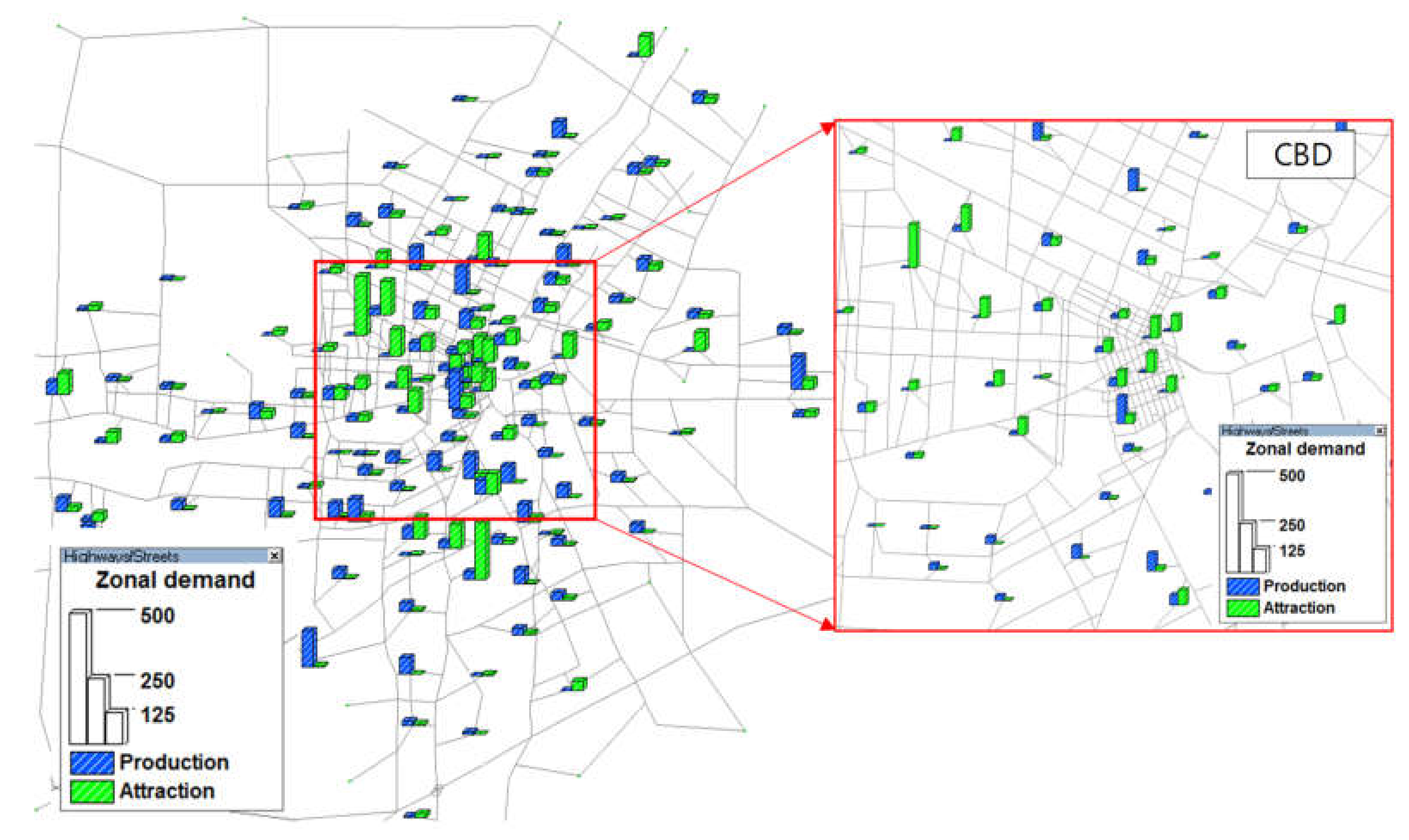
We generated a primary bicycle O–D matrix in the Winnipeg network as follows, in Stage 1. First, the zonal productions and zonal attractions were generated. The data for the total number of commuters and the percentages of commuters for each mode (e.g., car, transit, and bicycle) and in each neighborhood (i.e., zonal production flows) were obtained from the City of Winnipeg [57]. In Winnipeg, there are about 5575 commuters (or 1.8%) who use bicycles. From the census data, bicycle zonal production flows can be obtained. However, there is no available data for zonal attraction flows. As an alternative, we used the proportion of motorized vehicle demand obtained from Emme/4 [55] to estimate the bicycle zonal attraction flows as follows:
where is the total bicycle demand; is the bicycle attraction flows of zone s; is the total motorized vehicle demand; and is the motorized vehicle attraction flows of zone s.
Figure 3 illustrates the obtained bicycle production (blue color) and attraction demands (green color) for each zone from the 2006 census data. From the figure, the zonal demand pattern reveals that a majority of the bicycle attraction flows are from the central business district (CBD) area, while the bicycle production flows are generated from the non-CBD areas.
Once the bicycle productions and attractions are estimated from each zone in Figure 3, the primary bicycle O–D matrix is estimated using the doubly constrained gravity model given in Equation (1). Because of the absence of bicycle friction factors from the City of Winnipeg, bicycle trip length introduced by [58] was substituted for the friction factors. Note that origin and destination adjustment factors were not used in this study (i.e., Ki = Kj = 1 for all zones).
3.2. Stage 2: Refine the Primary Bicycle O–D Matrix with PFE
After generation of the primary bicycle O–D matrix in Stage 1, we transitioned into Stage 2 by applying the bi-objective route generation process to generate a set of bicycle routes. Once the efficient routes were generated, the PFE was performed with the observed counts data to refine the primary bicycle O–D matrix.
3.2.1. Efficient Route Generation
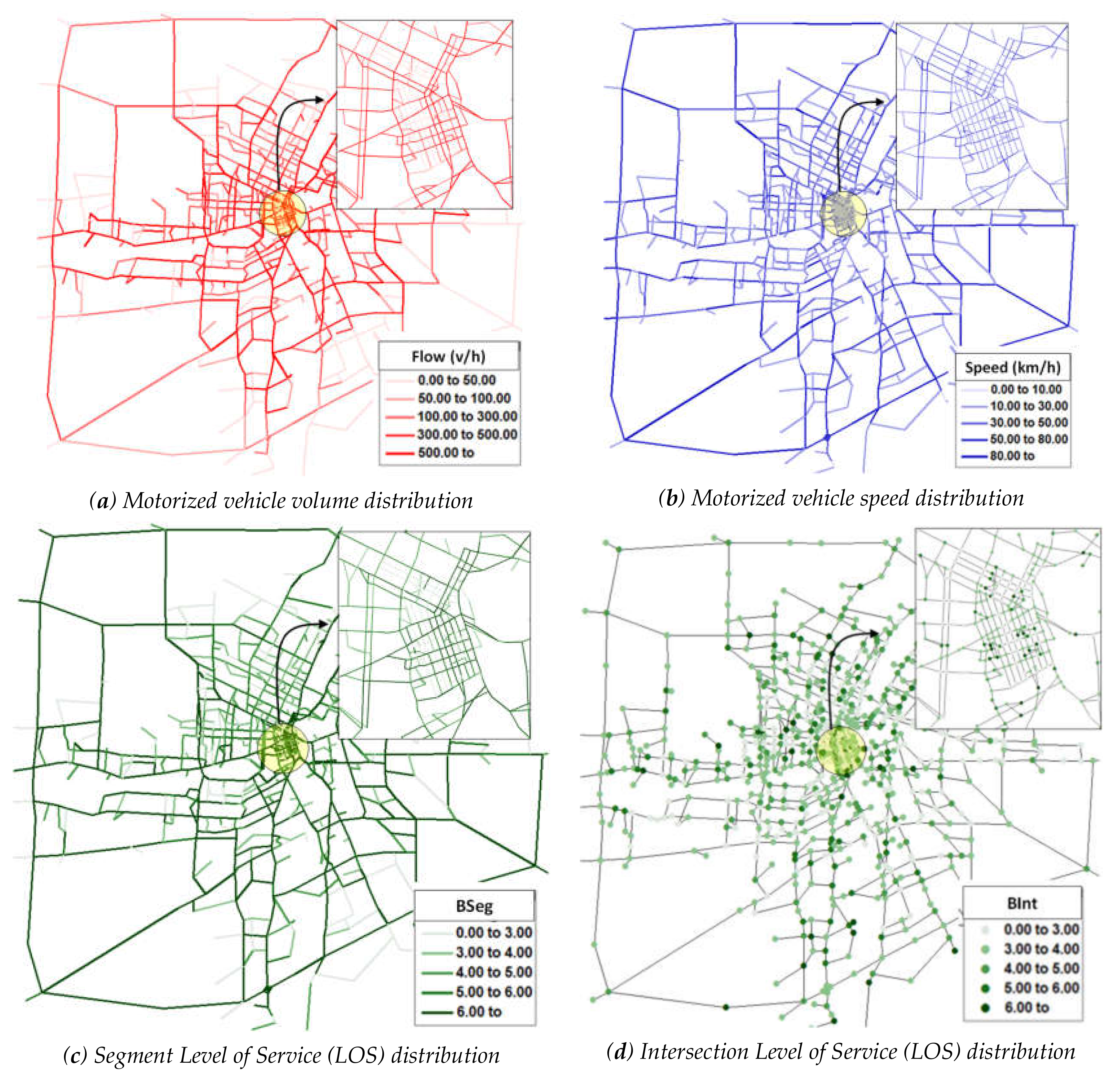
Figure 4 and Figure 5 show the transportation characteristics in the Winnipeg network. These characteristics were used to determine the route choice criteria (i.e., route distance and route BLOS). Figure 4a,b shows the vehicle volume and speed; Figure 4c,d shows the bicycle segment Level of Service (LOS) and intersection LOS from the HCM [46]. These characteristics serve for computing the two route choice criteria: route distance and route BLOS.
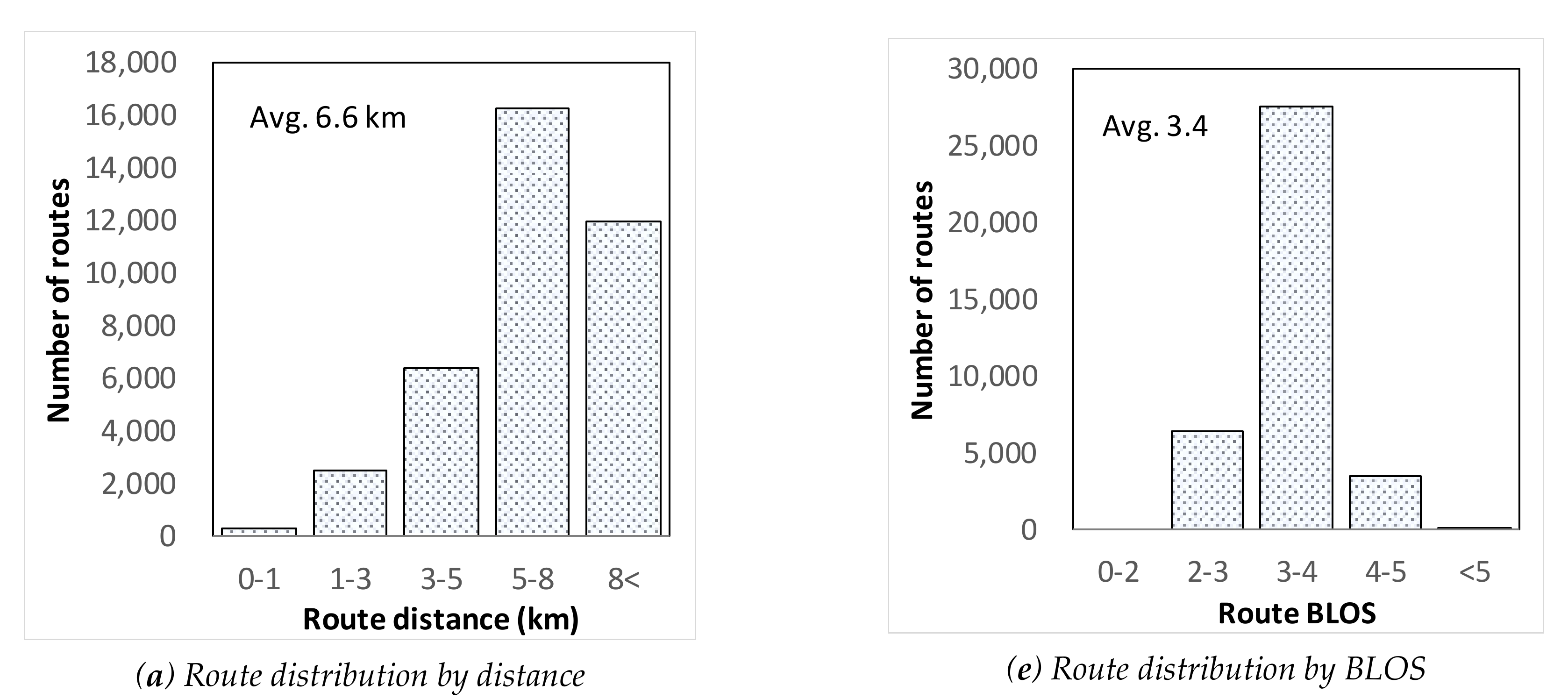
A bi-objective route generation was performed based on the characteristics of the Winnipeg network shown in Figure 5. For the upper bound of the two key criteria, we assumed 10 kilometers for route distance and 7 for route BLOS. In other words, routes with higher than 10 kilometers for route distance and routes with higher than 7 for route BLOS were excluded from the generation of the efficient route set. For the network, the bi-objective shortest path problem was performed for each O–D pair (there are 7368 O–D pairs in the Winnipeg network, hence, it was performed a total of 7368 times). From 7368 O–D pairs, the total number of generated efficient routes are 37,263 routes, and this result implies that each O–D pair has an average of about 5 efficient routes. Figure 5 shows the route distribution of the 37,263 routes. Most routes are between 5.0 and 8.0 kilometers, the average route distance is 6.6 km in terms of length, the routes have values ranging from 3.0 to 4.0, and average BLOS is 3.4.
3.2.2. Link Counts Data
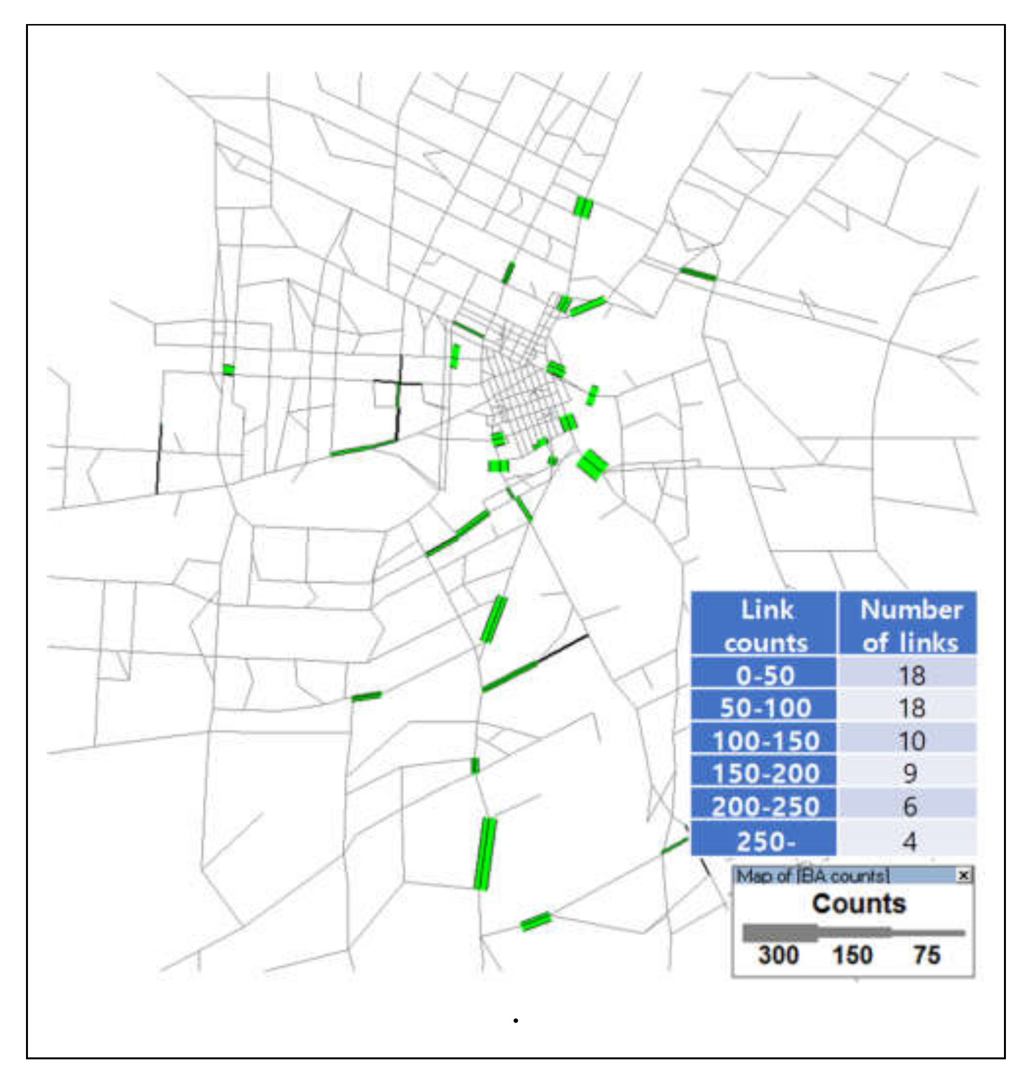
Generally, most traffic count collections are for motorized vehicles. Hence, bicycle count data may not be collected regularly, but we expect the collecting bicycle counts to increase in the future. Hull [59] analyzed cycling commuter patterns from 2007 to 2013 with 65 link count locations. From their work, we obtained observed counts data (highest counts recorded in 2007–2013) corresponding to the 65 link count locations. Figure 6 shows the obtained bicycle counts and corresponding locations.
3.2.3. Utility Parameters and Error Bounds of Observed Data
With generated efficient routes, the bicycle PFE was applied to refine the primary bicycle O–D matrix to meet the error bound of bicycle counts (Table 1), target or primary O–D demand, and zonal productions and attractions. A composite utility function was used, as suggested by Kang and Fricker [60], , where and β are parameters. We also used the parameter values (i.e., = 0.862 and β = 0.117), suggested by Kang and Fricker [60]. Because of flexibility of error bound in PFE, we can provide different error bounds for different data. A more reliable dataset will constrain the estimation to be within a smaller error bound, while a less reliable dataset will have a larger error bound (i.e., estimated values are allowed to have a large deviation). For bicycle counts, zonal productions, and attractions, error bound of 30% was used. For target O–D demands (i.e., primary bicycle O–D matrix), a flow-dependent error bound was adopted from 30% (flows are higher than 30) to 60% (flows are lower than 30).
3.3. Comparisons of Analysis Results
After performing the two-stage bicycle O–D estimation, we analyzed the differences between: (1) the observed flows and the estimated flows; (2) the primary matrix and the refined matrix; and (3) the link flows by Path Size Logit-based Assignment (PSLA) and the link flows by PFE.
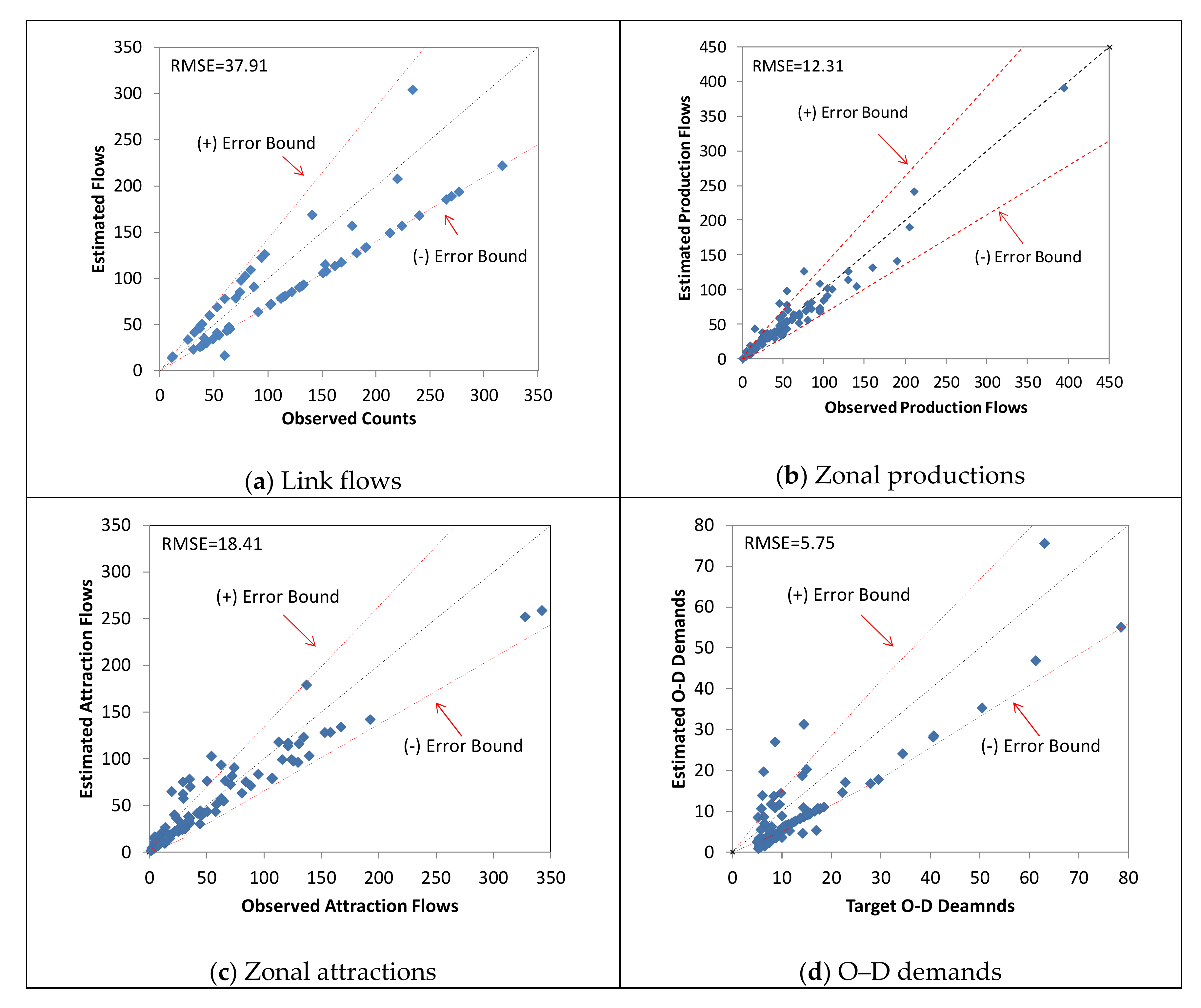
Our first comparison delves into the differences between the observed flows to the estimated flows. Figure 7 shows the scatter plots in link flow, zonal productions, zonal attractions, and O–D demands. The root-mean-square error (RMSE) value is provided for accuracy.
Figure 7 supports the notion that the two-stage process generates few differences between observed and estimated flows. Most of the estimated well match the observed data within given error bounds. The RMSE are 37.91 for estimated link flows, 12.31 for estimated zonal productions, 18.41 for estimated zonal attractions, and 5.75 for O–D demand. However, there were some estimated flows that did not match. Because the data used for link counts represent the counts during 2007–2013, and because the zonal production flows were obtained in 2006, there is counts inconsistency in the dataset. For this reason, some of estimated zonal attractions and refined O–D demand are out of error bound. In addition, most estimated link flows are concentrated near the lower error bound, while estimated planning flows (i.e., zonal productions and attractions) are near the upper error bound, and some flows are beyond the upper error bound. From the results, we can infer that the planning input data, which were obtained in 2006, are relatively smaller than that of the observed counts input data, which were obtained between 2007 and 2013.
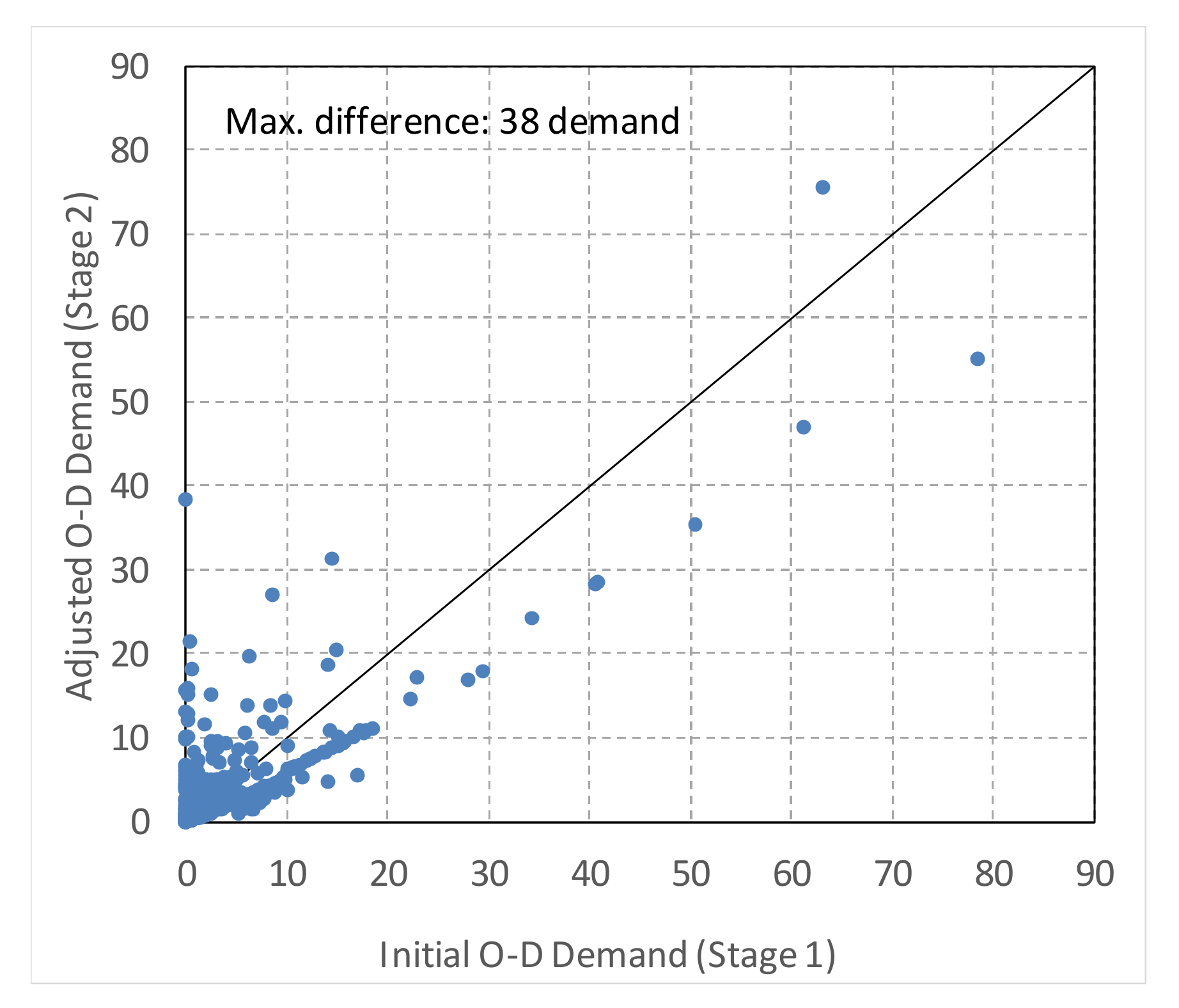
In our second comparison, we evaluated the differences between the primary O–D demand and the refined O–D demand. Figure 8 shows the scatter plots of the primary O–D demand and the refined O–D demand. About 88% of the O–D pairs are adjusted within ±0.25 trips, and more than 95% of the O–D pairs are within ±1.0 trips. However, the demand for about 2% of O–D pairs (174 O–D pairs) is significantly adjusted.
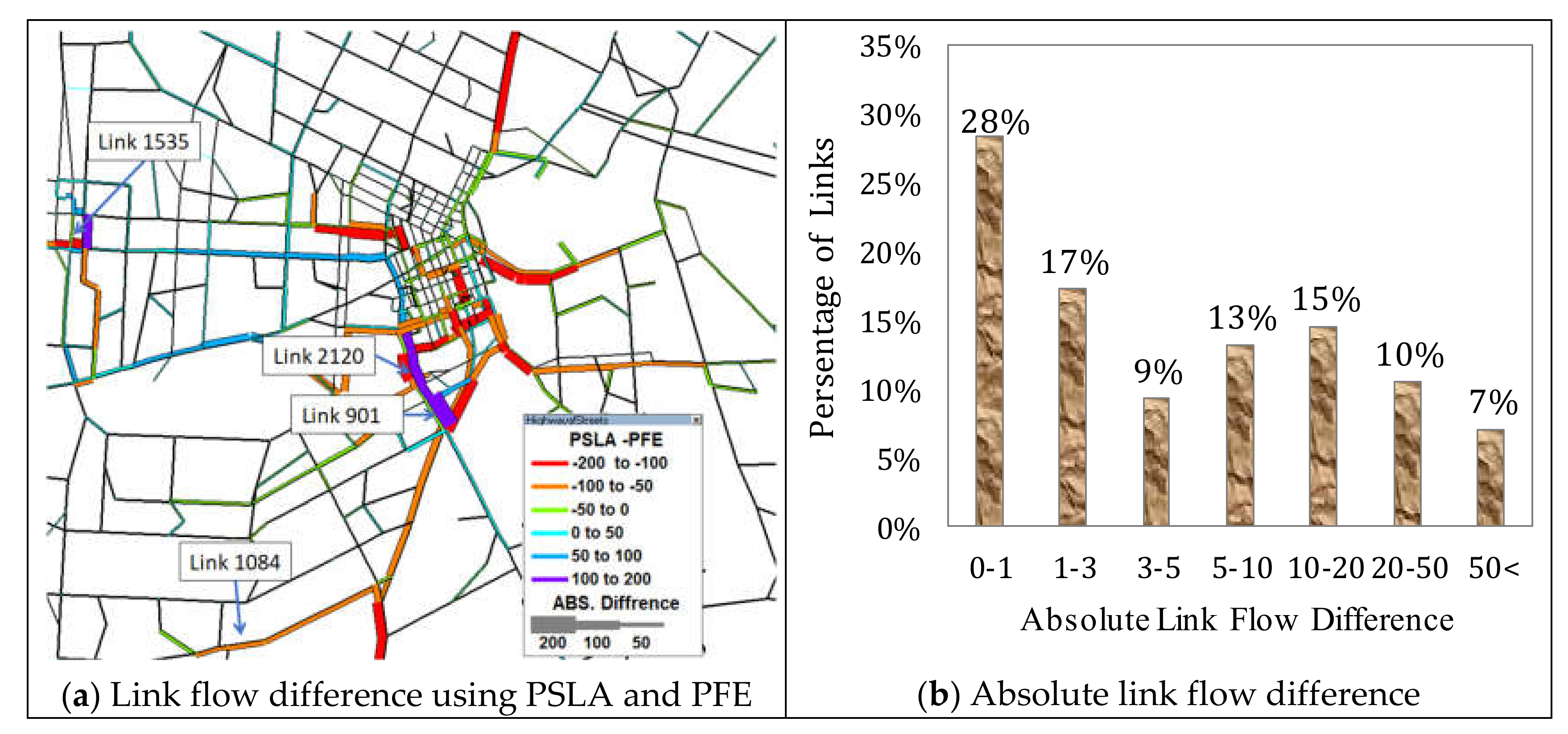
For the third comparison, the assigned link flows by PSL assignment and the estimated link flows by PFE were compared. Figure 9a shows the link flow comparison between these two methods. On the map, the red and orange colors indicate that the assigned link flows by PFE model have greater flows than the assigned link flows by PSL model. The purple and blue colors indicate the reverse. As can be seen, there are more flow adjustments in the CBD area. Because most traffic count locations are located near CBD areas, and because areas near CBD areas have relatively higher demand than other areas, these areas are more affected in O–D demand adjustment. Figure 9b provides a more detailed analysis through a bar graph, displaying the link flow difference distribution. Only 28% of links have 0–1 flow difference, while about 32% of links have significant difference.
4. Conclusions
The paper presents a methodology for bicycle demand estimation from observed data. The estimation process involves two key stages: a primary bicycle O–D estimation and a refinement of the estimated primary bicycle O–D demand. The first stage generates the primary O–D demand in a gravity model with available planning data as input. The second stage then generates efficient routes (considering route distance and route BLOS) and uses PFE to refine the primary O–D trips generated in the first stage with observed counts data. This two-stage process enhances the accuracy of the results by making the route flows estimated by the O–D demand matrix more consistent with the observed flows.
A case study was conducted on a real network in the City of Winnipeg, Canada, to show proof of concept. In the City of Winnipeg network, incorporating bicycle counts in bicycle O–D matrix estimation results in significantly different flow patterns. Because of the absence of a calibration process in the trip distribution step and traffic assignment step, the reason for the significantly different flow patterns between estimated and observed link flows is probably supported. The findings in this study have important implications in bicycle planning. The proposed two-stage process is demonstrated to be a useful tool in modeling cyclist planning such as bicycle facility construction, navigating bicycle routes, and can be used to guide the design of networks and to guide bicycle travel more efficiently. For future research on bicycle O–D estimation, we recommend the following five considerations. Firstly, we recommend conducting parameter calibration, because we believe that the absence of calibration in this research had significant effects on the results. Secondly, it would be more realistic to incorporate a variety of network topologies and bicycle facilities into the analysis. Thirdly, we recommend integrating the congestion effect of motorized vehicles as well as a more comprehensive look at travel patterns. On a similar note of increased inclusivity, we also recommend incorporating travelers’ driving skills. Lastly, we recommend implementing more data collection to avoid data inconsistency problems.
Funding
This research was funded by the Basic Science Research Program, grant number NRF-2016R1C1B2016254; And Development of Data-driven Solution for Social Issue in Korea Institute of Science and Technology Information, grant number K-20-L01-C06-S01
Conflicts of Interest
The authors declare no conflicts of interest.
References
- Braun, L.M.; Rodriguez, D.A.; Cole-Hunter, T.; Ambros, A.; Donaire-Gonzalez, D.; Jerrett, M.; de Nazelle, A. Short-term planning and policy interventions to promote cycling in urban centers: Findings from a commute mode choice analysis in Barcelona, Spain. Transp. Res. Part A 2016, 89, 164–183. [Google Scholar] [CrossRef] [Green Version]
- Kager, R.; Bertolini, L.; Te Brömmelstroet, M. Characterisation of and reflections on the synergy of bicycles and public transport. Transp. Res. Part A 2016, 85, 208–219. [Google Scholar] [CrossRef] [Green Version]
- Martens, K. Promoting bike-and-ride: The Dutch experience. Transp. Res. Part A 2007, 41, 326–338. [Google Scholar] [CrossRef]
- Pucher, J.; Buehler, R.; Seinen, M. Bicycling renaissance in North America? An update and re-appraisal of cycling trends and policies. Transp. Res. Part A 2011, 45, 451–475. [Google Scholar] [CrossRef]
- The League of American Bicyclist. Becoming a Bicycle Friendly Community. Available online: http://www.bikeleague.org/commutingdata (accessed on 12 December 2016).
- Turner, S.; Hottenstenin, A.; Shunk, G. Bicycle and Pedestrian Travel Demand Forecasting: Literature Review; Texas Transportation Institute: College Station, TX, USA, 1997; Available online: http://d2dtl5nnlpfr0r.cloudfront.net/tti.tamu.edu/documents/1723-1.pdf (accessed on 10 January 2014).
- Cambridge Systematics, Inc. Guidebook on Methods to Estimate Non-Motorized Travel: Supporting Documentation; Federal Highway Administration: McLean, VA, USA, 1999. Available online: http://safety.fhwa.dot.gov/ped_bike/docs/guidebook2.pdf (accessed on 10 January 2014).
- Wigan, M.; Richardson, A.; Brunton, P. Simplified estimation of demand for non-motorized trails using GIS. Transp. Res. Rec. 1998, 1636, 47–55. [Google Scholar] [CrossRef]
- Epperson, B. Demographic and economic characteristics of bicyclists involved in bicycle-motor vehicle accidents. Transp. Res. Rec. 1995, 1502, 58–64. [Google Scholar]
- Nelson, A.C.; Allen, D. If you build them, commuters will use them: Cross-sectional analysis of commuters and bicycle facilities. Transp. Res. Rec. 1997, 1578, 79–83. [Google Scholar] [CrossRef]
- Goldsmith, S. Estimating the Effect of Bicycle Facilities on VMT and Emissions; Seattle Engineering Department: Seattle, WA, USA, 1997. [Google Scholar]
- Noland, R.B. Perceived risk and modal choice: Risk compensation in transportation systems. Accid. Anal. Prev. 1995, 27, 503–521. [Google Scholar] [CrossRef]
- Kitamura, R.; Mokhtarian, P.; Laidet, L. A micro-analysis of land use and travel in five neighborhoods in the San Francisco Bay Area. Transportation 1997, 24, 125–158. [Google Scholar] [CrossRef]
- Clark, D.E. Estimating future bicycle and pedestrian trips from a travel demand forecasting model. In Proceedings of the Institute of Transportation Engineers 67th Annual Meeting, Boston, MA, USA, 3–7 August 1997. [Google Scholar]
- Ortuzar, J.; Iacobelli, A.; Valeze, C. Estimating demand for a cycle-way network. Transp. Res. Part A 2000, 34, 353–357. [Google Scholar] [CrossRef]
- Hood, J.; Sall, E.; Charlton, B. A GPS-based bicycle route choice model for San Francisco, California. Transp. Lett. Int. J. Transp. Res. 2011, 3, 63–75. [Google Scholar] [CrossRef]
- Ben-Akiva, M.; Bierlaire, M. Discrete choice methods and their applications to short term travel decisions. In Handbook of Transportation Science; Springer: Boston, MA, USA, 1999. [Google Scholar]
- Menghini, G.; Carrasco, N.; Schussler, N.; Axhausen, K.W. Route choice of cyclists in Zurich. Transp. Res. Part A 2010, 44, 754–765. [Google Scholar] [CrossRef]
- Fagnant, D.; Kockelman, K. A direct-demand model for bicycle counts: The impacts of level of service and other factors. Environ. Plan. B Plan. Des. 2016, 43, 93–107. [Google Scholar] [CrossRef] [Green Version]
- Griswold, J.; Medury, A.; Schneider, R. Pilot models for estimating bicycle intersection volumes. Transp. Res. Rec. 2011, 2247, 1–7. [Google Scholar] [CrossRef] [Green Version]
- Van Zuylen, H.J. The estimation of turning flows on a junction. Traffic Eng. Control 1979, 20, 539–541. [Google Scholar]
- Van Zuylen, H.J.; Willumsen, L.G. The most likely trip estimated from traffic counts. Transp. Res. Part B 1980, 14, 281–293. [Google Scholar] [CrossRef]
- Brenninger-Gothe, M.; Jornsten, K.O.; Lundgren, J.T. Estimation of origin-destination matrices from traffic counts using multi-objective programming formulations. Transp. Res. Part B 1989, 23, 257–269. [Google Scholar] [CrossRef]
- Lam, W.H.K.; Lo, H.P. Estimation of origin-destination matrix from traffic counts: A comparison of entropy maximizing and information minimizing models. Transp. Plan. Technol. 1991, 16, 166–171. [Google Scholar] [CrossRef]
- Spiess, H. A maximum likelihood model for estimating origin-destination matrices. Transp. Res. Part B 1987, 21, 395–412. [Google Scholar] [CrossRef]
- Cascetta, E.; Nguyen, S. A unified framework for estimating or updating origin/destination matrices from traffic counts. Transp. Res. Part B 1988, 22, 437–455. [Google Scholar] [CrossRef]
- Lo, H.P.; Zhang, N.; Lam, W.H.K. Estimation of an origin-destination matrix with random link choice proportions: A statistical approach. Transp. Res. Part B 1996, 30, 309–324. [Google Scholar] [CrossRef]
- Hazelton, M.L. Estimation of origin-destination matrices from link flows on uncongested networks. Transp. Res. Part B 2000, 34, 549–566. [Google Scholar] [CrossRef]
- Robillard, P. Estimation of the O-D matrix from observed link volumes. Transp. Res. 1975, 9, 123–128. [Google Scholar] [CrossRef]
- Cascetta, E. Estimation of origin-destination matrices from traffic counts and survey data: A generalized least squares estimator. Transp. Res. Part B 1984, 18, 289–299. [Google Scholar] [CrossRef]
- Hendrickson, C.; McNeil, S. Estimation of origin-destination matrices with constrained regression. Transp. Res. Rec. 1985, 976, 25–32. [Google Scholar]
- Bell, M.G.H. The estimation of origin-destination matrices by constrained generalized least squares. Transp. Res. Part B 1991, 25, 13–22. [Google Scholar] [CrossRef]
- Maher, M. Inferences on trip matrices from observations on link volumes: A Bayesian statistical approach. Transp. Res. Part B 1983, 17, 435–447. [Google Scholar] [CrossRef]
- Barbour, R.; Fricker, J.D. Estimation of an origin-destination table using a method on shortest augmenting paths. Transp. Res. Part B 1994, 28, 77–89. [Google Scholar] [CrossRef]
- Ortuzar, J.; Willumsen, L.G. Modelling Transport, 4th ed.; John Wiley & Sons: Hoboken, NJ, USA, 2011. [Google Scholar]
- Stinson, M.A.; Bhat, C.R. An analysis of commuter bicyclist route choice using a stated preference survey. Transp. Res. Rec. 1828, 1828, 107–115. [Google Scholar] [CrossRef]
- Broach, J.; Dill, J.; Gliebe, J. Where do cyclists ride? A route choice model developed with revealed preference GPS data. Transp. Res. Part A 2012, 46, 1730–1740. [Google Scholar] [CrossRef]
- Hunt, J.D.; Abraham, J.E. Influences on bicycle use. Transportation 2007, 34, 453–470. [Google Scholar] [CrossRef]
- Akar, G.; Clifton, K.J. Influence of individual perceptions and bicycle infrastructure on decision to bike. Transp. Res. Rec. 2009, 2140, 165–171. [Google Scholar] [CrossRef]
- Hopkinson, P.; Wardman, M. Evaluating the demand for cycle facilities. Transp. Policy 1996, 3, 241–249. [Google Scholar] [CrossRef]
- Dill, J.; Carr, T. Bicycle commuting and facilities in major US cities: If you build them, commuters will use them. Transp. Res. Rec. 2003, 1828, 116–123. [Google Scholar] [CrossRef]
- Winters, M.; Davidson, G.; Kao, D.; Teschke, K. Motivators and deterrents of bicycling: Comparing influences on decisions to ride. Transportation 2011, 38, 153–168. [Google Scholar] [CrossRef]
- Ehrgott, M.; Wang, J.; Raith, A.; van Houtte, A. A bi-objective cyclist route choice model. Transp. Res. Part A 2012, 46, 652–663. [Google Scholar] [CrossRef]
- Ryu, S. Modeling Transportation Planning Applications via Path Flow Estimator; Utah State University: Logan, UT, USA, 2015. [Google Scholar]
- Lowry, M.; Callister, D.; Gresham, M.; Moore, B. Assessment of community-wide bikeability with bicycle level of service. Transp. Res. Rec. 2012, 2314, 41–48. [Google Scholar] [CrossRef]
- Highway Capacity Manual; Transportation Research Board: Washington, DC, USA, 2011.
- Climaco, J.C.N.; Martins, E.Q.V. A bicriterion shortest path problem. Eur. J. Oper. Res. 1982, 11, 399–404. [Google Scholar] [CrossRef]
- Skriver, A.J.V.; Andersen, K.A. A label correcting approach for solving bicriterion shortest-path problems. Comput. Oper. Res. 2000, 27, 507–524. [Google Scholar] [CrossRef]
- Tung, C.T.; Chew, K.L. A multicriteria Pareto-optimal path algorithm. Eur. J. Oper. Res. 1992, 62, 203–209. [Google Scholar] [CrossRef]
- Ulungu, E.L.; Teghem, J. The two phases method: An efficient procedure to solve bi-objective combinatorial optimization problems. Found. Comput. Decis. Sci. 1995, 20, 149–165. [Google Scholar]
- Raith, A.; Ehrgott, M. A comparison of solution strategies for bi-objective shortest path problems. Comput. Oper. Res. 2009, 36, 1299–1331. [Google Scholar] [CrossRef]
- Bell, M.G.H.; Shield, C.M.; Busch, F.; Kruse, G. A stochastic user equilibrium path flow estimator. Transp. Res. Part C 1997, 59, 197–210. [Google Scholar] [CrossRef]
- Prashker, J.N.; Bekhor, S. Route choice models used in the stochastic user equilibrium problem: A review. Transp. Rev. 2004, 24, 437–463. [Google Scholar] [CrossRef]
- Fisk, C. Some developments in equilibrium traffic assignment. Transp. Res. Part B 1980, 14, 243–255. [Google Scholar] [CrossRef]
- Emme Software Manual; INRO Consultants: Montreal, Canada, 2014.
- City of Winnipeg. Winnipeg Cycling Map. Available online: http://www.winnipeg.ca/publicworks/MajorProjects/ActiveTransportation/maps-and-routes.stm (accessed on 12 January 2014).
- City of Winnipeg. 2006 Mobility by Neighborhood.xls in 2006 Census. Available online: http://winnipeg.ca/census/2006/Selected%20Topics/default.asp (accessed on 13 January 2014).
- Aultman-Hall, L.; Hall, F.; Baetz, B. Analysis of bicycle commuter routes using geographic information systems implications for bicycle planning. Transp. Res. Rec. 1997, 1578, 102–110. [Google Scholar] [CrossRef]
- Hull, J. Commuter Cycling in Winnipeg 2007–2013. 2013. Available online: http://bikewinnipeg.ca/wordpress/wp-content/uploads/2013/01/Commuter_Cycling_in_Winnipeg_2007-2013.pdf (accessed on 30 August 2013).
- Kang, L.; Fricker, J. A bicycle route choice model that incorporate distance and perceived risk. In Proceedings of the 92nd Annual Meeting of the Transportation Research Board, Washington, DC, USA, 13–17 January 2013. [Google Scholar]
Figure 1.
The flowchart for the bicycle origin–destination (O–D) estimation.

Figure 2.
Bicycle O–D matrix adjustment procedure in Stage 2. BLOS: bicycle level of service.

Figure 3.
Zonal bicycle productions and attractions. CBD: central business district.

Figure 4.
Characteristics of the Winnipeg network.

Figure 5.
Route distribution by route distance and route BLOS in generated route set.

Figure 6.
Observed link count locations and counts distribution

Figure 7.
Comparison between observed and estimated flows.

Figure 8.
Comparison between primary demand and adjusted demand.

Figure 9.
Link flow difference pattern and absolute link flow difference using Path Size Logit-based Assignment (PSLA) and PFE.
Figure 9.
Link flow difference pattern and absolute link flow difference using Path Size Logit-based Assignment (PSLA) and PFE.


Table 1.
Used error bound in the PFE estimation.
| Input Data | Error Bound |
|---|---|
| Bicycle counts | +/-30%: all observed links |
| Zonal production flows | +/-30%: all observed zones |
| Zonal attraction flows | +/-30%: all observed zones |
| Target O–D demand | Error-free: if demands are between 0 and 5 +/-60%: if demands are between 5 and 30 +/-30%: if demands are higher than 30 |
© 2020 by the author. Licensee MDPI, Basel, Switzerland. This article is an open access article distributed under the terms and conditions of the Creative Commons Attribution (CC BY) license (http://creativecommons.org/licenses/by/4.0/).
Share and Cite
MDPI and ACS Style
Ryu, S. A Bicycle Origin–Destination Matrix Estimation Based on a Two-Stage Procedure. Sustainability 2020, 12, 2951. https://0-doi-org.brum.beds.ac.uk/10.3390/su12072951
AMA Style
Ryu S. A Bicycle Origin–Destination Matrix Estimation Based on a Two-Stage Procedure. Sustainability. 2020; 12(7):2951. https://0-doi-org.brum.beds.ac.uk/10.3390/su12072951
Chicago/Turabian StyleRyu, Seungkyu. 2020. "A Bicycle Origin–Destination Matrix Estimation Based on a Two-Stage Procedure" Sustainability 12, no. 7: 2951. https://0-doi-org.brum.beds.ac.uk/10.3390/su12072951
Note that from the first issue of 2016, this journal uses article numbers instead of page numbers. See further details here.