Emission Embodied in International Trade and Its Responsibility from the Perspective of Global Value Chain: Progress, Trends, and Challenges

Abstract

In the context of economic globalization and production fragmentation, the boom in intermediate and processing trade has made EEIT (emission embodied in international trade) accounting and the recognition of its responsibility more and more complicated, and the drawbacks of traditional gross value statistics more and more conspicuous. The rapid development of global value chain theory in recent years has given rise to a decomposition framework of the trade flow in a country’s export, based on the global value chain, which offers new methods to study EEIT and allocate its responsibility. The combination of global value chain accounting and EEIT research can offer new ways to research EEIT transfer and allocate its responsibility. Utilization of this technique can help understand each country’s “common but differentiated responsibility” in emission reduction. Finally, aiming at the knowledge gaps in current analysis, this paper attempts to discuss the trends, and possible challenges, in research on EEIT, and its responsibility based on the global value chain theory.

1. Introduction

Owing to the rapid development of the global economy and industrialization, the large quantify of emissions resulting from human activities have become a leading cause of global climate change. In August 2018, the IPCC released the special report “Global Warming of 1.5 °C” [1]. This jump in global warming encouraged the acceleration of global action to combat climate change, and supported the move towards more stringent global emission reduction steps. Combating climate change is a significant issue in the current international political economy, with international trade in goods, services, capital, and its attendant emission responsibilities, acting as the bones of contentions among countries. The goods, services, and capital of each country are transferred among countries through international trade. Moreover, emission embodied in these trade flows, i.e., EEIT (emissions embodied in international trade) is also transferred among countries—changing the global economy and environment. Any effort to reduce emissions implies designing policies that allocate responsibility to actors involved in causing these emissions [2], and research on EEIT is indispensable for distinguishing these responsibilities. Therefore, EEIT and emission responsibility have evolved into two important issues in the international trade and carbon emission research areas, attracting huge attention.

The measurement of EEIT mainly uses life cycle assessment (LCA) and input-output analysis (IOA). LCA is a bottom-up method based on the product life cycle, providing specific information for policy-makers. LCA requires vast detailed data and high data integrity; however, there is no unified database at present. Moreover, a systematic phase error exists in LCA as a consequence of the boundary partition insufficiency, making it difficult to calculate emissions using LCA. IOA, by contrast, can completely capture the input-output information of the entire production process and has relatively low data requirements. Therefore, IOA is the main method used in current EEIT research [3,4].

Numerous studies use IOA to calculate EEIT, and almost all of them rely on traditional trade statistics. These traditional trade statistics use the gross value of goods and services as the statistical caliber, while processing trade makes intermediate goods and services may flow across the boundaries multiple times, resulting in the “double counting” problem [5,6,7]. Current emission responsibility is allocated according to EEIT calculations based on traditional trade statistics—and is, thus, susceptible to the “double counting” problem, so it clearly cannot fairly and truly consider the real benefits and environmental costs of international trade among countries. This problem is particularly acute in the case of developing countries, a majority of which are dominated by the processing trade. To establish a fair and effective responsibility allocation mechanism, it is significant to clarify how much EEIT is caused through which route in each country, and global value chain (GVC) theory is an effective method for determining this information.

The rise and evolution of GVC has become an important feature of current international trade, as a consequence of the gradual deepening of the global division of labor. The previously mentioned deficiencies in traditional trade statistics render them unable to reflect the current situation of international trade featured by GVC. New methods are in need to measure international trade flows in the context of fragmented global production [7]. The WTO and OECD jointly presented such a new method based on the concept of “trade in value-added (TiVA)” [8]. Moreover, since then, the study on GVC accounting based on TiVA has been further developed.

The deficiency of traditional trade statistics grows in tandem with trade globalization, and the progress of GVC accounting provides new solutions for relevant research. In September 2018, China’s State Council Information Office issued “The Facts and China’s Position on China–US Trade Friction”, deeply analyzing the real China–US trade situation from the GVC perspective [9]. The GVC theory has become increasingly important in the negotiation of international trade disputes and global climate change. Predictably, the relationship between international trade, EEIT, and GVC will become increasingly close in the future. There are many studies about EEIT and emission responsibility, and some of them offer detailed reviews and analyses of relevant research [10,11,12,13,14,15,16,17,18,19,20]. However, most of the existing reviews rarely make a comprehensive analysis of both EEIT and its responsibility, instead only focusing on one of them. Emission responsibility is closely intertwined with EEIT accounting, especially in the context of economic globalization and production fragmentation. A comprehensive analysis of EEIT, emission responsibility, and GVC theory may generate new solutions for global actions to reduce emissions and combat climate change, but a detailed review of related research does not yet exist.

This paper provides a detailed review of EEIT, emission responsibility, and GVC related literature from a global perspective to clarify progress in the domain and discuss the trends and challenges of research on EEIT and its responsibility from the GVC perspective. The remainder is organized as follows: Progress in EEIT research is analyzed in Section 2; progress in emission responsibility research is shown in Section 3; progress in GVC accounting and its utilization in EEIT and emission responsibility is provided in Section 4; Section 5 provides the conclusion and further perspectives.

2. Emission Embodied in International Trade

The concept “embodiment” was firstly presented by the International Federation of Institutes for Advanced Studies (IFIAS), which used “embodied energy” to represent the energy required directly and indirectly to allow a system to produce a specific good or service. “Embodied emission” is an extension of this concept and is used to measure the emission produced by a product or service throughout its whole production process. With the rapid development of international trade and the mass adoption of global emission reduction, EEIT has become a more and more common research subject. Zhang et al. (2019) provided a bibliometrics analysis of EEIT research and pointed that relevant studies mainly focused on two aspects: The calculation of EEIT and the decomposition analysis of EEIT driving factors [21]. Relevant literature is reviewed according to this classification in the following.

2.1. The Calculation of EEIT

The calculation of EEIT is still at the estimation level, and IOA is the most common method. IOA is firstly proposed by Leontief and is used to analyze the balance of product supply and demand among various sectors by compiling the IO tables. In the late 1960s, IOA was applied to energy and environmental research and became a fundamental approach in this domain [22,23,24]. The IO model can be roughly divided into the single-region input-output (SRIO) model and the multi-region input-output (MRIO) model.

The SRIO model is used to study the emissions embodied in the foreign trade of a country (or region) and treats all other countries and regions as a single entity. According to the processing method of imports, the SRIO model can be further classified as the competitive IO model and non-competitive IO model. Based on the assumption that imports and domestic products are at the same level of production technology, the competitive IO model makes no distinction of imports in intermediates and final use products. Because of the easy and direct acquisition of competitive IO tables, the competitive IO model was commonly used in early studies. For example, Schaeffer et al. (1996), Julio et al. (2004), and Mongelli et al. (2006) used this method to calculate the EEIT of Brazil, Spain, and Italy, respectively [25,26,27]. The non-competitive IO model distinguishes import products from domestic products, and in the absence of data, an assumption about the component of imports is in need when using this model. However, import data is rarely divided along these lines, so compiling sorted data (or applying the assumed proportion of intermediate and final use imports to unsorted data) requires a large workload. For a competitive IO model to ignore the influence of imports in the production process when calculating EEIT is generally believed to be unreasonable, leading to a significant increase in the use of non-competitive IO model in calculating EEIT. Weber et al. (2008), Pan et al. (2008), Su et al. (2010), Wei et al. (2011), Dietzenbacher et al. (2012), Liu et al. (2013), and Jiang et al. (2015) used this method to calculate the EEIT of China and unanimously pointed out that China is a net exporter of EEIT [28,29,30,31,32,33,34]. Su et al. (2013) analyzed the embodied emissions of China’s exports, respectively based on competitive and non-competitive IO models—revealing that the estimated results of the competitive IO model were higher than those of non-competitive model. This difference was attributed to the transition of intermediate products between export and import [35]. The SRIO model makes another potential assumption that the energy consumption coefficient (emission coefficient) of imported products is the same as the energy consumption coefficient (emission coefficient) of domestically produced products. Simply put, it assumes that the imported products are produced using the same production technology and energy input as domestically produced products. Lin et al. (2010) used China’s emission intensity instead of the relevant import producers’ data to calculate the emissions avoided by import [36]. Although the emissions avoided by China’s import can be estimated based on this assumption, the amount tends to be overestimated, since China’s emission intensity is significantly higher than that of most producers of imports to China. As the products imported by a country come from many countries and regions in the world, different production technologies among them lead to different energy consumption and emission coefficients. For the sake of higher accuracy, scholars have improved the SRIO model in some ways, such as dividing imports into intermediate inputs and final consumption goods or calculating the emissions embodied in imported products by using the importing country’s energy consumption and emission coefficients. Yan et al. (2010) used the typical country alternative method, namely, using the emission intensity of a typical country or the average of several typical countries, to calculate the emission embodied in imports of China [37]. Jiang et al. (2015) directly used the relevant data of exporting countries to calculate the emission embodied in the import of China [34]. These improvements calculate the import embodied emissions more accurately, to some extent—however, the presupposition of import homogeneity implicit in the SRIO model leads to inevitable inaccuracies in its results, most notably when estimating EEIT transfers between countries with obviously different technology levels and energy structure.

Compared to the SRIO model, the MRIO model, which is featured in more studies, describes the industrial relations and trade links among various sectors of multiple countries from a global perspective. This model, however, is more complex than the SRIO model and requires higher data quality. The MRIO model can be divided into the Bilateral IO model and the Multinational IO model. The Bilateral IO model studies the EEIT between two specific countries, which is more targeted and has certain reference significance for international trade policy-making. Shui et al. (2006) adopted this model to study the EEIT in China–US bilateral trade from 1997 to 2003 [38]. Li et al. (2008) used this method to study the EEIT between China and the UK [39]. Yin et al. (2010) and Zhan et al. (2014) also studied the EEIT between China and the United States [40,41]. Ding et al. (2018) calculated EEIT of China with 219 trading partners to explore the impact of international trade on China’s emissions and applied the “no-trade scenario” hypothesis to explore China’s bilateral trade influence, as well as the possible contribution on the global emissions [42]. Due to the international transfer of embodied emissions brought on by the current trend of trade globalization, however, a simple Bilateral IO model cannot meet the demands of complex EEIT measurement in multinational trade, so there is a tendency toward the use of Multinational IO models in the current mainstream research.

The multinational IO model calculates EEIT based on the consideration to differentiate the technology differences between domestic products and imported products from different regions, dividing imported products into final consumption and intermediate inputs [4]. Ahmad et al. (2003) and Nakano et al. (2009) used the Multinational IO table compiled by the OECD to calculate the EEIT of 24 and 41 countries/regions, respectively [43,44]. Global Trade Analysis Project (GTAP) data was used to calculate the 2001 EEIT of 87 and 113 countries/regions, respectively, in Peters et al. (2008) and Peters et al. (2011) [20,45]. Also, Dong et al. (2010) and Liu et al. (2010) respectively analyzed the EEIT in China-Japan using the Asian IO table provided by the Institute of Developing Economies and the Japan External Trade Organization (IDE/JETRO) [46,47]. Ding et al. (2017) measured the embodied emissions caused by China’s Outward Foreign Direct Investment (OFDI) by applying a Non-competitive IO model into their study of China’s OFDI [48]. In Multinational IO models, final consumption is the only exogenous demand. Hence, the intermediate consumption of domestic products and imports are endogenous variables, leading to the result that the emissions embodied in imports are attributed to the country/region that finally consumes the imports. However, in the complex global production system, imports may pass through multiple countries/regions before being used in final consumption, so tracking and counting the relevant data is difficult. In addition, there are still many uncertainties in the processing of the Multinational IO table compilation.

Sato (2014) made a detailed comparison of the results of research on the estimation of embodied emissions in China’s import and export trade. There are significant differences between the research results using SRIO models and MRIO models, and also certain differences among research results using SRIO tables. Additionally, the embodied emission accounting boundary differs according to the model used, while using when using the same model, the IO table of different data sources and processing method, imports, emission and energy-related statistics in different ways, the number of industrial sectors, and assumptions of data processing and calculation, etc., can make differences in results [17].

Through a detailed review of relevant literature, this paper finds that current research is still deficient in two aspects: First, it is difficult to distinguish the sources and destinations of emissions embodied in processing trade, because of incomplete data statistics regarding the processing trade, and relevant research is still scarce. Dietzenbacher et al. (2012), Su et al. (2013), and Weitzel et al. (2014) studied the emissions embodied in China’s processing trade exports, and all pointed out that there existed an overestimation in the traditional IO model which does not distinguish between processing trade and general trade [32,35,49]. Processing trade accounts for a large share of the trade in emerging economies (and the analysis of emissions embodied in processing trade exports) can more reasonably distinguish domestic and foreign emissions. Du et al. (2020) constructed an extended IO model that distinguishes the processing trade and normal trade based on the benchmark IO tables and the customs statistics and re-examined the embodied pollutants in China’s exports. Moreover, they pointed out that the embodied air pollutants in China’s exports would be overestimated by 12–22%, without accounting for trade heterogeneity [50]. Studies calculating these embodied emissions are of great significance for the reasonable measurement of a country’s trade benefits and corresponding emission responsibilities.

Second, current EEIT measurement is mainly based on traditional gross value statistics. Following the globalization and fragmentation of production, processing trade and intermediate trade account for a greater share of international trade, and the drawbacks of traditional gross value statistics, namely, the “double counting” problem, are further revealed. The EEIT measurement based on total value statistics cannot truly reflect the environmental cost of a country’s participation in international trade, and, is thus, not conducive to establishing a fair and reasonable emission responsibility allocation mechanism. The GVC accounting framework is a good way to avoid “double counting”, based on value-added accounting. In addition, the development of the GVC accounting framework international value-added trade to be traced according to its source, destination, and transfer path in detail—providing effective solutions to research on processing trade and the emissions embodied in it. The study of EEIT combined with GVC theory is an important direction for future research.

The research on EEIT has entered its peak period, and a large number of related studies have emerged. The increased attention paid to EEIT measurement has caused a corresponding gradual increase in attention to its influencing factors by some scholars.

2.2. Driving Factors of Emission Embodied in International Trade

The methods for determining the driving factors of EEIT mainly include Index Decomposition Analysis (IDA) and Structural Decomposition Analysis (SDA), and both methods have been widely used in research on the driving factors of energy consumption and carbon emission [51,52,53,54,55,56]. The advantage of the IDA model is that it has relatively low data requirements and operates in a relatively simple way. It cannot, however, further decompose the final demand structure, intermediate input technology, and other factors. The SDA method is based on the IO model and is intrinsically related to the studies on the industrial linkage and the final demand effects. It provides decomposition analysis in more detail, although it has higher data requirements. IDA was used earlier than SDA in energy research, and although they differ in their origins and methodology, they share the basic concept of decomposing composite indicators into impacts related to a number of predefined factors [57]. Rose et al. (1996) pointed out that the two methods are related [58]. Hoekstra et al. (2003) believed that the two methods are consistent in the decomposition method, but different in the model construction of a comprehensive index [59]. Lenzen (2016) considered SDA the extension of IDA in mathematical formula [60]. Wang et al. (2017) compared the origin and application of the two methods in detail, pointing out that the fundamental difference between the two methods is related to their origin and theoretical core. IDA originates from energy system analysis, so it models energy consumption and emissions from an energy system perspective. SDA is based on the IO model and models energy consumption and emissions from an economic perspective. This means IDA has a stronger link to energy system research, such as energy balances and energy flows in the economy, and is often used to study changes in energy consumption or emissions and their drivers. SDA, by contrast, has a stronger connection with the economic system (such as the supply and demand connection of the economy), and so is usually used to study the side effects of production technology and demand, as well as trade-related issues [61].

Most studies on the driving factors of EEIT are based on one of these two methods [37,46,57,61,62,63,64,65,66,67,68,69,70,71]. The factors driving EEIT in relevant studies can be simply summarized into five categories: trade scale, production structure, energy efficiency, emission intensity, and technical factors. It’s generally believed that the trade scale factor is the main factor promoting the increase in EEIT, the energy efficiency and the technical factors are the main factors reducing EEIT, and the production structure, the energy efficiency, and the emission intensity factors are the main factors causing the difference between developed and developing countries. The study of the decomposition of EEIT driving factors is conducive to the adjustment of trade structure and reduction of EEIT, which is of great significance in turn to global emission reduction. Currently, IDA and SDA related theories and calculation methods are relatively developed. In studies on the driving factors of energy consumption and emissions, both decomposition methods can achieve complete decomposition. On this basis, EEIT driving factors can be further refined in future studies. Furthermore, most present studies are at the national level. As production fragmentation continues, however, industries and regions will become the direct object of international trade, so there is a growing demand for research at the industrial and regional levels following this trend. In addition, the GVC accounting framework based on TiVA and its decomposition framework provide a solution both to clarify the real value-added in international trade and its embodied emissions and to distinguish the amount and transfer path of emissions a country generates for the use of other countries via international trade. These studies of the path decomposition of EEIT based on GVC theory can additionally provide a sufficient and necessary supplement for the clear and systematic characterization of EEIT transfer and its features, which may also be an important trend of future studies on EEIT.

There are many studies on the measurement of EEIT and its driving factors. Especially in the context of global emissions reduction which has arisen in recent years, the debate on the allocation of emission responsibilities among countries has popularized this research in the field of carbon emission and global climate change. Sato (2014) and Davis et al. (2010) pointed out that the problem of EEIT is not just its scale, but the lack of a mechanism to measure the emissions generated in one country and consumed in another country [17,72]. Simply put, the allocation of responsibility for EEIT is a much more important problem than the amount of EEIT generated, so emission responsibility is another important topic in the study of carbon emissions and climate change.

3. Research on Global Emission Responsibility

Since the adoption of the United Nations framework convention on climate change (UNFCCC) in 1992, the issue of emission responsibility allocation has aroused wide concern among countries and become an important topic in the field of climate change. The discussion on emission responsibility has become increasingly fierce following the development of post-Kyoto climate negotiations. The Rio declaration on environment and development, the UNFCCC, the Kyoto Protocol, and other international environmental conventions all agreed that developed and developing countries carry “common but differentiated responsibilities” in combating climate change. The specific implementation of these “common but differentiated responsibilities” has, thus, become the focus of international debate. Any research on emission responsibility involves a series of theoretical problems: When products are produced to meet foreign needs, who is responsible for the environmental problems stemming from the production of these exported products? Is it the exporting country’s responsibility to urge the exporting company to improve its production process? Or is it the importing country’s responsibility to create environmentally friendly consumer preferences? Or can responsibility be split proportionately between exporting and importing countries? [73] Scholars continue conducting in-depth research, forming four corresponding principles of emissions responsibility which can be applied to various objects of accountability, namely, production-based responsibility (PBR), consumption-based responsibility (CBR), income-based responsibility (IBR) and shared responsibility (SR). In this paper, the relevant literature is classified in detail according to this classification.

3.1. Production-Based Responsibility

The UNFCCC first put forward the concept of PBR in 1992, asserting that direct emitters are responsible for their emissions. According to this principle, the emission responsibility for export products shall be borne by the exporters. Because each country is responsible for all of its domestic emissions, this principle is also known as “territory responsibility” or “apanage responsibility”. Currently, PBR measures a country’s emissions mainly according to the IPCC National Greenhouse Gas Inventory of 2006. PBR is more easily calculated and applied than other theories of emission responsibility. These strengths have caused it to be adopted by most current environmental assessments and decision-makers to allocate emission responsibility. PBR also, however, has inherent defects in fairness and inefficiently reduces global emissions. The emission reduction model established by the UNFCCC and the Kyoto protocol, based on this principle, has been widely criticized, and international climate negotiations have been repeatedly stalled [74].

The drawbacks of PBR in existing research can be roughly divided into a few types. First, the fairness of this principle has been widely questioned. Under this principle’s accounting mechanism, developing countries bear responsibility for a large number of emissions for developed countries because of their relatively low-end international division of labor status and economic structure, resulting in emission responsibilities are far beyond their scope and capacity. Many scholars pointed out that although final demand is one of the main drivers of environmental pressure, PBR makes no differentiation of final consumers, which is unfair to the developing countries [75,76,77,78].

Second, this principle increases carbon leakage as it incentivizes the developed countries to transfer carbon-intensive industries or production chains to developing countries without emission reduction constraints. These developed countries subsequently meet their own needs via import substitution, weakening the effect of emission reduction. These factors make PBR inconducive to global emission reduction [20,79,80].

Third, according to PBR, the emissions produced in international public airspace or waters by international transportation are not included in any country’s emission responsibility. Emissions of this type account for about 3% of global emissions, and this defect is bound to become more and more prominent owing to the rapid development of international trade [20,80,81].

Fourth, the principle may harm global emission reduction and the effectiveness of the implementation of climate change agreements and is inconducive to guiding a low-carbon consumption and living style. When there are national borders between production and consumption activities, consumers of importing countries are largely unaware of the impact of their consumption activities on other countries, global resources, and the environment. Thus, PBR, in that case, does not promote low-carbon consumption patterns. Rothman et al. (1998), based on a study of the environmental Kuznets curve, pointed out that PBR is not conducive to guiding environment-friendly consumption patterns in developed countries, where high emission consumption patterns are maintained through imports [82]. In addition, PBR is detrimental to net carbon exporters, reducing their incentive to participate in global emission reduction [73,74,80].

To overcome the above disadvantages of PBR, especially the carbon leakage accelerated by PBR, new responsibility allocation mechanisms are needed. Some scholars argued that new emission responsibility allocation mechanisms, including responsibility for indirect emissions, are needed to correct PBR’s main problem, that only direct emissions are included in the PBR emission calculation process, and indirect emissions are ignored, leading to carbon leakage [20,72]. Eder et al. (1999) indicated that indirect emissions can be generated by two distinct and opposite driving factors—supply and demand [83]. The supply-driven emissions correspond to downstream responsibility, under the assumption that the original supplier is responsible for all emissions generated downstream by its initial input, also called income-based responsibility. Whereas, demand-driven emissions correspond to upstream responsibility, indicating that the consumers should shoulder all responsibility for emissions generated upstream by their demand, which is also widely known as consumption-based responsibility.

3.2. Consumption-Based Responsibility

Based on the “ecological footprint” theory, CBR holds that final consumption is the most important driver of environmental pollution, so the solution to environmental problems requires the formation of environment-friendly consumption preferences. Products and services exist to meet the needs of consumers, and the corresponding emissions should be borne by consumers [84,85]. Many scholars used CBR to calculate the emission responsibilities of various countries [86,87,88,89,90,91,92,93]. Relevant studies showed that developed countries and regions bear more emission responsibility under CBR than under PBR, while developing economies, like China and India, face significantly less emission reduction pressure under CBR.

Most scholars believed that CBR more fairly allocates emission responsibility than PBR by assigning more responsibility to high-consumption countries, most of which are developed countries. Peters et al. (2008) argued that CBR is conducive to clarifying the impact of developed countries’ final demand on the emissions of developing countries. Thus, it reveals the international transfer of emission responsibility and reduces carbon leakage. It’s also conducive to the formation of comparative advantages in low-carbon products and the formation of environmentally friendly consumer preferences [87]. CP/RAC (2008) pointed out that CBR incorporates all consumption-related emission sources, making up for the deficiency in PBR’s allocation method. It also increases the willingness and enthusiasm of developing countries to participate in global emission reduction and facilitates international cooperation, for example, technology transfers and the clean development mechanisms, between developed and developing countries (CDM). Furthermore, CBR contributes to the formulation of sustainable consumption and production policies and climate policies at the national, and according to Larsen et al. (2009), regional levels [94,95].

However, there are also many doubts about CBR. Spangenberg et al. (2002) believed that emissions are not completely determined by consumption, but are also affected by producers’ decisions, which also affect emissions and have a great impact on consumers’ purchase decisions [96]. Bastinanoni et al. (2004) and Cadarso et al. (2012) indicated that producers lack the direct impetus to reduce emissions under CBR. Consumers tend not to buy low-carbon products without enough incentive policy, which further leads to underpowered emission reduction by producers. The producers may abandon the use of cleaner and more efficient production methods, weakening the effect of global emission reduction [81,97]. Peters (2008) and Peters et al. (2008) further pointed out that even if a country takes measures to restrain the emission reduction from the consumption side, these domestic measures cannot restrain the export sector of other countries, and since the exported products are not consumed in the exporting country, the exporting country will not take the initiative to control this sort of emission [79,98]. Furthermore, under CBR, developing economies tend to produce carbon-intensive export products in pursuit of profit expansion, which is not conducive to global emission reduction. Additionally, the calculation of CBR is more complicated and requires more assumptions and data than the calculation of PBR, so its uncertainty is greatly increased, and its applicability is lower [73].

CBR includes indirect emissions into its accounting, which mitigates the “carbon leakage” problem to some extent compared to PBR. CBR measures the emissions that stem from the final demand for goods and services in a country. Specified to a certain product, it calculates all the emissions generated in the product’s supply chain to deliver the product to final demand, namely, its demand-driven upstream responsibility. CBR has, since, attracted huge attention and discussion as a substitute for PBR. It is important to remember, however, that although these two methods are homologous, CBR often ignores downstream responsibility.

3.3. Income-Based Responsibility

Although CBR can force downstream manufacturers to choose upstream producers with lower-carbon emissions by tracking upstream emission responsibility, consumers often fail to choose to buy these more environmentally friendly products if they are more expensive because it represents a reduction in their actual income. People want to consume more and for that need to generate more income. This is done through the supply of primary factors of production [99]. Downstream responsibility, in this case, focuses on this source of income. The benefit of emissions is delivered to suppliers in the form of income, and downstream responsibility forces these upstream suppliers to choose a downstream producer or product consumer with lower emissions by attributing the emission responsibility to the production’s initial input supplier.

Based on IOA, Gallego et al. (2005) constructed the downstream responsibility accounting framework using the Ghosh model, concluding that the transfer of downstream responsibility is not an overall transfer, but a partial transfer—that is, only part of the indirect emissions from the upstream sector are transferred to the downstream sector [100]. Rodrigues et al. (2006) pointed out that the ratio of indirect transfer is unspecified, so the resulting downstream responsibilities are uncertain [101]. Aiming at this problem, Lenzen et al. (2007) improved the research by defining the transfer ratio of upstream responsibility based on the industrial value-added [102]. Lenzen et al. (2010) emphasized the lack of sufficient attention to downstream responsibility in academic literature, enterprise reports, and other relevant research. They believed that the main cause is that, although they can be defined quantitatively based on IOA, the concept and framework of downstream responsibility are not clear enough. They solved this problem by mapping downstream responsibility onto upstream responsibility, thus, explaining downstream responsibility’s relevant terms in detail, and establishing a complete framework for downstream responsibility analysis through comparative analysis with upstream responsibility [2]. Marques et al. (2012) carried out a detailed summary of PBR and CBR based on the previous work of Lenzen et al., indicating that both methods ignored the influence of upstream investment on the emissions of downstream sectors. They formally suggest the idea of income-based responsibility, which starts from the initial input (value-added) of each department, and allocates emissions in sectors, as a consequence of accepting their upstream input, to related upstream sectors [99].

From the calculation prospective, the accounting of CBR and IBR is similar. Both take indirect responsibility into account, reducing the carbon leakage problem that commonly exists in PBR. Most current studies on environmental analysis, by contrast, approach the problem from an upstream perspective and seldom consider downstream responsibility [2]. Marques et al. (2012) pointed out that is because consumers’ final demand is the main driver of the current market-driven economy, which focuses on the consumption process—therefore, it is natural to conclude that consumers benefit from emissions [99].

There are only a few studies conducting studies based on the IBR. For example, Rodrigues et al. (2010) analyzed downstream responsibility in six regions of the world, and the results showed that certain regions, such as developed economies and fossil fuel exporters, create more emissions downstream as a means of generating income, indicating that these regions benefit economically from emissions that did not occur within their borders [103]. Schucking et al. (2011) researched at the enterprise level and revealed how the capital of a bank influences greenhouse gas emissions through investment decisions [104]. Liang et al. (2016) calculated the greenhouse gas emissions of sectors in various nations from 1995 to 2009 based on IBR, and they compared the PBR, CBR, and IBR of various sectors in the United States from 1995 to 2009, analyzing their influencing factors using the SDA decomposition method [105]. Liu et al. (2017) calculated national/regional carbon emissions based on the value-added accounting approach (as well as the number of global carbon emissions embodied in value-added chains in the context of IBR) [106]. Guan et al. (2019) used China’s Guangdong province as an example to establish a comprehensive solid industrial pollutant metabolism framework model, in which CBR and IBR are used to analyze responsibility for solid industrial pollutants [107].

IBR allocates responsibility for emissions generated throughout the whole production chain to the supplier of its initial input, which can be interpreted as placing responsibility on the production side. In many studies by Rodrigues et al., IBR is regarded as the broad “producer principle” [2,99,100,101,102,108]. Although both CBR and IBR take indirect emissions into account, which can reduce PBR’s “carbon leakage” problem, these three principles all place emission responsibility entirely on one agent. Marques et al. (2012) pointed out that it is fair that those who benefit monetarily from emissions should bear responsibility for those emissions. However, any measure placing full responsibility on one actor is unlikely to be accepted as a basis for climate policy, since it will never be perceived as fair for all the agents involved in negotiations [99]. Some scholars believed that any allocation mechanism which distributes all responsibility to one party has inevitable defects, and thus, proposed shared responsibility as a solution.

3.4. Shared Responsibility

SR is based on the benefit principle and suggests that producers and consumers should jointly share emission responsibility. According to the benefit principle, all participants that benefit from emissions should take responsibility for them. The production of a certain product combines producers’ and consumers’ outcomes. The responsibility for emissions, which are a by-product of production, should be assigned to all the factors driving it, and thus, borne by producers and consumers together. Kondo et al. (1998) proposed attributing the emissions induced by exports and imports to both producers and consumers, and they pointed out that the attribution ratio should be adjusted based on the kind of commodity in question, notably distinguishing between the final intermediate use products and the countries importing or exporting them [109]. Ferng (2003) also believed that the benefit principle is a reasonable basis for assigning responsibility. Because exporting countries generate income through emissions generated by the production of exports (while importing countries improve their quality of life through emission-generating imported products), they should share responsibilities for these emissions. Ferng (2003) and Chang (2013) pointed out that a mechanism in which many subjects share emission responsibilities is more conducive to the widespread mobilization of countries directly involved in international trade and benefiting from emissions to shoulder emission responsibilities together, further promoting fairness. It is beneficial to global emission reduction, helps to promote mandatory emission reduction pledges in developing countries, and improves global engagement [77,110]. Lenzen et al. (2007) pointed out that the responsibility of each stage in the production chain under SR is more closely related to its upstream and downstream stages than under PBR, so all stages can be better encouraged to cooperate to reduce the emissions of the entire production chain. Compared with CBR, which mainly encourages consumers to change their habits, this principle can encourage producers and consumers to jointly reduce production emissions [102]. Li et al. (2019) also proposed that SR, as a kind of modified responsibility allocation scheme, can not only effectively mitigate “carbon leakage” in international trade, but can also inspire producers and consumers together to reduce global emissions. This, it is a relatively comprehensive and effective responsibility principle [111].

At present, the main dispute about SR is on the distribution ratio. Various ways based on different considerations have been proposed in previous literature. Kondo et al. (1998) believed that the distribution ratio should separate products by type, for example, dividing intermediate and final consumer goods, as well as by the national conditions of the countries importing and exporting them [109]. Ferng (2003) argued that the distribution ratio should be fair, giving expression to the economic structures, consumption patterns, and consumption levels of different countries, and it is crucial to ensure the basic demand per capita. However, this study did not propose any specific ratios, instead only assuming that each party should shoulder half of the responsibility in the empirical analysis [77]. Bastianoni et al. (2004) proposed a ratio calculation method. The direct emissions of each stage in the production chain are first calculated (e.g., 50 for stage 1, 30 for stage 2, and 20 for stage 3), and the emissions of each stage and its upstream stages are summed (50 for stage 1, 80 for stage 2, and 100 for stage 3), and finally summarized (50 + 80 + 100 = 230). Each stage’s proportion is equal to the total emissions of the upstream production chain in the summary proportion (50/230 for stage 1, 80/230 for stage 2, and 100/230 for stage 3). According to this method, the further downstream a company is, the greater the proportion it bears, with final consumers bearing most of the responsibility [81]. Some scholars argued, however, that this method lacks a theoretical basis, and increasing or decreasing the number of production stages causes changes in the resulting distribution ratio [73]. Rodrigues et al. (2006) provided a realistic basis for SR through simulated negotiation. They proposed that the emission responsibility principle should have six attributes: (1) The overall responsibility is equal to the sum of its parts. (2) The sum of each country’s emission responsibility equals the global total of direct emissions. (3) Indirect responsibility from upstream and downstream should be included. (4) The ratio of emission responsibility allocated to downstream (upstream) participants is equal to the ratio of products obtained from upstream (downstream). (5) Emission responsibility can be reduced only when direct emissions are reduced. (6) The responsibilities of producers and consumers are symmetrical. The only principle that possesses all six attributes at the same time is SR. Producer and consumer responsibility is allocated symmetrically, so the distribution proportion of emission responsibility should be equally shared. As every producer is a consumer, we must assume that they share symmetric responsibility even if asymmetries exist in reality. Otherwise, there will be too many distributive possibilities to reach an agreement [101]. Lenzen et al. (2007) raised doubts, pointing out that not all producers are consumers and that asymmetry is the norm in real producer-consumer relationships. They contended that although the asymmetric distribution of responsibility may lead to the possibility of excessive distribution, it is not enough to justify symmetry. Their study put forward a calculation method using the ratio of value-added and net output to allocate proportion. Thus, the greater value-added in a stage in the production chain, the greater the degree of control and influence it exercises over the industrial chain, and the greater responsibility it shares. They further pointed out that this method has invariance, namely, increase and decrease in the number of production stages does not change the ratio [102]. Rodrigues (2008), however, proved that this invariance only existed under certain conditions [108].

Since no attribution principle is well proven and widely accepted, SR research has developed slowly. There are also disputes about the operability of SR. Bastianoni et al. (2004) argued that PBR and CBR are at issue, and SR may become a compromise solution [83]. Andrew et al. (2008) compared the emission responsibility under the three principles and believed that SR may obtain more extensive support [10]. However, McKerlie et al. (2006) pointed out that SR expands responsibility in general, but makes it more difficult to define the responsibilities of each subject [112]. Peters (2008) also believed that the issue of weight would become the new focus of debate [87]. Zhou (2012) proposed that, among the three principles, PBR has the best operability. Compared with PBR, CBR adds one step, which increases uncertainty and reduces operability. SR adds another step beyond CBR, so of the three, it has the highest data requirement, the highest uncertainty, and because of the unsolved theoretical problems, such as distribution ratio, the worst operability [73]. Li et al. (2019) pointed out PBR so far is still the most widely adopted principle, but SR is hampered by its operability and is currently used in few relevant studies [111].

Whether calculating PBR, CBR, or SR, current allocation schemes of emission responsibility are all based on EEIT accounting using traditional gross value statistics. Emission reduction is a globally common problem. The recent development of economic globalization and increasing production fragmentation has caused the costs and benefits of goods and services to dispersed around the world, so producers and consumers cannot be simply distinguished according to traditional trade statistics. As for emission responsibility allocation, a single PBR or CBR method has inevitable defects. Under the general trend of production globalization and the rapid development of international trade, its disadvantages will become more obvious. From a global production perspective, SR is the inevitable choice for the concretization of the principle “common but differentiated responsibilities” for global emission reduction. The development of GVC theory makes it realizable to trace EEIT according to its source, destination, and possible transfer path. SR based on detailed EEIT decomposition may provide new solutions for the research on emission responsibility allocation.

4. GVC Theory and Its Utilization in Carbon Emission

The concept of GVC originated from the value chain, which describes all the activities of a good (or service) from its conception to its final use, including design, production, marketing, supply, after-sales support, etc. Porter (1985) first proposed the concept of the enterprise value chain. He stated that the overall economic activities of enterprises can be divided into separate activities of different natures and links, which are interrelated in the process of enterprise value creation and constitute the behavioral chain, namely, the internal value chain of enterprises. He believed that value chains between enterprises are also interrelated and that the position of each enterprise in the value chain system has an important impact on its competitiveness [113]. Kogut (1985) extended the enterprise value chain concept to the whole world. He proposed that each link of the entire value chain has a spatial configuration between different countries and regions, which depends on the comparative advantages between those countries and regions [114]. The difference between the value chain and the GVC is that the value chain can be contained in a geographical location or even within an enterprise, while the GVC is divided into multiple enterprises distributed in multiple locations. In a word, the international trade in intermediate is the core element of GVC. The rise and evolution of GVC theory have become the main feature of current international trade research. It is widely used in the detailed study of global industrial structure and dynamics to understand who, where, and how economic, social, and environmental value is created and distributed. The labor division model of GVC changes the realization and distribution mechanism of trade benefits, separating it from the trade scale. Traditional trade statistics cannot effectively reflect the value created by a country, nor accurately reflect the trade benefits obtained by a country. In 2012, the WTO and OECD launched the "Measurement of TiVA" joint research project. Several international organizations, such as the European Union and the United Nations Conference on Trade and Development (UNCTAD) have also conducted statistical studies on TiVA. This work has promoted the mainstreaming of TiVA statistics and made it a permanent part of the official international statistical system [8]. The measurement of GVC based on TiVA accounting has been widely adopted, with relevant studies mainly focusing on two aspects: (1) The theoretical accounting framework of the GVC based on TiVA, and (2) the description of the locations of countries participating in GVC within that framework.

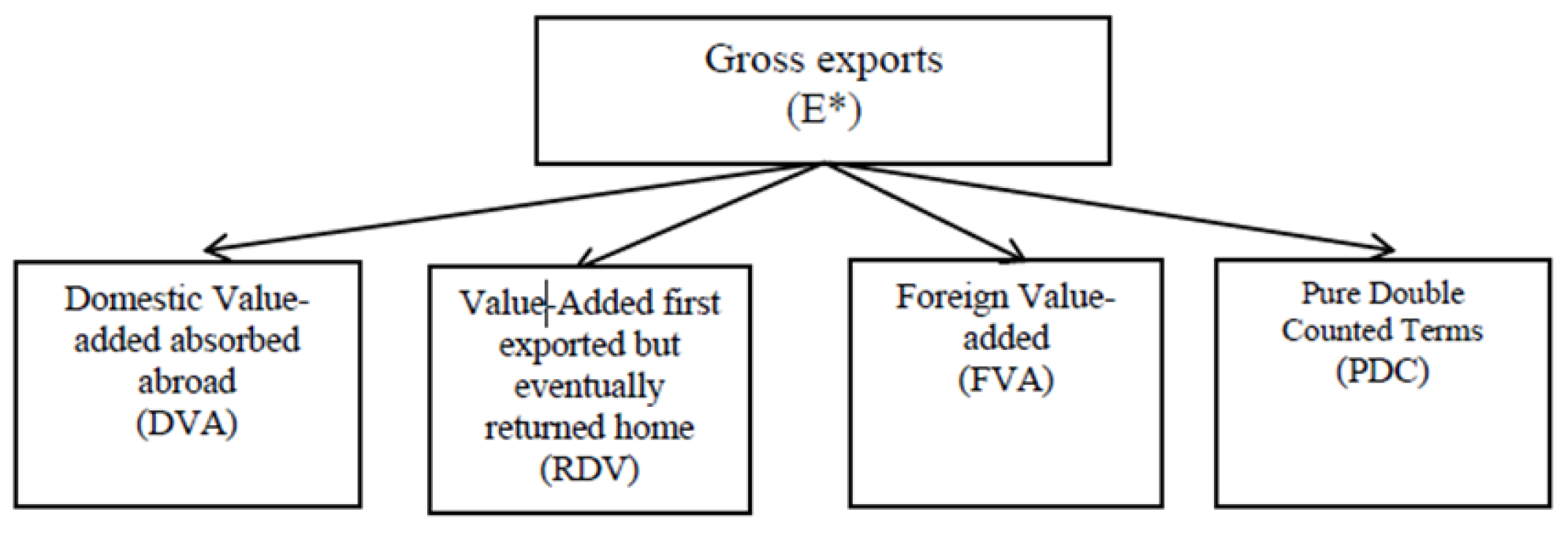
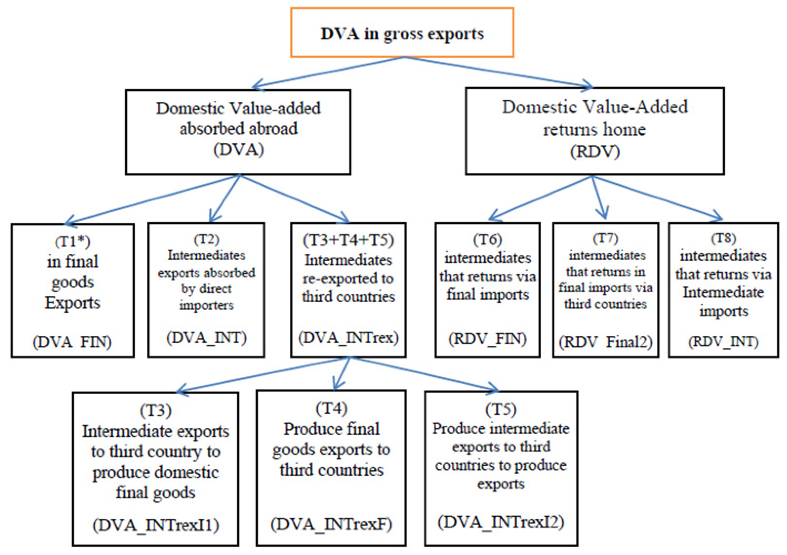
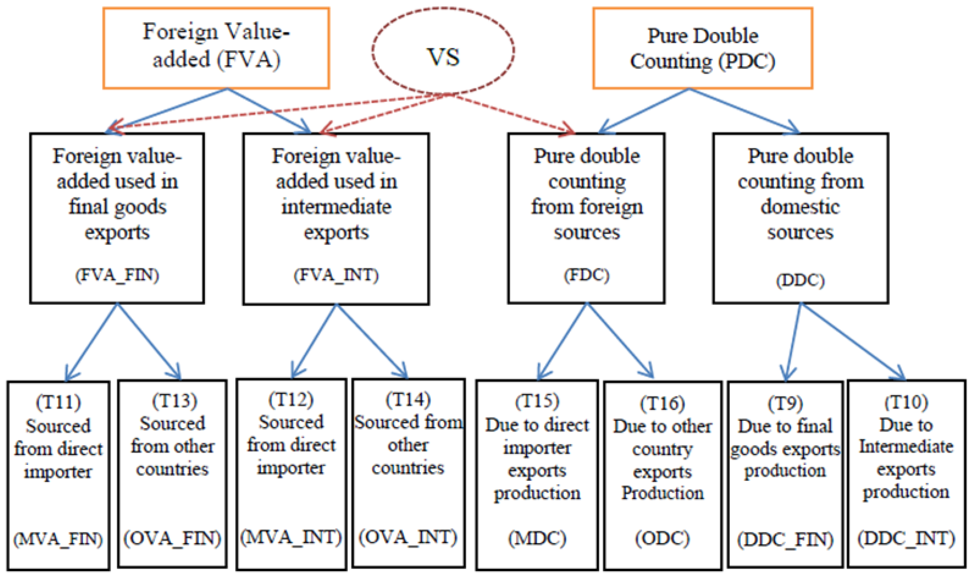
4.1. The Accounting Framework of GVC

GVC is also called “vertical specialization”, and it has many related labels (such as “value chain cutting”, “outsourcing production”, “production non-integration”, “production fragmentation”, “multi-level production”, “product internal specialization”, etc.). [115]. Balassa (1965) proposed in the literature about trade liberalization that, a kind of continuous production processes product is divided into a vertical trade chain, which extends to many countries, and the interconnectivity of this production process is gradually enhanced. Each country focuses on a specific stage in the process of production and adds value according to its comparative advantage. This global division phenomenon is defined as vertical specialization [116]. However, because of data and calculation problems, the research on vertical specialization remained at the case study level until Hummels et al. (2001) defined a narrow concept of vertical specialization and put forward the quantitative index of systematic measurement, which made the measurement of GVC possible. Hummels et al. (2001) defined the value of imported inputs embodied in goods that are exported as vertical specialization (VS) and called the value of exports that are embodied in a second country’s export goods VS1. They provided a formula for computing VS, but no formula for VS1, and pointed out that VS1 is more difficult to measure than VS, as it requires bilateral trade flow data matching the input-output relations [115]. Koopman et al. (2010) deemed that Hummels et al. (2001) provided the first empirical measurements of vertical specialization, but their measurement is valid only in special cases and breaks down when confronted with the multi-country, back-and-forth nature of current global production networks. They pointed out that there are two key assumptions embodied in Hummels’s measurement. First, all intermediate inputs imported should be wholly foreign value-added, with no value-added from itself and returned after processing abroad, and no more than one country can export intermediates. In their model, a country cannot use import intermediates to produce exporting intermediate products. Second, the domestic consumption and exports are produced with the same importing inputs. This assumption is violated when processing exports raise the imported intermediate content of exports relative to domestic use [117]. Relaxing the first assumption, Wang et al. (2009) extended Hummels’s method based on the international input-output model and developed an accounting framework involving multiple countries. Based on the Asian international Input-Output tables, they decomposed value-added in the multinational production chain into the net contribution of each country. They provided formulas for both VS and VS1 and pointed out that Hummels’s measurement is only a special case in certain situations of their framework [118]. Koopman et al. (2008) relaxed the second assumption and proposed a method for computing domestic and foreign value-added under commonly existing processing trade conditions [119]. Koopman et al. (2010) relaxed both assumptions and provided a complete decomposition of gross exports into its value-added components, thus, making it possible to connect trade statistics with SNA standards and construct a quantitative index to assess whether a particular sector in a country is likely located in the upstream or downstream of the global production chain [117]. The concept of vertical specialization in these studies, following the narrow concept of vertical specialization proposed by Hummels et al. (2001), is extended to the global system. For closed economies, IO information can be fully captured in the regional IO table. Under such circumstances, a narrow vertical specialization is only a special case of the new framework. Other studies expand the elements related to vertical specialization and define new indicators for measurement. Daudin et al. (2011) defined VS1* as the exports that, further down the production chain, are embedded in re-imported goods that are either consumed, invested, or used as inputs for final domestic use, namely, the domestic content of invested or consumed imports [120]. Johnson et al. (2012) defined the value-added produced in one country and eventually absorbed in other countries as value-added export (VAX) and used the ratio of VAX to total export (VAX ratio) as the measurement index of value-added in trade (VaiT) [5]. Stehrer et al. (2012) discussed the measurement of TiVA and VaiT, defined TiVA as a country’s direct and indirect value-added embodied in the final foreign consumption, and VaiT as the value-added of total trade flow between two countries [121].

TiVA estimates the value-added embodied in imports, exports and net exports based on the use of final products, while VaiT represents the (net) flows of value-added generated by traditional exports and imports. Koopman et al. (2014) decomposed total exports into nine categories of value-added components and double-counting items, but their decomposition was limited to the national level and did not go deeply into the industrial sector level [6]. Wang et al. (2013) compared the TiVA accounting method with the gross value accounting system from the perspective of gross exports and decomposed total exports into 16 value-added components and double-counting items, thus, realizing the complete decomposition of gross exports. They also pointed out that the VS, VS1, and VS1* indicators only represent part of the components or linear combinations after decomposition [122]. In their work, gross exports can be decomposed into domestic value-added, foreign value-added (FVA), and double-counting items (PDC). Domestic value-added can be further decomposed into domestic value-added absorbed in foreign countries (DVA) and domestic value-added that is exported before finally coming back (RDV), as shown in Figure 1. Furthermore, the domestic value-added of exports can be divided into eight types based on the form of export products, their absorption mode and the form of returned products, as shown in Figure 2. The FVA can be further divided into four parts according to their country of origin and product form, and the PDC can be further divided into four parts according to their source, as shown in Figure 3.

The main estimating formula is as follows:

$$\begin{array}{cc}{E}^{sr}=& \underset{\left(\mathrm{T}1\right)}{\underbrace{{(V^s{B}^{ss})}^{\mathrm{T}}\#Y^{sr}}}+\underset{\left(\mathrm{T}2\right)}{\underbrace{{(V^s{L}^{ss})}^{\mathrm{T}}\#(A^{sr}{B}^{rr}{Y}^{rr})}}+\underset{\left(\mathrm{T}3\right)}{\underbrace{{(V^s{L}^{ss})}^{\mathrm{T}}\#(A^{sr}{\displaystyle \sum _{t\ne s,r}^G{B}^{rt}{Y}^{tt})}}}\hfill \\ & +\underset{(\mathrm{T}4)}{\underbrace{{(V^s{L}^{ss})}^{\mathrm{T}}\#(A^{sr}{B}^{rr}{\displaystyle \sum _{t\ne s,r}^G{Y}^{rt}})}}+\underset{(\mathrm{T}5)}{\underbrace{{(V^s{L}^{ss})}^{\mathrm{T}}\#(A^{sr}{\displaystyle \sum _{t\ne s,r}^G{\displaystyle \sum _{u\ne s,t}^G{B}^{rt}}}{Y}^{tu})}}\hfill \\ & +\underset{(\mathrm{T}6)}{\underbrace{{(V^s{L}^{ss})}^{\mathrm{T}}\#(A^{sr}{B}^{rr}{Y}^{rs})}}+\underset{(\mathrm{T}7)}{\underbrace{{(V^s{L}^{ss})}^{\mathrm{T}}\#(A^{sr}{\displaystyle \sum _{t\ne s,r}^G{B}^{rt}{Y}^{ts})}}}+\underset{(\mathrm{T}8)}{\underbrace{{(V^s{L}^{ss})}^{\mathrm{T}}\#(A^{sr}{B}^{rs}{Y}^{ss})}}\hfill \\ & +\underset{\left(\mathrm{T}9\right)}{\underbrace{{(V^s{L}^{ss})}^{\mathrm{T}}\#(A^{sr}{\displaystyle \sum _{t\ne s,r}^G{B}^{rs}{Y}^{st})}}}+\underset{(\mathrm{T}10)}{\underbrace{{(V^s{B}^{ss}-V^s{L}^{ss})}^{\mathrm{T}}\#(A^{sr}{X}^r)}}\hfill \\ & +\underset{(\mathrm{T}11)}{\underbrace{{(V^r{B}^{rs})}^{\mathrm{T}}\#Y^{sr}}}+\underset{(\mathrm{T}12)}{\underbrace{{(V^r{B}^{rs})}^{\mathrm{T}}\#(A^{sr}{L}^{rr}{Y}^{rr})}}+\underset{(\mathrm{T}13)}{\underbrace{{(V^r{B}^{rs})}^{\mathrm{T}}\#(A^{sr}{L}^{rr}{E}^{r*})}}\hfill \\ & +\underset{(\mathrm{T}14)}{\underbrace{({\displaystyle \sum _{t\ne s,r}^G{V}^t{B}^{ts}{)}^{\mathrm{T}}}\#Y^{sr}}}+\underset{(\mathrm{T}15)}{\underbrace{{({\displaystyle \sum _{t\ne s,r}^G{V}^t}{B}^{ts})}^{\mathrm{T}}\#(A^{sr}{L}^{rr}{Y}^{rr})}}+\underset{(\mathrm{T}16)}{\underbrace{{({\displaystyle \sum _{t\ne s,r}^G{V}^t}{B}^{ts})}^{\mathrm{T}}\#(A^{sr}{L}^{rr}{E}^{r*})}}\hfill \end{array}$$

(1)

The components of the gross export accounting in Figure 1 correspond to each part in Equation (1), thus, gross exports can be completely decomposed. In this formula, E^sr is the export vector that denotes the gross exports of country s to country r. E^r* is the total export of country r. V^s is the value-added coefficient vector of country s, and V^t and V^r denote the similar. B^rs is the Leontief inverse matrix, which is the total requirement matrix that gives the amount of gross output in producing country r required for one unit increase in final demand in country s, and B^ss, B^rr, B^rt, and B^ts have a similar meaning. A^sr is the total input coefficient matrix, giving intermediate use in country r produced in country s. L^ss and L^rr are the local Leontief inverse matrix. “#” is defined as element-wise matrix multiplication operation, for example, when a matrix is multiplied by a n×1 column vector, each row of the matrix is multiplied by the corresponding row of the vector. Previous concepts related to TiVA can be obtained by a linear combination of some components in the decomposition. So far, the measurement of vertical specialization has been incorporated into a unified and compatible framework, and the GVC accounting framework based on TiVA accounting has been improved [123].

4.2. Measurement of GVC

Characterized by the international division of production, GVC’s depth and breadth continuously extend as the level of the international division of labor is gradually refined from the products to the production processes. The specialization of each country is no longer based on the products it produces, but on the production processes consistent with its comparative advantage. In his discussion of the enterprise value chain, Porter (1985) pointed out that the position of each enterprise in the value chain system has an important impact on their competitiveness [113]. Extending to the global level, each country’s participation status in the GVC also has a profound impact on its benefits and competitiveness in international trade. As the accounting framework of the global value chain gradually improves, many scholars have proposed various indicators to measure a country’s participation status in GVC, including physical location (position in the production chain) and economic status (profitability).

In pinpointing the location of GVC, Dietzenbacher (2005) first proposed using average propagation lengths (APLs) to measure the economic distance between sectors. APLs can be interpreted as the measurement of the average number of steps it takes for cost-push in industry i to affect the price of product j, or as the measurement of the average number of steps it takes for demand-pull in industry j to affect the production in sector i [124]. Dietzenbacher et al. (2007) and Inomata (2008) then extended APLs, applying them to an MRIO model [125,126]. Fally (2011) proposed two measurement indexes, including "distance to final consumption" (such as the average number of production stages between production and final consumption) and "average number of production stages embodied in each product", respectively named upstream and downstream indicators by Antras et al. (2012) and Antras et al. (2013). Wang et al (2017) stated that these indicators have two problems. First, these indicators are calculated based on a sector’s total output, which includes not only final goods and services but also intermediate inputs [127,128,129]. Dietzenbacher et al. (2005) and Dietzenbacher et al. (2007) argued that a production chain’s indicators must start from the initial input of a department, such as labor and capital (or value-added), not its total output. Second, "upstream" and "downstream" indicators are not substitutes for each other, and the two indicators may lead to opposite results for the same country/sector [124,125,130].

Aiming at the first question, Su et al. (2015) improved the upstream indicator based on the TiVA accounting framework and calculated the sectoral upstream indicator in 2011 and exporting upstream indicator in 1995–2011 by using world input-output table (WIOT) information for 40 countries and 35 sectors. The results showed that the previous calculation method is indeed flawed [131]. Ni (2016) extended the production stage number concept to the global input-output framework, making a distinction between the domestic stage and international stage [132]. Ye et al. (2015) defined the average value-added propagation lengths (VAPLs) from the perspective of value-added propagation and defined the average VAPLs from forward and backward perspectives [133]. Ni et al. (2016) also extended VAPLs from the angle of value-added propagation from one sector to a final demand sector (point-to-point), one sector to final a demand sector group (point-to-plane), from a sector group to one final demand sector (plane-to-point) and from a sector group to a final demand sector group (plane-to-plane), and pointed out that generalized VAPLs cover various measurements of GVC location in previous studies [134]. Wang et al. (2017) redefined production length as the distance between initial inputs and final products and pointed out that indicators constructed on this basis are more consistent and more in line with economic interpretation, and the average length of the value chain under this definition is always equal to the ratio between the total output value of each part, and the corresponding value-added resulting from it. Moreover, based on the value-added trade accounting framework proposed by Wang et al. (2013) and Koopman et al. (2014), total production length can be decomposed into the pure domestic stage, the direct TiVA stage, and the GVC stage, which comprehensively reflects in-depth transnational production activities. They pointed out that although there are some conceptual differences between production length measurement and location measurement—as long as the production length is defined according to the number of production stages at the bilateral or sectoral level, indicators representing the position of a country/sector in GVC can be constructed by decomposition at various levels [130]. Yan et al. (2018) further expanded this method by decomposing the change in production chain length into the change each industry’s length and the change in the proportion of each industry’s value-added (industrial structure) to calculate the influencing factors of the change in the length of the production chain [135]. Ni (2018) comprehensively reviewed the literature on GVC measurement and pointed out that the definition of generalized VAPL from sector group to final demand sector (plane-to-point) proposed in Ni et al. (2016) was in line with the backward production length (namely, the downstream indicator of the sector) defined in Wang et al. (2017). Ni (2018) also stated that, no matter how and from which perspective the position and length of production is defined, its core is the weighted sum calculation for each stage of the production process, and Wang et al. (2017) has been largely on perfecting to measure macro GVC position [123].

The economic status of GVC has a direct meaning of welfare, and its measurement indicator, which is expressed by the ratio of domestic value-added in exports (DVAR), is relatively uniform. Generally speaking, the higher the DVAR, the more domestic value is added by a country’s per unit exports, and the stronger the country’s profitability in the international division of labor, in other words, the higher its economic status in the international division of labor. The definition of this indicator can also show that the key point of the DVAR index is the exact definition of value-added exports. Johnson et al. (2012) defined value-added exports from the perspective of the final consumption of products as the value that one country’s production adds, which is eventually absorbed by other countries [5].

With the improvement of the TiVA accounting framework, DVAR is being applied at an ever-increasing rate. Zhang et al. (2013) and Luo et al. (2014) used this indicator to evaluate China’s exports [136,137]. Su (2016) also used this index to evaluate China’s provincial exports [138]. In addition to the DVAR indicator, Koopman et al. (2010) constructed a GVC status index to evaluate the status of sectors in country i in the international division of labor, as shown in Equation (2):

$$GV{C}_{-}{\mathrm{Position}}_{ir}=\ln \left(1+\frac{I{V}_{ir}}{E_{ir}}\right)-\ln \left(1+\frac{F{V}_{ir}}{E_{ir}}\right)$$

(2)

where IVir is a domestic intermediate product used by the importing country to produce exports from sector r of country i, and FVir is a foreign intermediate product used in sector r of country i. They believed that the larger the indicator is, the higher this sector’s economic status is in the division of GVC [117]. Wang et al. (2014) also used this indicator to evaluate the international division of labor status of various manufacturing sectors in China [139]. Wang et al. (2015) then constructed the global value chain status index (GS index), as shown in Equation (3):

$$G{S}_{ik}=v{a}_{i,k}+{\displaystyle \sum _{i,j=1}^G{\displaystyle \sum _{k,l=1}^N\frac{d_{ik,jl}{Y}_{j,l}}{Y_{i,k}}G{S}_{j,l}}}$$

(3)

where, GS_i,k represents GS index of sector k in country i, va_i,k represents its direct value-added coefficient, Y_i,k represents its gross output, d_ik,jl represents the direct consumption coefficients of sector l in country j on sector k in country i, and d_ik,jlY_j,l/Y_i,k represents the proportion of the gross output of sector k in country i used as intermediates in the production of sector l in country j. They believed that the economic meaning of the GS index is the value-added range experienced by intermediate products in a specific industry before they become final products, which can reflect the position and value-added capacity of a country’s specific sectors in the GVC [140].

With the gradual improvement of the value-added accounting framework, until Wang et al. (2013) unified the accounting framework of TiVA and realized the complete quantitative decomposition of gross exports, GVC accounting (and description indicators of on the macro level) had been relatively perfected and applied with increasing frequency in the field of international trade. The GVC accounting framework is based on TiVA accounting, and it can not only solve the “double counting” problem present in EEIT calculation based on traditional trade statistics and the complete decomposition framework of gross exports, but it can also provide an important means to clarify the source, destination and transfer path of emissions embodied in ’ country’s exports. Furthermore, it is importance to make the real EEIT situation clear, and to fairly allocate emissions responsibility among countries.

4.3. The Utilization of GVC Theory in Emission Research

Since the GVC accounting framework has not been implemented until recent years, there are relatively few studies of EEIT based on TiVA accounting. The relevant research can be divided into two categories: (1) Recalculating the EEIT based on TiVA statistics and comparing the results with traditional gross value accounting, and (2) analyzing the original source and destination of EEIT in detail based on the GVC accounting framework.

Xiang et al. (2014) re-estimated the embodied emissions of China’s foreign trade from a TiVA perspective and compared them with traditional estimation results, pointing out that there is an overestimation in the traditional trade statistical method [141]. Liu et al. (2015) estimated the embodied emissions of China’s regional value chain by using China’s MRIO table, and Xu et al. (2017) estimated the embodied emissions of China’s foreign trade, which also proved the overestimation in the traditional trade accounting [142,143]. Pan (2017) put forward an analysis framework based on Koopman et al. (2010) to analyze China’s EEIT, which focuses on the analysis of the influence of China’s position and status in the GVC on its EEIT while the emission transfer path was not involved [144]. Ma et al. (2018) re-estimated the emissions embodied in bilateral trade between China and South Korea in 2001~2011 from a TiVA perspective, pointing out that China and South Korea had an economic trade deficit, but a surplus in EEIT [145]. Zhang et al. (2018) re-estimated the emissions embodied in China-Japan trade and pointed out that there is also an emission deficit in China-Japan trade [146]. Yasmeen et al. (2019) calculated various air pollutants in 39 countries from 1995 to 2009 based on TiVA accounting, and based on this, analyzed the impact of trade on the environment through quantitative research [147]. These studies focus on the total accounting of EEIT (or other pollutants), but fail to analyze the path and stages of emission transfer in detail.

Peng et al. (2016) built an MRIO model based on the GTAP database and reallocated EEIT according to the distribution benchmark of the location of final demand, and defines the emission transfer path [148]. Wang et al. (2018) analyzed the transfer of PM_2.5 related emissions in China through three different trade modes (i.e., trade of final products, trade of intermediate products in the final stage of production, domestic value chain and GVC) based on the TiVA decomposition framework, which is consistent with the decomposition framework featured in Koopman et al. (2010) [149]. Meng et al. (2015) based on the TiVA accounting framework established by Koopman et al. (2014) and Wang et al. (2013) and a large number of other EEIT studies, proposed a set of systematic accounting systems to trace emissions in GVC. The technique used in this study has several advantages. It can trace how downstream countries and industrial sectors absorb emissions from the upstream portion of the value chain. It can also trace the emissions caused by final production in the downstream portion of the GVC to upstream countries and industrial sectors. Finally, it can scientifically trace the emissions embodied in export products according to the direction of trade flow, while analyzing the transfer direction and transfer path of embodied emissions [150]. Meng et al. (2016) also used this model to conduct a detailed decomposition of emissions embodied in China’s exports and their transfer paths in the GVC [151]. Zhang et al. (2018) measured regional exports and their embodied pollutants (PM2.5, SO₂, NOx and NMVOC (non-volatile organic compounds of methane)) by applying TiVA accounting to China’s MRIO table, and tracked the export-oriented economic and environmental costs mismatch along with the state of the supply chain area. They deemed that about 56% of the economic benefits induced by China’s exports go to the developed coastal regions, but about 72% of the associated air pollution is mainly caused by the underdeveloped central and western regions [152]. The study is a regional level application of GVC theory, which traces the domestic paths of the embodied emissions (or other pollutants) involved in international trade in various regions within a country clearly but cannot distinguish their specific destinations. Meng et al. (2013) proposed a new IO table compilation method, that attempts to embed China’s domestic regional IO table into the world IO table. In this method, the domestic and international paths of China’s domestic regions can be traced using this new IO table, showing how they participate in the GVC [153]. Because the current trade statistics system is not yet complete, the compilation of this IO table involves a lot of international trade data, and there may be large errors, thus, receiving less attention, and related research has not been fully developed. Using this method, Pei et al. (2018) analyzed the transfer routes of the embodied emissions originating in each region of China through the GVC [154]. Owing to the limited development of the trade statistics system, it is difficult to compile such IO tables. However, just as the international division of labor is further deepening, production fragmentation is growing in depth intra-nationally. GVC participation actually takes place at the regional and even enterprise level. Research combing the GVC and domestic value chain will also become an important research direction, of which studies like Meng et al. (2013) are effective attempts.

Subjected to the slow progress of the GVC accounting framework and global MRIO statistics, research on EEIT from the GVC perspective is a newly arisen issue, so few studies have even attempted to use it. For example, Zhao et al. (2013) and Zhang et al. (2015) distributed the emission responsibilities of upstream sectors to backstream sectors, final consumption sectors and themselves according to the value-added in their productions. A major weakness in their work is that it assumes that the studied sectors form a closed economic system, so only connections between sectors within this system are considered, and connections between this system and external sectors are not [155,156]. As the GVC accounting framework, intra-national trade statistics and global IO database are being perfected, the combination research on the GVC and emission responsibility allocation is coming closer to drawing a clear roadmap of EEIT sources, destinations, and transfer paths, thus, providing a basis for emission responsibility allocation. This combination of research approaches may be an important trend of the domain in the future.

5. Conclusions and Perspectives

5.1. Conclusions

There are two main deficiencies in the existing EEIT research: Firstly, it is difficult to recognize the sources and destinations of emissions embodied in the processing trade, and there is a lack of relative studies. Secondly, current EEIT accounting is based on traditional gross value statistics, which has an increasingly severe “double counting” problem. Results based on current EEIT accounting do not sufficiently show the real EEIT situation among countries, and are, therefore, unable to establish a fair and reasonable mechanism for global emission responsibility allocation.

PBR, CBR, and SR are currently the most common principles for emission responsibility allocation, and among them, CBR is of special concern in recent studies. There are inevitable drawbacks in both PBR and CBR, which assign responsibility to a single subject. SR seems to be more reasonable as it can press producers and consumers to reduce emissions together. Nevertheless, there is a controversy surrounding the weight of distribution and yet no perfect and commonly acceptable standard for its assignment.

GVC accounting is based on TiVA and can solve the “double counting” problem in current EEIT accounting, as well as provide a clear roadmap of EEIT sources, destinations and transfer paths using the decomposition framework of gross exports. GVC theory provides new ways to determine EEIT and its allocation of responsibility, and there are some effective empirical studies.

GVC accounting framework has been improved at the macro level, but it is still a field on the frontier of current research. Therefore, it still has many theoretical and practical obstacles to in-depth study and further study. The main drawback is the faultiness of the current trade statistic system; however, the global input-output database and international trade statistics have been increasingly accurate, meaning empirical analysis and application are predicted to be more extensive.

5.2. Perspectives

As the processing trade accounts more in the gross international trade, the use of TiVA accounting to calculate EEIT, which distinguishes processing and non-processing trade, can provide a detailed analysis of countries’ EEIT and more accurately describe the current global EEIT situation. It helps to compare the national and global emission reduction pressures and targets, and further provide references for formulating and implementing effective emission reduction policies.

It’s of paramount importance to establish a global emission chain according to GVC theory and to then apply GVC measurement to the global emission chain. This helps to analyze the influence of a country’s GVC position and status on EEIT and can provide effective references for relative policy-making and implementation for countries.

The GVC is not only directly supported by the direct exporting regions, but also indirectly supported by other regions that provide intermediate goods and services to these exporting regions. However, in most of the current GVC studies, China participates in GVC as one region. Considering the vastness of China, the economic development, industrial structure, and export structure differ among regions. It’s also essential to embed the regional input-output relationship of China into the global input-output table to analyze the global value chains and global emission chains—such studies help to analyze the performance in the global value chain and global emission chain for each region of China and enhance their competitiveness when participating in global production. Meng et al. (2013) provided a new framework for measuring the domestic linkages to global value chains [157], and more empirical studies are urgently needed.

The economic benefits and environmental costs of products and services are globally scattered, any principle that assigns responsibility to a single subject has its inevitable defects, and SR is a better choice. By decomposing global international trade flow and EEIT to analyze their sources, destinations, and transfer paths, the real economic benefits and emission costs for countries participating in the GVC can be calculated. Based on the specific analysis, we can establish a unified correlation index between benefits and emissions, providing a basis to define the responsibility share between producer and consumer. Thus, it is conducive to the establishment of a fair and unified emission responsibility allocation mechanism, which is expected to make both producers and consumers more enthusiastic and active in reducing emissions.

References

1. IPCC Global Warming of 1.5 °C. 2018. Available online: https://www.ipcc.ch/site/assets/uploads/2018/02/ar4_syr_full_report.pdf (accessed on 20 August 2019).
2. Lenzen, M.; Murray, J. Conceptualising environmental responsibility. Ecol. Econ. 2010, 70, 261–270. [Google Scholar] [CrossRef]
3. Suh, S.; Lenzen, M.; Treloar, G.J.; Hondo, H.; Horvath, A.; Huppes, G.; Jolliet, O.; Klann, U.; Krewitt, W.; Moriguchi, Y.; et al. System Boundary Selection in Life-Cycle Inventories Using Hybrid Approaches. Environ. Sci. Technol. 2004, 38, 657–664. [Google Scholar] [CrossRef] [PubMed]
4. Lu, P.P.; Gong, W.Z. Review on research progress of carbon emissions: Embodied of measurement method in international trade. Rev. Ind. Econ. 2015, 6, 82–90. [Google Scholar]
5. Johnson, R.C.; Noguera, G. Accounting for intermediates: Production sharing and trade in value added. J. Int. Econ. 2012, 86, 224–236. [Google Scholar] [CrossRef] [Green Version]
6. Koopman, R.; Wang, Z.; Wei, S. Tracing Value-Added and Double Counting in Gross Exports. Am. Econ. Rev. 2014, 104, 459–494. [Google Scholar] [CrossRef] [Green Version]
7. Wang, Z.; Wei, S.J.; Zhu, K.F. Gross trade accounting method: Official trade statistics and measurement of the global value chain. Soc. Sci. China 2015, 9, 108–127, 206. [Google Scholar]
8. OECD WTO Note. Trade in Value-Added: Concepts, Methodologies and Challenges (Joint OECD WTO Note). Available online: http://www.oecd.org/sti/ind/49894138.pdf (accessed on 9 April 2020).
9. China TSCI. The Facts and China’s Position on China-US Trade Friction. 2018. Available online: http://www.scio.gov.cn/zfbps/32832/Document/1638292/1638292.html (accessed on 20 August 2019).
10. Andrew, R.; Forgie, V. A three-perspective view of greenhouse gas emission responsibilities in New Zealand. Ecol. Econ. 2008, 68, 194–204. [Google Scholar] [CrossRef]
11. Wei, Y.; Wang, L.; Liao, H.; Wang, K.; Murty, T.; Yan, J. Responsibility accounting in carbon allocation: A global perspective. Appl. Energy 2014, 130, 122–133. [Google Scholar] [CrossRef]
12. Xie, R.; Gao, C.; Zhao, G.; Liu, Y.; Xu, S. Empirical Study of China’s Provincial Carbon Responsibility Sharing: Provincial Value Chain Perspective. Sustainability 2017, 9, 569. [Google Scholar] [CrossRef] [Green Version]
13. Jiang, X.; Chen, Q.; Yang, C. A comparison of producer, consumer and shared responsibility based on a new inter-country input–output table capturing trade heterogeneity. Singap. Econ. Rev. 2018, 63, 295–311. [Google Scholar] [CrossRef]
14. Brown, M.T.; Herendeen, R.A. Embodied energy analysis and EMERGY analysis: A comparative view. Ecol. Econ. 1996, 19, 219–235. [Google Scholar] [CrossRef]
15. Wood, R.; Stadler, K.; Simas, M.; Bulavskaya, T.; Giljum, S.; Lutter, S.; Tukker, A. Growth in Environmental Footprints and Environmental Impacts Embodied in Trade: Resource Efficiency Indicators from EXIOBASE3. J. Ind. Ecol. 2018, 22, 553–564. [Google Scholar] [CrossRef] [Green Version]
16. Tukker, A.; Giljum, S.; Wood, R. Recent Progress in Assessment of Resource Efficiency and Environmental Impacts Embodied in Trade: An Introduction to this Special Issue. J. Ind. Ecol. 2018, 22, 489–501. [Google Scholar] [CrossRef] [Green Version]
17. Sato, M. Embodied carbon in trade: A survey of the empirical literature. J. Econ. Surv. 2014, 28, 831–861. [Google Scholar] [CrossRef]
18. Wiedmann, T. A review of recent multi-region input–output models used for consumption-based emission and resource accounting. Ecol. Econ. 2009, 69, 211–222. [Google Scholar] [CrossRef]
19. Wiedmann, T.; Lenzen, M.; Turner, K.; Barrett, J. Examining the global environmental impact of regional consumption activities—Part 2: Review of input–output models for the assessment of environmental impacts embodied in trade. Ecol. Econ. 2007, 61, 15–26. [Google Scholar] [CrossRef]
20. Peters, G.P.; Minx, J.C.; Weber, C.L.; Edenhofer, O. Growth in emission transfers via international trade from 1990 to 2008. Proc. Natl. Acad. Sci. USA 2011, 108, 8903–8908. [Google Scholar] [CrossRef] [Green Version]
21. Zhang, Z.H.; Zhao, Y.H.; SU, B. Current Situation and Prospect on Embodied Carbon in International Trade: A Perspective from Bibliometrics Based on Literature during 1994~2017. J. Ind. Technol. Econ. 2019, 3, 52–65. [Google Scholar]
22. Leontief, W.W. Quantitative Input and Output Relations in the Economic Systems of the United States. Rev. Econ. Stat. 1936, 18, 105–125. [Google Scholar] [CrossRef] [Green Version]
23. Leontief, W.W. The Structure of the U. S. Economy. Sci. Am. 1965, 212, 25–35. [Google Scholar] [CrossRef]
24. Leontief, W.W. An Alternative to Aggregation in Input-Output Analysis and National Accounts. Rev. Econ. Stat. 1967, 49, 412–419. [Google Scholar] [CrossRef]
25. Schaeffer, R.; De Sa, A.L. The embodiment of carbon associated with Brazilian imports and exports. Energy Convers. Manag. 1996, 37, 955–960. [Google Scholar] [CrossRef]
26. Sánchez-Chóliz, J.; Duarte, R. CO2 emissions embodied in international trade: Evidence for Spain. Energy Policy 2004, 32, 1999–2005. [Google Scholar] [CrossRef]
27. Mongelli, I.; Tassielli, G.; Notarnicola, B. Global warming agreements, international trade and energy/carbon embodiments: An input–output approach to the Italian case. Energy Policy 2006, 34, 88–100. [Google Scholar] [CrossRef]
28. Pan, J.; Phillips, J.; Chen, Y. China’s balance of emissions embodied in trade: Approaches to measurement and allocating international responsibility. Oxf. Rev. Econ. Policy 2008, 24, 354–376. [Google Scholar] [CrossRef] [Green Version]
29. Weber, C.L.; Peters, G.P.; Guan, D.; Hubacek, K. The contribution of Chinese exports to climate change. Energy Policy 2008, 36, 3572–3577. [Google Scholar] [CrossRef] [Green Version]
30. Su, B.; Huang, H.C.; Ang, B.W.; Zhou, P. Input–output analysis of CO2 emissions embodied in trade: The effects of sector aggregation. Energy Econ. 2010, 32, 166–175. [Google Scholar] [CrossRef]
31. Wei, B.; Fang, X.; Wang, Y. The effects of international trade on Chinese carbon emissions. J. Geogr. Sci. 2011, 21, 301–316. [Google Scholar] [CrossRef]
32. Dietzenbacher, E.; Pei, J.; Yang, C. Trade, production fragmentation, and China’s carbon dioxide emissions. J. Environ. Econ. Manag. 2012, 64, 88–101. [Google Scholar] [CrossRef]
33. Liu, Y.; Jayanthakumaran, K.; Neri, F. Who is responsible for the CO2 emissions that China produces? Energy Policy 2013, 62, 1412–1419. [Google Scholar] [CrossRef] [Green Version]
34. Jiang, X.; Liu, Y.; Zhang, J.; Zu, L.; Wang, S.; Green, C. Evaluating the role of international trade in the growth of china’s CO2 emissions. J. Syst. Sci. Complex. 2015, 28, 907–924. [Google Scholar] [CrossRef]
35. Su, B.; Ang, B.W. Input–output analysis of CO2 emissions embodied in trade: Competitive versus non-competitive imports. Energy Policy 2013, 56, 83–87. [Google Scholar] [CrossRef]
36. Lin, B.; Sun, C. Evaluating carbon dioxide emissions in international trade of China. Energy Policy 2010, 38, 613–621. [Google Scholar] [CrossRef]
37. Yunfeng, Y.; Laike, Y. China’s foreign trade and climate change: A case study of CO2 emissions. Energy Policy 2010, 38, 350–356. [Google Scholar] [CrossRef]
38. Shui, B.; Harriss, R.C. The role of CO2 embodiment in US–China trade. Energy Policy 2006, 34, 4063–4068. [Google Scholar] [CrossRef]
39. Li, Y.; Hewitt, C.N. The effect of trade between China and the UK on national and global carbon dioxide emissions. Energy Policy 2008, 36, 1907–1914. [Google Scholar] [CrossRef]
40. Yin, X.P.; Chen., M. CO2 embodied in goods of China-US trade: Analysis and policy implications. China Ind. Econ. 2010, 8, 45–55. [Google Scholar]
41. Zhan, J.; Ye, J. Study on the measurement and influencing factors of embodied carbon emissions in the Sino-US trade. J. Guangdong Univ. Bus. Stud. 2014, 4, 29, 36–42. [Google Scholar]
42. Ding, T.; Ning, Y.; Zhang, Y. The contribution of China’s bilateral trade to global carbon emissions in the context of globalization. Struct. Chang. Econ. Dyn. 2018, 46, 78–88. [Google Scholar] [CrossRef]
43. Ahmad, N.; Wyckoff, A. Carbon Dioxide Emissions Embodied in International Trade of Goods; OECD Publishing: Paris, France, 2003. [Google Scholar]
44. Okamura, A.; Sakurai, N.; Tojo, Y.; Nakano, S.; Suzuki, M.; Yamano, N. The Measurement of CO2 Embodiments in International Trade: Evidence from the Harmonised Input-Output and Bilateral Trade Database, 1st ed.; OECD Publishing: Paris, France, 2009. [Google Scholar]
45. Peters, G.P.; Hertwich, E.G. CO2 Embodied in International Trade with Implications for Global Climate Policy. Environ. Sci. Technol. 2008, 42, 1401–1407. [Google Scholar] [CrossRef] [Green Version]
46. Dong, Y.; Ishikawa, M.; Liu, X.; Wang, C. An analysis of the driving forces of CO2 emissions embodied in Japan–China trade. Energy Policy 2010, 38, 6784–6792. [Google Scholar] [CrossRef]
47. Liu, X.; Ishikawa, M.; Wang, C.; Dong, Y.; Liu, W. Analyses of CO2 emissions embodied in Japan–China trade. Energy Policy 2010, 38, 1510–1518. [Google Scholar] [CrossRef] [Green Version]
48. Ding, T.; Ning, Y.; Zhang, Y. The Contribution of China’s Outward Foreign Direct Investment (OFDI) to the Reduction of Global CO2 Emissions. Sustainability 2017, 9, 741. [Google Scholar] [CrossRef] [Green Version]
49. Weitzela, M.; Ma, T. Emissions embodied in Chinese exports taking into account the special export structure of China. Energy Econ. 2014, 45–52. [Google Scholar] [CrossRef] [Green Version]
50. Du, H.; Liu, H.; Zhu, K.; Zhang, Z. Re-examining the embodied air pollutants in Chinese exports. J. Environ. Manag. 2020, 253, 109709. [Google Scholar] [CrossRef]
51. Ang, B.W.; Liu, F.L. A new energy decomposition method: Perfect in decomposition and consistent in aggregation. Energy 2001, 26, 537–548. [Google Scholar] [CrossRef]
52. Ma, C.; Stern, D.I. China’s changing energy intensity trend: A decomposition analysis. Energy Econ. 2008, 30, 1037–1053. [Google Scholar] [CrossRef] [Green Version]
53. Su, B.; Ang, B.W. Structural decomposition analysis applied to energy and emissions: Some methodological developments. Energy Econ. 2012, 34, 177–188. [Google Scholar] [CrossRef]
54. Xie, S. The driving forces of China’s energy use from 1992 to 2010: An empirical study of input–output and structural decomposition analysis. Energy Policy 2014, 73, 401–415. [Google Scholar] [CrossRef]
55. Su, B.; Ang, B.W.; Li, Y. Input-output and structural decomposition analysis of Singapore’s carbon emissions. Energy Policy 2017, 105, 484–492. [Google Scholar] [CrossRef]
56. Tan, R.; Lin, B. What factors lead to the decline of energy intensity in China’s energy intensive industries? Energy Econ. 2018, 213–221. [Google Scholar] [CrossRef]
57. Wang, H.; Ang, B.W.; Su, B. Assessing drivers of economy-wide energy use and emissions: IDA versus SDA. Energy Policy 2017, 107, 585–599. [Google Scholar] [CrossRef]
58. Rose, A.; Casler, S. Input-Output Structural Decomposition Analysis: A Critical Appraisal. Econ. Syst. Res. 1996, 8, 33–62. [Google Scholar] [CrossRef]
59. Hoekstra, R.V.D.B. Comparing structural and index decomposition analysis. Energy Econ. 2003, 39–64. [Google Scholar] [CrossRef]
60. Lenzen, M. Structural analyses of energy use and carbon emissions - an overview. Econ. Syst. Res. 2016, 28, 119–132. [Google Scholar] [CrossRef]
61. Wang, H.; Ang, B.W. Assessing the role of international trade in global CO2 emissions: An index decomposition analysis approach. Appl. Energy 2018, 218, 146–158. [Google Scholar] [CrossRef]
62. Du, H.; Guo, J.; Mao, G.; Smith, A.M.; Wang, X.; Wang, Y. CO2 emissions embodied in China–US trade: Input–output analysis based on the emergy/dollar ratio. Energy Policy 2011, 39, 5980–5987. [Google Scholar] [CrossRef]
63. Xu, M.; Li, R.; Crittenden, J.C.; Chen, Y. CO2 emissions embodied in China’s exports from 2002 to 2008: A structural decomposition analysis. Energy Policy 2011, 39, 7381–7388. [Google Scholar] [CrossRef]
64. Su, B.; Ang, B.W.; Low, M. Input–output analysis of CO2 emissions embodied in trade and the driving forces: Processing and normal exports. Ecol. Econ. 2013, 88, 119–125. [Google Scholar] [CrossRef]
65. Xu, Y.; Dietzenbacher, E. A structural decomposition analysis of the emissions embodied in trade. Ecol. Econ. 2014, 101, 10–20. [Google Scholar] [CrossRef]
66. Jiang, Y.; Cai, W.; Wan, L.; Wang, C. An index decomposition analysis of China’s interregional embodied carbon flows. J. Clean. Prod. 2015, 88, 289–296. [Google Scholar] [CrossRef]
67. Wu, R.; Geng, Y.; Dong, H.; Tsuyoshi, F.; Xu, T. Changes of CO2 emissions embodied in China-Japan trade: Drivers and implications. J Clean. Prod. 2016, 112, 4151–4158. [Google Scholar] [CrossRef]
68. Su, B.; Thomson, E. China’s carbon emissions embodied in (normal and processing) exports and their driving forces, 2006–2012. Energy Econ. 2016, 59, 414–422. [Google Scholar] [CrossRef]
69. Malik, A.; Lan, J. The role of outsourcing in driving global carbon emissions. Econ. Syst. Res. 2016, 28, 168–182. [Google Scholar] [CrossRef]
70. Zhao, Y.; Liu, Y.; Zhang, Z.; Wang, S.; Li, H.; Ahmad, A. CO2 emissions per value added in exports of China: A comparison with USA based on generalized logarithmic mean Divisia index decomposition. J. Clean. Prod. 2017, 144, 287–298. [Google Scholar] [CrossRef]
71. Mi, Z.; Meng, J.; Guan, D.; Shan, Y.; Song, M.; Wei, Y.; Liu, Z.; Hubacek, K. Chinese CO2 emission flows have reversed since the global financial crisis. Nat. Commun. 2017, 8, 1–10. [Google Scholar] [CrossRef]
72. Davis, S.J.; Caldeira, K. Consumption-based accounting of CO2 emissions. Proc. Natl. Acad. Sci. USA 2010, 107, 5687–5692. [Google Scholar] [CrossRef] [Green Version]
73. Zhou, M.R.; Tan, X.J. A Review of foreign literatures on assigning responsibility for carbon emissions embodied in international trade. J. Int. Trade 2012, 6, 104–114. [Google Scholar]
74. Peng, S.J.; Zhang, W.C.; Wei, R. National carbon emission responsibility. Econ. Res. J. 2016, 51, 137–150. [Google Scholar]
75. Wyckoff, A.W.; Roop, J.M. The embodiment of carbon in imports of manufactured products. Energy Policy 1994, 22, 187–194. [Google Scholar] [CrossRef]
76. Munksgaard, J.; Pedersen, K.A. CO2 accounts for open economies: Producer or consumer responsibility? Energy Policy 2001, 29, 327–334. [Google Scholar] [CrossRef]
77. Ferng, J. Allocating the responsibility of CO2 over-emissions from the perspectives of benefit principle and ecological deficit. Ecol. Econ. 2003, 46, 121–141. [Google Scholar] [CrossRef]
78. Babiker, M.H. Climate change policy, market structure, and carbon leakage. J. Int. Econ. 2005, 65, 421–445. [Google Scholar] [CrossRef]
79. Peters, G.P.; Hertwich, E.G. Post-Kyoto greenhouse gas inventories: Production versus consumption. Clim. Chang. 2008, 86, 51–66. [Google Scholar] [CrossRef]
80. Yu, X.H.; Zhan, X.Y. Review of global carbon emission responsibility division principle. Sci. Technol. Ind. 2016, 16, 5, 137–143. [Google Scholar]
81. Bastianoni, S.; Pulselli, F.M.; Tiezzi, E. The problem of assigning responsibility for greenhouse gas emissions. Ecol. Econ. 2004, 49, 253–257. [Google Scholar] [CrossRef]
82. Rothman, D.S. Environmental Kuznets curves—Real progress or passing the buck A case for consumption-based approaches. Ecol. Econ. 1998, 25, 177–194. [Google Scholar] [CrossRef]
83. Eder, P.; Narodoslawsky, M. What environmental pressures are a region’ industries responsible for? A method of analysis with descriptive indices and input–output models. Ecol. Econ. 1999, 29, 359–374. [Google Scholar] [CrossRef]
84. Parikh, J.K.; Painuly, J.P. Population, Consumption Patterns and Climate Change A Socioeconomic Perspective from the South. Ambio 1994, 23, 434–437. [Google Scholar]
85. Hamilton, C.; Turton, H. Determinants of emissions growth in OECD countries. Energy Policy 2002, 30, 63–71. [Google Scholar] [CrossRef]
86. Lenzen, M.; Pade, L.; Munksgaard, J. CO2 Multipliers in Multi-region Input-Output Models. Econ. Syst. Res. 2004, 16, 391–412. [Google Scholar] [CrossRef]
87. Peters, G.P. From production-based to consumption-based national emission inventories. Ecol. Econ. 2008, 65, 13–23. [Google Scholar] [CrossRef]
88. Fan, G.; Su, M.; Cao, J. An Economic Analysis of Consumption and Carbon Emission Responsibility. Econ. Res. J. 2010, 1, 4–14. [Google Scholar]
89. Zhang, Y.G. Carbon Contents of the Chinese Trade and Their Determinants: An Analysis Based on Non-competitive (Import)Input-output Tables. China Econ. Q. 2010, 9, 1287–1310. [Google Scholar]
90. Zhang, W.F.; Du, Y.S. On the Misalignment of the CO2 Emissions Embodied in China’s Foreign Trade. China Ind. Econ. 2011, 04, 138–147. [Google Scholar]
91. Yan, Y.F.; Zhao, Z.X. Consumption-based Carbon Emissions and Interregional Carbon Spillover Effect: A Comparison between G7, BRIC and Other Countries. J. Int. Trade 2014, 01, 99–107. [Google Scholar]
92. Peng, S.J.; Zhang, W.C.; Sun, C.W. China’s Production-Based and Consumption-Based Carbon Emission and Their Determinants. Econ. Res. J. 2015, 1, 168–182. [Google Scholar]
93. Han, Z.; Chen, Y.H.; Shi, Y. To Measure and Decompose Consumption-Based Carbon Emission from the Perspective of International Final Demand. J. Quant. Tech. Econ. 2018, 35, 7, 114–129. [Google Scholar]
94. Regional Activity Centre for Cleaner Production. Activity Centre for Cleaner Production. A consumption-based approach to greenhouse gas emissions in a global economy—A pilot experiment in the Mediterranean: Case study: Spain. In Regional Activity Centre for Cleaner Production (CP/RAC), Mediterranean Action Plan; United Nations Environment Programme: Barcelona, Spain, 2008. [Google Scholar]
95. Larsen, H.N.; Hertwich, E.G. The case for consumption-based accounting of greenhouse gas emissions to promote local climate action. Environ. Sci. Policy 2009, 12, 791–798. [Google Scholar] [CrossRef]
96. Spangenberg, J.H.; Lorek, S. Environmentally sustainable household consumption: From aggregate environmental pressures to priority fields of action. Ecol. Econ. 2002, 43, 127–140. [Google Scholar] [CrossRef]
97. Cadarso, M.; López, L.; Gómez, N.; Tobarra, M. International trade and shared environmental responsibility by sector. An application to the Spanish economy. Ecol. Econ. 2012, 83, 221–235. [Google Scholar] [CrossRef]
98. Peters, G.P.; Marland, G.; Hertwich, E.G.; Saikku, L.; Rautiainen, A.; Kauppi, P.E. Trade, transport, and sinks extend the carbon dioxide responsibility of countries: An editorial essay. Clim. Chang. 2009, 97, 379–388. [Google Scholar] [CrossRef]
99. Marques, A.; Rodrigues, J.; Lenzen, M.; Domingos, T. Income-based environmental responsibility. Ecol. Econ. 2012, 84, 57–65. [Google Scholar] [CrossRef]
100. Gallego, B.; Lenzen, M. A consistent input–output formulation of shared producer and consumer responsibility. Econ. Syst. Res. 2005, 4, 365–391. [Google Scholar] [CrossRef]
101. Rodrigues, J.; Domingos, T.; Giljum, S.; Schneider, F. Designing an indicator of environmental responsibility. Ecol. Econ. 2006, 59, 256–266. [Google Scholar] [CrossRef]
102. Lenzen, M.; Murray, J.; Sack, F.; Wiedmann, T. Shared producer and consumer responsibility—Theory and practice. Ecol. Econ. 2007, 61, 27–42. [Google Scholar] [CrossRef]
103. Rodrigues, J.F.D.; Domingos, T.M.D.; Marques, A.P.S. Carbon Responsibility and Embodied Emissions: Theory and Measurement; Routledge: London, UK, 2010. [Google Scholar]
104. Heffa Schücking, L.K.Y.L. Bankrolling Climate Change: A Look into the Portfolios of the World’s Largest Banks; Profundo, ungewald, groundWork, Earthlife Africa Johannesburg and Banktrack: Nijmegen, The Netherlands, 2011. [Google Scholar]
105. Liang, S.; Qu, S.; Zhu, Z.; Guan, D.; Xu, M. Income-Based Greenhouse Gas Emissions of Nations. Environ. Sci. Technol 2016, 51, 346–355. [Google Scholar] [CrossRef] [Green Version]
106. Liu, Y.; Chen, S.; Chen, B.; Yang, W. Analysis of CO2 emissions embodied in China’s bilateral trade: A non-competitive import input–output approach. J. Clean. Prod. 2017, 163, S410–S419. [Google Scholar] [CrossRef]
107. Guan, Y.; Huang, G.; Liu, L.; Zhai, M.; Zheng, B. Dynamic analysis of industrial solid waste metabolism at aggregated and disaggregated levels. J. Clean. Prod. 2019, 221, 817–827. [Google Scholar] [CrossRef]
108. Rodrigues, J.; Domingos, T. Consumer and producer environmental responsibility: Comparing two approaches. Ecol. Econ. 2008, 66, 533–546. [Google Scholar] [CrossRef]
109. Kondo, Y.; Moriguchi, Y. CO2 Emissions in Japan: Influences of Imports and Exports. Appl. Energy 1998, 59, 163–174. [Google Scholar] [CrossRef]
110. Chang, N. Sharing responsibility for carbon dioxide emissions: A perspective on border tax adjustments. Energy Policy 2013, 59, 850–856. [Google Scholar] [CrossRef]
111. Fang, K.; Wang, Q. The Academic Research Tendency Study of Carbon Emission Responsibility Allocation Based on Bibliometric Method. Acta Sci. Circumstantiae 2019, 7, 1–23. [Google Scholar]
112. McKerlie, K.; Knight, N.; Thorpe, B. Advancing Extended Producer Responsibility in Canada. J. Clean. Prod. 2006, 14, 616–628. [Google Scholar] [CrossRef]
113. Porter, M.E. Competitive Advantage; Free Press: New York, NY, USA, 1985. [Google Scholar]
114. Bruce Kogut Design global strategies: Profiting from operational flexibility. Sloan Manag. Rev. 1985, 26, 27–38.
115. Hummels, D.; Ishii, J.; Yi, K. The nature and growth of vertical specialization in world trade. J. Int. Econ. 2001, 54, 75–96. [Google Scholar] [CrossRef]
116. Balassa, B. Trade Liberalisation and “Revealed” Comparative Advantage. Manch. Sch. 1965, 33, 99–123. [Google Scholar] [CrossRef]
117. Koopman, R.; Powers, W.; Wang, Z.; Wei, S. Giving Credit Where Credit is Due: Tracing Value Added in Global Value Chains; NBER Working Paper; NBER: Massachusetts, MA, USA, 2010. [Google Scholar]
118. Wang, Z.; Wei, S.; Yi, K. Value Chain in East Asia Production Network—An International Input-Output Based Analysis; USITC Working Paper; Office of Economics, U.S. International Trade Commission: Washinbton, DC, USA, 2009.
119. Koopman, R.; Wang, Z.; Wei, S. How Much of Chinese Exports is Really Made in China? Assessing Domestic Value-Added When Processing Trade is Pervasive; NBER Working Paper; NBER: Massachusetts, MA, USA, 2008. [Google Scholar]
120. Daudin, G.; Rifflart, C.; Schweisguth, D. Who produces for whom in the world economy? Can. J. Econ. Rev. Can. D’economique 2011, 44, 1403–1437. [Google Scholar] [CrossRef] [Green Version]
121. Stehrer, R. Trade in Value Added and the Value Added in Trade; WIOD Working Paper; The Vienna Institute for International Economic Studies: Wien, Austria, 2012. [Google Scholar]
122. Wang, Z.; Wei, S.; Zhu, K. Quantifying International Production Sharing at the Bilateral and Sector Level; NBER Working Paper Series No. w19677; NBER: Massachusetts, MA, USA, 2013. [Google Scholar]
123. Ni, H.F. New Progress in the Theory and Application of Global Value Chain Measurement. J. Zhongnan Univ. Econ. Law 2018, 3, 115–126, 160. [Google Scholar]
124. Erik, D.; Isidoro, R.; Bosma, N.S. Using average propagation lengths to identify production chains in Andalusian Economy. Estud. Econ. Apl. 2005, 23, 405–422. [Google Scholar]
125. Erik, D.; Isidoro, R. Production Chains in an Interregional Framework: Identification by Means of Average Propagation Lengths. Int. Reg. Sci. Rev. 2007, 30, 362–383. [Google Scholar]
126. Inomata, S. A New Measurement for International Fragmentation of the Production Process: An International Input-Output Approach; IDE Discussion Paper, No.175; Institute of Developing Economies, Japan External Trade Organization (JETRO): Chiba, Japan, 2008.
127. Thibault, F. On the Fragmentation of Production in the US; University of Colorado-Boulder: Boulder, CO, USA, 2011. [Google Scholar]
128. Antràs, P.; Chor, D. Organizing the Global Value Chain; NBER Working Paper No. 18163; NBER: Massachusetts, MA, USA, 2012; Available online: http://www.nber.org/papers/w18163 (accessed on 9 April 2020).
129. Pol, A.; Chor, D.; Fally, T.; Hillberry, R. Measuring the Upstreamness of Production and Trade Flows; NBER Working Paper No. 17819; National Bureau of Economic Research: Cambridge, MA, USA, 2012. [Google Scholar]
130. Wang, Z.; Wei, S.J.; Yu, X.D.; Zhu, K.F. Characterizing Global and Regional Manufacturing Value Chains: Stable and Evolving Features; NBER Working Paper; NBER: Massachusetts, MA, USA, 2017. [Google Scholar]
131. Su, Q.Y.; Gao, L.Y. Positions along Global Value Chains and Its Evolution Law. Stat. Res. 2015, 12, 38–45. [Google Scholar]
132. Ni, H.F. Is There Smile Curves of Industry in Global Value Chains. J. Quant. Tech. Econ. 2016, 11, 111–126. [Google Scholar]
133. Ye, M.; Meng, B.; Wei, S. Measuring Smile Curves in Global Value Chains; IDE Discussion Paper, Institute of Developing Economies (IDE-JETRO): Chiba, Japan, 2015.
134. Ni, H.F.; Gong, L.T.; Xia, J.C. The Evolution Path of Production Fragmentation and Its Factors. Manag. World 2016, 4, 10–23. [Google Scholar]
135. Yan, Y.F.; Zhao, Z.X. China’s Embedded Mechanism and Evolution Path in GVC: Based on Production Length Analysis. World Econ. Stud. 2018, 6, 12–22, 135. [Google Scholar]
136. Zhang, J.; Liu, Z.Y.; Liu, Y.C. Measuring the Domestic Value Added in China’s Exports and the Mechanism of Change. Econ. Res. J. 2013, 10, 124–137. [Google Scholar]
137. Luo, C.Y.; Zhang, J. Trade in Value Added: Evidence from China. Econ. Res. J. 2014, 6, 4–17, 43. [Google Scholar]
138. Su, Q.Y. Re-evaluation of China’s Position in International Division from the Dual Perspectives of Export Technological Sophistication and Domestic Value Added. J. Financ. Econ. 2016, 6, 40–51. [Google Scholar]
139. Wang, L.; Sheng, B. China-US Trade in Value-added and Gains from Bilateral Trade in Global Value Chain. J. Financ. Res. 2014, 9, 97–108. [Google Scholar]
140. Wang, L.; Li, H.Y. Research on GVCs Integrating Routes of China’s Manufacturing Industry—Perspectives of Embedding Position and Value-adding Capacity. China Ind. Econ. 2015, 2, 76–88. [Google Scholar]
141. Xiang, S.J.; Wen, T. Re-estimation of the Implicit CO2 Emissions in China’s Foreign Trade from the Perspective of New Value-added Trade Statistics. Int. Econ. Trade Res. 2014, 17–29. [Google Scholar]
142. Liu, H.; Liu, W.; Fan, X.; Liu, Z. Carbon emissions embodied in value added chains in China. J. Clean. Prod. 2015, 103, 362–370. [Google Scholar] [CrossRef]
143. Xu, X.; Mu, M.; Wang, Q. Recalculating CO2 emissions from the perspective of value-added trade: An input-output analysis of China’s trade data. Energy Policy 2017, 107, 158–166. [Google Scholar] [CrossRef]
144. Pan, A. The Effect of GVC Division on Carbon Emission Embodied in China’s Foreign Trade. Int. Econ. Trade Res. 2017, 3, 14–26. [Google Scholar]
145. Ma, J.M.; Zhao, Z.G. Re-Estimation of Bilateral Trade and Embodied Carbon Emissions in Sino-Korea Trade. Ecol. Econ. 2018, 34, 14–17, 30. [Google Scholar]
146. Zhang, B.B.; Li, Y.W. Re-calculation of carbon emissions embodied in China-Japan trade based on the new value-added trade method. Resour. Sci. 2018, 40, 250–261. [Google Scholar]
147. Yasmeen, R.; Li, Y.; Hafeez, M. Tracing the trade–pollution nexus in global value chains: Evidence from air pollution indicators. Environ. Sci. Pollut. Res. 2019, 26, 5221–5233. [Google Scholar] [CrossRef]
148. Peng, S.J.; Yu, L.L. Regional Transfer Effect of Carbon Emission from International Trade in Global Production Network. Econ. Sci. 2016, 5, 58–70. [Google Scholar]
149. Wang, Y.; Bi, F.; Zhang, Z.; Zuo, J.; Zillante, G.; Du, H.; Liu, H.; Li, J. Spatial production fragmentation and PM2.5 related emissions transfer through three different trade patterns within China. J. Clean. Prod. 2018, 195, 703–720. [Google Scholar] [CrossRef]
150. Meng, B.; Glen, P.; Wang, Z. Tracing Greenhouse Gas Emissions in Global Value Chains; Working Paper No. 525; Stanford University: Stanford, CA, USA, 2015. [Google Scholar]
151. Meng, B.; Peters, G.; Wang, Z. Tracing China’s CO2 Emissions in Global Value Chains. J. Environ. Econ. 2016, 1, 10–25. [Google Scholar]
152. Zhang, W.; Wang, F.; Hubacek, K.; Liu, Y.; Wang, J.; Feng, K.; Jiang, L.; Jiang, H.; Zhang, B.; Bi, J. Unequal Exchange of Air Pollution and Economic Benefits Embodied in China’s Exports. Environ. Sci. Technol. 2018, 52, 3888–3898. [Google Scholar] [CrossRef] [PubMed]
153. Meng, B.; Xue, J.; Feng, K.; Guan, D.; Fu, X. China’s inter-regional spillover of carbon emissions and domestic supply chains. Energy Policy 2013, 61, 1305–1321. [Google Scholar] [CrossRef] [Green Version]
154. Pei, J.; Meng, B.; Wang, F.; Xue, J.; Zhao, Z. Production Sharing, Demand Spillovers and CO2 Emissions: The Case of Chinese Regions in Global Value Chains. Singap. Econ. Rev. 2018, 63, 275–293. [Google Scholar] [CrossRef]
155. Zhao, D.T.; Yang, S. Assigning the Shared Carbon Emission Responsibility in International Trade. China Popul. Resour. Environ. 2013, 23, 1–6. [Google Scholar]
156. Zhang, Y.; Tang, H.Y. Research on China’s CO2 Emissions Embodied in Trading and Responsibility Sharing: An Example Measurement from Perspective of Industrial Chain. J. Int. Trade 2015, 4, 148–156. [Google Scholar]
157. Meng, B.; Wang, Z.; Koopman, R. How Are Global Value Chains Fragmented and Extended in China’s Domestic Networks; USITC Working Paper; Office of Economics, U.S. International Trade Commission: Washinbton, DC, USA, 2013.
Figure 1. Gross exports accounting: Major categories. Note: E*can be measured at the country/sector level, as a country aggregate, or as a bilateral/sector or bilateral aggregate.
Sustainability 12 03097 g001
Figure 2. Gross exports accounting: Domestic value-added.
Sustainability 12 03097 g002
Figure 3. Gross exports accounting: Foreign value-added.
Sustainability 12 03097 g003