Exploiting OLTC and BESS Operation Coordinated with Active Network Management in LV Networks

Abstract

The large number of small scale Distributed Energy Resources (DER) such as Electric Vehicles (EVs), rooftop photovoltaic installations and Battery Energy Storage Systems (BESS), installed along distribution networks, poses several challenges related to power quality, efficiency, and reliability. Concurrently, the connection of DER may provide substantial flexibility to the operation of distribution grids and market players such as aggregators. This paper proposes an optimization framework for the energy management and scheduling of operation for Low Voltage (LV) networks assuring both admissible voltage magnitudes and minimized line congestion and voltage unbalances. The proposed tool allows the utilization and coordination of On-Load Tap Changer (OLTC) distribution transformers, BESS, and flexibilities provided by DER. The methodology is framed with a multi-objective three phase unbalanced multi-period AC Optimal Power Flow (MACOPF) solved as a nonlinear optimization problem. The performance of the resulting control scheme is validated on a LV distribution network through multiple case scenarios with high microgeneration and EV integration. The usefulness of the proposed scheme is additionally demonstrated by deriving the most efficient placement and sizing BESS solution based on yearly synthetic load and generation data-set. A techno-economical analysis is also conducted to identify optimal coordination among assets and DER for several objectives.

1. Introduction

Low Voltage (LV) distribution networks used to be a passive segment of the power system, mainly for the supply of consumers; thus, power flows were heading from the bulk transmission points to the distribution grid. Accordingly, from the secondary substation and the downstream connected LV grid, there used to be very limited or an absence of automation for its monitoring and control [1]. In the last decade, there has been a large number of small-scale units, commonly referred to as Distributed Energy Resources (DER), that are getting connected along distribution grids. Several types of DER may be connected such as domestic rooftop Photovoltaics (PV) or generally microgeneration ($\mathsf{\mu }$G) in some cases coupled with Battery Storage Systems (BESS), controllable loads (e.g., Electric Heat Pumps or other smart domestic appliances), and Electric Vehicles (EVs). The extensive integration of DER in the grid may cause several technical challenges on the operation of distribution networks such as voltage problems, branch congestions, and phase unbalances. Despite these technical bottlenecks, DER may be utilized in favor of the grid operation, providing ancillary services and supporting the bulk transmission system and distribution networks [2,3].

The Distribution System Operators (DSOs) are currently adopting practices to enhance the observability and controllability of the distribution grids throughout Advanced Distribution Management Systems (A-DMS), [4]. The active involvement of DER and generally prosumers in the operation of the network is generally referred to active network management, which is regarded to take place utilizing their flexibility. Sources of flexibility may come from several types of DERs that are enabled with temporal shifting of active or reactive power to be consumed or injected into the grid. Such strategies of active participation of consumers in the grid’s operation have gained the interest of utilities for the past few decades by engaging, mainly, industrial consumers through demand side management schemes [5]. Several research works have discussed recently about the Smart Transformers (STs) envisioned as a key element for the controllability of distribution networks in a future context of DER massification [6]. For the smart grid development, more novel advanced control schemes have to be implemented towards the active involvement of DER.

2. Related Works and Contributions

The operational control schemes and energy management applications could be generally classified into several categories according to the communication infrastructure and the data requirement (i.e., deemed necessary to be used). Based on the latter, centralized schemes usually look for solutions not only to resolve technical grid constraints but also to optimize the economical operation of the grid [7,8,9]; local control (or decentralized) techniques may be applied merely relying on droop based rules [10,11] and distributed strategies which are in line with the deployment of local energy communities and transactive energy concepts [12,13,14].

In LV distribution networks, voltage regulation and phase balancing are managed by the DSOs, typically by manual adjustments (offline) of the MV/LV—secondary—transformer which may happen once or twice a year, depending on the seasonal changes in the loads [15]. Alternatively, DSOs act by investing on grid reinforcement measures such as line replacement (i.e., when branch congestions) and manual phase redistribution for phase balancing [16,17]. Considering the stochasticity of both load and generation, the aforementioned practices of manual configuration of tap-positions and grid reconstruction may be inadequate in many cases [18]. Manual controls and simple local controls may be insufficient due to the intermittent nature of $\mathsf{\mu }$G and the stochastic behavior of EV charging. On the other hand, the grid reinforcement may be considered quite effective but still a costly measure for the DSO.

The possibility of utilizing droop capabilities (for active and reactive power control –$P=f\left(V\right)$, $Q=f\left(V\right)$, accordingly) with a smart PV inverter particularly for voltage regulation has extensively been studied in the literature [10,19,20]. The reactive power control is generally a less efficient solution in the LV grid for voltage control due to the high branch ratio R/X (i.e., rather resistive nature of LV distribution lines) compared to Medium Voltage (MV) distribution networks or transmission. Self-consumption is commonly imposed by regulation and legislation lately, to address voltage rise effects during the peak period of PV generation. In several European countries (e.g., Belgium, Denmark, the Netherlands and Greece), residential PV self-consumption measures based on net metering schemes aim at matching the endogenously generated power with local demand [21]. In Germany, there is a cap for active power feed-in at 70% of the installed capacity for all the prosumers with a capacity of less than 30 kWp [22]. Nevertheless, Active Power Curtailment (APC) might not be an economically attractive solution for both DSOs and the prosumers. Therefore, more sophisticated control schemes are proposed exploiting the coordination of $\mathsf{\mu }$G with DSO assets to improve the network’s power quality [23,24].

Several applications have focused their interest on introducing the control of other DER, such as BESS or EVs. Most research applications refer to the coupling of BESS systems with $\mathsf{\mu }$G to firm-up the dispatched power produced from PVs by reducing the mismatches between generation-demand [21,25]. The increased cost of investment has been the main limitation for the extensive deployment of BESS, a fact that is likely expected to change in the current decade according to [26]. Concurrently, several works have lately proposed the utilization of BESS by DSOs—i.e., owned and controlled by the DSO—[27,28] to deliver operational flexibility operation as well as to increase hosting capacity of DER into the grids. Nonetheless, there is very limited BESS utilization by DSO currently due to the in force Directive 2009/72/EC [29], where the unbundling requirements for DSOs do not allow BESS directly owned and controlled by them. As a result, the ever growing number of domestic BESS may undermine the current business model of the electric utilities [30]. The following trend aims to maximize the revenue brought by “smart” consumers that utilize home energy management systems to optimize the local generation and consumption.

The large-scale penetration of EVs that is expected in the current decade will notably increase electricity consumption, during charging periods. Therefore, power flows—including Vehicle-to-Grid (V2G)—grid losses, and voltage profile patterns and generally power quality along the grid will change significantly [31]. These effects may arise the need to reinforce the grid in some locations. Based on the EV charging strategy to be adopted, grid reinforcement may be deterred. Several schemes have been proposed to derive smart charging schedules to ensure safe grid operation [32,33,34,35], while some of those dealing with phase unbalances may be provoked by EVs in the grid. None of the aforementioned works, however, propose any possible coordination of DER amongst them or with DSO assets to optimize cost objectives or the technical operation.

Several industrial prototypes for secondary transformers (Efacec, Reinhausen, Siemens) are equipped with the capability of On-Load Tap Changer (OLTC) [36] for MV/LV transformers. There is relatively limited work dealing with the coordinated operation of OLTC with DER addressed in [30,37,38,39]. In spite of the fact that these works provide the optimal coordination of OLTC with DER, there is no insight for the temporal flexibility that may be delivered by DER between subsequent time slots. Authors in [7] propose a framework for the optimal coordination among several DER and the OLTC, dealing also with the phase balancing constraint. In this work, authors propose efficient linearizations to resort tractable multi-period OPF extending the problem statement in [40]. On the contrary, a three-phase multi-period OPF based on the exact (i.e., nonlinear) AC power flows is proposed in this work, incorporating multiple DER within the operation of the distribution grid.

This paper advances previous works of the authors [41,42]. The main contributions of this paper may be outlined as follows:

• Advances an analytical DMS framework for the energy management and scheduling of operation of unbalanced distribution networks with increased integration of DERs. The tool is capable of deriving control actions and schedules for flexible DER and the OLTC subjected to multiple operational constraints such as congestion management, phase balancing, and voltage regulation. Furthermore, optional objective terms might be opted among the minimization of operational costs or minimization of flexibility activation costs and minimization of active power losses.
• The proposed DMS tool is extended for planning purposes such as to propose efficient sizing and placement of BESS solutions (i.e., distributed or centralized).
• An analytical study is conducted to compare the alternatives among OLTC, BESS, active network management, or their coordinated operation for scenarios with increased DER integration.
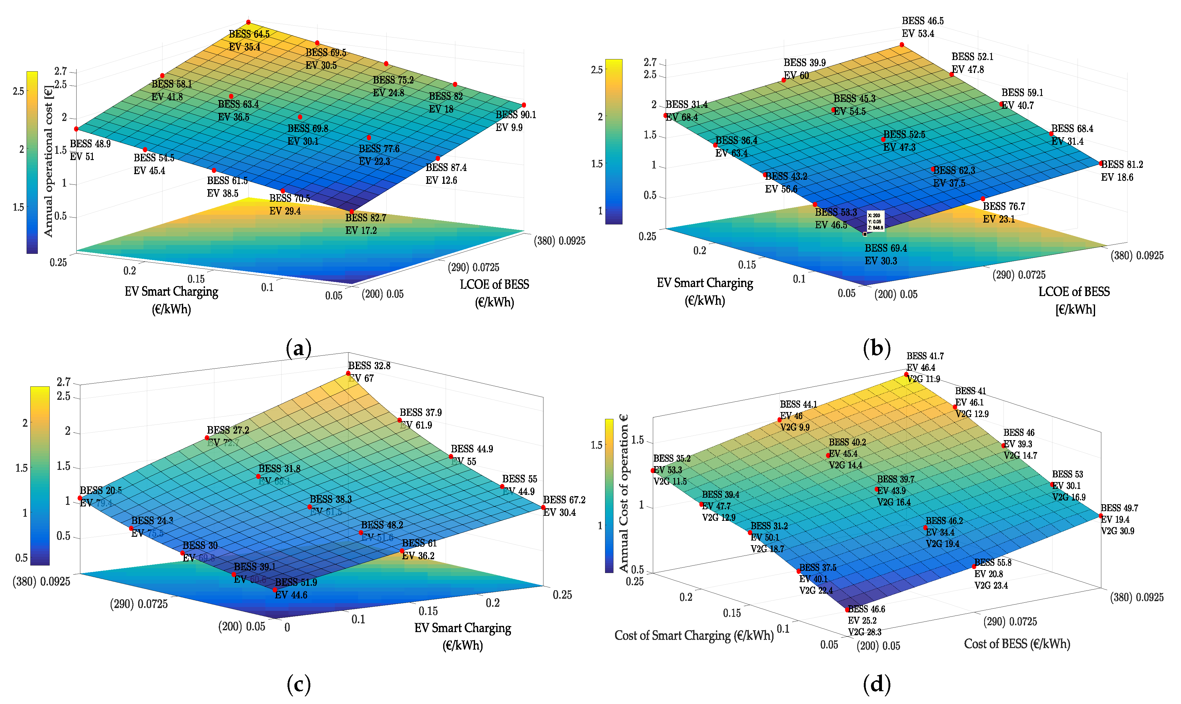
• A sensitivity analysis for coordinated operation between BESS and EVs exploring variable base pricing for the BESS investment and the variable price of EV flexibility.

3. Formulation of Coordinated Active Network Management Tool

This section details the statement of the proposed multi-objective unbalanced Multi-period AC-OPF (MACOPF). The formulation provides a flexible DMS framework for LV unbalanced networks. The main focus is to minimize the DSO/grid’s operation cost; hence, it is essential to minimize DER flexibility activation costs (e.g., minimize the engagement of DER on the operation), the overuse of any DSO assets (e.g., BESS, OLTC), minimize the grid losses as well as to minimize the energy costs by means of the energy imported by the upstream grid. Based on the strategy applied for each type of DER/asset, the optimization strategy (i.e., dispatchable $\mathsf{\mu }$G, definition of EV flexibility, V2G, etc.) may be formulated respectively.

In this study, the LV distribution network is represented as a three-phase four wire unbalanced network with a multi-earthed neutral; this fact allows the application of the Kron’s reduction [43]. More analytical information on the modeling of lines and the transformer may be found in Appendix A. Each time slot is denoted by $\tau \in \mathcal{T}$, where the length of set $\mathcal{T}$ is the horizon of the desired scheduling of operation $H_{\tau }$. Let $x_{g,\tau }$ be the state vector for time slot $\tau$ represented by Equation (1), containing the instant angles and voltage for each bus ($j\in \{1,\dots N_b\}$) and phase ($\varphi \in \mathsf{\Phi }$). The vector of decision variables $u_{\tau }$ consists of active and reactive power for each of the controllable DER ($k\in \{1,\dots N_c\}$) as shown in (2). The voltage angles displacement between adjacent nodes may be considered as constant (commonly less than 10${}^{\circ }$ [40]); thus, the scale of the optimization problem can be reduced significantly. However, angles are analytically defined in this work due to the need of assessing phase balancing constraints:

$$\begin{array}{cc}\hfill x_{g,\tau }& ={\left[\begin{array}{c}\Theta \\ \mathcal{V}\end{array}\right]}_{\tau }\forall \tau \in \mathcal{T},x_{\tau }\in {\mathbb{R}}^{(2\ast 3N_b)},\hfill \end{array}$$

(1)

$$\begin{array}{cc}\hfill u_{\tau }& ={\left[\begin{array}{c}{P}_c\\ Q_c\end{array}\right]}_{\tau }\forall \tau \in \mathcal{T},u_{\tau }\in {\mathbb{R}}^{(2\ast N_c)},\hfill \end{array}$$

(2)

$$\begin{array}{cc}\hfill y_{\tau }& ={\left[\begin{array}{ccccccc}{p}_{ch}& p_{dch}& y_{\pi ,ch}& y_{\pi ,dch}& y_{\mathrm{trip}}& y_{\mathrm{tap}}& {ϵ}_{j,\mathrm{con}}\end{array}\right]}_{\tau }\hfill \end{array}$$

(3)

All of the auxiliary variables, for $\tau$, are contained in the $y_{\tau }$; such variables are involved in the DER or OLTC modeling as well as slackness variables to relax constraints and ensure convergence for any resolution. The sets $\mathcal{N}$ and $\mathcal{J}$ stand for the nodes (each bus has three nodes, one per phase) and the branches of the grid. Let X be the vector that contains stacked the state vectors, the decision variables, and any auxiliary variables defined as $X={[x_1,\dots ,x_{H\tau },y_1,\dots ,y_{H\tau }]}^T$. As explained also in [41], the auxiliary variables are intentionally appended as last elements of vector X to allow the flexible configurations of the stated problems (i.e., eases the calculation of derivatives and the data logging of initial points). To avoid lengthy notation on the problem statement, a symbolic variable ${\mathcal{X}}_{\tau }=(x_{g,\tau },u_{\tau },y_{\tau })$ is defined. The MACOPF is stated in Equation (4a):

$${\displaystyle \underset{u}{min}}{\displaystyle \sum _{\tau =1}^{H_t}}\left[\left\{w_1·{\mathsf{\Pi }}_{\mathit{\tau }}+w_2·{{\mathbf{P}}_{\mathbf{L}}}_{\tau }\right\}\Delta \tau +w_3·{{\mathbf{U}}_{\mathrm{OLTC}}}_{\mathit{\tau }}+w_4·{\mathbf{Tap}}_{\mathit{\tau }}+{\mathsf{\Phi }}_{p,\mathit{\tau }}\right],$$

(4a)

subjected to

$$\begin{array}{ccc}\hfill G_j\left({\mathcal{X}}_{\tau }\right)=0,& \hfill & \hfill \forall j,\tau \in \mathcal{N},\mathcal{T},\end{array}$$

(4b)

$$\begin{array}{ccc}\hfill H_{Sub}\left({\mathcal{X}}_{\tau }\right)\le S_{rated}-{\epsilon }_{sub},& \hfill & \hfill \forall \tau \in \mathcal{T},\end{array}$$

(4c)

$$\begin{array}{ccc}\hfill VU{F}_j\left({\mathcal{X}}_{\tau }\right)\le \overline{\mathrm{VUF}}-{\epsilon }_{\mathrm{VUF}},& \hfill & \hfill \forall i,\tau \in \mathcal{N},\mathcal{T},\end{array}$$

(4d)

$$\begin{array}{ccc}\hfill V_{\min }-{\epsilon }_{{\mathcal{V}}_{j,\tau }}\le v_j\le V_{\max }+{\epsilon }_{{\mathcal{V}}_{j,\tau }},& \hfill & \hfill j,\tau \in \mathcal{N},\mathcal{T},\end{array}$$

(4e)

$$\begin{array}{ccc}\hfill h_{\xi }\left({\mathcal{X}}_{\tau }\right)=0,& \hfill & \hfill \forall \xi ,\tau \in \mathcal{U},\mathcal{T},\end{array}$$

(4f)

$$\begin{array}{ccc}\hfill g_{\xi }\left({\mathcal{X}}_{\tau }\right)\le 0,& \hfill & \hfill \forall \xi ,\tau \in \mathcal{U},\mathcal{T},\end{array}$$

(4g)

where the analytical expression of the objective is the following:

$$\begin{array}{ll}{\mathsf{\Pi }}_{\mathit{\tau }}={\displaystyle \sum _k^{N_b}}\left({\left[c_k\left(\tau \right)\right]}^T·u_{k,\tau }\right)& {\mathcal{O}}_1:\mathrm{flexibility}\mathrm{activation}\mathrm{costs}\\ {{\mathbf{P}}_{\mathbf{L}}}_{\tau }={\displaystyle \sum _{\varphi \in \mathsf{\Phi }}}{\displaystyle \sum _{i\in \mathcal{B}}}\frac{{\left(\Delta V_{\phi ,ij}\right)}^2}{R_{\phi ,ij}}\hfill & {\mathcal{O}}_2:\mathrm{Apparent}\mathrm{power}\mathrm{losses}\\ {{\mathbf{U}}_{\mathrm{OLTC}}}_{\mathit{\tau }}={\displaystyle \sum _{\varphi \in \mathsf{\Phi }}}{\left(V_{\varphi ,ps}\left(\tau \right)-V_{\varphi ,ps}(\tau -1)\right)}^2\hfill & {\mathcal{O}}_3:\mathrm{Penalize}\mathrm{fast}\mathrm{transitions}\mathrm{of}\mathrm{primary}\mathrm{winding}\mathrm{voltage}\\ {\mathbf{Tap}}_{\mathit{\tau }}={\displaystyle \sum _{\varphi \in \mathsf{\Phi }}}{\left(t_{c_{\varphi }}\left(\tau \right)-t_{c_{\varphi }}(\tau -1)\right)}^2\hfill & {\mathcal{O}}_4:\mathrm{Cost}\mathrm{of}\mathrm{tap}\mathrm{operations}\end{array}$$

and vector $c_k\left(\tau \right)$ assigns a price for the utilization of controllable DER or asset k at $\tau$ in €/kWh or €/kVArh. Multiple pricing schemes may be defined, enabling demand–response schemes. The exact form of nonlinear power flow equations is encapsulated with the nonlinear equality constraints in (4b); inequality constraints (4c) is posed to ensure that the MV/LV transformer is not loaded more than the nominal, or may provide a power cap for the LV grid energy management; (4d) inequality constraints stand for the phase balancing requirements; the boxed constraints in (4e) to maintain all nodal voltage within the preset limits. The slackness variables $\epsilon$ in (4c)–(4e) are applied to slightly relax the constraints and reassure the convergence of the optimizer even when the available active measures cannot strictly provide a solution into the feasible space (thus, it is enlarged). The last equality and inequality constraints (4f)–(4g) describe a generalized form pertaining to operational constraints of all controllable assets and DER.

In the objective function in Equation (4a), the term ${\mathsf{\Phi }}_{p,\mathit{\tau }}$ assigns to some of the auxiliary variables a penalty cost. Such penalty costs may be for the relaxation parameters $\epsilon$, as well as some penalties to prohibit the concurrence of charging and discharging as explained more analytically in the BESS model.

The mathematical form of the objective function is a combination of linear ($F_L$) and quadratic ($F_Q$) cost functions. All the quadratic terms in the objective function are encapsulated by the following Equation (5):

$$F\left(X\right)={\displaystyle \sum _{\tau \in \mathcal{T}}}f\left({\mathcal{X}}_{\tau }\right)=F_L+F_Q=c^T·X+\frac{1}{2}{X}^T·H·X,$$

(5)

where $X\in {\mathbb{R}}^{N_X},N_X=H_{\tau }·(n_x+n_y)$ contains all variables of the stated problem, including the auxiliary variables. Variable X can be defined in the following steps, by primarily considering an additional variable u as proposed in [44]. This u variable can be formed by applying a linear transformation $N_T$ and a shift $\widehat{r}$ to the extended set of the optimization variables:

$$r=N_T·X,$$

(6)

$$u=r-\widehat{r},$$

(7)

To enable flexible extension of such costs able to handle scaled linear and quadratic costs as in Equation (4a), each element of the optimizer full set of variables X (let $x_i$) is input as:

$$x_i=\left\{\begin{array}{cc}{m}_i{f}_a(u_i+z_i),& x_i<-z_i\\ 0,& -z_i\le x_i\le z_i\\ m_i{f}_a(u_i+z_i),& x_i>z_i\end{array}\right.$$

(8)

and

$$f_a=\left\{\begin{array}{cc}\alpha ,& \mathrm{if}{d}_i=1\\ {\alpha }^2,& \mathrm{if}{d}_i=2\end{array}\right.$$

(9)

where $z_i$ provides the option to shift the cost function, $m_i$ scales the variable $x_i$ accordingly, and, according to the specified input $d_i$, the cost function may be shaped as linear or quadratic. This formulation is used to structure all the cost functions. The quadratic terms refer to the loss minimization as well as the operational cost functions for OLTC. For instance, the cost formulation: BESS, EV, $\mathsf{\mu }$G, is a piece-wise linear(PWL) function that is incorporated in the optimization framework through cost constrained variables. Further details regarding this mathematical formulation are given in [41].

3.1. Interior-Point Algorithm

The control framework in (4a) evidently presents a large scale nonlinear programming, since its size is dependent on the length of decision variables, which in turn are increased either with finer-grained time resolutions or with longer horizons of scheduling, i.e., $X\in {\mathbb{R}}^{N_X}:N_X=(2\ast 3N_b+2\ast N_c+2\ast N_{BESS}+2\ast N_{EV}+N_{OLTC})·H_{\tau }$. Additionally, the power flows are regarded as nonlinear equality constraints, enumerated as $N_{nonlin}=2\ast 3\ast N_b\ast H_{\tau }$.

The stated MACOPF is addressed using the Interior-Point (IP) primal-dual algorithm. Assume the compact formulation for the stated MACOPF by the set of Equation (10), where the set of variables is denoted by $\mathbf{x}$:

$${\displaystyle \underset{\mathbf{x}}{min}}f\left(\mathbf{x}\right),$$

(10a)

subject to

$$g_E\left(\mathbf{x}\right)=\mathbf{0},$$

(10b)

$$h_I\left(\mathbf{x}\right)\le \mathbf{0},$$

(10c)

$${\mathbf{x}}_{min}\le \mathbf{x}\le {\mathbf{x}}_{max},$$

(10d)

The corresponding Lagrangian function is given by Equation (11):

$$\begin{array}{c}{\mathcal{L}}_p(\mathbf{x},\mathbf{\lambda },\mathbf{\sigma },\mathbf{s}):=f_p\left(\mathbf{x}\right)-{\mathbf{\lambda }}^T{g}_E\left(\mathbf{x}\right)-{\mathbf{\sigma }}^T(h_I\left(\mathbf{x}\right)+\mathbf{s})\hfill \end{array}$$

(11)

where vectors $\mathbf{\lambda }$, $\mathbf{\sigma }$ are the Lagrange multipliers for the corresponding equality ($g_E\left(\mathbf{x}\right)$) and inequality constraints $h_I$ which can be regarded also as equality constraints by the addition of slack variables s, such that $h_I\left(\mathbf{x}\right)-\mathbf{s}=\mathbf{0}$. Thereafter, the augmented objective function for the unconstrained problem (penalty function) $f_p\left(\mathbf{x}\right)$ is defined by Equation (12):

$$\begin{array}{c}{\mathcal{L}}_p(\mathbf{x},\mathbf{\lambda },\mathbf{\sigma },\mathbf{s}):=f_p\left(\mathbf{x}\right)-{\mathbf{\lambda }}^T{g}_E\left(\mathbf{x}\right)-{\mathbf{\sigma }}^T(h_I\left(\mathbf{x}\right)+\mathbf{s})\iff \\ \begin{array}{c}\hfill {\mathcal{L}}_p(\mathbf{x},\mathbf{\lambda },\mathbf{\sigma },\mathbf{s})=f\left(\mathbf{x}\right)-{\mu }^{\left(k\right)}{\displaystyle \sum _{j=1}^{N_x}}\ell n(x_j-x_{j,min})-{\mu }^{\left(k\right)}{\displaystyle \sum _{j=1}^{N_x}}\ell n(x_{j,max}-x_j)-\\ \hfill {\mu }^{\left(k\right)}{\displaystyle \sum _{j=1}^{N_{ineq}}}\ell n\left(s_j\right)-{\mathbf{\lambda }}^T{g}_E\left(\mathbf{x}\right)-{\mathbf{\sigma }}^T(h_I\left(\mathbf{x}\right)+\mathbf{s}),\end{array}\end{array}$$

(12)

where ${\mu }^{\left(k\right)}$ stands for the logarithmic barrier parameter per iteration k. The latter is forced to monotonically reduce to 0 as iteration progresses by the minimizer.

The exact formulation of the non-convex nonlinear power flow equality constraints inflicts the certification of the second-order KKT conditions regarding local optimality of one point-solution $p^{*}$. An analytical description for the first and second order KKT conditions may be found in [45]. As per [41], particular computational techniques are proposed to remedy the singularities of the Jacobian matrix (caused by the inter-temporal dependencies of DER) which is necessary to be assessed along with the Hessian one, for the iterative process of the IP algorithm. Based on the MACOPF structure, efficient explicit calculations (exploiting sparsities) of the Jacobian and Hessian matrices are input in the optimizer not only to accelerate the convergence, but also to avoid faulty solution due to the singular Jacobian. A database is used to procure initial points ($X_0$) to the optimizer from past resolutions of the problem, as well as to acquire historical data regarding load and weather forecasts if they are not currently available.

3.2. Multi-Objective MACOPF Treated with a Weighted Sum Method

As presented in the problem statement, MACOPF is clearly a multi-objective optimization problem. The discipline of Pareto needs to be introduced hereby, which is posed to ensure that none of the objectives can be further improved in the search space without any major impact on the objective function. There exist several methods to support the decision maker, but, in practice, the most commonly used one is the weighted sum method; this recommends the scaling (i.e., ${\psi }_i$) and the multiplication of all the objectives with a weighting factor (i.e., $w_i$) as follows:

$$F\left(X\right)={\displaystyle \sum _i^k}{w}_i·O_i\left(X\right)\frac{1}{{\psi }_i},\mathrm{such}\mathrm{that}\left\{\begin{array}{c}{\displaystyle {\sum }_i^k}{w}_i=1,\mathbf{w}\ge \mathbf{0},\mathbf{w}={[w_1,\dots ,w_k]}^T\\ {\psi }_i=max\left(O_i\right)\end{array}\right.$$

(13)

The scaling of each objective term is critical to balance their impact by balancing their order of magnitude on the aggregated objective function but is often disregarded leading to mistaken and overestimated efficient points.

3.3. Grid Constraints

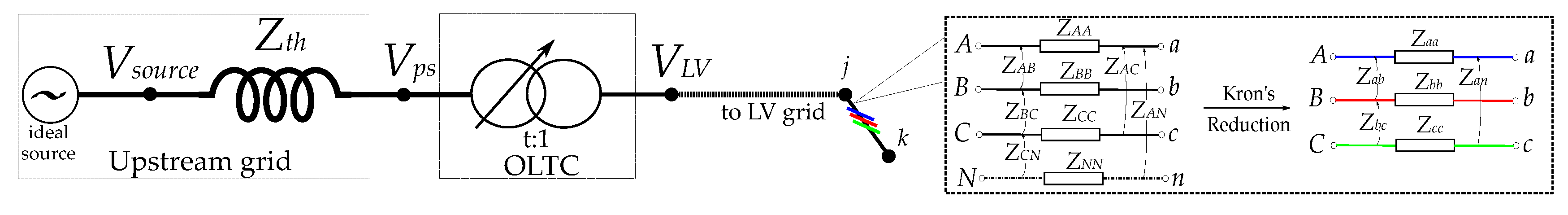
3.3.1. Power Flows

The nonlinear power flows equations, at time instant $\tau$, are formed by Equation (14), expressed as a function of phasor nodal voltage, injection from loads and the DER injection in complex form; essentially imposing that the mismatch between nodal injections and the injection from loads and DER is zero:

$$\begin{array}{c}G\left({\mathcal{X}}_{\tau }\right)=S_{\mathrm{nodal}}\left({\mathcal{X}}_{\tau }\right)+S_{\mathrm{load}}\left({\mathcal{X}}_{\tau }\right)-C_p·S_{\mathrm{DER}}\left({\mathcal{X}}_{\tau }\right)=\mathbf{0}\\ S_{\mathrm{nodal}}\left({\mathcal{X}}_{\tau }\right)=\left[V_{\tau }\right]Y_{\mathrm{bus}}{V}_{\tau }^{*}\end{array}$$

(14)

where the $S_{\mathrm{load}}\in {\mathbb{C}}^{3N_b}$ vector contains the complex loads for all buses of the system; $S_{\mathrm{DER}}\in {\mathbb{C}}^{N_c}$ the DER injections or consumptions. The sparse matrix $C_p\in {\mathbb{N}}^{3N_b\times N_c}$ is defined to map the DER net injections to the $3N_b$ nodes. Any $(i,j)$ element of $C_p$ is zero, whereas it is one if generator j is located in bus i.

3.3.2. Voltage Unbalances

It is important to account for voltage unbalances particularly in LV grids, which inherently present unbalance nature. The integration of single phase DER may lead to much higher unbalances. The Voltage Unbalance Factor (VUF) has several definitions; however, EN 50160 standards make use of the sequence components as in Equation (15), [18]:

$${\mathrm{VUF}}_j[\%]=\frac{|{\upsilon }_{2,j}|}{|{\upsilon }_{1,j}|}·100\%\approx \left|{\upsilon }_{2,j}\right|·100\%,$$

(15)

where ${\upsilon }_{1,j},{\upsilon }_{2,j}$ are positive and negative sequence components, respectively. Obviously, the technical constraints for unbalances present a non-convex nature. Nonetheless, the phase balancing constraint can be easily convexified by the accurate approximation that the magnitude of positive sequence components are closely to 1 p.u. as per [46]. For a node j, the phase balancing constraint is given by Equation (16):

$$\begin{array}{cc}{\mathrm{VUF}}_{j,\tau }-{\epsilon }_{{\mathrm{VUF}}_j}\le 2\%& \forall j\in \mathcal{N},\tau \in \mathcal{T},\end{array}$$

(16)

${\epsilon }_{{\mathrm{VUF}}_j}\le 0$ is an auxiliary variable relaxing the balancing constraint and ensure convergence of MACOPF.

3.3.3. Line Congestion Management

The connection of several EVs along the distribution feeder may increase the peak load profile leading to line congestions. The technical constraint to manage the branch currents is applied at each phase. Let $I_b\left(\tau \right)\in {\mathbb{C}}^{3·3·N_b}$ represent the line currents for $\tau$ slot. Exploiting the definition of the Bus-Injection to Branch-Current (BIBC) matrix as proposed in [47], the phase currents at each branch can be derived from Equation (17):

$$\begin{array}{cccc}{I}_{b_{\tau }}& =& \mathbf{BIBC}·I_{\tau }& \hfill \iff \\ & =& \mathbf{BIBC}·\left(Y_{bus}{V}_{\tau }\right)& \hfill \iff \\ & =& Y_m·V_{\tau },\end{array}$$

(17)

where $Y_m$ represents the modified admittance matrix that maps the nodal current injection vector to the respective branch current injection. The group of nonlinear inequality constraints provided in (18) are posed to ensure line congestion management. The analytical contribution of these constraints into the Jacobian and Hessian is input to the optimizer and is indicatively formulated in Appendix B:

$$\begin{array}{cc}{\mathrm{I}}_{j,\tau }-{\epsilon }_{\mathrm{L}}\le \overline{I_j},& \forall j\in \mathcal{J},\tau \in \mathcal{T}.\end{array}$$

(18)

3.4. OLTC and DER Operational Model

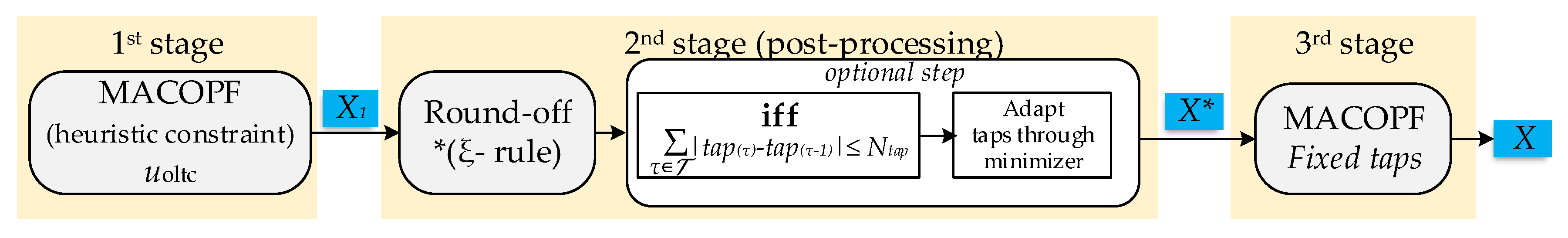
3.4.1. On-Load Tap Changer (OLTC) Model

The OLTC mechanism is considered to be connected at the primary winding of the MV/LV transformer. The primary side is connected through a branch line to the slack bus through a fictitious line impedance (i.e., Z-Thevenin) representing this way the upstream connected MV distribution network, as represented in Figure 1. The incorporation of the OLTC introduces discrete decision variables to determine the tap-positioning at each time step of the horizon. This would resort the MACOPF’s formulation to a Mixed-Integer Nonlinear (MINLP), which is generally classified as an NP-hard problem. The MINLP—especially non-convex problems—are characterized by the challenge of handling the nonlinearities in addition to the combinatorial nature posed by integer decision variables [48]. The continuous relaxation of non-convex MINLP is itself a global optimization problem, thus likely to be NP-hard [49]. In the literature, some approaches have been proposed to treat the discrete nature of tap positions by introducing continuous decision variables as in [38,39,50]. Nevertheless, none of these works couple the stages among them and subsequent time slots (i.e., multi-period optimization) or provide the option to follow any technical limitations as a maximum number of tap changes.

A three-stage resolution is hereby proposed to avoid the introduction of integer variables. In the first stage, the tap changer decision variables are treated as a continuous set $[{\displaystyle \underline{t_{p_a}}},\overline{t_{p_a}}]$. Those decision variables are tracked with heuristic variables that follow the tangent between two-subsequent time slots. The algorithmic diagram of the proposed scheme for the OLTC is illustrated in Figure 2. The corresponding mathematical expressions that connect the tap-positioning decision variables with primary and secondary winding voltage are in Equation (19):

$$\begin{array}{cc}{V}_{LV}=V_{ps}-\Delta s·t_{p_{\varphi }},& \forall \tau ,\varphi \in \mathcal{T},\mathsf{\Phi }\end{array}$$

(19)

where $V_{LV},V_{ps}$ are the voltage magnitudes on secondary and primary winding accordingly and $\Delta s$ is the % resolution of tap-step $t_{p_{\varphi }}$. The constraints have to be applied to all phases since many OLTC provide the option to have different tap-position per phase, yet their control is mechanically coupled to shift them all simultaneously.

The post-processing routine on the second stage lies on the round-off rule described in Algorithm 1. According to this algorithm, the continuous tap-position set is projected to the closest integer variable, whereas a tangent rule is used to enhance the algorithm and avoid excessive tap changes.

Algorithm 1: OLTC round-off $\xi$—rule based on [50]; in this study, $\xi =0.5$.

An optional scheme is included within the second stage relying on a minimizer to adapt the decision taken regarding the tap-position in case of particular technical limitations regarding the daily number of tap changes. This optimizer is set in Equations (20) and (21):

$${\displaystyle \underset{u_d}{min}}{\displaystyle \sum _{\tau }}{\left(u_d\left(\tau \right)-ta{p}_{\tau }\right)}^2$$

(20)

such that

$${\displaystyle \sum _{\tau }}\parallel u_d\left(\tau \right)-u_d(\tau -1)\parallel \le \overline{\Delta tap}.$$

(21)

The optimizer targets to reduce the distance between vectors $u_d\left(\tau \right)$ and $ta{p}_{\tau }$, such that the maximum number of tap-positioning posed for the horizon of the optimization—$\overline{\Delta tap}$. This formulation clearly presents a quadratic function with non-convex constraints. The problem is resolved by using a state-of-the art optimizer called NOMADS [51]. This solver implements a Mesh Adaptive Direct Search algorithm (MADS), which is capable of dealing with non-smooth objective functions and constraints since it resorts to black-box optimization, avoiding the evaluation of costly derivatives.

The post-processing of second stage outputs the discrete tap-positions, which compose inputs for the third stage. The final operational decisions are decided in the third stage where any additional control actions may be determined. The vector $X^{*}$ contains control actions derived from the first stage extracting the OLTC decision variables, and this is then used as an initial point for the last MACOPF resolution.

The characteristics of the OLTC equipment used for this case study are given in

Table 1. On-Load Tap Changer technical and economical parameters [30].

Investment cost (€)	${\mathit{c}}_{\mathit{i}\mathit{n}\mathit{v}}$	7.000
Step Voltage (%)	$\Delta s$	(up to 3) hereby constant at 2
Min/Max tap-position	${\displaystyle \underline{tap}}/\overline{tap}$	(up to $\pm 9$)$\pm 2$
Min/Max voltage (p.u.)	${\displaystyle \underline{V_{ps}}}/\overline{V_{ps}}$	1.1/0.9
Maintanance-free operations	$N_{oltc}$	700.000
Approximated Cost per Tap (€)	$c_{tap}$	0.01

. This equipment may be installed to retrofit an existing transformer, adding the OLTC capability.

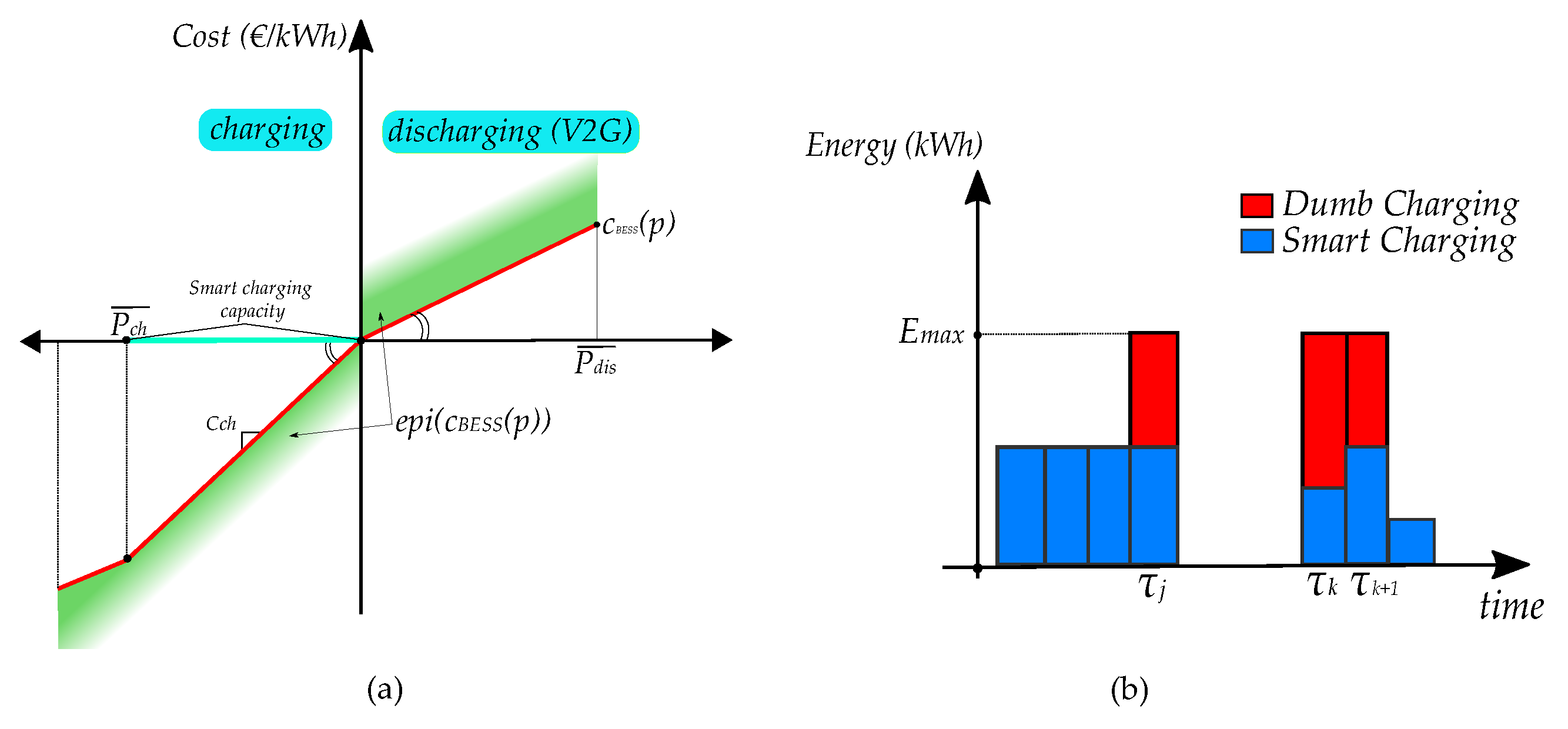
3.4.2. Battery Energy Storage System (BESS)

The BESS model is a first order model, where two distinct auxiliary variables participate in the BESS state equations and operational constraints—one for the discharging $p_{dch}\ge 0$, $p_{dch}\in {\mathbb{R}}_{+}$, while the charging mode $p_{ch}\le 0$, $p_{ch}\in {\mathbb{R}}_{-}$. Any losses occur in each mode of operation are associated with charging and discharging efficiencies (${\eta }_{ch},{\eta }_{dch}$). ${\mathcal{E}}_0$ is defined the initial (i.e., $\tau$ = 0) stored energy at the BESS. The remaining stored energy of a BESS at one time step $\tau$ can be calculated by Equation (22), which clearly bundles the instant energy state with the former one:

$$\begin{array}{cc}\mathcal{E}\left(\tau \right)=\mathcal{E}(\tau -1)-\Delta \tau \left[\begin{array}{cc}{\eta }_{ch}& \frac{1}{{\eta }_{dch}}\end{array}\right]p\left(\tau \right),& \mathrm{where}p\left(\tau \right)=\left[\begin{array}{c}{p}_{ch}\left(\tau \right)\\ p_{dch}\left(\tau \right)\end{array}\right].\end{array}$$

(22)

Within the proposed optimization framework and the subsequent participation of BESSs in the power flow equations (i.e., in $S_{\mathrm{DER}}$), a primary decision variable per BESS defines the scalar variable for active power injections $P_{BESS}$:

$$\begin{array}{cc}\hfill P_{BESS}\left(\tau \right)& =p_{ch}\left(\tau \right)+p_{ch}\left(\tau \right),\hfill \end{array}$$

(23a)

$$\begin{array}{cc}\hfill \overline{p_{ch}}& \le p_{ch}\left(\tau \right)\le 0,\hfill \end{array}$$

(23b)

$$\begin{array}{cc}\hfill 0& \le p_{dch}\left(\tau \right)\le \overline{p_{dch}},\hfill \end{array}$$

(23c)

$$\begin{array}{cc}\hfill {\displaystyle \underline{SoC}}& \le SoC\left(\tau \right)\le \overline{SoC},\hfill \end{array}$$

(23d)

$$\begin{array}{cc}\hfill SOC\left(\tau \right)& =\frac{\mathcal{E}\left(\tau \right)}{{\mathcal{E}}_{rated}}\hfill \end{array}$$

(23e)

$$\begin{array}{cc}\hfill \mathcal{E}\left(0\right)& =\mathcal{E}\left(H_{\tau }\right).\hfill \end{array}$$

(23f)

The constraints (23a)–(23e) are settled $\forall \tau \in \mathcal{T}$. The constraints (23b)–(23d) limit the maximum charging and discharging power as well as the minimum and maximum State-of-Charge (SoC)—defined in Equation (23e)—according to the BESS’s technology and characteristics. The last constraint (23f) imposes that BESS’s ending energy state should be equal to the initial stored energy; thus, the BESS does not get fully discharged.

To avoid simultaneous charging and discharging of the BESS, a penalty cost is assigned with each auxiliary decision variables $p_{ch},p_{dch}$, both of which should be greater—at least one order—than the cost of use of BESS $\left(c_{BESS}\right)$ itself, i.e., $P_{BESS}$.

Based on the European Commission’s study in [26], where several scenarios for Li-ion BESS costs are concerned depending on different market growth indexes,

Table 2. BESS technical consideration based on the data presented on [26] for energy-designed BESS.

	2025 (reference year)
Price (euro/kWh) *(includes costs of investment)	290
Cycles DoD at 80% in lifetime	5000
LCOE calculation (€/kWh)	0.0725

presents the selected characteristics for BESS used in this study. A base price is selected for the year 2025, assuming a moderate adoption of Li-ion BESS by the market. The Levelized Cost of Energy (LCOE) for BESS is also calculated to assign it with the operational costs.

3.4.3. Electric Vehicles

The same mathematical formulations as the BESS’s are settled to simulate the EV operation and technical constraints, with the difference that, in the energy state Equation (22), a term $A_{\tau }=y_{\mathrm{trip}}\left(\tau \right)·E_{\mathrm{tr}}\left(\tau \right)$ is deducted whenever there is a trip occurrence. The variable ${\left[y_{trip}\right]}_{n_{tr}\times H_{\tau }}$ captures the temporal occurrence of a trip combined with the energy consumed $E_{tr}$ along that period. The variable $n_{tr}$ simply refers to the expected number of trips per EV. The combination of those variables creates a mapping of flexibilities (i.e., to charge or discharge based on EVs’ availability, when not used). The Vehicle-to-Grid (V2G) may be considered as an additional mode of operation for the EVs, described by the discharging decision variable.

One can define the energy state of an EV at time period $\tau$ through ${\mathcal{E}}_{EV}(·)\in \mathbb{R}$ that is temporally coupled with the prior period’s energy state and the decision of charging/discharging set-point. For one EV${}_j$, the energy state equation (22) can be recasted in a matrix format (Equation (24)) towards evolution of time as a linear combination of the initial stored energy ${\mathbf{E}}_{\mathrm{EV}}^j={[{\mathcal{E}}_{EV}^j\left(0\right),\cdots ,{\mathcal{E}}_{EV}^j\left(H_{\tau }\right)]}^T$, representing all energy states:

$${\mathbf{E}}_{\mathrm{EV}}^j=\left[\begin{array}{c}I\\ ⋮\\ I\end{array}\right]{\mathcal{E}}_0^j+\left[\begin{array}{ccc}\mathsf{\Lambda }& & \mathbf{0}\\ ⋮& \ddots \\ \mathsf{\Lambda }& \cdots & \mathsf{\Lambda }\end{array}\right]\left[\begin{array}{c}{p}_{\mathrm{EV}}^j\left(1\right)\\ ⋮\\ p_{\mathrm{EV}}^j\left(H_{\tau }\right)\end{array}\right]-{\mathbf{y}}_{\mathrm{trip}}^j·{\mathbf{E}}_{\mathrm{tr}}^j,$$

(24)

where $\mathsf{\Lambda }=\left[\mathrm{diag}\left\{n_{dch}\right\}\mathrm{diag}\{1/n_{ch}\}\right]·\Delta \tau$.

The EVs are modeled to emulate realistic behavior, using a mobility routine as explained analytically in [41]. Further assumptions and details about the EVs are given in Section 4, particularly in regard to the consideration of mobility model and habit of trips. The flexible use of smart charging operation is illustrated in Figure 3b, where some charging energy slots are shifted at later hours. In Figure 3a, the cost function definition is illustrated, where the dumb charging is added on the objective function as a negative cost (i.e., profit), whereas the decision to use smart charging decreases proportionally this profit. The cost function is deployed as a piecewise linear function with a CCV. Note that, for periods when no dumb charging does occur, a V (not purely symmetric since use of V2G is considered more expensive) cost function is considered with its vertex at (0,0).

3.5. Optimal Sizing and Placement of BESS

The optimal sizing and placement of the BESS is hereby derived using an extended formulation of MACOPF as presented in (25):

$${\displaystyle \underset{u,z_j}{min}}\left(w_1·O_1+w_2·O_2\right)+w_{\mathrm{plan}}·{\displaystyle \sum _{j\in \mathcal{D}}}{z}_j$$

(25)

subject to:

$$\begin{array}{ccc}k·z_j& \le p_{ch}\left(\tau \right)& \le 0,\\ 0& \le p_{dch}\left(\tau \right)& \le k·z_j,\\ {\displaystyle \underline{\eta }}\frac{{\mathcal{E}}_j\left(\tau \right)}{z_j}& \le SoC\left(\tau \right)& \le \overline{\eta }\frac{{\mathcal{E}}_j\left(\tau \right)}{z_j}.\end{array}$$

(26)

Variable $z_j$ is added referring to the sizing of the BESS to be installed and the set $\mathcal{D}$ contains all candidate nodes for the investment of a single BESS owned by the DSO. Accordingly, the cost associated with the investment is added on the objective function. The c-rating of the BESS is denoted with k, and the under investment BESS is considered to be a three-phase system. The parameters ${\displaystyle \underline{\eta }},\overline{\eta }$ define the technical parameters for the minimum and maximum SoC for the technology of the BESS to be invested.

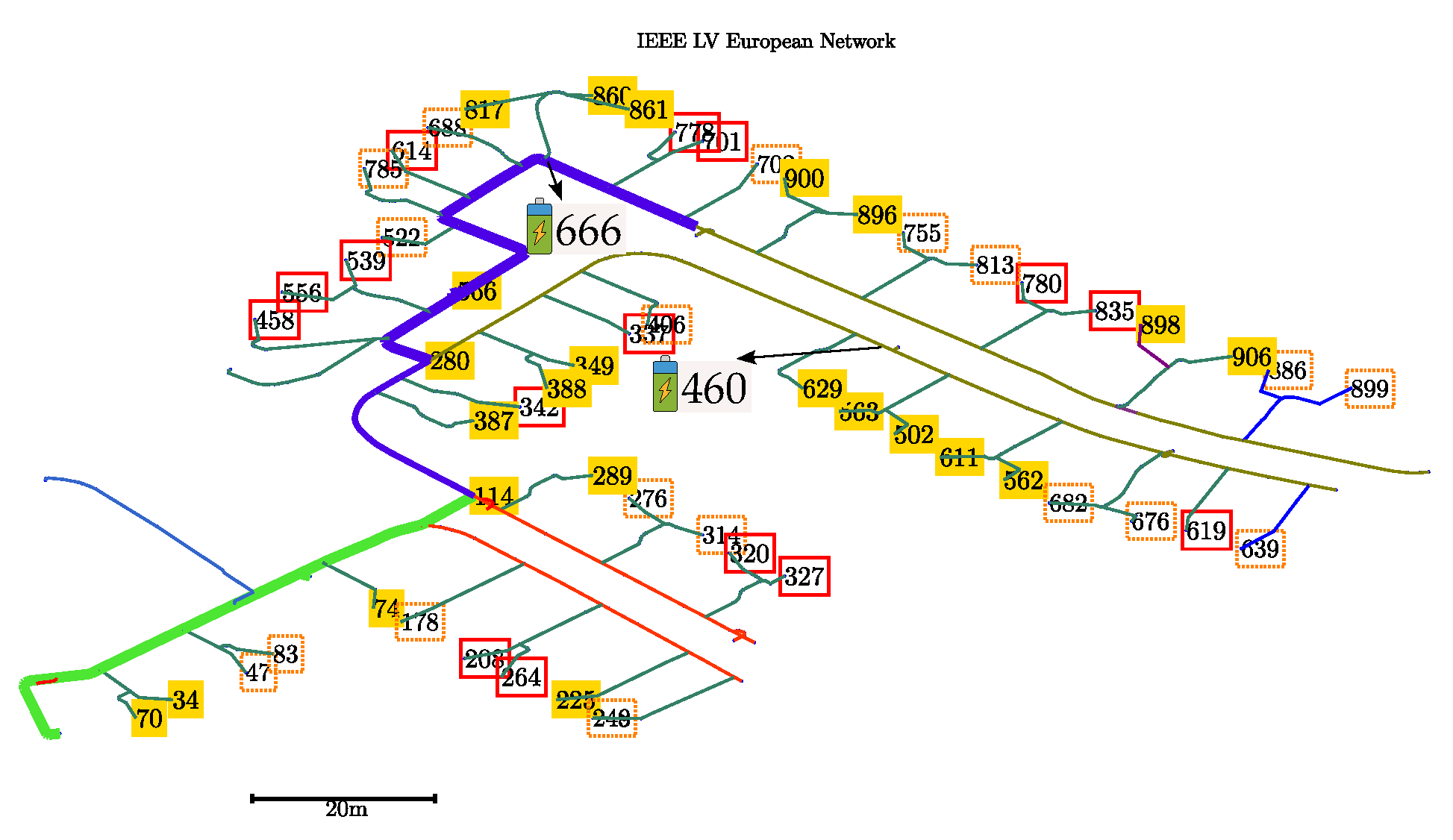
4. Case Study Synopsis

The validation of the proposed coordinated control of LV operation takes place for an IEEE LV benchmark network [52]. This LV grid—in Figure 4—presents the same technical characteristics with the benchmark with the difference that the MV/LV transformer 250 kVA, 20/0.4 kV, since only one feeder is regarded.

The MACOPF formulation is used to obtain the most suitable placement and sizing of the BESS for the examined grid. The results obtained, given the requirement of an energy BESS application—c-Rating 0.5—suggest the installation of a 90 kWh (round-trip efficiency considered to be 0.8) at node 460, and alternatively for distributed BESS solution one additional placed at node 666. The optimal sizing and placement problem performed co-optimizing the planning and operational services of the BESS (i.e., without the coordination with other assets or DER) for the 8-day dataset in 1-hour resolution (i.e., 384 time slots) for the mixed DER integration scenario 02; the same sizing and placement obtained are also used for all scenarios. In this particular planning stage, the BESS solution is used as the sole option to resolve the issues.

The definition of the examined scenarios is in

Table 3. Definition of examined scenarios.

	Case 01	Case 02	Case 03	Case 04
PV [nr of PV units]	30	30	0	20
EV [nr of EVs]	0	30	30	35

. The PV and EV integration refer as a percentage proportional to the number of units installed out of the total 55 consumers. Note that all DER are connected to the grid as single-phase units connected in the same phase as the respective end-user. Analytical information regarding the point of connections and the characteristics of DER can be found in [41]:

A data-set has been created for this study case to emulate and induct the results for yearly analysis. A data-pool of yearly load profiles (found in repository [53]) is statistically processed by using a k-means algorithm. Several sets of load profiles are aggregated and normalized to represent MV/LV substation’s profiles. This data are then properly clustered into seasons, weekends and weekdays. Regarding the clustering each centroid is considered as the component-wise median of that cluster, let it $c_i$. Each datapoint is accordingly clustered in Equation (27):

$$d(x,c)={\displaystyle \sum _{i=1}^{n_t}}|c_i-x_i|.$$

(27)

The representative data-set is thereafter composed of eight days, two per season (one representing weekdays and another one for weekends). Each of those is selected based on the centroid metric derived by k-means. The normalized aggregated at the substation level profiles are illustrated in Figure 5. To reproduce the load profiles, the inversed cumulative Gaussian distribution function (${\mathsf{\Phi }}^{-1}$) is set with maximum standard deviation $\sigma =0.08$ and median the value of the centroid at each datapoint. Therefore, each point of the load profile i at instant $\tau$ is calculated from Equation (28):

$$P_i\left(\tau \right)={\mathsf{\Phi }}^{-1}(c_i\left(\tau \right),\sigma )·P_{i,\mathrm{rated}}.$$

(28)

The Gaussian copula method is used to generate N temporal scenarios PV solar profiles, encapsulating the seasonal dependence as proposed in [54].

Prior to the presentation of the analytical case study, an assessment of incremental DER integration (EVs and PV) on operational grid constraints is conducted. In this part of the study, no controls are deployed; though any voltage issues, voltage unbalances, and any line congestions are recorded along the yearly data-set. For the following analysis, it should be noted that, for each scenario of DER integration, five days of the same season and type of day (i.e., weekday or weekend) are considered, and the resulting metrics (i.e., voltage magnitudes and unbalances) are averaged. The collected information is exported by sequential three-phase unbalanced power flow for averaged 30-minutes profiles. Obviously, the impact of DER in higher resolutions (e.g., order of minutes) may be more intensive (i.e., leading to more severe technical problems) particularly for phase unbalances and voltage issues. All the subsequent Figure 6, Figure 7 and Figure 8 represent the per season impact of integrating residential PV and EV. For all the incremental scenarios, random values of PV units (1.7, 2.7, 3.7 kW) and EVs (charging power outlet of 3.7 and 7.4 kW) are assigned accordingly.

The evolution of maximum and minimum voltage magnitudes met in the grid for integration of PV and EV appear in Figure 6a,b, respectively. One can notice the impact of inversed power flows due to microgeneration which lifts up both maximum and minimum voltage magnitudes. During summer periods, higher overvoltage are faced; meanwhile, higher overvoltage are more common during weekdays, since the loading conditions are lighter during sunny hours (see Figure 9a). In Figure 6a, the upper x-axis describes the PV integration correlated with the peak load as a percentage. For the considered load profiles, significant voltage increase (up to 1.07 p.u.) effects close to 50% of PV integration. In higher time resolution, voltage may experience, instantaneously, values higher than 1.1 p.u.; however, this study examines only a 30-minute average profile to determine maximum and minimum voltage limits as well to identify other technical bottlenecks on the safe operation of the grid. Regarding the EV integration, the minimum voltage up to 0.915 p.u. voltage appear with a number 40 EVs along the end-users. During weekends, due to lesser EV mileage, the demand for charging appears to be more limited compared to the weekdays. Furthermore, the simultaneity of charging at late evening hours (where daily peak load appears) leads to significant voltage drops.

The impact of connecting single phase DER on VUF is presented in Figure 7a,b. In all cases where no DER is installed, there are quite balanced conditions only up to 1.3%. The installation of microgeneration leads to an increase of VUF up to 2.1% during summer periods, which is justified due to lighter load conditions and higher PV generation. The connection of EVs increases a high amount of imbalance particularly in winter periods, where the loading conditions are intensive reaching up to 2.2%. The increasing integration of EV obviously leads to more severe phase unbalancing conditions. Being in accordance with IEC standards necessitates that VUF has to be less than 2% for 95% of the week [55]; hence, for this presented analysis—that is performed for 30-minute time slots—the VUF threshold is considered at 1.8%.

The connection of multiple PV units does not arise any line congestions up to 33% of their integration. Higher PV integration, though, results in excessive reversed power along the upstream grid, particularly overloading line 280–566 up to 0.98 p.u. of line currents. The line loading conditions are much more severe concerning the EV integration as illustrated in Figure 8b, where line congestions may reach up to 1.5 p.u. particularly in winter periods.

4.1. Results

This section demonstrates the techno-economical results for the examined cases of Table 3 performed with the proposed MACOPF scheme, among several modes of operation as defined in

Table 4. Definition of MACOPF setup along different modes of operation.

Operational Mode	Conventional Operation –No Smart Controls Applied– (m${}_0$)	DER Optimal Coordination (m${}_1$)	BESS Coordinated with DER (m${}_2$)	Distributed BESS Coordinated with DER (m${}_3$)	Coordination of OLTC with DER
OLTC	✕	✕	✕	✓	✓
BESS	✕	✕	✓	✕	✓
Smart Charging	✕	✓	✓	✓	✓
Vehicle to Grid	✕	✓	✓	✓	✓
$\mathsf{\mu }$G Active Power Curtailment	✓	✓	✓	✓	✓
$\mathsf{\mu }$G Reactive Power Dispatch	✕	✓	✓	✕	✕
Load Shedding	✓	✕	✕	✕	✕

. Note that the conventional mode of operation $m_0$, applies for controls with no particular intelligence. Such controls in this study are derived by executing sequential three-phase power flows to identify technical bottlenecks (i.e., line congestions or voltage issues). Based on an iterative process for every node with overvoltage, 5% of the produced energy is curtailed until the issue is resolved. Accordingly, EVs’ charging process is shed at the overloaded branches iteratively. The mode of operation $m_1$ refers to the sole coordination of all types of DER orchestrated by the MACOPF. It should be mentioned that, for this section, all EVs are considered available to provide grid support (i.e., through smart-charging), once they are parked at the house premises. Modes of operation $m_2$ and $m_3$ extend the aforementioned coordination with the utilization of one and two BESS—owned by the DSO—installed at nodes 460 and 666, accordingly. The last mode of operation stands for the coordinated operation of the OLTC with available DER for grid support.

The assigned costs for the utilization of each of the DER’s flexibility for this analysis are presented in

Table 5. Cost assumption for the case study.

	B	Cost (€/kWrh-kVArh)
Cost of Active Power Curtailment	$c_{apc}$	0.30
Cost Smart Charging	$c_{apc}$	0.15
Cost of V2G	$c_{V2G}$	0.35
Cost of Energy Not Supplied Lines	$c_{ENS}$	3

. Note that the active power curtailment is considered about three times larger than the price of selling the energy produced by residential $\mathsf{\mu }$G in Portugal. The main concern of the proposed scheme is to maximize the integration of microgeneration by exploiting other sources of flexibility, at the stage of the scheduling of operation. Concurrently, closer to the time of the delivery, APC may be used by typical droop control functions, ensuring safe grid operation. The cost of energy not supplied is set according to reports in [56]. The respective costs for the OLTC and BESS investment as well as the corresponding cost (summarized in Table 1 and Table 2) of their utilization are discussed in the previous sections together with their models. Concerning the OLTC investment, it is considered that the transformer’s remaining lifetime—and subsequently the OLTC investment lifetime—is 15 years.

The yearly operational costs for all modes of operation are illustrated in Figure 10a, while a breakdown of seasonal cost analysis appears in Figure 10b. One can notice that, in most scenarios, $m_0$ leads to higher operational costs than any coordinated operational scheme, apart from case 01 (i.e., where all modes are comparable). The increased connection of EVs in scenarios 02 and 04 leads to very high operational costs for $m_0$, due to the need for EV shedding in order to avoid branch congestions.

Commenting on case 01, where solely PV integration is regarded, one can notice that the cheapest operational modes of operation appear to be either the coordinated curtailment of PVs or the investment of OLTC. The curtailment of $\mu G$ should be followed by a compelling compensation fee as applied hereby; otherwise, such schemes should adopt fairness strategies. In this particular case, MACOPF on $m_1$ provides the optimal dispatch of active and reactive power leading to lower costs than in $m_0$. Indicatively, the curtailed energy for case 01 is in Figure 11a. Both cases $m_2-m_3$ lead to higher operational costs due to the topological distance of the BESS from the most problematic nodes (i.e., with overvoltage). Additionally, the BESS constraint for cyclic charging substantially increases the operational cost of BESS’s usage, since the absorbed energy—during sunny periods—will have to be consumed in other time slots, whether it is needed or not. For instance, BESS can be incorporated in MACOPF for extended energy management applications, where BESS are allowed to participate in the electricity market. In that case, grid operational costs for BESS usage would be more encouraging results, since the overall coordination of grid operation would follow the market price accordingly. More distributed BESS solutions may treat overvoltage by $\mu G$ more efficiently, depending on their spatial distribution along the grid. Nonetheless, the economical results between $m_3$–$m_4$ are closely equivalent since the tool decides the utilization of BESS placed at node 460 in both cases. Clearly, the OLTC presents very low annual operation costs in the vicinity of 350–700 € (i.e., depending on the remaining lifetime of the retrofitted transformer) for case 01, where solely PV are installed.

The installation of EVs in scenario 03 (no PVs) is followed by undervoltage and line congestions as analyzed previously. The yearly estimated operational costs due to the shedding of loads ($m_0$) reach up to 4.3 k€. The coordinated smart charging presents a much cheaper alternative of 1.6 k€. This price may slightly fluctuate considering the uncertainty of EV users that are willing to charge under this regime. It should be reminded that smart-charging hereby is strictly regarded when EVs are not in trip progress and refers to any deviation from the expected–dumb charging profile. An example from a typical winter day used in the simulations is in Figure 11b. The dumb charging profile for case 03 results in overloaded lines up to 1.09 p.u., a fact that is addressed with the coordinated smart charging in $m_1$. It can be observed that some charging profiles are shifted in slots with lesser loading conditions for the grid, which is the early morning hours as it appears in Figure 11b. In the same figure, it can be noticed that there is no V2G participation since the high EV availability concerned is capable of addressing the technical issues. In this scenario, the BESS coordinated operation presents much lower grid operational costs close to 750€ and about 700€ for $m_2$ and $m_3$, accordingly. The OLTC in this scenario—considering the 15 years lifetime of the transformer—presents annual costs close to 1.9 k€, due to the need for coordination with smart charging which pertains to 80% of this cost. Therefore, it is observed that the OLTC can only reduce the lines’ overload by lowering its taps; thus, the transformer’s secondary winding voltage is lifted up reducing the line currents analogously. This branch current reduction in this case of 5% (i.e., 1.09 p.u. reduced to 1.037 p.u.) on the most congested branch. From Figure 10b, it can be observed that the highest share of the operational costs comes from winter and autumn period, when the used data-set appears to have the peak demands.

Both scenarios 02 and 04 examine the integration of mixed DERs, considering extensive integration of PV and EV units. Case 02 is a PV rich scenario with the 30 single phase $\mathsf{\mu }$G, which corresponds to 49% of the peak demand of the grid. The last scenario 04 refers to a higher EV integration (35 EVs) and a 33% of the peak demand installed PV units. In both cases, the $m_0$ leads to high operational costs due to the need of EV shedding as well as an amount of 1.1 k€—case 02—for APC. Indicatively, Figure 12 presents analytically the control decisions derived from MACOPF for each mode of operation. It can be observed that along $m_1$, smart charging schedules shift some of the EVs during sunny period hours (i.e., 10.00–14.00), while some other EVs are further charged in the beginning of the day before the trip occurrences. The V2G mode of operation takes place not only to reduce line currents, but also to create available charging slots to be used during sunny periods with expected overvoltage. All EVs are constrained to keep their SoC at the end of the day equal to the one at the beginning of the simulation. Therefore, EVs that are parked at home all day present high availability, which is observed to be used in this way (i.e., charge during periods with high solar irradiance and discharge to avoid line congestions). Regarding OLTC operation, as illustrated in Figure 12d, it ends during the end of each day at tap –2, which is due to the loss minimization term. The OLTC acts in such way to increase the secondary winding voltage in order to avoid any voltage drops and minimize the active power losses as well. Obviously, the addition of some more EVs (case 04) results in a very abrupt increase of operational costs for $m_0$, a fact that is connected to the extensive line congestions that occur.

The proposed OLTC equipment is allowed to be set offline in different tap positions per phase to treat unbalances. The performed analysis considers 30-minute data resolution, a fact that may underestimate the real-time conditions regarding phase unbalances. Therefore, the OLTC may need further engagement with flexible DER to deal with phase unbalances; hence, higher operational costs may be foreseen in such a case.

4.1.1. Minimization of Active Power Losses

The annual active power losses without DER integration are estimated to be 1.5% to 2.5%, calculated through sequential power flow executions. From Figure 13, it can be observed that there is an increase in line losses due to the extensive DER integration, particularly when EVs are considered. The charging of the EVs does most likely occur during peak load period in the afternoon, increasing notably the loading along the distribution lines and to some extent the line losses (see Figure 13 reaching close to 6%).

In all cases and the subsequent modes of operation towards the resolution of technical bottlenecks (i.e., voltage magnitudes, voltage unbalances, and line congestions) line losses are also reduced compared to the scenario where no controls are applied. Particularly, modes $m_1$–$m_4$ based on the proposed MACOPF control framework do further reduce the line losses due to the involved objective term. The coordinated operation of the OLTC with DER appears to perform the most efficient measure in the direction of losses minimization. Additionally, experimenting (i.e., by assigning higher values to $w_2$) with the weighted terms among the objective terms in modes $m_1$–$m_3$ does not impact significantly the control decisions and the losses. The latter can be justified due to the fact that further minimization of active power losses, substantially, precedes more engagement of DER flexibility. Nonetheless, involving more flexibility in the scheduling of operation for the the losses minimization cannot be justified economically.

The exploitation of the OLTC brings greater benefit to the objective, particularly for the minimization of active power losses, since the low cost per tap operation allows the optimizer to derive taps-down, lifting the primary side to higher voltage.On the other hand, the combination of BESS or smart charging cannot justify their excessive usage towards further minimization of losses at the same order of reduction compared to the OLTC.

4.1.2. Sensitivity Analysis on BESS and Smart-Charging Coordination

A sensitivity analysis is presented hereby to observe the evolution of the estimated DSO annual operational costs for different prices of smart charging and different LCOE for the BESS. This section provides a comprehensive comparative analysis not only in the reflection of the pricing of EV flexibility—i.e., EV available for smart charging—and the BESS, into the DSO equivalent annual cost of operation, but also signifies the importance of enabling EV smart charging towards the reduction of operational costs. Furthermore, one scenario concerns the V2G mode of operation in the sensitivity analysis. Along the evolution of BESS and EV pricing and their availability (i.e., spatio-temporal), the resulting coordination is recorded through the proposed control scheme.

In each case, the range of BESS prices lies within [200–380] €/kWh (i.e., corresponding LCOE [0.05, 0.0925] €/kWh) according to the study in [26], for base year 2025. For the purpose of this study, scenario 02 is considered regarding the integration of DER. The cost of utilizing EV flexibility is considered in the range [0.05, 0.25] € for each kWh of shifted charging slot.

On the data-points in Figure 14, the coordination of EV and BESS is displayed as a share of the annual DSO operation costs. As BESS price increases, the EVs’ flexibility is further used following a quasi-linear dependence and vice versa. Note that, particularly in Figure 14a, where only 20% of the connected EVs are considered as flexible, even when BESS cost is higher than the EV flexibility, the limited EV availability forces the resolution of technical bottlenecks mainly with the use of BESS. On the other hand, one can notice that, in Figure 14b, the higher availability of EVs—60%–(which implies better spatio-temporal distribution) leads to reduced DSO costs in most cases (see data-points in Figure 14b). The fact that EVs are distributed along the grid is foreseen to be very efficient to address any technical bottlenecks arising from PV and EV integration. The latter can be further observed when all EVs are considered as flexible in Figure 14c, where the effect on the cost reduction is more intensive since the plane follows—an affine—curvature. The last sensitivity analysis considers V2G in constant pricing at 0.35 €/kWh, combined with 100% EV availability for smart charging. The fact that V2G is considered in the framework essentially allows the utilization of EVs that do not proceed with a trip (i.e., and then they have to get charged, since they are constrained to recharge in the simulation day at least the energy used). The effective coordination of the BESS, EV smart charging, and V2G leads to notably lesser grid operational costs compared to other cases. Note that the maximum cost observed when BESS and EV are assigned with the highest price values is 1.6 k€, when the resulting maximum cost in the other planes reaches close to 2.5 k€.

5. Conclusions

This work presents a control framework that derives the coordinated management for multiple DSO assets and DER, in a way to ensure safe grid operation pertaining admissible voltage magnitudes, phase balancing, and avoiding line congestions. The overall scheme is formulated as a nonlinear multi-objective program resolved with a primal-dual interior point algorithm. A three-stage technique is proposed to incorporate the OLTC in the decision-making process. The control framework is advanced and adapted to propose efficient decisions for the placement and sizing of BESS.

The study shows that OLTC appears to be the most efficient option to treat overvoltage when high PV integration is encountered, considering loss minimization. Nonetheless, phase unbalances may occur that could be treated by coordinating with other DER, or the installation of BESS. It was concluded that, for long-term phase imbalances, the OLTC can be also setup in offline mode to proper tap positions per winding—hence reducing the unbalances and the need of coordination with other assets or DER. The extensive integration of EVs (more than 20 EVs in the examined case) cannot be accommodated only by the optimal operation of the OLTC. In the presented study the OLTC is capable of reducing the overloading to 25–32% of the most congested branches; however, coordination with EVs is deemed necessary to respect all technical constraints. Depending on the selected OLTC technology and whether the transformer can be retrofitted—as examined in this study—the OLTC is foreseen to be most efficient to address reversed power flows effects and the subsequent overvoltage. On the other hand, BESS’s solution is very dependent on the expected costs along the evolution in the next decade. Considering a moderate BESS cost (i.e., regarding the expected adoption of BESS in the market) presents comparable results—or better results in some cases—with OLTC. In mixed DER scenarios (i.e., PV and EV), BESS coordinated with DER outperforms the compared modes of operation, presenting the lowest DSO annual equivalent operational costs.

A sensitivity analysis demonstrated the DSO’s annual costs of operation considering different costs for BESS and EV flexibility utilization. The main outcome of this sensitivity study shows the importance, due to their spatio-temporal distribution, of the active participation of DER (i.e., mainly for EVs with V2G hereby) in the grid operation and the significant reflection on cost reduction.

References

1. Bruno, S.; La Scala, M. Unbalanced Three-Phase Optimal Power Flow for the Optimization of MV and LV Distribution Grids. In From Smart Grids to Smart Cities: New Challenges in Optimizing Energy Grids; John Wiley & Sons: Hoboken, NJ, USA, 2017; pp. 1–42. [Google Scholar]
2. Hatziargyriou, N.; Vlachokyriakou, O.; Van Cutsem, T.; Milanovic, J.; Pourbeik, P.; Vournas, C.; Hong, M.; Ramos, R.; Boemer, J.; Aristidou, P. Task Force on Contribution to Bulk System Control and Stability by Distributed Energy Resources Connected at Distribution Network; Rep. PES-TR22; IEEE PES: Piscataway, NJ, USA, 2017. [Google Scholar]
3. Razavi, S.E.; Rahimi, E.; Javadi, M.S.; Nezhad, A.E.; Lotfi, M.; Shafie-khah, M.; Catalão, J.P.S. Impact of distributed generation on protection and voltage regulation of distribution systems: A review. Renew. Sustain. Energy Rev. 2019, 105, 157–167. [Google Scholar] [CrossRef]
4. Bruno, S.; Lamonaca, S.; Rotondo, G.; Stecchi, U.; La Scala, M. Unbalanced three-phase optimal power flow for smart grids. IEEE Trans. Ind. Electron. 2011, 58, 4504–4513. [Google Scholar] [CrossRef]
5. Lotfi, M.; Monteiro, C.; Shafie-khah, M.; Catalão, J.P.S. Evolution of Demand Response: A Historical Analysis of Legislation and Research Trends. In Proceedings of the 2018 Twentieth International Middle East Power Systems Conference (MEPCON), Cairo, Egypt, 18–20 December 2018; pp. 968–973. [Google Scholar] [CrossRef]
6. Rodrigues, J.; Moreira, C.; Lopes, J.A. Smart Transformers as Active Interfaces Enabling the Provision of Power-Frequency Regulation Services from Distributed Resources in Hybrid AC/DC Grids. Appl. Sci. 2020, 10, 1434. [Google Scholar] [CrossRef] [Green Version]
7. Karagiannopoulos, S.; Aristidou, P.; Hug, G. A Centralised Control Method for Tackling Unbalances in Active Distribution Grids. In Proceedings of the IEEE 2018 Power Systems Computation Conference (PSCC), Dublin, Ireland, 11–15 June 2018. [Google Scholar]
8. Borghetti, A.; Bosetti, M.; Grillo, S.; Massucco, S.; Nucci, C.A.; Paolone, M.; Silvestro, F. Short-Term Scheduling and Control of Active Distribution Systems With High Penetration of Renewable Resources. IEEE Syst. J. 2010, 4, 313–322. [Google Scholar] [CrossRef]
9. Et-Taoussi, M.; Ouadi, H.; Chakir, H.E. Hybrid optimal management of active and reactive power flow in a smart microgrid with photovoltaic generation. Microsyst. Technol. 2019. [Google Scholar] [CrossRef]
10. Olivier, F.; Aristidou, P.; Ernst, D.; Cutsem, T.V. Active Management of Low-Voltage Networks for Mitigating Overvoltage Due to Photovoltaic Units. IEEE Trans. Smart Grid 2016, 7, 926–936. [Google Scholar] [CrossRef] [Green Version]
11. Karagiannopoulos, S.; Aristidou, P.; Hug, G. Data-driven Local Control Design for Active Distribution Grids using offline Optimal Power Flow and Machine Learning Techniques. IEEE Trans. Smart Grid 2019. [Google Scholar] [CrossRef]
12. Lilla, S.; Orozco, C.; Borghetti, A.; Napolitano, F.; Tossani, F. Day-ahead scheduling of a local energy community: An alternating direction method of multipliers approach. IEEE Trans. Power Syst. 2019. [Google Scholar] [CrossRef]
13. Karambelkar, S.; Mackay, L.; Chakraborty, S.; Ramirez-Elizondo, L.; Bauer, P. Distributed Optimal Power Flow for DC Distribution Grids. In Proceedings of the 2018 IEEE Power & Energy Society General Meeting (PESGM), Portland, OR, USA, 5–10 August 2018; pp. 1–5. [Google Scholar] [CrossRef]
14. Karfopoulos, E.L.; Panourgias, K.A.; Hatziargyriou, N.D. Distributed Coordination of Electric Vehicles providing V2G Regulation Services. IEEE Trans. Power Syst. 2016, 31, 2834–2846. [Google Scholar] [CrossRef]
15. Efkarpidis, N.; De Rybel, T.; Driesen, J. Optimal placement and sizing of active in-line voltage regulators in flemish LV distribution grids. IEEE Trans. Ind. Appl. 2016, 52, 4577–4584. [Google Scholar] [CrossRef]
16. Shahnia, F.; Majumder, R.; Ghosh, A.; Ledwich, G.; Zare, F. Voltage imbalance analysis in residential low voltage distribution networks with rooftop PVs. Electr. Power Syst. Res. 2011, 81, 1805–1814. [Google Scholar] [CrossRef]
17. Degroote, L.; Renders, B.; Meersman, B.; Vandevelde, L. Neutral-point shifting and voltage unbalance due to single-phase DG units in low voltage distribution networks. In Proceedings of the 2009 IEEE Bucharest PowerTech, Bucharest, Romania, 28 June–2 July 2009; pp. 1–8. [Google Scholar] [CrossRef]
18. Efkarpidis, N.; De Rybel, T.; Driesen, J. Technical assessment of centralized and localized voltage control strategies in low voltage networks. Sustain. Energy Grids Netw. 2016, 8, 85–97. [Google Scholar] [CrossRef]
19. Demirok, E.; González, P.C.; Frederiksen, K.H.B.; Sera, D.; Rodriguez, P.; Teodorescu, R. Local Reactive Power Control Methods for Overvoltage Prevention of Distributed Solar Inverters in Low-Voltage Grids. IEEE J. Photovoltaics 2011, 1, 174–182. [Google Scholar] [CrossRef]
20. Cagnano, A.; De Tuglie, E.; Liserre, M.; Mastromauro, R.A. Online optimal reactive power control strategy of PV inverters. IEEE Trans. Ind. Electron. 2011, 58, 4549–4558. [Google Scholar] [CrossRef]
21. Heleno, M.; Rua, D.; Gouveia, C.; Madureira, A.; Matos, M.A.; Lopes, J.P.; Silva, N.; Salustio, S. Optimizing PV self-consumption through electric water heater modeling and scheduling. In Proceedings of the 2015 IEEE Eindhoven PowerTech, Eindhoven, The Netherlands, 29 June–2 July 2015; pp. 1–6. [Google Scholar] [CrossRef]
22. Stetz, T.; Marten, F.; Braun, M. Improved low voltage grid-integration of photovoltaic systems in Germany. IEEE Trans. Sustain. Energy 2012, 4, 534–542. [Google Scholar] [CrossRef]
23. Su, X.; Masoum, M.A.S.; Wolfs, P.J. Multi-Objective Hierarchical Control of Unbalanced Distribution Networks to Accommodate More Renewable Connections in the Smart Grid Era. IEEE Trans. Power Syst. 2016, 31, 3924–3936. [Google Scholar] [CrossRef]
24. Samadi, A.; Shayesteh, E.; Eriksson, R.; Rawn, B.; Söder, L. Multi-objective coordinated droop-based voltage regulation in distribution grids with PV systems. Renew. Energy 2014, 71, 315–323. [Google Scholar] [CrossRef]
25. Petrou, K.; Procopiou, A.; Ochoa, L.F.; Langstaff, T.; Theunissen, J. Residential Battery Controller For Solar PV Impact Mitigation: A Practical and Customer-friendly Approach; AIM: Madrid, Spain, 2019. [Google Scholar]
26. Tsiropoulos, I.; Tarvydas, D.; Lebedeva, N. Li-ion Batteries for Mobility and Stationary Storage Applications Scenarios for Costs and Market Growth; Publications Office of the European Union: Luxembourg, 2018. [Google Scholar]
27. Aghaei, J.; Bozorgavari, S.A.; Pirouzi, S.; Farahmand, H.; Korpås, M. Flexibility Planning of Distributed Battery Energy Storage Systems in Smart Distribution Networks. Iran. J. Sci. Technol. Trans. Electr. Eng. 2019. [Google Scholar] [CrossRef]
28. Miranda, I.; Leite, H.; Silva, N. Coordination of multifunctional distributed energy storage systems in distribution networks. IET Gener. Transm. Distrib. 2016, 10, 726–735. [Google Scholar] [CrossRef]
29. Union, E. Directive 2009/72/ec of the european parliament and of the council of 13 july 2009 concerning common rules for the internal market in electricity and repealing directive 2003/54/ec. Off. J. Eur. Union 2009, 211, 55–93. [Google Scholar]
30. Efkarpidis, N.; De Rybel, T.; Driesen, J. Optimization control scheme utilizing small-scale distributed generators and OLTC distribution transformers. Sustain. Energy Grids Netw. 2016, 8, 74–84. [Google Scholar] [CrossRef]
31. Lopes, J.A.P.; Soares, F.J.; Almeida, P.M.R. Integration of electric vehicles in the electric power system. Proc. IEEE 2010, 99, 168–183. [Google Scholar] [CrossRef] [Green Version]
32. Sharma, I.; Cañizares, C.; Bhattacharya, K. Smart Charging of PEVs Penetrating Into Residential Distribution Systems. IEEE Trans. Smart Grid 2014, 5, 1196–1209. [Google Scholar] [CrossRef]
33. Richardson, P.; Flynn, D.; Keane, A. Optimal Charging of Electric Vehicles in Low-Voltage Distribution Systems. IEEE Trans. Power Syst. 2012, 27, 268–279. [Google Scholar] [CrossRef] [Green Version]
34. García-Villalobos, J.; Zamora, I.; Knezović, K.; Marinelli, M. Multi-objective optimization control of plug-in electric vehicles in low voltage distribution networks. Appl. Energy 2016, 180, 155–168. [Google Scholar] [CrossRef] [Green Version]
35. Connell, A.O.; Flynn, D.; Keane, A. Rolling Multi-Period Optimization to Control Electric Vehicle Charging in Distribution Networks. IEEE Trans. Power Syst. 2014, 29, 340–348. [Google Scholar] [CrossRef]
36. Jiricka, J.; Kaspirek, M.; Kolar, L.; Zahradka, M. Smart substation MV/LV. CIRED Open Access Proc. J. 2017, 2017, 1482–1486. [Google Scholar] [CrossRef]
37. Liu, X.; Aichhorn, A.; Liu, L.; Li, H. Coordinated Control of Distributed Energy Storage System with Tap Changer Transformers for Voltage Rise Mitigation Under High Photovoltaic Penetration. IEEE Trans. Smart Grid 2012, 3, 897–906. [Google Scholar] [CrossRef]
38. Maniatopoulos, M.; Lagos, D.; Kotsampopoulos, P.; Hatziargyriou, N. Combined control and power hardware in-the-loop simulation for testing smart grid control algorithms. IET Gener. Transm. Distrib. 2017, 11, 3009–3018. [Google Scholar] [CrossRef]
39. Kulmala, A.; Repo, S.; Järventausta, P. Coordinated Voltage Control in Distribution Networks Including Several Distributed Energy Resources. IEEE Trans. Smart Grid 2014, 5, 2010–2020. [Google Scholar] [CrossRef]
40. Fortenbacher, P.; Zellner, M.; Andersson, G. Optimal sizing and placement of distributed storage in low voltage networks. In Proceedings of the 2016 Power Systems Computation Conference (PSCC), Genoa, Italy, 20–24 June 2016; pp. 1–7. [Google Scholar] [CrossRef] [Green Version]
41. Kotsalos, K.; Miranda, I.; Silva, N.; Leite, H. A Horizon Optimization Control Framework for the Coordinated Operation of Multiple Distributed Energy Resources in Low Voltage Distribution Networks. Energies 2019, 12, 1182. [Google Scholar] [CrossRef] [Green Version]
42. Kotsalos, K.; Domingues-Garcia, J.L.; Hatziargyriou, N.; Miranda, I.; Leite, H.; Silva, N. Coordinated Management of Distributed Energy Resources in Smart Microgrids. In Proceedings of the IECON 2019-45th Annual Conference of the IEEE Industrial Electronics Society, Lisbon, Portugal, 14–17 October 2019. [Google Scholar]
43. Ciric, R.M.; Feltrin, A.P.; Ochoa, L.F. Power flow in four-wire distribution networks-general approach. IEEE Trans. Power Syst. 2003, 18, 1283–1290. [Google Scholar] [CrossRef] [Green Version]
44. Zimmerman, R.D.; Murillo-Sánchez, C.E. MATPOWER 6.0 User’S Manual; Power Systems Engineering Research Center: Arizona, AZ, USA, 2016; Volume 9. [Google Scholar]
45. Nocedal, J.; Wright, S.J. Numerical Optimization, 2nd ed.; Springer Science & Business Media: Cham, Switzerland, 2006; pp. 497–528. [Google Scholar]
46. Wang, Y.J. Analysis of effects of three-phase voltage unbalance on induction motors with emphasis on the angle of the complex voltage unbalance factor. IEEE Trans. Energy Convers. 2001, 16, 270–275. [Google Scholar] [CrossRef]
47. Jen-Hao, T. A direct approach for distribution system load flow solutions. IEEE Trans. Power Deliv. 2003, 18, 882–887. [Google Scholar] [CrossRef]
48. Zhu, J. Optimization of Power System Operation; John Wiley & Sons, Inc.: Hoboken, NJ, USA, 2015; pp. 1–12. [Google Scholar] [CrossRef]
49. Burer, S.; Letchford, A.N. Non-convex mixed-integer nonlinear programming: A survey. Surv. Oper. Res. Manag. Sci. 2012, 17, 97–106. [Google Scholar] [CrossRef] [Green Version]
50. Timbus, A.; Larsson, M.; Yuen, C. Active management of distributed energy resources using standardized communications and modern information technologies. IEEE Trans. Ind. Electron. 2009, 56, 4029–4037. [Google Scholar] [CrossRef]
51. Le Digabel, S. Algorithm 909: NOMAD: Nonlinear optimization with the MADS algorithm. ACM Trans. Math. Softw. (TOMS) 2011, 37, 44. [Google Scholar] [CrossRef]
52. Espinosa, A.N. Dissemination Document “Low Voltage Networks Models and Low Carbon Technology Profiles”; The University of Manchester: Manchester, UK, 2015. [Google Scholar]
53. Pedersen, R.; Sloth, C.; Andresen, G.B.; Wisniewski, R. DiSC: A simulation framework for distribution system voltage control. In Proceedings of the 2015 European Control Conference (ECC), Linz, Austria, 15–17 July 2015; pp. 1056–1063. [Google Scholar]
54. Pinto, R.; Bessa, R.J.; Matos, M.A. Multi-period flexibility forecast for low voltage prosumers. Energy 2017, 141, 2251–2263. [Google Scholar] [CrossRef] [Green Version]
55. Masetti, C. Revision of European Standard EN 50160 on power quality: Reasons and solutions. In Proceedings of the 14th International Conference on Harmonics and Quality of Power (ICHQP 2010), Bergamo, Italy, 26–29 September 2010; pp. 1–7. [Google Scholar]
56. dos Serviços Energéticos, E.E.R. Parâmetros de Regulação para o Período 2015–2017; Entidade Reguladora Dos ServiçOs EnergéTicos: Lisboa, Portugal, 2014. [Google Scholar]
57. Cheng, C.S.; Shirmohammadi, D. A three-phase power flow method for real-time distribution system analysis. IEEE Trans. Power Syst. 1995, 10, 671–679. [Google Scholar]
58. Bazrafshan, M.; Gatsis, N. Comprehensive Modeling of Three-Phase Distribution Systems via the Bus Admittance Matrix. IEEE Trans. Power Syst. 2018, 33, 2015–2029. [Google Scholar] [CrossRef] [Green Version]
Figure 1. Representation of OLTC connected with the upstream grid.
Sustainability 12 03332 g001
Figure 2. Proposed optimization scheme for the OLTC.
Sustainability 12 03332 g002
Figure 3. (a) cost function assignment for smart charging; (b) example of smart charging operation.
Sustainability 12 03332 g003
Figure 4. The IEEE European LV benchmark network. Fifty-five consumers are connected to this case network.
Sustainability 12 03332 g004
Figure 5. Classification of aggregated normalized loads (at the secondary substation level). The red line represents the centroid of the k-means.
Sustainability 12 03332 g005
Figure 6. Minimum and maximum voltage according to the seasonal data over: (a) incremental PV integration; and (b) incremental EV integration seasonal (e.g., summer profiles) and regional data.
Sustainability 12 03332 g006
Figure 7. The range of maximum voltage unbalances according to the seasonal data over: (a) incremental PV integration; and (b) incremental EV integration seasonal (e.g., summer profiles) and regional data.
Sustainability 12 03332 g007
Figure 8. The total number of congested phases on the seasonal data over: (a) incremental PV integration and (b) incremental EV integration seasonal (e.g., summer profiles) and regional data.
Sustainability 12 03332 g008
Figure 9. (a) Seasonal load demand at secondary substation and (b) trips in progress during a week.
Sustainability 12 03332 g009
Figure 10. Annual DSO operational costs for all modes of operation m 0 m 4 : (a) over the examined scenarios; and (b) seasonal breakdown annual costs.
Sustainability 12 03332 g010
Figure 11. Control actions derived for case 01 ( m 1 ) and case 03 m 3 : (a) active power curtailments and reactive power dispatch to regulate voltage; and (b) smart EV charging schedules to avoid voltage drops and lines overloading.
Sustainability 12 03332 g011
Figure 12. Control actions derived from MACOPF for case 02 along the examined modes of operation: (a) m 1 ; (b) m 2 ; (c) m 3 ; and (d) m 4 .
Sustainability 12 03332 g012
Figure 13. Annual active power losses for each scenario and each mode of operation.
Sustainability 12 03332 g013
Figure 14. Annual operational costs for different shares of EV willing to participate in smart charging: (a) 20% flexible EVs; (b) 60% flexible EVs; (c)100% flexible EVs; and (d) 100% flexible EVs and V2G mode of operation are also available.
Sustainability 12 03332 g014