A Topological Analysis of Trade Distance: Evidence from the Gravity Model and Complex Flow Networks


1
School of Systems Science, Beijing Normal University, Beijing 100875, China
2
Business School, Beijing Normal University, Beijing 100875, China
3
Department of Astronomy, Beijing Normal University, Beijing 100875, China
*
Author to whom correspondence should be addressed.
Sustainability 2020, 12(9), 3511; https://0-doi-org.brum.beds.ac.uk/10.3390/su12093511
Submission received: 3 March 2020
/
Revised: 14 April 2020
/
Accepted: 14 April 2020
/
Published: 25 April 2020
(This article belongs to the Section Economic and Business Aspects of Sustainability)
Abstract
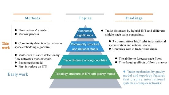
:As a classical trade model, the gravity model plays an important role in the trade policy-making process. However, the effect of physical distance fails to capture the effects of globalization and even ignores the multilateral resistance of trade. Here, we propose a general model describing the effective distance of trade according to multilateral trade paths information and the structure of the trade flow network. Quantifying effective trade distance aims to identify the hidden resistance information from trade networks data, and then describe trade barriers. The results show that flow distance, hybrid by multi-path constraint, and international trade network contribute to the forecasting of trade flows. Meanwhile, we also analyze the role of flow distance in international trade from two perspectives of network science and econometric model. At the econometric model level, flow distance can collapse to the predicting results of geographic distance in the proper time lagging variable, which can also reflect that flow distance contains geographical factors. At the international trade network level, community structure detection by flow distances and flow space embedding instructed that the formation of international trade networks is the tradeoff of international specialization in the trade value chain and geographical aggregation. The methodology and results can be generalized to the study of all kinds of product trade systems.
1. Introduction
International trade is one of the most important economic activities among countries, and its effect on one country’s economic growth is self-evident. Forecasting international trade flows is critical to assessing economic growth. International trade data, as a non-monetary tool to measure the complexity of national economies, have greatly enriched the assessment and prediction of the growth performance of individual economies [1,2,3,4,5,6]. For example, Hausmann, the renowned economist, proposed the concept of economic complexity in the dimension of international trade to quantitatively evaluate a country’s future economic growth potential: the gap of countries’ economic growth depends on the diversity of their exports, which also causes that the national development has the path-dependence property. This makes it possible to rely on historical data to predict short-term economic growth, and there is a correlation among investments, performance, and economic growth [7,8].
For the long term, the gravity model describes the pattern of total bilateral trade flows [9,10]: trade flows are proportional to the size of a country’s economy and inversely proportional to the distance between them, because of the cost of transportation. Although the role of economic size has been well understood in various theoretical contexts, the interpretation of the role of distance has been controversial [11], especially with some counter-intuitive empirical results. For example, Head and Mayer reviewed 161 published papers using 1835 estimates of the midrange coefficient for gravity-type regression [12]. The results from the different samples were surprisingly stable, which reflects the issue of the “missing globalization puzzle” in the trade fields: physical distance cannot capture the effects of globalization and remains constant over time in the gravity model. Physical distance can represent trade distance and costs to some extent; however, it fails to reflect the multi-polarization and multi-resistance effect of international trade brought about by globalization [13].
Over the recent decades of globalization, the world has interacted more closely than ever before. On the one hand, population, resources, and sustainable development affect the industrial pattern of countries, thereby it will lead to the complexity of international trade [14]. Because the trading system is complex, time-varying, and nonlinear, it is necessary to use a system approach, such as using complex network model, to empirically model the interactions. On the other hand, since international trade is the result of the constraints of trade barriers and economic and political games, trade barriers and trade networks coevolve. It provides an intrinsic basis for characterizing trade barriers by the historical data of trade, i.e., the hidden resistance information can be filtered from the topological structure of trade networks. The measure of trade resistances or trade barriers is defined as the effective distance of trade systems in this paper. By doing this, we compute the “effective trade distance” from the perspective of multilateral resistance and network effect. Then, a rolling-windows approach is used to consider the potential time-varying relationship in the distance measure, thereby helping to forecast the complexity of the economic system.
Using the complex network model to study international trade is to capture the backbone of trade systems by abstracting countries and their trade relations into nodes and edges. The purpose of this paper is to overcome the “missing globalization puzzle” to establish a measure of “effective trade distance” with the time-varying and potential multi-resistance characteristics.
2. Literature Review
The role of trade costs in the international economic system has been extensively discussed and widely used in many fields [15,16]. Especially, physical distance is regarded as the most common proxy for international trade costs [12,17]. In the earliest contribution of this issue, the authors modified the gravity model by adding different explanatory variables [18,19], e.g. bilateral distance effects measured by the fixed costs. For example, Manova and Zhang fixed costs that are increasing with distance [20] or firm search costs for buyers [21]. Yi also argued that fragmentation can explain the nonlinear effects of trade costs on trade [22].
However, the drawback is that the estimated results fail to capture the effect of globalization, which is defined as the “missing globalization puzzle”: it remains constant over time. Many economic studies have attempted to resolve this issue with mixed success [23,24,25,26]. This approach requires the addition of more explanatory items when more factors are considered, which may lead to gravity models extremely bloated. Especially, some variables have strong economic significance, but are highly correlated and pose multicollinearity problems.
Additionally, the effects of globalization should also be reflected in increasing estimates of the effects of contiguous borders, which reflect the effects of globalization that may travel through the middle trade, i.e., global value chains may first be established regionally, thereby reinforcing trade with neighboring countries in gravity estimations. For example, Marek Maciejewski illustrated that attractiveness can be expressed as the common border of many factors [27]. Moreover, intermediate merchandise trade has a different impact on the final products in the aspect of product and factor prices. Research shows that intermediate merchandise trade can promote exports, increase R&D investment, and positively affect innovation [28,29], thereby improving productivity and promoting the quality of export products [30]. Quantitative analysis of the impact of the real distance between the import and export of commodities on trade is relatively rare, especially the export to domestic sales, intermediate products trade, etc. because measuring these trade distances is complicated. Quantifying the distance cost of intermediate trade is very complicated, we thus need to find new research paradigms to address this problem.
The elasticity of distance may change in both directions as the market size changes [12], and an empirical model of scale effects can be explained by the relevant export-dynamic network (International Trade Network, ITN). The significant difference of ITN from the gravity model is that many dimensions of trade information have been embedded virtually in ITN, rather than infinitely added explanatory variables because ITN is formed by the interaction of national behaviors and multiple factors that have already covered politics, culture, and other information. Another stream of literature has examined how complex network measures affect key international trade, which mainly focuses on multi-scale models of multilateral trade based on a network topology from the real trade data.
In that case, how can we define the “effective trade distance”? There are already different distance measures proposed based on network theory [31,32]. Despite the success of these distances for analyzing practical issues, they suffer from defects in studying trade problems. The most obvious shortcomings is that network distance, such as hyperbolic distance and shortest path distance, seldom consider the trade flow information. Additionally, although Brockman’s effective distance subsumes the information of the topology and the flux on edges, this method only calculates the distance of the most possible (maximum likelihood) paths between nodes but does not count all paths. Conversely, with the rise of the global industrial chain, trade flows can be recognized as part of a longer value chain. This information is encoded into all the paths along with the trade flow network. It is not enough if we only consider the most possible path, and economic behavior is often not driven by probability. On the contrary, with the rise of global industrial chains, trade flows can be considered as part of a longer value chain, and this information is encoded into all paths of the trade flow network, rather than the most possible path. Therefore, the definition of effective distance should hybrid trade networks and full path constraints.
Following the existing literature, which provides a good foundation for setting up the empirical model, this paper aims to make the following contributions to construct the “effective trade distance”. It can identify the real trade distance—flow distance—which emphasizes the networks of trade relations under multilateral interactions and the structure of the global production value chain.
3. Methods
3.1. Data
All of the data used in this article are from open source databases that can be downloaded from corresponding websites. The data for international trade come from the United Nations commodity trade statistics database. The data we use are 97 categories of product data with 2-bite customs codes from 1996 to 2016, covering the information on trade relations and trade volume among countries. The geographic distance data come from the CEPII database (http://www.cepii.fr/). The geographic distance between national capitals is used as the distance variable of the gravity model. GDP, energy net export, s and domestic energy use were obtained from the world bank from 1996 to 2016 (https://data.worldbank.org.cn/).
3.2. Construction of International Trade Flow Networks
As a supplementary and typical example, we build the international trade flow network and make empirical analyses using the latest achievements of complex network theory. We employ international trade data that are available from the United Nations commodity trade statistics database, which contains data on the value of trades between countries and their trading partners. The dataset provides both import and export trade data. Here, the ITN can be described as a directed weighted network, where nodes and directed links represent all of the countries and their imports and export relationships, respectively. From the perspective of network science, a country can be abstracted into a node and export or outport trade relationships can be abstracted into a link in the international trade networks.
The framework of complex networks study, enabling us to understand international trade as a whole, offers a new perspective of connection to explore the issue of trade systems with more information, such as the core/periphery structure [33,34], the role of WTO [35], the robustness of trade systems (stability of the international trade system) [34,36], problems of critical propagation in ITN [37,38], and so on. Additionally, ITN can be regarded as a space where international trade is formed by the interaction of national behaviors and multiple factors that have already covered politics, culture, and other information. This understanding may help us to reconsider the distance effect on the gravity model, capturing the features of effective trade distance, including time-varying, multilateral resistance, and network effects.
However, the most obvious shortcomings is that network distance, such as hyperbolic distance and shortest path distance, seldom consider the intrinsic mechanism of trade flow information and trade distance. The international trade system is constructed by exchanging the flow of commodities [39] and restricted by the natural resources, technological level, and production capacity of each country. From the perspective of trade flow, the international trade system is an open system that describes how the energy, substance, products, and money exchange between resources of the external environment and trade relations of an inter-system [40]. Thus, we use an open system approach to characterize international trade, known as the International Trade Flow Network (ITFN) [41,42,43].
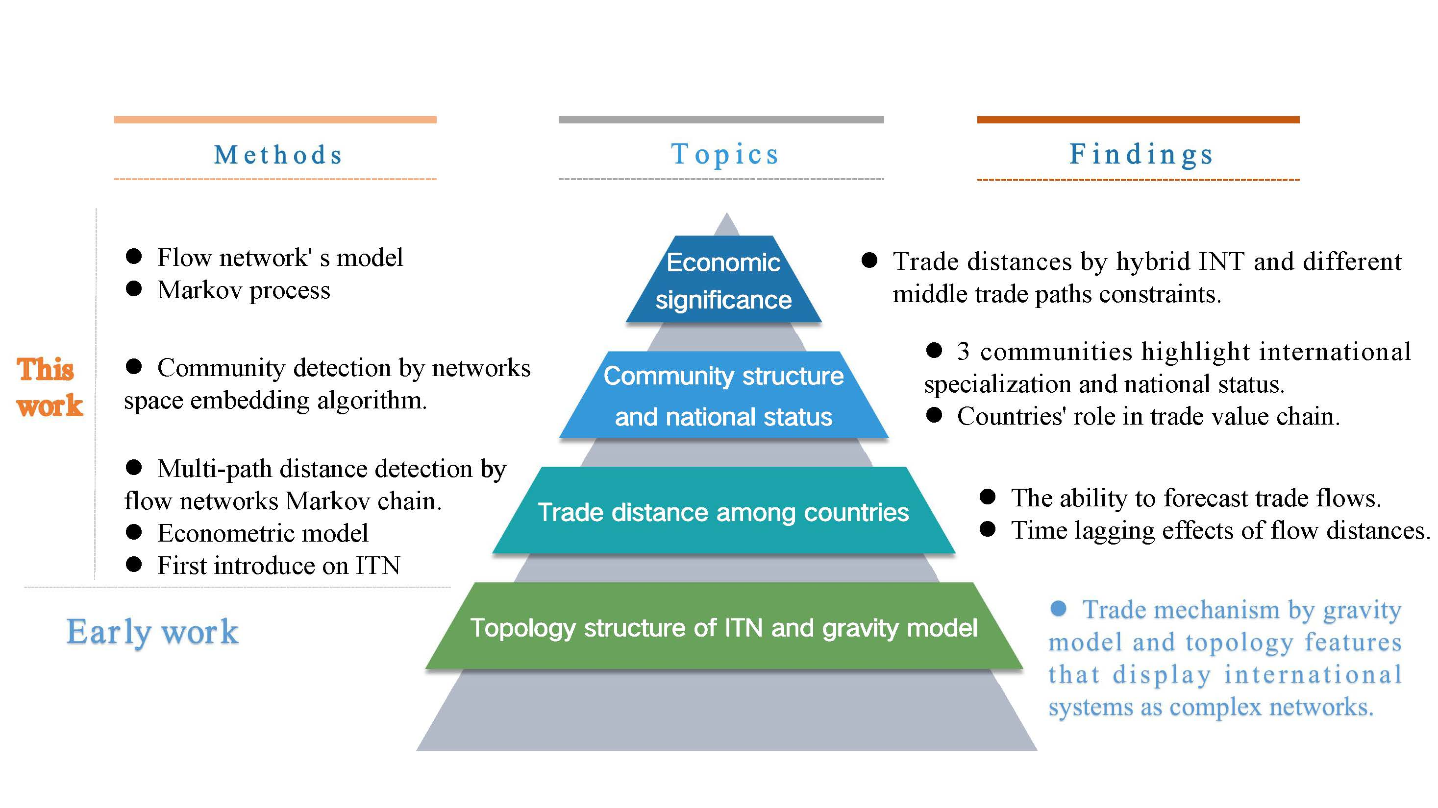
The international trade flow network F is a weighted directed network with nodes: N countries and two special nodes (i.e., the source (labeled “0”) and the sink (labeled “”), as shown in Figure 1A. The most significant difference from complex network models is that flow network models have two special nodes which represent the effect of the environment on the international trade systems. Specifically, the outflow from the source to a country is the domestic production within this country, and the inflow to the sink from a country is its domestic consumption, as shown in Figure 1A by the dashed arrows.
In the ITFN system, the relationships between a country and the two special nodes are defined by network balance principle: the total in-flow of each node equals its total outflow except for the sink and the source, i.e., . In some cases, the data for domestic productions and consumptions are not available. We replace these flows as the non-balanced trade flows. If a country’s total import value is larger than the total export (i.e., ), the net import can be the surrogate as the domestic consumption: the flow from i to the sink (i.e., orange dashed lines in Figure 1A). The net export represents the countries’ production: the flow from the source to i (i.e., green dashed lines in Figure 1A). By doing this, the element in the adjacency matrix of the flow trade network F is obtained, as follows:
where is calculated from the raw trade data: if a country i exports to a country j with trade volume , the element of adjacency matrix is set as , otherwise . According to to the raw trade data, the adjacency matrix F is shown in Figure 1A.
3.3. Flow Distances
Bilateral trade, such as commodity trade and capital flows, may increase due to the reduction in spatial distance costs, and the relationship between trade costs and trade flows remains a significant issue. International trade is not only subject to economic scale and geographical distance, but also the result of searching for trade information in various economies. The network information provides new perspectives and ideas for further detailed estimation of trade costs and trade flows. Based on the structure of international trade networks and trade flows, we employ flow distance to quantify effective distance in energy trade systems. Flow distance measures the relative trade flows between two countries. More specifically, following the insights of Guo [44], we briefly review how to get flow distance based on the flow network structure. First, all possible paths from i to j can be defined as
where is the probability that nodes (i.e., countries) transfer from i to j after k steps and satisfies . Thus, can be expressed as
where, the total flow can be calculated as [45], the inverse of M’s Laplacian is , is the element of the matrix U, and is the first-passage flow from the source to i. The number of nodes that jump from i to j along all possible paths with k steps is . M is a Markov matrix and its the element is
where represents the probability of nodes jumping to j if they are at i.
Note that all possible paths from i to j may contain the path from j to j during the random walk. Therefore, the definition of flow distance is represented as and the symmetric flow distance can be finally determined by
3.4. Quantifying Trade Barriers Based on Trade Flows
In a broad sense, measuring the effective trade distance is an approach to study international trade barriers. Many Non-Tariff Trade Barriers (NTBs) cannot be directly quantified, including technical regulations, quotas, subsidies, and some anti-dumping measures. Some authors attempted to quantify these NTBs by utilizing the price wedge method [46], but they suffered from difficulties in data acquisition as well as inconsistency of price data [17]. The most direct impact of NTBs is to modify the production conditions and costs in import and export countries and intermediate product manufacturers, thereby affecting the relative enterprises. It causes the change of products’ comparative advantage, due to the eventual alternation of advantageous industries and technologies. The alternation will be reflected in international trade [2,3]. Thus, some studies used trade flows to quantify barriers, e.g., quantitative tool method [47].
The international trade system is complex under the interaction of politics, trade barriers, and the games of national interests. Complex network methods are one of the most important tools in the study of a complex system. Such a method provides a global perspective to model the international trade system. The international trade network is stable [33], which offers the possibility for predicting future trade behavior by historical data. Intuitively, trade data are a process of coevolution between trade status and trade barriers. Just as the river shapes the bed while the bed, in turn, guides the flow, they constitute a complex system of coevolution. Because of the dependence on the path and the lock-in effect (i.e., stability over time) of the international trade network, the national trade behavior will be affected by the inherent network effect when the trade network space is formed. Trade behavior in the past determines the basic framework of the whole trade network space, which constrains the formation of the future space. Therefore, network constraints provide an internal basis for depicting trade barriers using historical data.
National trade behavior constructs an international trade network with the characteristics of complexity, nonlinearity, and time-varying under the constraints of all kinds of barriers. The potential information of trade resistance is thus hidden in trade network data, which makes it possible to quantify trade barriers. The quantification of effective trade distance aims to extract hidden resistance information from trade network data, including multilateral resistance and network effect. It needs to be reiterated that the restriction of economic behavior by resistance or barriers makes national trade behavior controlled by multilateral resistance, and accordingly the network effect. In general, the economic network is also understood as the result of a game between the subjects of competition and cooperation [48]. Thus, the trade network contains not only trade factors but also multi-dimensional information. In this paper, flow distance is adopted as the general measure quantify the trade barrier and multilateral resistance.
3.5. Econometric Methodology: Gravity Model
To understand the role of trade distance, it is mandatory to analyze all kinds of products trade and establish trade gravity models to compare. To examine the effectiveness of the flow distances, we employ the gravity model to compare the performance of geographical and flow distance. We select d GDP and distance (flow distance and geographical distance) as explanatory variables. The logarithm equation is converted into a linear form firstly, and the trade gravity model is expressed as follows: Model 1 (classical gravity model) and Model 2 (modified gravity model).
Model 1 is expressed as follows:
where measures the volume of bilateral trade from country i to country j, is the geographical distance between countries, denotes GDP of country i, and are fitting parameters.
Similarly, Model 2, the flow gravity model, is expressed as follows:
where is the flow distance among countries. Considering endogeneity, we adopt the rolling window method to consider the distance measure, that is, the flow distance generated by the historical trade data, to predict the current trade flows. is a time delay parameter, and flow distances of and predict the trade flow at time t.
4. Results
4.1. The Flow Distance in Energy Trade Networks
4.1.1. The Economic Meaning of Flow Distances
With the improvement of global value chain systems and the coupling interaction of international division of labor and transnational corporations, the national attributes of product sources are becoming increasingly vague, and it is difficult to identify the real producer from imported products and even to quantify such trade distances. From the perspective of the theory of the global value chain, the more complex the products are, the more processes are involved in the production, which makes trade distances in the commodity trade flow also contain potential multilateral paths.
Broadly speaking, the process of summation in this way reveals the potential trade distance of multi-path fusion behind the trade, which is fundamentally different from geographical distances. By contrast, the geographical distance of the classical gravity model cannot identify multilateral distance and the complexity caused by network effects, and the mechanism of trade flow cannot be described completely. More significantly, definition of distance which ignores the multilateral distance will seriously underestimate (that is, the blue area in Figure 1B) or overestimate (that is, the red area in Figure 1B) real trade distances.
Next, we illustrate the potential impact of multilateral goods trade on the “effective trade distance” with a simplified diagram of international trade relations in Figure 1A. First, geographical distances may understate effective trade distances. For instance, when measuring the trade distance between countries A and C, geographical distances only focus on the direct distance. However, there are three potential routes for commodities: A exports to C directly; A exports to C via B; and A exports transfer selling internally and re-exports to C. In doing so, the trade distance between A and C in Figure 1A is completely depicted as , which includes intermediate products imported from A. Second, geographical distances may overestimate effective trade distances, especially if A and E have important import and export relations with each other. When measuring trade distances between A and E, it cannot be avoided that E imports products from A and re-exports them to A. Thus, is calculated by Equation (6).
4.1.2. The Role of Flow Distance in the International Trade
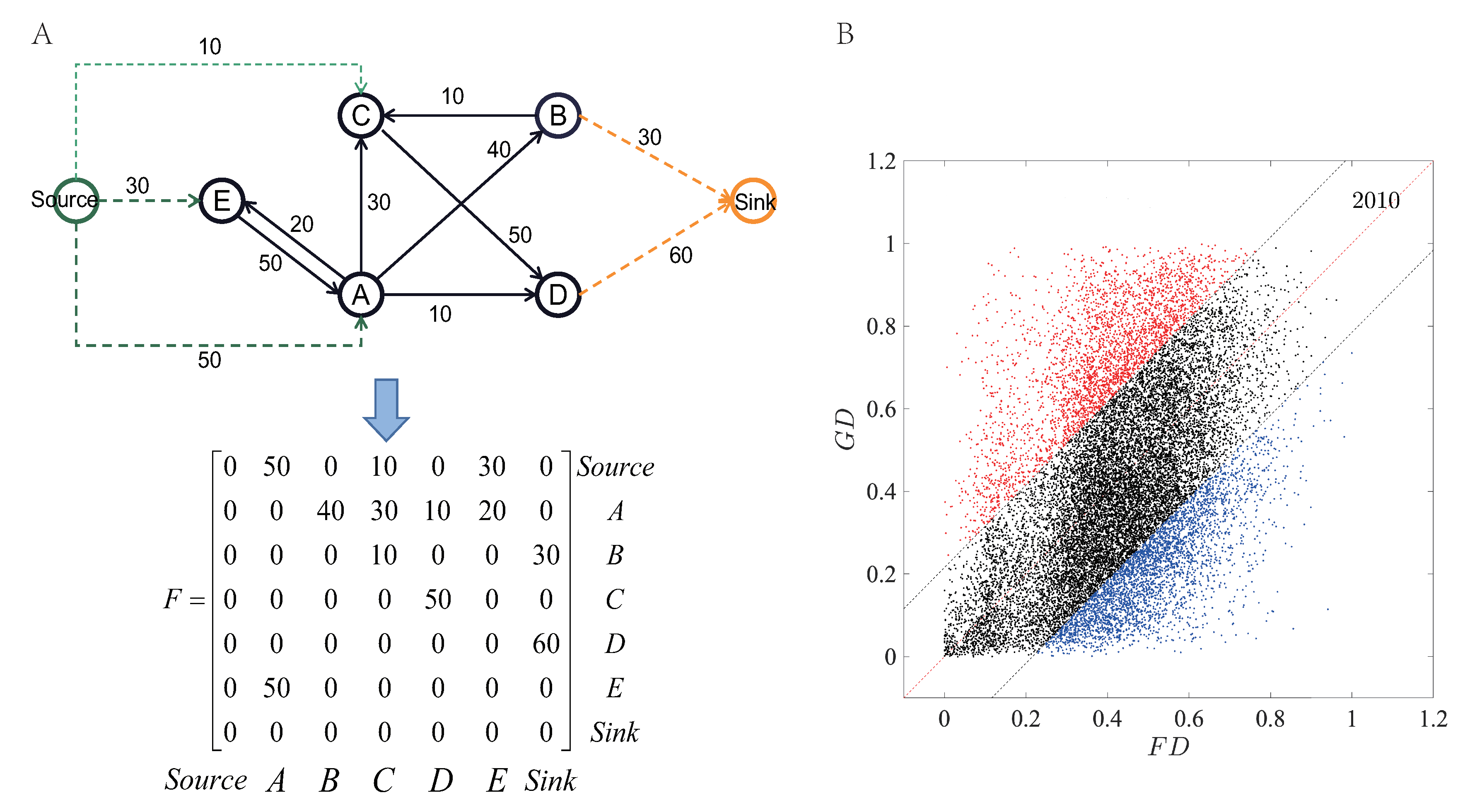
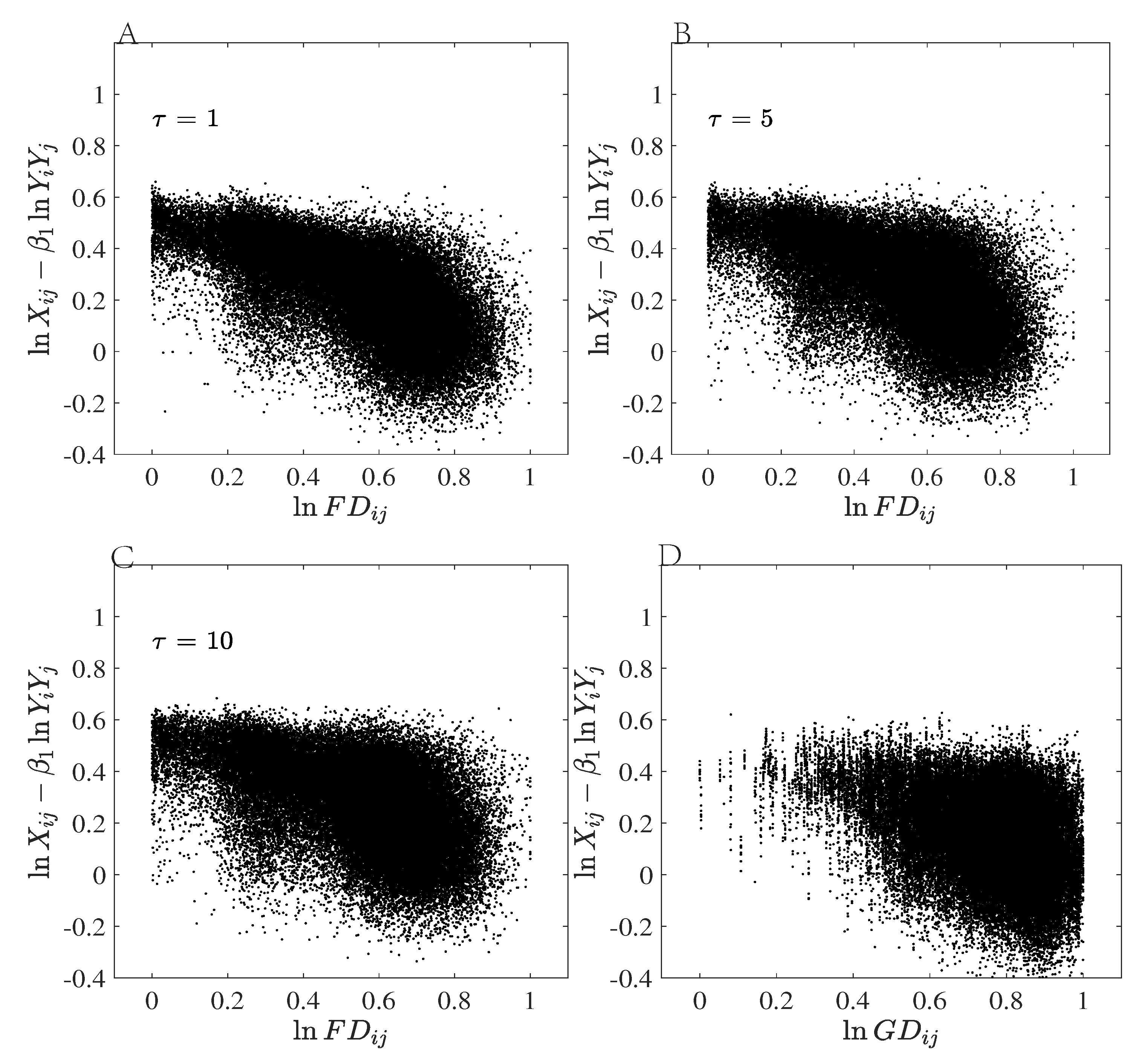
In this section, a detailed analysis focuses on the performance of flow distances to predict trade flows. To avoid endogeneity, we use a lagging distance variable (that is, flow distances with time delay feature) to replace the geographical distance in the classical gravity model. In doing so, flow distances at time are used as effective trade distance to predict trade flow at t time, and the flow distance under different delay coefficients are compared with the regression results of geographical distance. A more intuitive comparison scheme is first adopted. We plot logarithmic distance both for geographical (Figure 2D) and flow distances with (Figure 2A–C) against (the item of non-distances).
Here, for the sake of presentation, we mainly show the empirical results of the energy trade. When the delay variable is one or five years, the result of the forecast in Model 2 is significantly better than the measurement of geographical distance, i.e the scatters formed by the distance and non-distance terms are in the vicinity of a straight line. The result of the GDP regression coefficient is stable and significant under different flow distances with different time lags, and regression coefficients of flow distances in regression equations are always larger than the geographical distance, showing that effective distance (flow distance) has a stronger negative effect on trade flow than geographical distance. More generally, we do an empirical analysis of different products in different years and we can obtain similar results.
With the increasing value of time delay variable, the effect of flow distance will gradually degenerate into the role of geographic distance, which indicates that flow distance covers a wider range than geographic distance. In rough terms, the regression effect of geographic distance in the classical gravity model is equivalent to flow distances measured by trade networks over a 10-year delay, which has an obviously huge impact on trade flow forecasts, because the international situation is changing rapidly. Due to the path dependency and lock-in effect in the international trade system, when the new network space is formed, countries’ trade behaviors will be affected by the network. Thus, the network space and the trade flows co-evolve: past trade behaviors will determine the entire trade network space and future trade flows will be created by the existing trade network space. This understanding may help us revise the distance itself as the “effective distance” in the network space, rather than patching up the gravity model by adding factors.
Moreover, we also analyze the goodness of fit () in the regression model. In Table 1, the result shows that the gravity model with flow distance is accompanied by a higher . Specifically, taking the energy trade as an example, is between 0.50 and 0.53 in Model 2 with , while it is between 0.25 and 0.30 in Model 1. Flow distance has a better performance in all cases, which means that the gravity model can still explain international trade, but the geographical distance is insufficient to identify effective trade distance under multilateral trade resistance and multi-path effects. The regression results of different products and years are qualitatively consistent.
In this section, we show that better performance of gravity model can be derived by replacing the geographical distance with this new effective distance, which means the bilateral trade flows and the flow distances have much stronger correlations than the geographical distances. This phenomenon is robust against different products and different periods.
4.1.3. The Relationship between Flow Distance and Geographical Distance
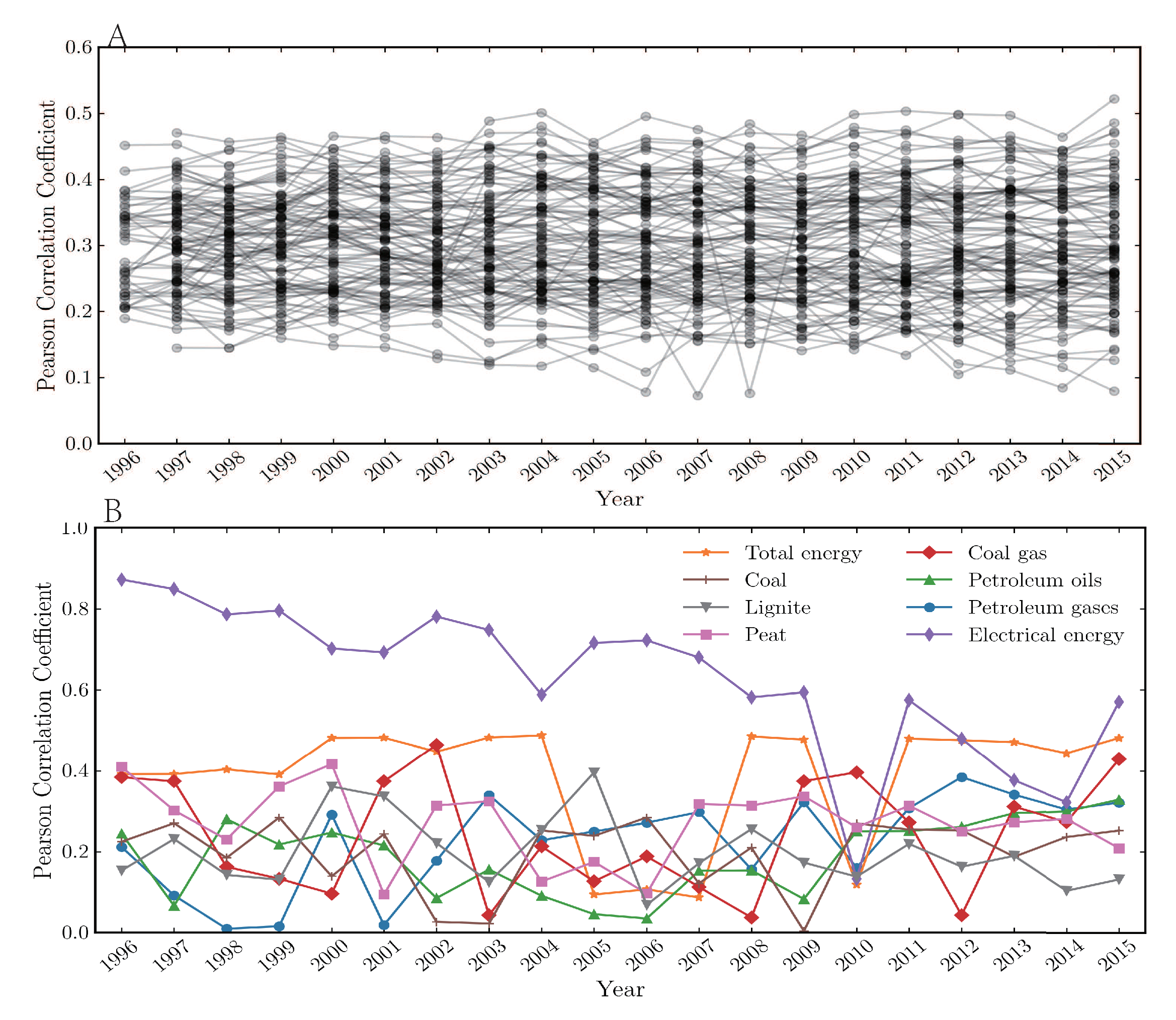
Time lag effect (that is, flow distances can degenerate into the effect of geographic distance with an adequate value of time delay) indicates that geographic information is hidden in flow distances from another perspective. It is a common understanding that trade distances embed geographical information and other information. Placed in the historical perspective, effective trade distance can be explored further by analyzing the dynamical Pearson correlations between flow distance and geographical distance in all products trade (a total of 97 products). The result is shown in Figure 3; for the most commodities trade, we can observe that the Pearson correlation coefficients are not significant in all periods, and their values are less than 0.5. This also indicates that the effective trade distance is mainly affected by trade structures and other network factors.
To highlight this effect, we further analyze the more detailed product classification of trade data. Illustrating by the case of energy, similar results have been captured by empirical data. The result is shown in Figure 3. It is worth mentioning that there is a weak sign that there aew geographical effects in the electricity trade. In the 1990s, the correlation between flow and geographical distance was as high as 90% in the electricity trade network, which indicates that geographical was the main influencing factor for trade flow. However, it is clear that the correlation continued to drop, which reveals that some other factors of distance gradually occupy the main position in affecting the trade volume.
In this section, we further discuss the relationship between flow distance and geographical distance. The results show that the trade distance generated by the embedding space includes geographical factors. Similar conclusions have been verified on different types of trade products.
4.2. Quantifying Community Structures and the National Status
4.2.1. Community Structure Detection by Flow Distances
Community structure is not only an important property for the complex network but also an important approach to depict the structure of economic systems. A network can be divided into several groups so that each group is tightly knit with many links inside, and there are only a few edges between each group [49]. The early research structure indicates that the community structure has the geographic aggregation feature, while the role of globalization has led to an unprecedented division of labor and links in the trade market, which in turn has produced heterogeneity of products, namely that differences in the added value of products [39]. Specifically, some high-end products, such as cars, can be split into different parts (intermediate products) and coordinated by various countries for production and assembly, which requires intermediate products, not for final consumption, but high value-added and export reproduction.For some agricultural and sideline products, on the contrary, imported products are mainly used for domestic consumption and their added value may be lower than some intermediate products [50,51]. From this view, we want to further discuss i the role of flow distance by considering multipath features in reshaping the international trade structure. Does international trade specialize in the production value chain or geographic aggregation? We expect to see communities form around international specialization and geographic aggregation, respectively.
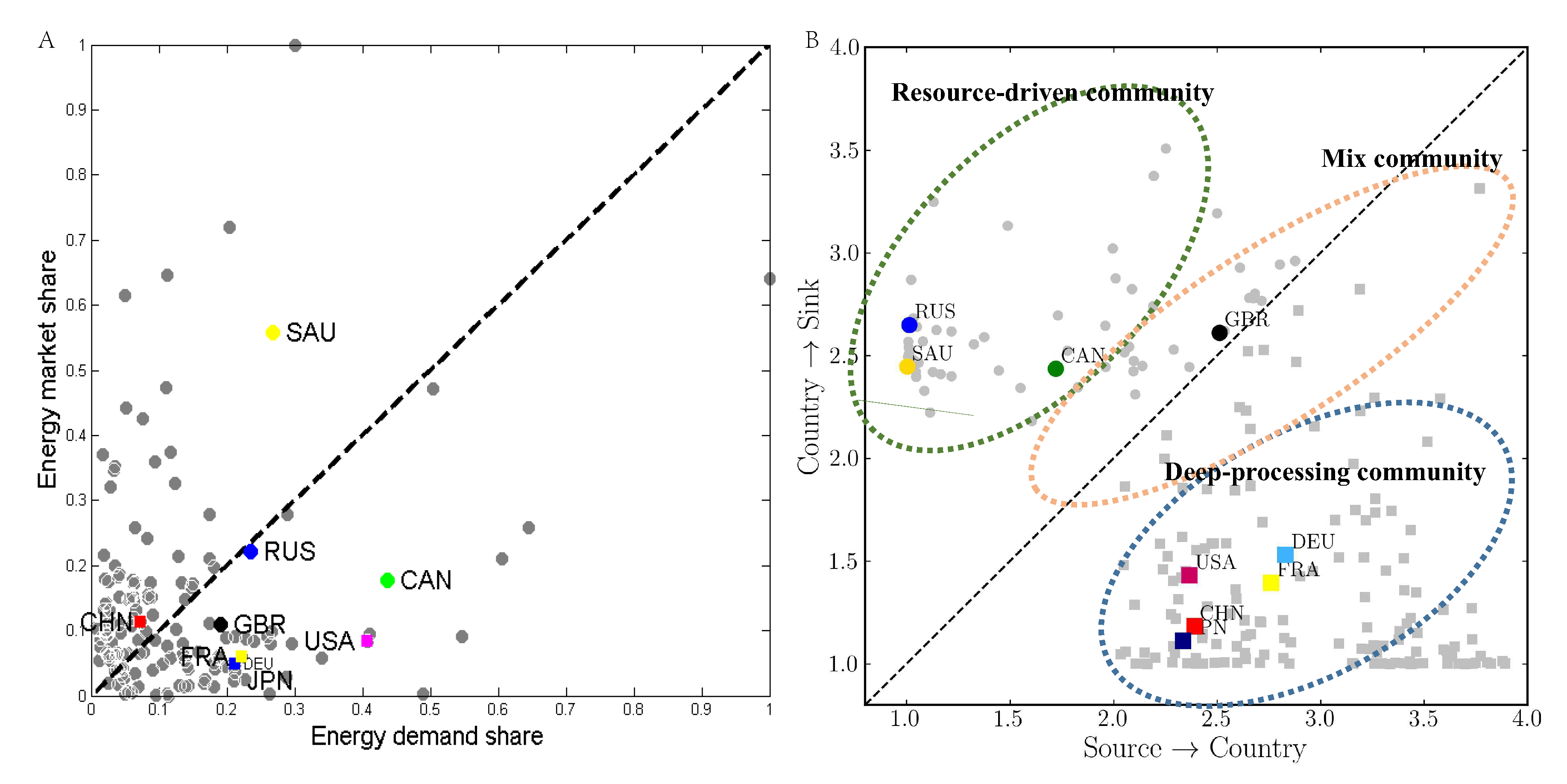
Next, we introduce a network flow space embedding model to detect the international trade network of community structures. The community division method by flow space embedding is based on the above two special flow distances to embed the entire trade network into a two-dimensional plane with the two kinds of distances as the axes (the country-from-the-source distance (s2c) as the horizontal axis, and the to-the-sink distance (c2s) as the vertical axis). It is noted that there are two special distances for each country. If a country has a shorter flow distance from the source, it is more likely to be a supplier of the energy product. Otherwise, the smaller is the flow distance to the sink, the higher is the propensity for the country to be a consumer of the energy product. Figure 4 shows that not all countries are on the diagonal of the s2c–c2sdistance plane. Namely that the national energy trade’s consumption and production status are not equal and the diversity exists in the form of a contribution to the energy value chain. Specifically, if the country’s y coordinate (c2s) is smaller, it is more likely that a consumer for the energy product locates at the high end of the energy production chain (i.e., the colorful dot points below the diagonal in Figure 4). Correspondingly, the lower is the x coordinate, the smaller is the s2c distance, and the greater is the propensity of the country to be an energy producer, and, thus, it locates at the low end of the energy production chain (i.e., colorful points above the diagonal in the Figure 4).
In doing so, three communities can be obtained by identifying the national energy consumption and industrial development level, including resource-driven community, deep-processing community, and mixed community. Note that Countries in the mixed community (related balance of trade) are also referred to as the trade balance or the international trade balance, which shows that the national status of import and export are roughly equal. BOT country corresponds to the black point in Figure 4. More precisely, countries above the diagonal line are natural resources abundant, such as Canada, Russia, and Saudi Arabia, and most of them are mainly exporters, who can maintain national economic stability by exporting energy. Their distances to the source are less than to the sink, therefore they locate at the bottom of the production chain. On the contrary, some countries are located below the diagonal, which are mainly energy importers. Their distances to the sink are lower than to the source; therefore, they are at the top of the production chain. Such countries tend to be lack of natural resources, such as Japan, and primary energy can be further processed to improve product competitiveness through importing. Finally, there are a few countries located near the diagonal, such as Britain.
To illustrate the validity, we furthermore provide the community structures of economic data by energy market share and demand share in Figure 4A. The results show that the flow distances plane can categorize the characteristics of international status clearer than the market and demand share. The energy market share and demand share are measured by the value of energy net exports and domestic energy use (kg of oil equivalent per capita), respectively. Especially, Russia and Canada fail to be effectively identified in the resource-driven community. Although the input–output structure and relative magnitude of production among sectors are not explained by trade status only, the theory of complex economy points that there are many unmeasurable factors, including infrastructure, education, vocational skills, and other factors, hidden behind economic behaviors. Those non-monetary metrics, based on trade network structures, have greatly enriched the theory of economy. Those unmeasurable factors are thus reflected in the country’s export capacity, i.e., trade data.
Actually, the s2c–c2s distances plane also provides us with a representation of the entire trade systems. This method shows the different community nature from that of traditional methods. The flow distances abstracted from trade networks embodies strong and stable explanatory power in describing multilateral trade distance to uncover the intrinsic structure of trading systems. Each type of international specialization in the production value chain also reflects the aggregation of national energy roles, rather than geographical clustering.
4.2.2. Identifying National Status in Trade Value Chain
In the analysis above, we verify that flow distance has better performance in explaining trade volume and representing hierarchical structures. From the perspective of the flow distance, the community structure of trade networks is driven by the coevolution of product specialization and geographic distance. Flow space embedding method not only can detect the community structure but also can reveal the position of the countries on the energy production chain according to their production chains and the level of added-values. To show this, because energy production, processing, and consumption are so important for countries in the sense of economics and politics, let us take the energy products as examples to show the flow distances.
In terms of countries with rich energy resources, such that they are major energy export countries, including Russia, Canada, Saudi Arabia, etc., their industrial structure is highly dependent on energy trade, therefore they often have some problems such as monotonous industries, lagging industrialization, and weak manufacturing development. For the oil trade market, in particular, resource-driven statehood makes the country become an important exporter of oil in the world. As an “oil country”, Saudi Arabia’s oil reserves and production are adequate in the world, and the petroleum and petrochemical industries are the blood of the country’s economy, and thus its contribution to the energy value chain is low.
Beyond that, we can identify countries’ capabilities with deep processing and high value-added product contribution. On the one hand, the deep-processing country would balance national demand through importing enough energy, which can be further processed to primary energy to produce higher value-added products. We can find that the developed countries have higher c2s distances in most commodity trades with countries, such as Japan, Germany, France, etc. These countries are located above the diagonal, which shows they can produce higher energy value. On the other hand, owing to resource emptiness, energy policies, etc., some countries flood into the energy consumption market. For instance, the United States has always had a protection policy for its domestic energy sources, relying on large amounts of imports to maintain domestic demands. The situation of coal is on the contrary. The United States and Australia are the world’s largest coal exporters, which confirms that the results of our energy flow distance can be used to identify the country’s position. China’s coal trade has similar phenomena.
Based on our results, we conclude that the distances of open flow systems can characterize the international status and value-added contribution capacity of a given country, which reveals that flow distances have economic significance. When the energy needs more complex production processes and energy demand, more countries must be imported from to form a long c2s distance. Thus, a longer national energy value chain is formed. As a method to quantify the energy national status, the flow distance can provide a new study perspective on related research.
4.2.3. The Evolution of the National Status in Energy Value Chain
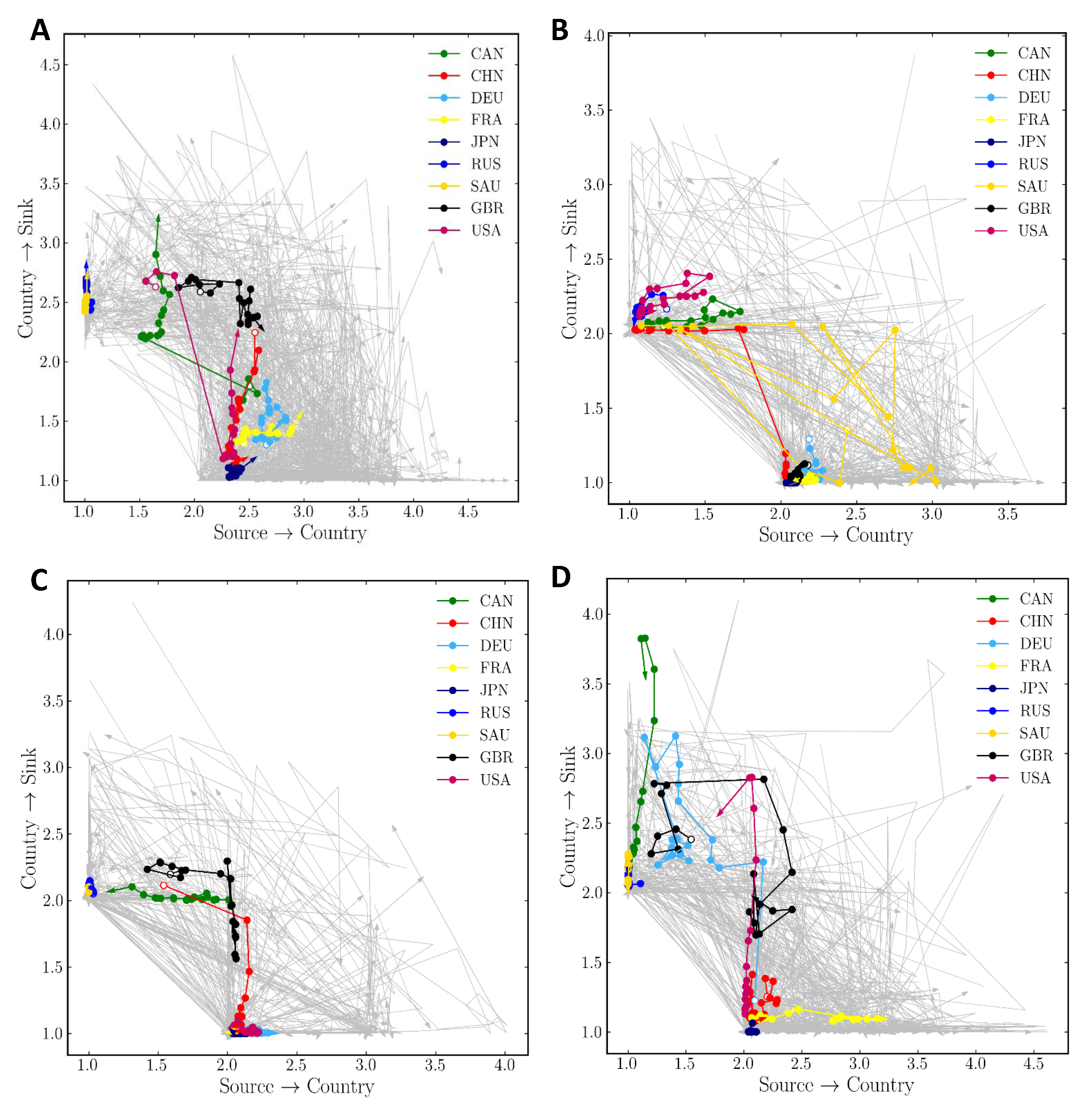
According to the observations, we know that flow distance is the basic property of national status and contributions of the products in the value chain. We expect countries with smaller c2s distance can produce more diversified products. Based on the evolution of c2s distance, we can trace the national development process. Similarly, for the evolution of s2c distance, we can find the development trend of national status and potential contributions. Therefore, the features of the evolution of national status are the key point of our analysis in the s2c–c2s distance plane. This section shows how the global production and consumption of energy trade evolve and the results are shown in Figure 5.
The three major energy resources, namely coal, oil, and natural gas, are in the core positions in the energy trade system. As an example, we analyze China’s evolution of production and consumption in the following part (that is, the red line in Figure 5). The c2s distance of coal has a huge reduction in 2008 and has been in a low state, which reveals that China’s coal processing level is relatively higher in the upstream industry chain. Meanwhile, it coincides with a significant increase in China’s coal inventories, which may confirm that China is moving to the “source”. Furthermore, China’s s2c distance is higher than the c2s distance in the oil trade flow network, and the flow distance from the source node is closer. Especially, China had reversed the way of the trade from oil exporter to oil importer country in 1996, after which China’s oil imports and dependence on foreign oil is gradually increasing. Besides, the natural gas trade in Germany and the United States fluctuates, while China, Russia, Japan, and Saudi Arabia are relatively stable.
Another interesting finding is that studies based on flow distance have detected that China, Britain, Africa, and other places inject new vitality into the energy market. For example, the black line in Figure 5 shows that the UK’s energy consumption capacity has gradually increased since 2005, and the main reason is the depletion of North Sea oil fields, which led to the failure of the UK energy industry’s self-reliance. More importantly, Britain’ s2c distance of electricity trade has been higher than c2s distance since 2008. It is obvious that, as the first country to complete the industrial revolution, Britain also changes from the direction of energy consumption to clean energy in the process of development.
In this section, taking the energy trade as an example, we explore the evolution of the national status by flow distance using the trade flow network model. The results show that the trade distance of network structure and multi-path coupling not only predicts trade flow well but also has an important meaning to shape the trade network structure and the position of the country in the trade value chain.
5. Discussion
We propose trade distances by focusing on multilateral trade path and network effects emerging from trade relations to formulate a general model describing the effective distance of trade. By studying the properties of the flow distances, we find that structure-based flow distance can better explain the motivation of trade volume in the gravity model. Flow distance can be considered as an effective distance of trade to quantify the diversity of distance in bilateral trade.
In the first analysis, the gravity law can be supported by the empirical data if the geographical distance is replaced by flow distance. Regression results of flow distances are all significantly greater than those for geographical distance, which shows that the flow distance is more suitable for quantifying the effective distance of international trade. The correlation between flow distance and geographical distance also reveals that trade distances encode more than purely geographical information. Noteworthy, compared with hyperbolic distance and Brockman’s effective distance, flow distances reflect the heterogeneity of the international trade network by incorporating the trade network topology and the flow information of the nodes together. Hyperbolic distance is defined as “effective distance” by incorporating the trade network topology and the GDP information of the nodes together [31,52]. Although it obtains a better description for the international trade network, the trade flow information is not contained in this distance; therefore, it is difficult to represent the rich information of the multi-lateral trades encoded in paths. Brockman’s effective distance only calculates the distance of the maximum likelihood paths between nodes [32], but does not count all paths. Importantly, trade distances may consider how national behavior across the trade value chain acts on international trade, including direct and indirect effects.
In the second analysis, experimental evidence finds that flow distance can collapse to the predicted results of geographic distance with the appropriate time lagging variable. Due to the path dependence and lock-in effect in the international trade system, when the new network space is formed, countries’ trade behaviors will be affected by the network. Past trade behaviors will determine the entire trade network space and future trade flows will be created by the existing trade network space. This understanding may help us to revise the distance itself as the “effective distance” in the network space. Some advantages of the effective distance, which is defined by using the historical trade network data, are as follows. From the perspective of topological structure, the international network is relatively stable within a certain range [53], which reflects the hypothesis of statistical stationarity in economics. Especially, the trade structure may not be changed suddenly by trade policies in the short term, because the role of economic policies has the property of time lag [54]. It provides the basis for the flow distance prediction of short-term trade. Additionally, the complex network model is more intuitive to portray multilateral trade resistance, since it considers international trade as a whole. With the increase of the time lag parameter in Equation (7), the prediction of the flow distance to trade flows gradually degenerates into the effect of geographical distances. Furthermore, the mechanism of flow distances has yet to be explored. How flow distances reshape trade architecture and organizations can be discussed.
In the third analysis, using the theoretical model of international trade, the forming mechanism of the international trade network is further discussed. The global value chain is changing the world trade pattern, and the flow network model also shows the formation of the trade value chain of commodities at the macro and micro scales in international trade. In this paper, we use the flow-space distance embedding scheme to detect the community structure in international trade networks. The classic community detection algorithm is to classify countries through the maximum modularity function Q [55,56]. A larger value of Q indicates a better division effect. Different from previous literature, the community division method by flow distances embedding highlights the function of the country in the energy value chain. From an evolutionary perspective, as shown in Figure 5, the countries within the community are relatively stable, but some large countries have changed greatly. The community structure obtained by the optimization method has the effect of geographical agglomeration and has a prominent position in Asia over time [13,57]. However, this community division method is coarse-grained. How to explore a more refined algorithm may be an important field in future studies.
6. Conclusions
Complex network models provide a snapshot of international trade systems, enabling us to understand international trade as a whole and analyze the issues of trade in a multi-level view. For trade distances, a simple and effective method is used by us to detect the national status and analyze the trade distances through the mobility of international trade. In this paper, we first construct trade distances by focusing on multilateral trade path and network effects emerging from trade relations according to the trade flow network structure and commodity flows. Next, we verify that the flow distance defined above is reasonable and effective, using an econometric methodology, namely gravity model. Finally, we link the effective distance to the economy. The results show that flow distance is an effective classification of the country’s position in the energy production value chain.
Author Contributions
Conceptualization, J.Z. and H.C.; methodology, Y.F. and Z.D.; software, R.Z. and Z.W.; validation, R.Z., J.Z., and Z.W.; formal analysis, Z.W. and H.C.; investigation, Z.W.; resources, Y.F. and J.Z.; data curation, Z.W. and R.Z.; writing—original draft preparation, Z.W. and J.Z.; writing—review and editing, Z.W. and J.Z.; visualization, Z.W.; supervision, Z.D. and J.Z.; nd funding acquisition, all authors. All authors have read and agreed to the published version of the manuscript.
Funding
This research was funded the National Natural Science Foundation of China (NSFC, under the grant numbers Nos. 71731002, 61673070, 61573065, and 71773007), BNU Interdisciplinary Research Foundation for the First-Year Doctoral Candidates (Grant BNUXKJC1921), and Beijing Normal University Interdisciplinary Construction Project.
Conflicts of Interest
The authors declare no conflict of interest.
References
- Hausmann, R.; Hwang, J.; Rodrik, D. What you export matters. J. Econ. 2007, 12, 1–25. [Google Scholar] [CrossRef]
- Hidalgo, C.A.; Klinger, B.; Barabási, A.-L.; Hausmann, R. The product space conditions the development of nations. Science 2007, 317, 482–487. [Google Scholar] [CrossRef] [PubMed] [Green Version]
- Hidalgo, C.A.; Hausmann, R. The building blocks of economic complexity. Proc. Natl. Acad. Sci. USA 2009, 106, 10570–10575. [Google Scholar] [CrossRef] [PubMed] [Green Version]
- Tacchella, A.; Cristelli, M.; Caldarelli, G.; Gabrielli, A.; Pietronero, L. A new metrics for countries’ fitness and products’ complexity. Sci. Rep. 2012, 2, 723. [Google Scholar] [CrossRef] [Green Version]
- Matthieu, C.; Andrea, G.; Andrea, T.; Guido, C.; Luciano, P.; Alain, B. Measuring the intangibles: A metrics for the economic complexity of countries and products. PLoS ONE 2013, 8, e70726. [Google Scholar]
- Brummitt, C.D.; Gómez-Liévano, A.; Hausmann, R.; Bonds, M.H. Machine-learned patterns suggest that diversification drives economic development. J. R. Soc. Interface 2020, 17, 20190283. [Google Scholar] [CrossRef]
- Popescu, C.R.; Popescu, G.N.; Popescu, V.A. Assessment of the state of implementation of excellence model common assessment framework (caf) 2013 by the national institutes of research–development–innovation in romania. Amfiteatru Econ. 2017, 19, 41–60. [Google Scholar]
- Popescu, C.R.G.; Popescu, G.N. An exploratory study based on a questionnaire concerning green and sustainable finance, corporate social responsibility, and performance: Evidence from the romanian business environment. J. Risk Financ. Manag. 2019, 12, 162. [Google Scholar] [CrossRef] [Green Version]
- Pöyhönen, P. A tentative model for the volume of trade between countries. Weltwirtschaftliches Arch. 1963, 90, 93–100. [Google Scholar]
- Leibenstein, H.; Tinbergen, J. Shaping the world economy: Suggestions for an international economicpolicy. Econ. J. 1964, 76, 92–95. [Google Scholar]
- Chaney, T. The gravity equation in international trade: An explanation. J. Political Econ. 2018, 126, 150–177. [Google Scholar] [CrossRef] [Green Version]
- Head, K.; Mayer, T. Gravity equations: Workhorse, toolkit, and cookbook. Handb. Int. Econ. 2014, 4, 131–195. [Google Scholar]
- Fan, Y.; Ren, S.; Cai, H.; Cui, X. The state’s role and position in international trade: A complex network perspective. Econ. Model. 2014, 39, 71–81. [Google Scholar] [CrossRef]
- Wu, Z.; Fan, Y. Review of international trade: The complex network approach. J. Univ. Electron. Sci. Technol. China 2018, 47, 469–480. [Google Scholar]
- Blázquez Fernández, C.; Cantarero Prieto, D.; Pascual Sáez, M. Patient cross-border mobility: New findings and implications in spanish regions. Econ. Sociol. 2017, 10, 11–21. [Google Scholar] [CrossRef] [Green Version]
- Stavytskyy, A.; Kharlamova, G.; Giedraitis, V.; Sengul, E.C. Gravity model analysis of globalization process in transition economies. J. Int. Stud. 2019, 12, 322–341. [Google Scholar] [CrossRef]
- Anderson, J.E.; Van Wincoop, E. Trade costs. J. Econ. Lit. 2004, 42, 691–751. [Google Scholar] [CrossRef]
- Bergstrand, J.H. The gravity equation in international trade: Some microeconomic foundations and empirical evidence. Rev. Econ. Stat. 1985, 67, 474–481. [Google Scholar] [CrossRef]
- Bergstrand, J.H. The generalized gravity equation, monopolistic competition, and the factor-proportions theory in international trade. Rev. Econ. Stat. 1989, 71, 143–153. [Google Scholar] [CrossRef]
- Krautheim, S. Heterogeneous firms, exporter networks and the effect of distance on international trade. J. Int. Econ. 2012, 87, 27–35. [Google Scholar] [CrossRef]
- Eslava, M.; Tybout, J.; Jinkins, D.; Krizan, C.; Eaton, J. A Search and Learning Model of Export Dynamics. Soc. Econ. Dyn. 2015, 1535. [Google Scholar]
- Yi, K.-M. Can multistage production explain the home bias in trade? Am. Rev. 2010, 100, 364–393. [Google Scholar] [CrossRef] [Green Version]
- Lin, F.; Sim, N.C. Death of distance and the distance puzzle. Econ. Lett. 2012, 116, 225–228. [Google Scholar] [CrossRef]
- Yotov, Y.V. A simple solution to the distance puzzle in international trade. Econ. Lett. 2012, 117, 794–798. [Google Scholar] [CrossRef]
- Carrère, C.; De Melo, J.; Wilson, J. The distance puzzle and low-income countries: An update. J. Econ. Surv. 2013, 27, 717–742. [Google Scholar] [CrossRef]
- Larch, M.; Norbäck, P.-J.; Sirries, S.; Urban, D.M. Heterogeneous firms, globalisation and the distance puzzle. World Econ. 2016, 39, 1307–1338. [Google Scholar] [CrossRef]
- Maciejewski, M.; Wach, K. What determines export structure in the eu countries?: The use of gravity model in international trade based on the panel data for the years 1995–2015. J. Int. Stud. 2019, 12, 151–167. [Google Scholar] [CrossRef] [Green Version]
- Mendoza, R.U. Trade-induced learning and industrial catch-up. Econ. J. 2010, 120, F313–F350. [Google Scholar] [CrossRef]
- Keller, W. Are international r&d spillovers trade-related?: Analyzing spillovers among randomly matched trade partners. Eur. Econ. Rev. 1998, 42, 1469–1481. [Google Scholar]
- Amiti, M.; Konings, J. Trade liberalization, intermediate inputs, and productivity: Evidence from indonesia. Am. Econ. Rev. 2007, 97, 1611–1638. [Google Scholar] [CrossRef]
- García-Pérez, G.; Boguñá, M.; Allard, A.; Serrano, M.Á. The hidden hyperbolic geometry of international trade: World trade atlas 1870–2013. Sci. Rep. 2016, 6, 33441. [Google Scholar] [CrossRef] [PubMed]
- Brockmann, D.; Helbing, D. The hidden geometry of complex, network-driven contagion phenomena. Science 2013, 342, 1337–1342. [Google Scholar] [CrossRef] [PubMed] [Green Version]
- Fagiolo, G.; Reyes, J.; Schiavo, S. The evolution of the world trade web: A weighted-network analysis. J. Evol. Econ. 2010, 20, 479–514. [Google Scholar] [CrossRef]
- Kali, R.; Reyes, J. The architecture of globalization: A network approach to international economic integration. J. Int. Bus. Stud. 2007, 38, 595–620. [Google Scholar] [CrossRef]
- De Benedictis, L.; Tajoli, L. The world trade network. World Econ. 2011, 34, 1417–1454. [Google Scholar] [CrossRef]
- Foti, N.J.; Pauls, S.; Rockmore, D.N. Stability of the world trade web over time—An extinction analysis. J. Econ. Dyn. Control. 2013, 37, 1889–1910. [Google Scholar] [CrossRef] [Green Version]
- Serrano, M.Á.; Boguñá, M.; Vespignani, A. Patterns of dominant flows in the world trade web. J. Econ. Interact. Coord. 2007, 2, 111–124. [Google Scholar] [CrossRef] [Green Version]
- Lee, K.-M.; Yang, J.-S.; Kim, G.; Lee, J.; Goh, K.-I.; Kim, I. Impact of the topology of global macroeconomic network on the spreading of economic crises. PLoS ONE 2011, 6, e18443. [Google Scholar] [CrossRef]
- Shi, P.; Zhang, J.; Yang, B.; Luo, J. Hierarchicality of trade flow networks reveals complexity of products. PLoS ONE 2014, 9, e98247. [Google Scholar] [CrossRef] [Green Version]
- Nicolis, G. Self-Organization in Nonequilibrium Systems: From Dissipative Structures to Order through Fluctuations; Wiley: New York, NY, USA, 1977. [Google Scholar]
- Hannon, B. The structure of ecosystems. J. Theor. Biol. 1973, 41, 535–546. [Google Scholar] [CrossRef]
- Odum, H.T. Self-organization, transformity, and information. Science. 1988, 242, 1132–1139. [Google Scholar] [CrossRef] [PubMed] [Green Version]
- Zhang, J.; Guo, L. Scaling behaviors of weighted food webs as energy transportation networks. J. Theor. Biol. 2010, 264, 760–770. [Google Scholar] [CrossRef] [PubMed] [Green Version]
- Guo, L.; Lou, X.; Shi, P.; Wang, J.; Huang, X.; Zhang, J. Flow distances on open flow networks. Phys. Stat. Mech. Appl. 2015, 437, 235–248. [Google Scholar] [CrossRef] [Green Version]
- Higashi, M.; Patten, B.C.; Burns, T.P. Network trophic dynamics: The modes of energy utilization in ecosystems. Ecol. Model. 1993, 66, 1–42. [Google Scholar] [CrossRef]
- Deardorff, A.V.; Stern, R.M. Measurement of Non Tariff Barriers: Studies in International Economics; University of Michigan Press: Detroit, MI, USA, 1998. [Google Scholar]
- Francois, J.; Hoekman, B. Estimates of Barriers to Trade in Services; Erasmus University: Rotterdam, The Netherlands, 1999. [Google Scholar]
- Schweitzer, F.; Fagiolo, G.; Sornette, D.; Vega-Redondo, F.; Vespignani, A.; White, D.R. Economic networks: The new challenges. Science 2009, 325, 422–425. [Google Scholar] [CrossRef]
- Newman, M. The Structure and Function of Complex Networks. Siam Rev. 2003, 45, 167–256. [Google Scholar] [CrossRef] [Green Version]
- Carswell, G.; De Neve, G. Labouring for global markets: Conceptualising labour agency in global production networks. Geoforum 2013, 44, 62–70. [Google Scholar] [CrossRef] [Green Version]
- Kotha, S.; Srikanth, K. Managing a global partnership model: Lessons from the being 787 ‘dreamliner’ program. Glob. Strategy J. 2013, 3, 41–66. [Google Scholar] [CrossRef]
- Papadopoulos, F.; Kleineberg, K.-K. Link persistence and conditional distances in multiplex networks. Phys. Rev. E 2019, 99, 012322. [Google Scholar] [CrossRef] [Green Version]
- Fagiolo, G.; Reyes, J.; Schiavo, S. World-trade web: Topological properties, dynamics, and evolution. Phys. Rev. E 2009, 79, 036115. [Google Scholar] [CrossRef] [Green Version]
- Meng, H.; Xu, H.-C.; Zhou, W.-X.; Sornette, D. Symmetric thermal optimal path and time-dependent lead-lag relationship: Novel statistical tests and application to uk and us real-estate and monetary policies. Quant. Financ. 2017, 17, 959–977. [Google Scholar] [CrossRef] [Green Version]
- He, J.; Deem, M.W. Structure and response in the world trade network. Phys. Rev. Lett. 2010, 105, 198701. [Google Scholar] [CrossRef] [PubMed] [Green Version]
- Tzekina, I.; Danthi, K.; Rockmore, D.N. Evolution of community structure in the world trade web. Eur. Phys. J. B 2008, 63, 541–545. [Google Scholar] [CrossRef] [Green Version]
- Piccardi, C.; Tajoli, L. Existence and significance of communities in the world trade web. Phys. Rev. 2012, 85, 066119. [Google Scholar] [CrossRef]
Figure 1.
Flow complex network of energy trade. (A) International trade flows network diagram. Black solid lines denote the raw trade data, and dashed lines represent the trade gap between imports and exports. The source node and sink node make the country’s import and export trade in the balanced state, which helps the definition of a Markov matrix during the derivation of flow distances. (B) The plane rectangular coordinate system consisting of flow distance (FD) and geographic distance (GD). is the case where the flow distance is equal to the geographic distance. The black area in the picture is the range of standard deviation of a straight line . Blue and red represent the data points beyond the standard deviation range.

Figure 2.
The regression results of gravity equations. The x-axis is distance variable and the y-axis is a non-distance variable : (A–C) the results of Model 2 with different lag times; and (D) the results of Model 1.
Figure 2.
The regression results of gravity equations. The x-axis is distance variable and the y-axis is a non-distance variable : (A–C) the results of Model 2 with different lag times; and (D) the results of Model 1.

Figure 3.
Correlation analysis of flow distances and geographic distances: (A) the correlation coefficient evolution of flow and geographical distance in all products; and (B) the correlation coefficient evolution of flow and geographical distance in more detailed energy products.
Figure 3.
Correlation analysis of flow distances and geographic distances: (A) the correlation coefficient evolution of flow and geographical distance in all products; and (B) the correlation coefficient evolution of flow and geographical distance in more detailed energy products.

Figure 4.
The national status in the s2c–c2s distance plane for energy product in 2005: (A) the result of community structure of energy market share and demand share; and (B) the result of community structure based on flow distance.
Figure 4.
The national status in the s2c–c2s distance plane for energy product in 2005: (A) the result of community structure of energy market share and demand share; and (B) the result of community structure based on flow distance.

Figure 5.
The evolution of status and contribution of nations in the flow space: (A–D) the evolution of the status in the energy, coal, natural gas, and oil markets, respectively, for the years 1996–2015. The arrow indicates the country’s evolution direction in the two-dimensional plane. For each point in pictures, the position is determined by the S2C distance and C2S distance.


Table 1.
The mapping results of important properties. is the regression coefficient of the distance term, and all the model results are at the 0.01 significance level. is the fitting effects of regression equations.
Table 1.
The mapping results of important properties. is the regression coefficient of the distance term, and all the model results are at the 0.01 significance level. is the fitting effects of regression equations.
| Year | Model 1 | Model 2 | ||||||
|---|---|---|---|---|---|---|---|---|
| 2006 | 0.29 | −0.42 | 0.51 | −0.54 | 0.44 | −0.47 | 0.37 | −0.44 |
| 2007 | 0.28 | −0.41 | 0.5 | −0.53 | 0.44 | −0.5 | 0.38 | −0.43 |
| 2008 | 0.29 | −0.39 | 0.51 | −0.51 | 0.44 | −0.47 | 0.4 | −0.44 |
| 2009 | 0.29 | −0.4 | 0.5 | −0.53 | 0.43 | −0.47 | 0.39 | −0.45 |
| 2010 | 0.29 | −0.4 | 0.51 | −0.54 | 0.42 | −0.46 | 0.4 | −0.46 |
| 2011 | 0.29 | −0.42 | 0.52 | −0.55 | 0.42 | −0.48 | 0.39 | −0.44 |
| 2012 | 0.31 | −0.44 | 0.53 | −0.55 | 0.44 | −0.49 | 0.41 | −0.47 |
| 2013 | 0.29 | −0.42 | 0.53 | −0.56 | 0.44 | −0.49 | 0.4 | −0.44 |
| 2014 | 0.29 | −0.41 | 0.53 | −0.54 | 0.45 | −0.5 | 0.4 | −0.47 |
| 2015 | 0.29 | −0.41 | 0.52 | −0.53 | 0.47 | −0.51 | 0.4 | −0.43 |
© 2020 by the authors. Licensee MDPI, Basel, Switzerland. This article is an open access article distributed under the terms and conditions of the Creative Commons Attribution (CC BY) license (http://creativecommons.org/licenses/by/4.0/).
Share and Cite
MDPI and ACS Style
Wu, Z.; Cai, H.; Zhao, R.; Fan, Y.; Di, Z.; Zhang, J. A Topological Analysis of Trade Distance: Evidence from the Gravity Model and Complex Flow Networks. Sustainability 2020, 12, 3511. https://0-doi-org.brum.beds.ac.uk/10.3390/su12093511
AMA Style
Wu Z, Cai H, Zhao R, Fan Y, Di Z, Zhang J. A Topological Analysis of Trade Distance: Evidence from the Gravity Model and Complex Flow Networks. Sustainability. 2020; 12(9):3511. https://0-doi-org.brum.beds.ac.uk/10.3390/su12093511
Chicago/Turabian StyleWu, Zongning, Hongbo Cai, Ruining Zhao, Ying Fan, Zengru Di, and Jiang Zhang. 2020. "A Topological Analysis of Trade Distance: Evidence from the Gravity Model and Complex Flow Networks" Sustainability 12, no. 9: 3511. https://0-doi-org.brum.beds.ac.uk/10.3390/su12093511
Note that from the first issue of 2016, this journal uses article numbers instead of page numbers. See further details here.