A DSGE-VAR Analysis for Tourism Development and Sustainable Economic Growth


1
Department of Economic Theory and History, Campus El Ejido, University of Málaga, 29071 Málaga, Spain
2
PhD Program in Tourism, Campus El Ejido, University of Málaga, 29071 Málaga, Spain
3
Department of Finance and Accounting, Campus El Ejido, University of Málaga, 29071 Málaga, Spain
*
Author to whom correspondence should be addressed.
Sustainability 2020, 12(9), 3635; https://0-doi-org.brum.beds.ac.uk/10.3390/su12093635
Submission received: 31 March 2020
/
Revised: 20 April 2020
/
Accepted: 28 April 2020
/
Published: 1 May 2020
(This article belongs to the Special Issue Innovation Management, Strategy and Sustainability in Tourism and Hospitality)
Abstract
:This paper aims to provide a better basis for understanding the transmission connection between tourism development and sustainable economic growth in the empirical scenario of International countries. In this way, we have applied the dynamic stochastic general equilibrium (DSGE) model in different countries in order to check the power of generalization of this framework to study the tourism development. Also, we extend this model to obtain the long-term effects of tourism development with confidence intervals. The influence of tourism development on sustainable economic growth is proved by our results and show the indirect consequences between tourist activity and other industries produced through the external effects of investment and human capital and public sector. Our study confirms that the DSGE technique can be a generalized model for the analysis of tourism development and, especially, can improve previous precision results with the DSGE-VAR model, where vector autoregression (VAR) is introduced in the DSGE model. The simulation results reveal even more than when the productivity of the economy in general enhances, as the current tourist demand increases in greater proportion than more than the national tourism demand. For its part, the consumption of domestic tourism rises more than the consumption of inbound tourism if the productivity of the tourism production enhances, but non-tourism prices decrease at a slower rate and tourism investment needs a longer time to recover to what is established.
1. Introduction
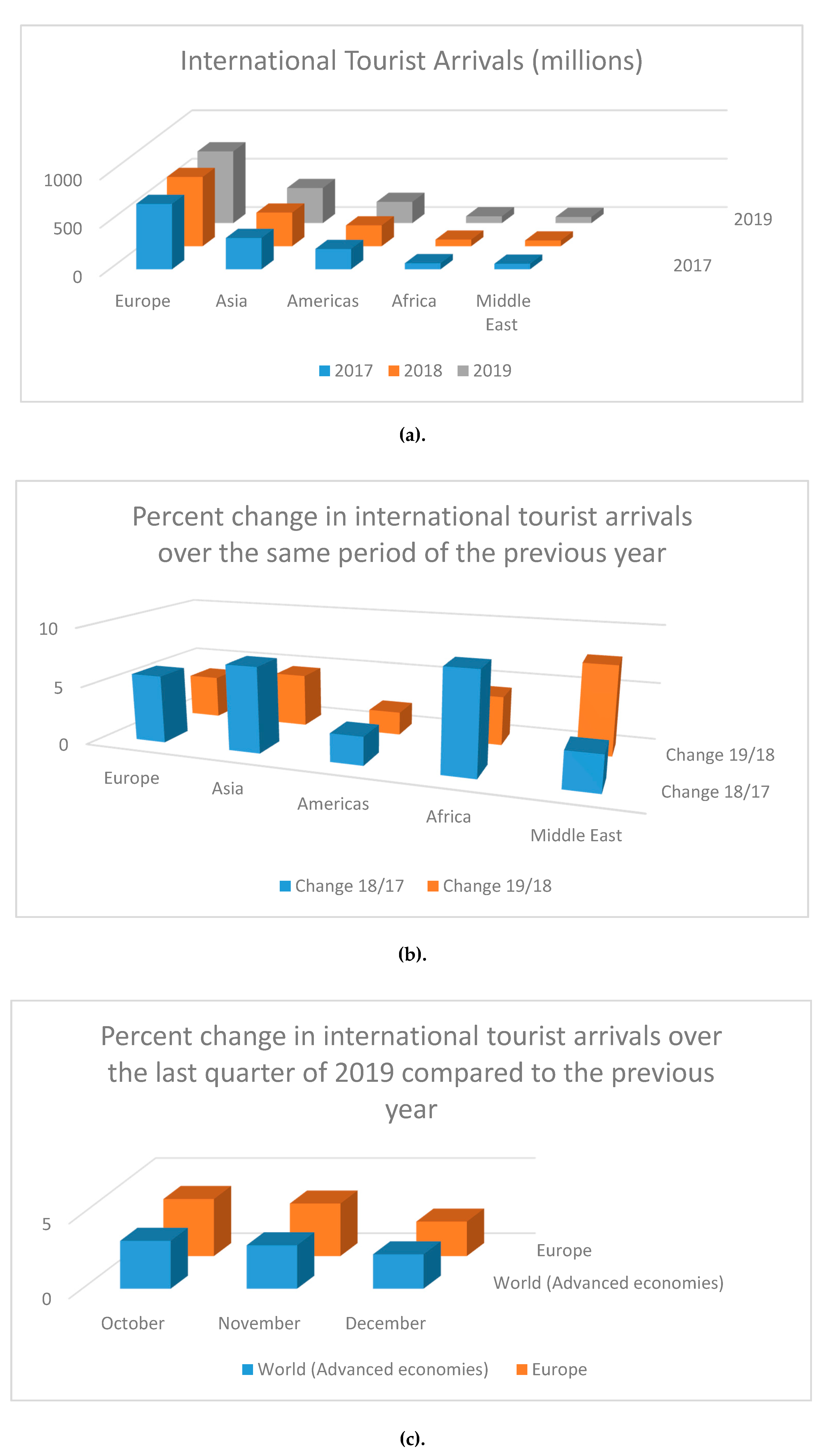
In recent decades, the tourism industry has established itself as a sector of great relevance to the world economy. According to data from the World Tourism Barometer [1], the tourism sector represented 6.8% of world economy every year. Despite being in a current environment of lower economic growth, this sector is resistant as its employment and consumer confidence levels continue to increase in 2019. In fact, following the same report, the international tourism arrivals have grown 4% in the first nine months of 2019, after 6% in 2018, and the international tourism receipts can be seen over a longer period in revenues from visitor spending (Figure 1).
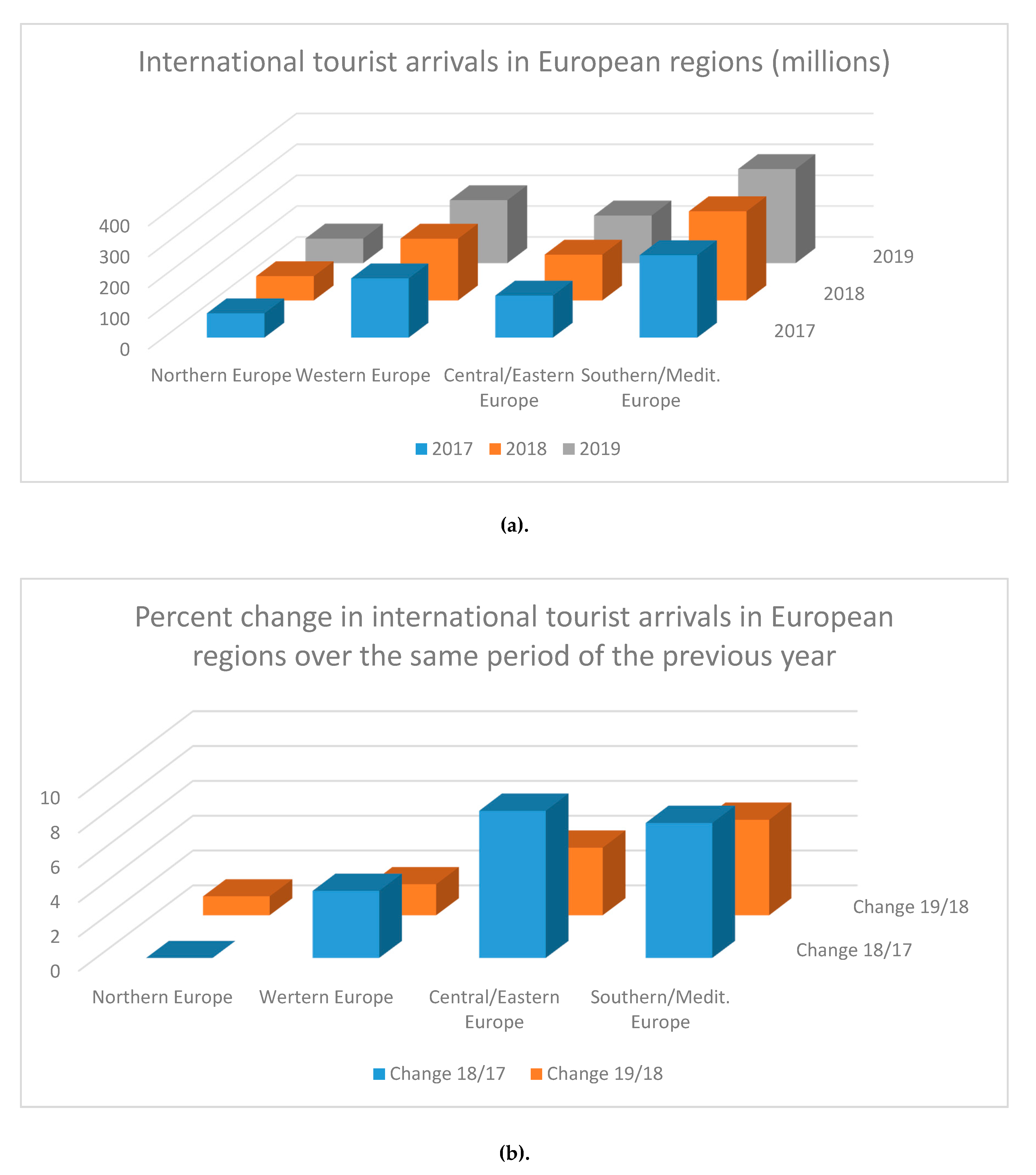
The 35 most competitive countries in tourism represent 84% of world tourism GDP and receive 70% of all international tourists [2,3]. For example, in the case of Europe, the European Travel Commission (2019) stated that most European countries increased the number of tourists (Figure 2). The European Travel Commission established a strong economic increase experienced by Europe in 2018 because GDP increased by 1.8% compared to the previous year. Much of the strong economic development was due to tourism, as the travel and tourism sector contributed directly to the Union’s gross domestic product (GDP) at a rate of 3.9% and accounted for 5.1% from the hand of total work in 2018.
As tourism grows, new opportunities for investment, development, and spending on infrastructure also arise, new income is generated, and living standards are increased [4]. Thus, it is widely accepted that international tourism promotes economic development, since it generates competitive advantages generating economic returns through specialization in the production of a tourist product [5]. Currently, one of the most significant debates in the field of economic growth is the measurement of the different effects of tourism development. Thus, great progress has now been established in the study of the relationships between both variables in numerous countries and regions [6,7,8]. To quantify the impact of the link established between these factors, in the last decade, numerous researchers have developed different statistical methods: The tourism satellite account (TSA), the computable general equilibrium (CGE), and dynamic stochastic general equilibrium (DSGE) models. TSA is the statistical technique that finds tourism as an industry and enables an adequate measuring of its input to the economy [9]. On the other hand, CGE quantifies the main economic changes, including those related to tourism, of the different industries [10]. However, both econometric techniques analyze the impact of tourism development on economic growth but do not determine a true cause–effect relationship [11]; further, they do so taking into account only a certain period. For this reason, researchers have sought other econometric techniques to verify whether tourism development has a significant effect on economic growth. To this end, DSGE was developed, which provides an empirical theoretical and structural explanation of macroeconomic relations and considers dynamic factors and stochastic terms under general equilibrium theory [12].
According to the World Tourism Organization and the International Monetary Fund, a slowdown in world economic growth is expected in 2020. For this reason, we intend to analyze whether an improvement in tourism productivity in some of the main tourist countries can prevent the slowdown in growth, which was experienced by, among others, the European GDP since 2018. Consequently, the objective of this research has been to try to demonstrate that the DSGE model can be applied to different tourist experiences and even increase the precision previously obtained by incorporating vector autoregression (VAR), building the well-known DSGE-VAR model. Using data from leading tourism countries such as France, Japan, and Germany, the impulse-response functions are also developed, including intervals to learn how an improvement in the productivity of the tourism sector can cause exogenous effects on economic growth, to help in a more precise way to the development and application of economic policies related to tourism development, something demanded by the previous literature [12,13,14].
More recently, the health crisis caused by the ‘COVID−19′ pandemic has paralyzed much of economic activity in a significant number of countries. One of the most affected sectors has been the tourism sector, which presumably will be one of the last sectors to resume its activity. These months of paralysis can seriously affect the viability of the sector, causing closure of companies and reduction of employment. This model can help articulate and simulate different and exceptional public policies for an extraordinary challenge such as the one that the tourism sector is experiencing. The results that this model can throw on this scenario can vary significantly since it will depend on the level of restrictions that have been applied in each country, both at a general level and at the level of the tourism sector. Those countries that apply a high level of restrictions will cause the level of investments to decrease and recover their level much more slowly than other sectors, considering the results obtained in this work. On the part of the productivity of the tourism sector, it will depend on the restrictions of both the sector and other sectors, since continued restrictions in non-tourism sectors may affect the dynamism observed in the production of tourism goods and services. These restrictions will also affect the added value of tourism goods and services but will have a high impact on other types of goods and services, since the sector has a high level of spillover towards other sectors. In short, the present model allows simulating the effects that the variation of a factor, such as investment or employment, may have on the other factors, both in the tourism sector and in the rest of the economy and its connections, in addition to evaluating possible policies by public institutions and other interest groups.
2. Literature Review
2.1. Background of Tourism Development
It is accepted that tourism development has a positive influence on the economy [15,16], leading to higher production, income, and employment, which promote growth and general economic development in a country [17]. Specifically, the existing empirical literature maintains that the number of tourists visiting a country is a fundamental factor for economic growth since tourism spending provides income to the destination country [18]. Likewise, these profits are used to promote the import of capital goods, which in turn will produce goods and services, which will imply the economic growth of the visiting country [19].
Although most of the studies carried out in this field tend to focus on issues such as job creation and multiplier effects, tourism has a dynamic effect on the economy through indirect effects and externalities in all economic sectors [20]. In this way, tourism stimulates investment in new infrastructure, produces economies of scale, and favors the spread of technical knowledge [18,21]. Similarly, tourism development also contributes to reducing poverty [22], because the promotion of unskilled jobs and the provision of part-time or seasonal jobs, manage to integrate people into employment through the long term [18]. Furthermore, the tourism industry also contributes to economic growth by increasing efficiency through competition between domestic companies and the destination of international tourists [18,23].
2.2. Tourism and Economic Growth.
Recently, a huge interest has arisen in establishing the relevance of tourism in economic growth, considering this measure to be fundamental for the development of tourism sector policies and, in turn, is useful as an evaluation to forecast visitor arrivals and benefits of tourism [24,25]. There is considerable prior research examining the different channels linking tourism to economic growth. In this way, numerous authors have established various variables that define these linking channels [8], such as structural breaks and exchange rates [26], remittances [27], information and communication technology [28], foreign direct investment [29], carbon emissions [30], trade openness [31], and energy consumption [32].
Empirical evidence has shown that there is a stable and durable connection between tourist progress and economic development [19]. This leads to a positive influence of tourist activity on economic development for various reasons [12]. The first of these is related to the increase in foreign currency since the entry of foreign currency into a country can be used to finance for foreign capital or primary goods employed in the production chain [33]. Secondly, we could consider the local investment, since tourism allows stimulating local investment in new infrastructures, such as the transportation facilities [34]. Thirdly, we could cite the labor force since tourism contributes to the generation of employment [35]. Lastly, we consider the diffusion of technical knowledge because tourism is an important diffusion factor of research and human capital accumulation [36]. But they can show differences between countries and considered periods [14].
Different econometric models have been applied to analyze the connection between tourist sector and economic development, for example TSA, CGE, and DSGE [14]. In these models, cointegration and Granger causality and cross-sectional data models are frequently used [24,37,38]. Other investigations have also measured this relationship through time series models [39,40]. However, some authors have used panel data models [13,41,42], because they provide greater efficiency in short-term predictions [43,44]. Although a large amount of empirical research has employed these econometric models, these techniques can analyze the steps between tourist progress and economic development [11]. For this reason, certain researchers have used other econometric techniques to check whether tourism development has a significant effect on economic growth.
TSA is a statistical technique that analyzes tourism as an industry and enables an adequate measuring of its input to the economy. This method is useful to ensure the homologation of data both between countries and another areas of sectors. TSA assesses the size of tourism and its input to GDP and employment in a period [9]. However, the TSA is only an econometric method that reports the significative contribution of tourism in a given time, generally on an annual data [45]. For this reason, the use of other methods is necessary to examine the total contribution of tourism [46,47].
CGE is used to estimate an economy’s reaction to changes in exogenous variables [14]. In this way, CGE quantifies the main economic changes, including those related to tourism, of the different industries [10]. They add an input–output basis but connect the sectors of economy, foreign exchange markets, spending behavior of consumers, and public institutions, and show the macro factors of the economy [48]. Thus, the evaluation of the indirect consequences of different industries on economic growth is possible [14].
Also, DSGE has managed to be a basic empirical method in macroeconomics [49]. However, the use of DSGE has been widely questioned in the literature, due to their inability to adjust the data [50]. Despite this, the fit of these models has been improving [12,51], so that later studies demonstrated a better empirical fit regardless of economic openness [52,53]. Wannapan, Chaiboonsri, and Sriboonchitta [54] applied DSGE for the experience in Thailand where it is evident that there are two tourist stages, the low season and the high season, with capital and work factors helping the economic expansion of the country in high season. Changes in trends conclude with the need to improve the design of public policies. Other recent studies have shown great results of precision and explanation with the use of DSGE models, evidencing the need for their generalization and a greater depth of estimation to get more information on the causality studied [14]. In contrast to the large amount of previous research used by TSA and CGE models, DSGE is seldom applied in tourism papers to analyze the connection framework of tourism development to economic growth [14]. Although some authors have used the DSGE approach in their research [49,55,56], Liu, Song, and Blake [13] were the first to introduce the first complete DSGE model in the tourism domain [13,14].
3. Method
According to Liu, Song, and Blake [13], a DSGE model can be used to examine tourism with the general balance of the economy (see Table 1 and Table 2). First of all, we have established a utility function of households as firms and households look forwards to get the maximum utility conditioned on budget and, as well, they seek to get profits depending on resource restrictions [14]. The agents are in complete information situation of the market, so households are not penalized to search for work, physical capital rental, land rental, and financial markets [14]. Secondly, we proposed the Cobb–Douglas form to estimate the production functions of the tourism and non-tourism activities [14]. Thirdly, we developed the productivity function connected to the effects of physical capital and public sector, in which we established the effects of public sector by the private sector, where zero denotes that there were no side effects [13]. Finally, we established a model to measure the export; for that purpose, we used the global price and income indices.
Against this backdrop, we developed a DSGE-VAR model. First, we determined a vector of endogenous variables to express the model VAR. Then, we defined the vector of VAR variables, where the trade-weighted nominal exchange rate in the United States was established. Therefore, a growth in the trade-weighted nominal exchange rate caused the U.S. dollar to depreciate. It is necessary to create stilted information in the DSGE model with regard the prior functions of the DSGE-VAR estimation. Then, this information was used for the prior distributions of VAR [14]. Finally, it was necessary to stipulate a posterior distribution: for the purpose of correctly estimate the model.
4. Model Estimation
4.1. Empirical Results
With the objective to estimate more reliable results in the simulation of the model, information used in this study was collected from the indicators with the sample period from 1992 Q1 to 2017 Q4 from Eurostat, for the cases of France and Germany, and e-Stat Statistics of Japan, for the Japanese case.
The factors represented were classified in different classes such as structural parameters, shock parameters, and steady-state values. The data of the prior distributions (or also called prior probabilities) of the parameters were extracted from [14,57] and official statistics. In this paper, we used the data for the parameters such as the depreciation rate of physical capital (δ) from [58]. The parameters in Ht and Ωi,t (i=T, NT) represent the accumulation of human capital and the spillover effects of physical capital [59,60], which address the spillover effects of capital about tourism sector. The data for the shock parameters were obtained from [61]. The choice of the prior distributions was defined by [13]. Steady-state data corresponding to the tourist industry were estimated using 2010−2017, and the steady-state data were estimated from official statistics of the countries used. Steady-state information is expressed in Table 3.
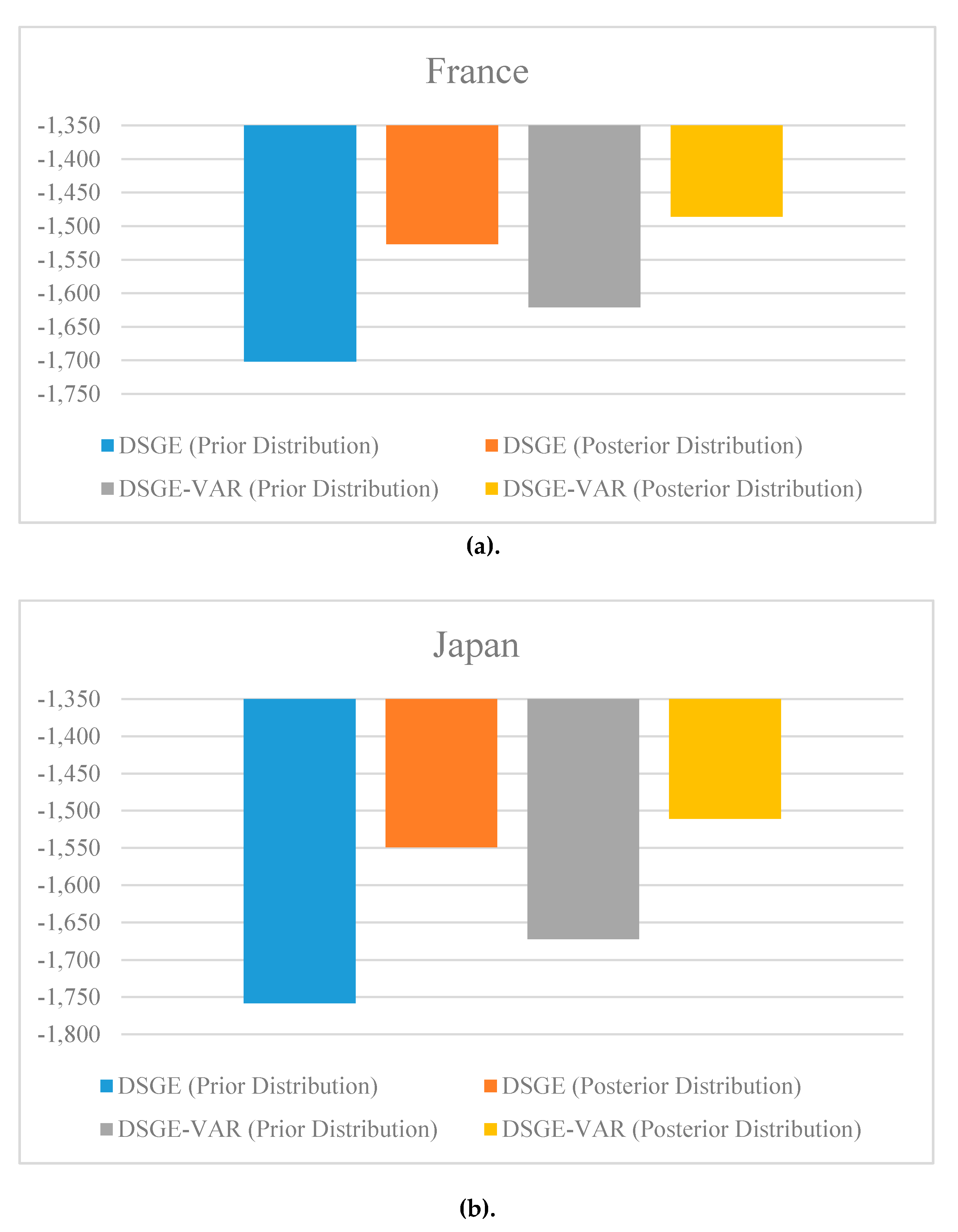
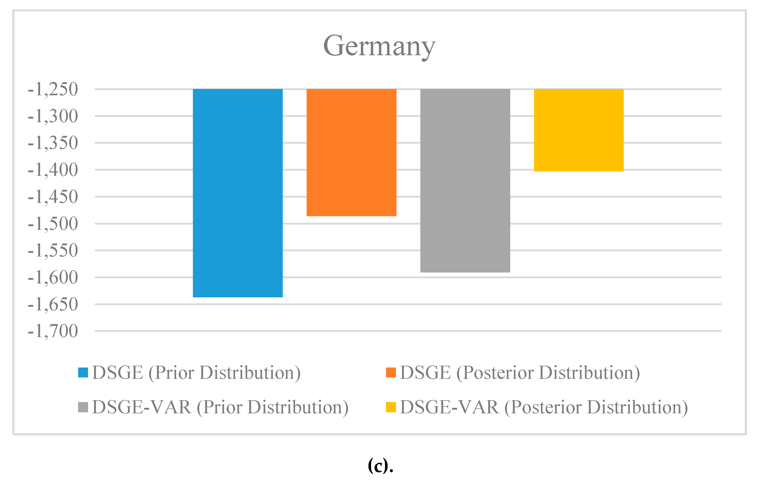
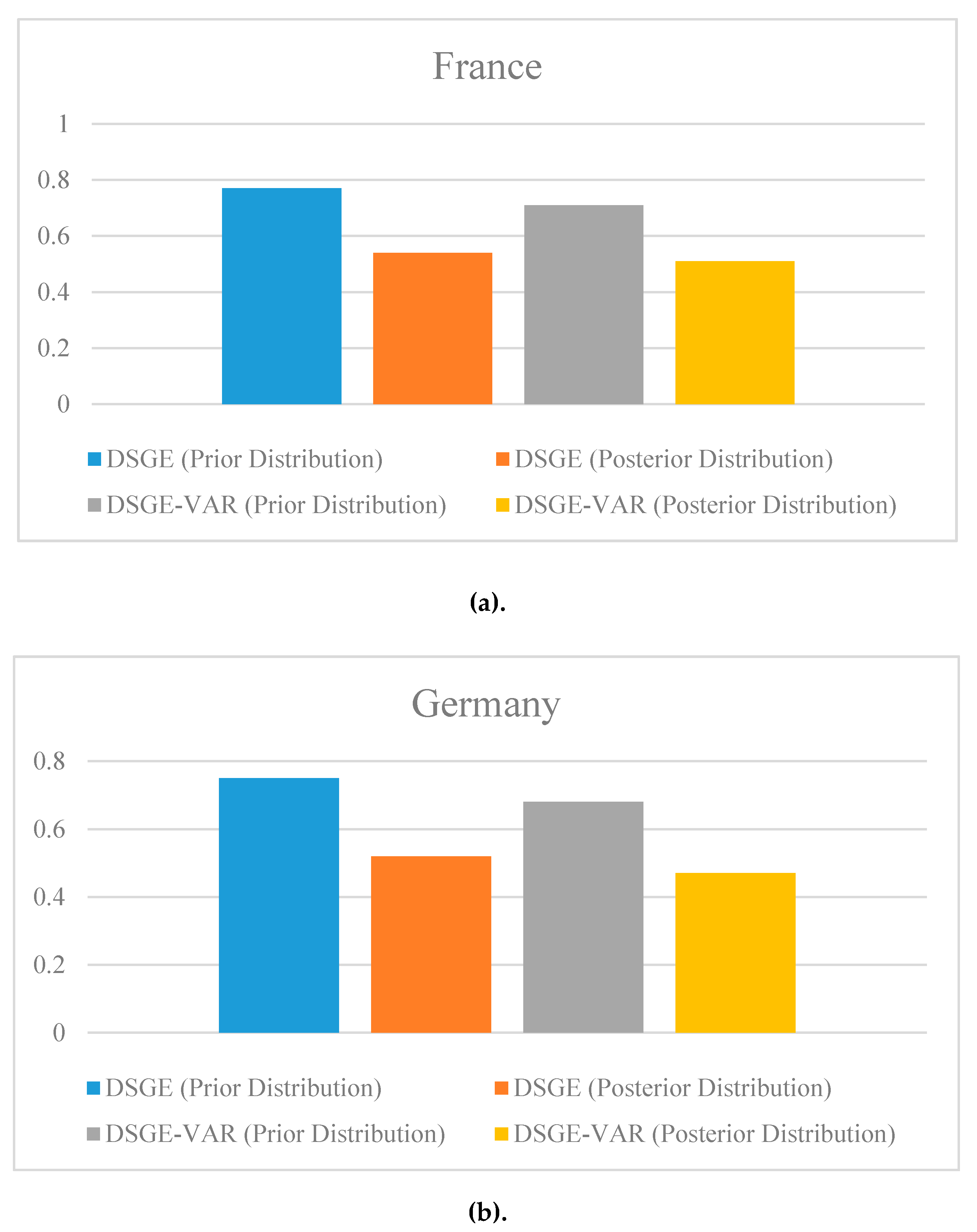
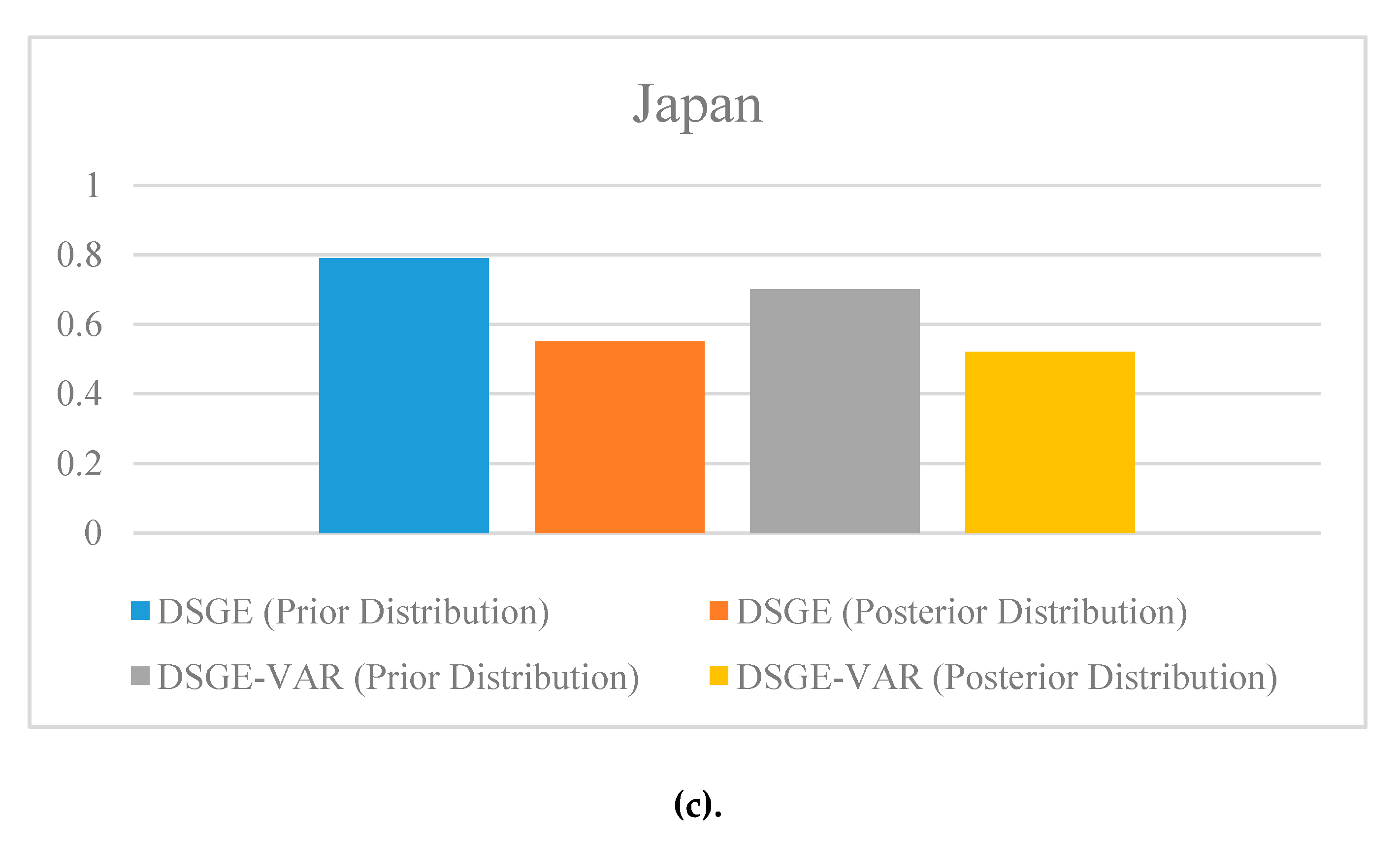
The present model is composed of 55 parameters. The Monte Carlo procedure was employed to calculate the posterior distributions (or also called posterior probabilities) and we used 20,000 simulations in every Markov sequence to compute the results of posterior distribution. Then, half of random simulations were eliminated. Also, to estimate the posterior probabilities, it usually computes for the DSGE models the marginal data density (MDD) p(Y) = ∫p(Y/θ) p(θ) dθ, because it supplies a summary on the accuracy of the results obtained by the model, representing a suitable criteria for the comparison of results and predictive capacity between models [43]. Figure 3 and Figure 4 show the mean and error (deviation) of MDD estimates after the computing of the DSGE and DSGE-VAR models created. Our results prove a high precision level shown by the DSGE-VAR model compared to DSGE for the three countries considered, if we observe the deviations obtained. These robustness results are within the normality shown by the DSGE-VAR models in previous studies [57].
Table 4, Table 5 and Table 6, point out the mean and standard deviation of the prior probabilities of every factor for France, Germany, and Japan, respectively. The mean of the posterior probabilities and the 90% confidence level estimated are reported. The estimation results of some of the structural parameters, such as β, δ, α3, α4, and h, work like the prior means following the same results of the previous literature [54]. The parameter α1 increased from 0.37 to 0.53 but α2 decreased from 0.44 to 0.07 for the French case. These changes were larger in the German case (α1 from 0.37 to 0.52 and α2 from 0.42 to 0.06) and in the case of Japan (α1 from 0.36 to 0.51, and α2 from 0.44 to 0.07). This means that the production of tourism products and services are safer in the cases of Germany and Japan against labor changes than the production of sectors other than the tourism sector.
On the other hand, the coefficients of leisure (ν1), private land (ν2), and intertemporal substitution (σ) were calculated as 1.93, 2.15, and 1.99 for the French case, which after dividing these results by unity, showed us elasticities of 0.52, 0.46, and 0.50, respectively. For the German case, these elasticities were 0.50, 0.48, and 0.52, for the mentioned variables, while for the Japanese model, these elasticities were 0.53, 0.47, and 0.52. In all cases, the elasticities were less than a 1, which is in line with previous works [13]. The substitute elasticity between tourist and non-tourist products (θ1) was 0.38, 0.40, and 0.35, for France, Germany, and Japan, respectively. These results of substitute elasticity were less than one, coinciding with the previous literature [62], and show a similar level of substitution of tourist products concerning non-tourist products and public services about changes in the price, with Japan being the most rigid case.
Regarding the coefficient of the elastic substitutional effect between FDI and domestic capital investment (θ2), we obtained a result of 1.45, 1.41, and 1.39, for France, Germany, and Japan, respectively. This coefficient shows that the higher the result, the greater the spill-over effect of FDI in the analyzed market. The results showed an acceptable level, but in the Japanese case, it showed a lower level than that obtained in other analyses [12,14,62]. In this case, the substitute elasticity between tourism and non-tourism imports is also not elastic (θ3), at 0.53, 0.57, and 0.59. They showed a similar level of substitution of tourism products concerning non-tourist products and public services concerning price changes, with Japan also being the most rigid case.
The price elasticity of tourism exports was modified, with a decrease from −0.39 to −0.38. The income elasticity of tourist exports incorporated important data, which led to a change from 0.81 in the prior distribution to 1.00 in the posterior distribution. According to the tourist statistics in the world [63], France, Germany, and Japan are among the most important tourist destinations. This means greater international incomes; more people visit these countries. Regarding non-tourism exports, the most valuable non-tourism goods from France, Germany, and Japan were vehicles, machinery, chemicals, and electronic elements. Nevertheless, these tourist products are not as competitive as tourism products. Hence, the price and income elasticities of the non-tourism sectors are much more rigid than the same elasticities of the tourist industry.
The most auto-regressive coefficients remained around 0.90, except for some variables such the productivity in the tourism industry (ρzt), the productivity in the public service (ρzp), and the land supply shock (ρLa). The coefficients of productivity in the tourism sector for France, Germany, and Japan were estimated as 0.53, 0.55, and 0.53, respectively. These results showed a lower level of productivity than other experiences analyzed, such as the Spanish one [13,14]. These levels of productivity may be linked to the strong hiring of temporary workers in the tourism sector, which causes a less than optimal level of human capital qualification compared to other sectors. The coefficient of productivity in the public service suffered the most abrupt decrease of the three countries analyzed since the coefficient in the prior distribution was estimated from 0.50 to 0.03 in the posterior distribution for France, from 0.52 to 0.05 for Germany, and from 0.51 to 0.07 from Japan, which shows low productivity of the public sector concerning the private sector, both with tourism and especially with non-tourism. Finally, for the coefficient of land supply shock, in the present study, we found highly developed countries, therefore the supply shocks of land were low since any new land entry available to the market is going to be easily acceptable, something similar to that shown by previous works [14,62].
4.2. Post-estimations
Impulse response functions (IRFs) were applied to describe the consequence of a tourism productivity shock on the economic growth in the countries analyzed. The shocks and confidence intervals of IRFs of selected variables used for periods 1, 5, and 10 in the models estimated are shown in Table 7.
For the French model, in the case of a 10% positive shock to the tourism sector productivity, the previous endowment of production variables remained, the supply of tourism services rose, and the price of tourism services fell by 14.34% (14.17% for the German model, and 15.94% for the Japanese model, with identical productivity shock). Regarding tourism exports, France showed an increase of 6.92% (6.05% for the German model, and 6.13% for the Japanese model). The tourist consumption benefited from this increase in productivity with a growth of 6.65%, 6.23%, and 6.59% in France, Germany, and Japan, respectively. With these results, it was confirmed that the price elasticity of tourist products was less than 1, within the parameters shown by the previous literature. By lowering prices, there was a greater consumption of this type of product, but the physical capital investment was reduced by 13.32%, 12.63%, and 11.85, respectively.
These results produced a boost of the value-added generated by the tourism industry by 4.73%, 4.82%, and 4.53% for France, Germany, and Japan, respectively. To continue with the successive increase in demand, households increase the level of investment in the tourism sector in years after the start of this productivity shock. In turn, this increase in investment produces an improvement in human capital, around 0.05% in the countries, which positively influences the rest of the sectors of the economy, such as the non-tourism sectors and the public sector. Continuing with the effects in the non-tourism sectors, productivity also increased, creating similar effects seen in the tourism sector. Non-tourism prices decreased in the three cases studied, where they decreased by around 1%, and non-tourism exports also increased slightly thanks to the drop in prices. However, in the case of consumption in non-tourism products, the results showed small decreases, of around 0.5%, due to greater dedication of household income to tourism consumption. As the demand for non-tourism products stagnated, it caused a small drop in investment in non-tourism sectors. Finally, thanks to the influence on the improvement of tourism productivity, the added value of non-tourism products also increased, albeit at a slower growth than that produced in tourism products (close to 0.3% for the group of countries analyzed). These results also showed differences with experiences analyzed by previous studies, where the consumption of non-tourism products grew after an increase in productivity in the tourism sector [12,13,14,15,16,17,18,19,20,21,22,23,24,25,26,27,28,29,30,31,32,33,34,35,36,37,38,39,40,41,42,43,44,45,46,47,48,49,50,51,52,53,54,55,56,57,58,59,60,61,62,63,64].
As for the GDP variable, this 10% increase in tourism productivity stimulated the GDP of France, Germany, and Japan by 0.53%, 0.56%, and 0.49%, respectively. The three countries analyzed have registered very moderate growth in recent years, following the trend of western countries. Therefore, as these are countries with a powerful tourism sector, any marginal increase in tourism productivity will significantly stimulate the GDP of these countries. These conclusions support the results shown by previous studies where there was a positive relationship between productivity and growth [12,62]. Our results increase the literature to give response on the spill-over shocks of physical and human capital and public sector on economic growth when an increase of productivity effects occurs [65]. Hence, the results obtained in this paper are an improvement for the tourism development literature and enhance the knowledge on the connection between tourist industry’ productivity and sustainable economic growth.
Finally, another important variable, unemployment, decreased by 4.76%, 4.82%, and 4.53% in France, Germany, and Japan, respectively. This was due to tourist employment increasing more than 1.5% in the countries analyzed, and also, the increase in tourist productivity benefited employment in the non-tourist sectors and the public sector, where it increased by around 0.6%. These results show higher unemployment reductions than those experienced by other countries, such as Spain, with an identical change in tourism productivity [14].
These results show how an increase in productivity in the tourism industry also produces a considerable increase in the consumption of tourism goods, but the influence that capital from the tourism sector has on the rest of the economy is more significant. Despite the abrupt drop that can originate in the investments of the tourist activity, the public institutions responsible for the politics in commerce and industry must stimulate the development of new techniques of production and management of the tourist companies like the automation and digital control of tourism services, or the shared value of such management with companies from other sectors, as this can maximize the added value created by the sector and its positive externalities in the rest of the economy. On the other hand, these possibilities of improving productivity and with it a further expansion of the tourism sector, create new opportunities for the creation of tourism employment, but also an improvement in human capital and employment in sectors not related to tourism activity.
5. Conclusion
This paper shows the generalization of the positive impact causes by tourism productivity in the economic growth and how these positive effects are spread in the improvement of non-tourism sectors and public goods, which is evidenced in the increase in added value and human capital more competitive. The model is calculated with a DSGE-VAR framework using quarterly data on France, Germany, and Japan from 1992 to 2017.
The estimation results show that an increase of 10% in tourism productivity can improve the value-added of the tourist industry overcomes around 3% and boosts around 0.5% of the GDP growth. Because we are dealing with the most important tourism countries in the world, any increase in tourism development will increase GDP in a considerable proportion. Likewise, the precision results show how the extended model of DSGE-VAR is better than the previous model of DSGE in the countries analyzed, both in estimating the prior and subsequent distribution. Also, while an increase in tourism productivity causes a fall in tourism prices, an increase in tourism consumption and, in principle, a fall in tourism investment, the positive effect in other sectors causes different consequences. An increase in non-tourism exports is observed, but a slight fall in the consumption of these non-tourism products and a longer fall in investment. These differences show different results from the previous experiences analyzed in tourism development [12,13,14]. Even so, this increase in tourism productivity leaves a spill-over in both capital and added value, as does employment in non-tourism sectors and the public sector.
This paper develops two important additions to the existing knowledge on tourism development. First, this paper expands the work of [13] by incorporating the VAR model into a DSGE framework for the model of tourism economics, and generalizing the model for any country. Second, this study analyzes how the factors of tourism performance stimulate tourist activity’ development and sustainable economic growth through the confidence intervals of the IRFs, which is a need demanded by the literature to offer policymakers the levels of response on the possible policies analyzed [12,14]. Finally, the relationships shown by the factors studied by our model and the behavior that it maintains over time helps governments and other policymakers to study different ways that obtain different positive externalities from the tourism sector towards other economic activities [13].
This work may also be a useful tool for managing the tourism sector in the face of the ‘COVID−19′ pandemic crisis. This model shows different possibilities of study regarding the initial situation of a parameter of said sector and how this parameter would affect the rest of the tourism sector as well as other economic sectors and the public sector. Furthermore, thanks to the calculation of the IRFs and their confidence intervals, it is possible to forecast the time durations of the effects caused by the change of a parameter and also how other parameters may evolve throughout a narrow range of results. Therefore, the reference of said time evolution of the parameters according to the tourism sector and other sectors can help control the effects that the public restrictions caused by the pandemic can produce and its trend according to the evolution of said restrictions.
The results of this study can envisage several future research ideas. In recent years, the effects of unconventional monetary policy have been increasingly analyzed. In this case, future research could focus on the effects of this kind of policy on the sustainability of economic growth, with indicators such as tourism expenditure and energy consumption. Likewise, another recent line of investigation of economic growth is the analysis of fiscal limits, so it would be convenient to study how the tourism sector would react to the application of different fiscal policies concerning other sectors. The introduction of tourist rentals as a new important market in the tourism sector and its effect on economic growth and tourism activity would be an interesting aspect to research.
Author Contributions
This study has been designed and performed by all of the authors. D.A. collected the data. D.A., A.L.-G., and J.R.S.-S. analyzed the data. The introduction and literature review were written by D.A. and A.L.-G. All of the authors wrote the discussion and conclusions. All authors have read and agreed to the published version of the manuscript.
Funding
This research was funded by the Universidad de Málaga and the APC was funded by the Universidad de Málaga.
Acknowledgments
The authors would like to express their sincere gratitude to the anonymous reviewers, and the editors for their truly valuable comments.
Conflicts of Interest
The authors declare no conflict of interest.
References
- UNWTO. World Tourism Barometer. In Proceedings of the Conference on Tourism and Accessibility, Madrid, Spain, 16–20 June 2019. [Google Scholar]
- World Economic Forum. The Travel & Tourism Competitiveness. In Travel and Tourism at a Tipping Point; World Economic Forum: Geneva, Switzerland, 2019. [Google Scholar]
- Notarstefano, C. European sustainable tourism: Context, concepts and guidelines for action. Int. J. Sustain. Econ. 2008, 1, 44. [Google Scholar] [CrossRef]
- Kruja, A. The Impact of Tourism Sector Development in the Albanian Economy. Econ. Seria Manag. 2012, 15, 204–218. [Google Scholar]
- Skerritt, D.; Huybers, T.; Lapatinas, A. The effect of the Internet on economic sophistication: An empirical analysis. Econ. Lett. 2019, 174, 35–38. [Google Scholar]
- Chatziantoniou, I.; Filis, G.; Eeckels, B.; Apostolakis, A. Oil prices, tourism income and economic growth: A structural VAR approach for European Mediterranean countries. Tour. Manag. 2013, 36, 331–341. [Google Scholar] [CrossRef] [Green Version]
- Van Der Marel, E. Economic effects of reform in professional services. Eur. Parliam. Int. Mark. Consum. Prot. 2017.
- Kumar, N.; Kumar, R.R.; Kumar, R.; Stauvermann, P.J. Is the tourism—Growth relationship asymmetric in the Cook Islands? Evidence from NARDL cointegration and causality tests. Tour. Econ 2019, 1–24. [Google Scholar] [CrossRef]
- Frechtling, D.C. Exploring the Full Economic Impact of Tourism for Policy Making: Extending the Use of the Tourism Satellite Account through Macroeconomic Analysis Tools. World Tour. Organ. 2011, 21. [Google Scholar]
- Dwyer, L.; Forsyth, P.; Spurr, R. Contrasting the Uses of TSAs and CGE Models: Measuring Tourism Yield and Productivity. Tour. Econ. 2007, 13, 537–551. [Google Scholar] [CrossRef]
- Song, H.; Dwyer, L.; Li, G.; Cao, Z. Tourism economics research: A review and assessment. Ann. Tour. Res. 2012, 39, 1653–1682. [Google Scholar] [CrossRef]
- Zhang, H.; Yang, Y. Prescribing for the tourism-induced Dutch disease: A DSGE analysis of subsidy policies. Tour. Econ. 2019, 25, 942–963. [Google Scholar] [CrossRef]
- Liu, A.; Song, H.; Blake, A. Modelling productivity shocks and economic growth using the Bayesian dynamic stochastic general equilibrium approach. Int. J. Contemp. Hosp. Manag. 2018, 30, 3229–3249. [Google Scholar] [CrossRef]
- Liu, A.; Wu, D.C. Tourism productivity and economic growth. Ann. Tour. Res. 2019, 76, 253–265. [Google Scholar] [CrossRef]
- Nizar, M.H. Pengaruh Pariwisata Terhadap Pertumbuhan Ekonomi Di Indonesia Tourism Effect on Economic Growth In Indonesia; University Library of Munich: Munich, Germany, 2011. [Google Scholar]
- Sugiyarto, G.; Blake, A.; Sinclair, M.T. Tourism and globalization: Economic Impact in Indonesia. Ann. Tour. Res. 2003, 30, 683–701. [Google Scholar] [CrossRef]
- Chingarande, A.; Saayman, A. Critical success factors for tourism-led growth. Int. J. Tour. Res. 2018, 20, 800–818. [Google Scholar] [CrossRef]
- Nyasha, S.; Odhiambo, N.M. Financial development and economic growth nexus: A rejoinder to Tsionas. Econ. Notes. 2019, 48, e12136. [Google Scholar] [CrossRef]
- Balaguer, J.; Cantavella-Jordá, M. Tourism as a long-run economic growth factor: The Spanish case. Appl. Econ. 2002, 34, 877–884. [Google Scholar] [CrossRef] [Green Version]
- Marin, D. Is the tourism-led growth thesis valid? The case of the bahamas, barbados, and Jamaica. Tour. Anal. 1992, 74, 678–688. [Google Scholar]
- Brida, J.G.; Sanchez Carrera, E.J.; Risso, W.A. Tourism’s impact on long-run Mexican economic growth. Econ. Bull. 2008, 3, 1–8. [Google Scholar]
- Ashley, C.; Mitchell, J. Can Tourism Reduce Poverty in Africa? Overseas Development Institute: London, UK, 2006. [Google Scholar]
- Bhagwati, J. International Factor Movements and National Advantage. Indian Econ. Soc. Hist. Rev. 1979, 14, 73–100. [Google Scholar]
- Pablo-Romero, M.P.; Molina, J.A. Tourism and economic growth: A review of empirical literature. Tour. Manag. Perspect. 2013, 8, 28–41. [Google Scholar] [CrossRef]
- Tang, C.F.; Tan, E.C. Does tourism effectively stimulate Malaysia’s economic growth? Tour. Manag. 2015, 46, 158–163. [Google Scholar] [CrossRef]
- Kumar, R.R.; Stauvermann, P.J.; Kumar, N.N.; Shahzad, S.J.H. Revisiting the threshold effect of remittances on total factor productivity growth in South Asia: A study of Bangladesh and India. Appl. Econ. 2018, 50, 2860–2877. [Google Scholar] [CrossRef]
- Kumar, R.R. Exploring the nexus between tourism, remittances and growth in Kenya. Qual. Quant. 2014, 48, 1573–1588. [Google Scholar] [CrossRef]
- Kumar, R.R.; Kumar, R. Exploring the nexus between information and communications technology, tourism and growth in Fiji. Tour. Econ. 2012, 18, 359–371. [Google Scholar] [CrossRef]
- Khoshnevis, Y.S.; Salehi, H.K.; Soheilzad, M. The relationship between tourism, foreign direct investment and economic growth: Evidence from Iran. Curr. Issues Tour. 2017, 20, 15–26. [Google Scholar] [CrossRef]
- Lee, J.W.; Brahmasrene, T. Investigating the influence of tourism on economic growth and carbon emissions: Evidence from panel analysis of the European Union. Tour. Manag. 2013, 38, 69–76. [Google Scholar] [CrossRef]
- Shahbaz, M.; Kumar, R.R.; Ivanov, S.; Loganathan, N. The nexus between tourism demand and output per capita with the relative importance of trade openness and financial development: A study of Malaysia. Tour. Econ. 2017, 23, 168–186. [Google Scholar] [CrossRef] [Green Version]
- Isik, C.; Dogru, T.; Turk, E.S. A nexus of linear and non-linear relationships between tourism demand, renewable energy consumption, and economic growth: Theory and evidence. Int. J. Tour. Res. 2018, 20, 38–49. [Google Scholar] [CrossRef]
- Nowak, J.J.; Sahli, M.; Cortés-Jiménez, I. x Tourism, capital good imports and economic growth: Theory and evidence for Spain. Tour. Econ. 2007, 13, 515–536. [Google Scholar] [CrossRef]
- Chou, M.C. Does tourism development promote economic growth in transition countries? A panel data analysis. Econ. Model. 2013, 33, 226–232. [Google Scholar] [CrossRef] [Green Version]
- Inchausti-Sintes, F. Tourism: Economic growth, employment and Dutch Disease. Ann. Tour. Res. 2015, 54, 172–189. [Google Scholar] [CrossRef]
- Sihabutr, C. Technology and International Specialisation in Tourism. Ph.D. Thesis, Université Toulouse le Mirail, Toulouse, France, 2012. [Google Scholar]
- Brida, J.G.; Cortes-Jimenez, I.; Pulina, M. Has the tourism-led growth hypothesis been validated? A literature review. Curr. Issues Tour. 2016, 19, 394–430. [Google Scholar] [CrossRef]
- Chiu, Y.B.; Yeh, L.T. The Threshold Effects of the Tourism-Led Growth Hypothesis: Evidence from a Cross-sectional Model. J. Travel Res. 2017, 56, 625–637. [Google Scholar] [CrossRef]
- Belloumi, M. The relationship between tourism receipts, real effective exchange rate and economic growth in Tunisia. Int. J. Tour. Res. 2010, 12, 550–560. [Google Scholar] [CrossRef]
- Shahzad, S.J.H.; Shahbaz, M.; Ferrer, R.; Kumar, R.R. Tourism-led growth hypothesis in the top ten tourist destinations: New evidence using the quantile-on-quantile approach. Tour. Manag. 2017, 60, 223–232. [Google Scholar] [CrossRef] [Green Version]
- Bilen, M.; Yilanci, V.; Eryüzlü, H. Tourism development and economic growth: A panel Granger causality analysis in the frequency domain. Curr. Issues Tour. 2017, 20, 27–32. [Google Scholar] [CrossRef]
- Salifou, C.K.; ul Haq, I. Tourism, globalization and economic growth: A panel cointegration analysis for selected West African States. Curr. Issues Tour. 2017, 20, 664–667. [Google Scholar] [CrossRef]
- Wu, D.C.; Song, H.; Shen, S. New developments in tourism and hotel demand modeling and forecasting. Int. J. Contemp. Hosp. Manag. 2017, 29, 507–529. [Google Scholar] [CrossRef]
- Song, H.; Qiu, R.T.R.; Park, J. A review of research on tourism demand forecasting. Ann. Tour. Res. 2019, 75, 338–362. [Google Scholar] [CrossRef]
- Frenţ, C. Informing tourism policy with statistical data: The case of the Icelandic Tourism Satellite Account. Curr. Issues Tour. 2018, 21, 1033–1051. [Google Scholar] [CrossRef]
- Giannopoulos, K.; Boutsinas, B. Tourism Satellite Account Support Using Online Analytical Processing. J. Travel Res. 2016, 55, 95–112. [Google Scholar] [CrossRef]
- Wu, Y.H.; Ho, C.C.; Lin, E.S. Measuring the Impact of Military Spending: How Far Does a DSGE Model Deviate from Reality? Def. Peace Econ. 2017, 28, 585–608. [Google Scholar] [CrossRef]
- Blake, A.; Sinclair, M.T. La gestion de crise pour le tourisme: La réponse des Etats-Unis au 11 septembre. Ann. Tour. Res. 2003, 30, 813–832. [Google Scholar] [CrossRef]
- Smets, F.; Wouters, R. An estimated dynamic stochastic general equilibrium model of the euro area. J. Eur. Econ. Assoc. 2003, 1, 1123–1175. [Google Scholar] [CrossRef] [Green Version]
- Pagan, A. Report on modelling and forecasting at the Bank of England / Bank’s response to the Pagan report. Bank Engl. Q. Bull. 2003, 43, 60–91. [Google Scholar]
- Christiano, L.J.; Eichenbaum, M.; Evans, C.L. Nominal Rigidities and the Dynamic Effects of a Shock to Monetary Policy. J. Polit. Econ. 2005, 113, 1–45. [Google Scholar] [CrossRef] [Green Version]
- Smets, F.; Wouters, R. Forecasting with a Bayesian DSGE model: An application to the euro area. JCMS J. Common Mark. Stud. 2004, 42, 841–867. [Google Scholar] [CrossRef] [Green Version]
- Adolfson, M.; Lindé, J.; Villani, M. Forecasting Performance of an Open Economy DSGE Model. Economet. Rev. 2007, 26, 289–328. [Google Scholar] [CrossRef]
- Wannapan, S.; Chaiboonsri, C.; Sriboonchitta, S. Application of the Bayesian DSGE model to the international tourism sector: Evidence from Thailand’s economic cycle. Wit. Trans. Ecol. Envir. 2018, 227, 257–268. [Google Scholar]
- Rouwenhorst, K.G. Time to build and aggregate fluctuations. A reconsideration. J. Monet. Econ. 1991, 27, 241–254. [Google Scholar] [CrossRef]
- Hazari, B.R.; Sgro, P.M. Tourism and growth in a dynamic model of trade. J. Int. Trade Econ. Dev. 1995, 4, 243–252. [Google Scholar]
- Herbst, E.W.; Schorfheide, F. Bayesian Estimation of DSGE Models; Princeton University Press: Princeton, NJ, USA, 2015. [Google Scholar]
- Burriel, P.; Fernández-Villaverde, J.; Rubio-Ramírez, J.F. MEDEA: A DSGE model for the Spanish economy. SERIE 2010, 1, 175–243. [Google Scholar] [CrossRef]
- Zhang, J. Assessing the Economic Importance of Meetings Activities in Denmark. Scand. J. Hosp. Tour. 2014, 14, 192–210. [Google Scholar] [CrossRef]
- Zhang, W.B. Tourism, trade externalities and public goods in a three-sector growth model. UTMS J. Econ. 2015, 6, 1–19. [Google Scholar]
- Gertler, M.; Sala, L.; Trigari, A. An Estimated Monetary DSGE Model with Unemployment and Staggered Nominal Wage Bargaining. J. Money Credit Bank 2008, 40, 1713–1764. [Google Scholar] [CrossRef]
- Tsionas, E.G.; Assaf, A. Short-run and long-run performance of international tourism: Evidence from Bayesian dynamic models. Tour. Manag. 2014, 42, 22–36. [Google Scholar] [CrossRef]
- UNWTO. Report on Tourism and Culture Synergies. In Proceedings of the International Conference on Tourism and Accessibility, Madrid, Spain, 16–20 June 2018. [Google Scholar]
- Wu, D.C.; Liu, J.; Song, H.; Liu, A.; Fu, H. Developing a Web-based regional tourism satellite account (TSA) information system. Tour. Econ. 2019, 25, 67–84. [Google Scholar] [CrossRef]
- Mankiw, N.G.; Romer, D.; Weil, D.N. A Contribution to the Empirics of Economic Growth. Q. J. Econ. 1992, 107, 407–437. [Google Scholar] [CrossRef]
Figure 1.
(a). International tourism (Tourist arrivals in millions); (b). International tourism (Change in tourist arrivals in percentage for the previous year); (c). International tourism (Change in tourist arrivals in percentage for the last quarter of previous year).
Figure 1.
(a). International tourism (Tourist arrivals in millions); (b). International tourism (Change in tourist arrivals in percentage for the previous year); (c). International tourism (Change in tourist arrivals in percentage for the last quarter of previous year).

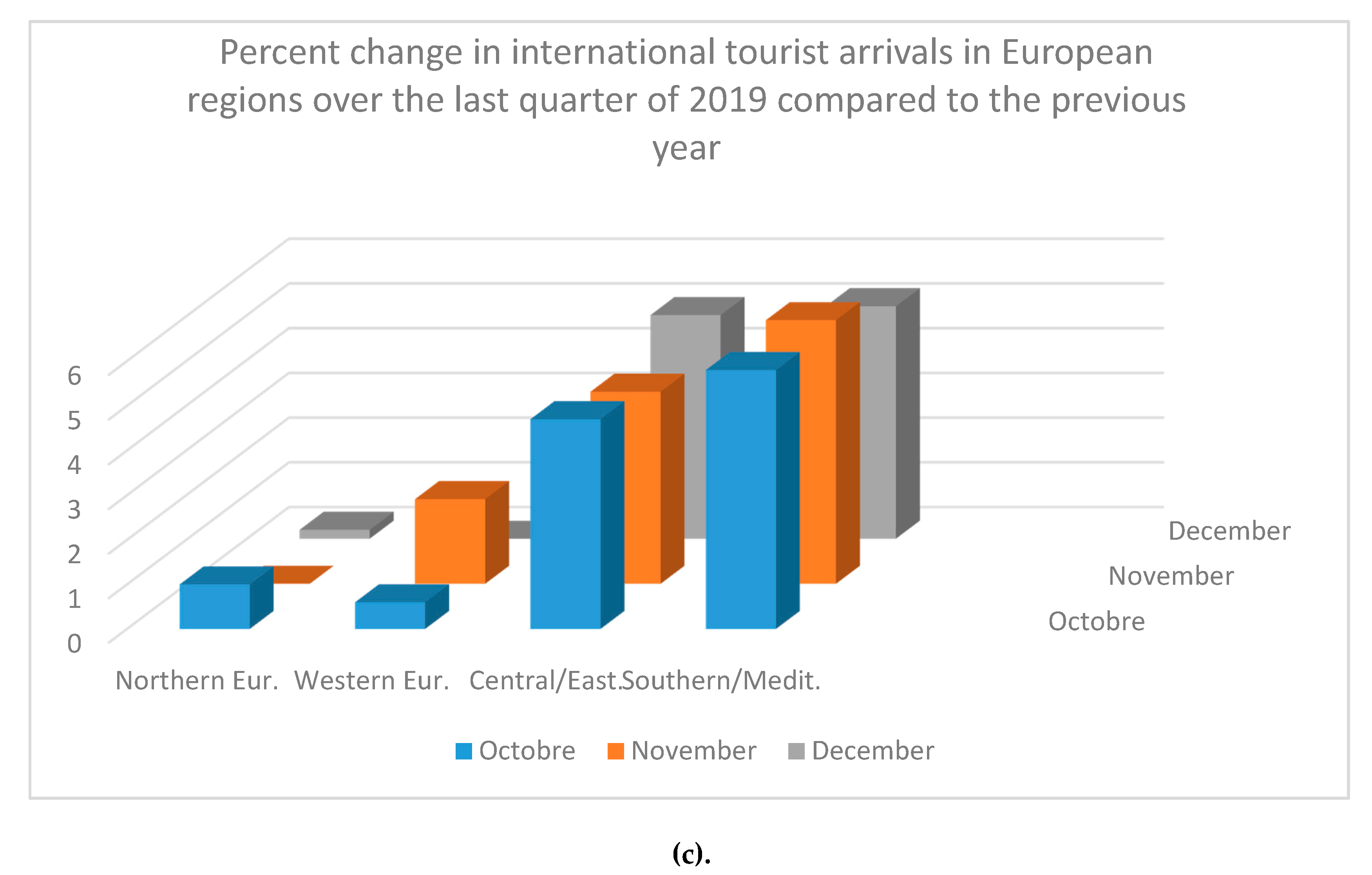
Figure 2.
(a). European tourism (Change in tourist arrivals in percentage for the previous year); (b). European tourism (Tourist arrivals in millions); (c). European tourism (Change in tourist arrivals in percentage for the last quarter of previous year).
Figure 2.
(a). European tourism (Change in tourist arrivals in percentage for the previous year); (b). European tourism (Tourist arrivals in millions); (c). European tourism (Change in tourist arrivals in percentage for the last quarter of previous year).


Figure 3.
(a). Mean (log marginal data density (MDD)); (b). Mean (log marginal data density (MDD)); (c). Mean (log marginal data density (MDD))
Figure 3.
(a). Mean (log marginal data density (MDD)); (b). Mean (log marginal data density (MDD)); (c). Mean (log marginal data density (MDD))


Figure 4.
(a). Standard deviation (log MDD); (b). Standard deviation (log MDD); (c). Standard deviation (log MDD).
Figure 4.
(a). Standard deviation (log MDD); (b). Standard deviation (log MDD); (c). Standard deviation (log MDD).


Table 1.
Dynamic stochastic general equilibrium (DSGE).
| Functions | Variables |
|---|---|
| The utility function of households | |
| E0: expected utility function β: discounted rate h: typifies the habit persistence of consumption Ct: (using a CES function) is composed by:
Lal,t: Private land supply shock Ϛla,t: This exogenous variable represents the result of private land inputs on the economy σ, ν1, and ν2: the parameters of the constant elasticity of substitution (CES) CM, t: is composed by:
| |
| The production functions of the tourism and non-tourism activities | |
| Yi,t (i = T, NT): The value-added of the given sector Ωi, t (i = T, NT): The productivity function connected to the effects of physical capital and public sector Ki,t (i = T, NT): The physical capital and is calculated by the process: Ki, t+1 = Ii, t + (1−δ)Ki, t (i= T, NT)
| |
| The productivity function connected to the effects of physical capital and public sector | |
| At: The auto-regression processes of the total productivity shocks Ai,t: The auto-regression processes of the sector that point out sector and total productivity shocks ζP, t: The exogenous shock to the spill-over effects of public sector YP,t the effect of public sector Ki,t: The effect of physical capital : The spillover effect of Kp,t φP,i: The effect of the public sector φc,i:The effect of the private sector (i = T, NT): The parameters | |
| The spill-over effects of capital and the accumulation of human capital | |
| EXT,t: The exports of tourism ζH,t: The shock to human capital accumulation EXNT,t: The non-tourism products and : The effect of the tourism product on human capital ai, bi and πi: The parameters δH: The depreciation rate of human capital : The externality of experience | |
| The exports | |
| The real exchange rate in USD RERt: The exchange rate YROW,t: The world income level | |
Table 2.
DSGE-vector autoregression (VAR) model.
| Functions | Variables |
|---|---|
| The model VAR | |
| : represent an nH × 1 vector corresponding to endogenous variables for t = 1…, T c: Group of terms p: The VAR lag length [B1, …, Bp]: Parameter matrices ut: The vector of forecast errors defined by the multivariate normal distribution N (0; ∑u) | |
| Vector of VAR variables | |
| YT,t: The production in the tourist industry YNT,t: The production in the non- tourist industries Ct: Per capita real consumption GDPt: Per capita real GDP Pt: Applies the GDP deflator Rt: The federal funds rate adjusted at the annual rate EXt: The trade-weighted nominal exchange rate in the United | |
| The DSGE-VAR estimation | |
| be a T×nH matrix with each row consisting of Xv be a T×k matrix with the t-th row containing in where k ≡ 1 + p× nH. ϕ: The maximum-likelihood estimator is calculated according to DSGE parameters vector | |
| DSGE parameters vector | |
| θ: Vector consisting of the DSGE parameters EDh: The expectation operator conditional on the DSGE parameter vector θ | |
Table 3.
Steady-state data.
| Variables | Code | Value in Steady State | Time Period |
|---|---|---|---|
| GDP/GDP | Y | 1.00 | – |
| Tourism Value Added/GDP | YT | 0.11 | 2002–2017 |
| Non-tourism Value Added/GDP | YNT | 0.72 | 2002–2017 |
| Public Service Value Added/GDP | YP | 0.17 | 2002–2017 |
| Final Consumption/GDP | C | 0.58 | 2002–2017 |
| Total Investment/GDP | Ī | 0.21 | 2002–2017 |
| Imports/GDP | CM | 0.29 | 2002–2017 |
| Tourism Exports/GDP | EXNT | 0.05 | 2002–2017 |
| Non-tourism Exports/GDP | EXT | 0.23 | 2002–2017 |
| Tourism Imports/GDP | CMT | 0.01 | 2002–2017 |
| Non-tourism Imports/GDP | CMNT | 0.29 | 2002–2017 |
| Tourism Investment/GDP | IT | 0.01 | 2002–2017 |
| Non-tourism Investment/GDP | INT | 0.16 | 2002–2017 |
| Public Service Investment/GDP | IP | 0.04 | 2002–2017 |
| Tourism FDI/GDP | ĪT DF | 0.01 | 2002–2017 |
| Non-tourism FDI/GDP | ĪNTDF | 0.06 | 2002–2017 |
| Balance of Payments/GDP | BP | 0.04 | 2002–2017 |
| Unemployment | u | 0.15 | 2002–2017 |
| Tourism Consumption/(Final Consumption + Imports) | γ1 | 0.08 | 2002–2017 |
| Non-tourism Consumption/(Final Consumption + Imports) | γ2 | 0.50 | 2002–2017 |
| Public Service Consumption/(Final Consumption + Imports) | γ3 | 0.20 | 2002–2017 |
| Tourism Employment/Employment | nT | 0.11 | 2002–2016 |
| Non-tourism Employment/Employment | nNT | 0.59 | 2002–2017 |
| Public Service Employment/Employment | nP | 0.27 | 2002–2017 |
| CPI | P | 1.00 | – |
| Tourism Price | PT | 1.00 | – |
| Non-tourism Price | PNT | 1.00 | – |
| Public Good Price | PP | - | - |
| GDP Growth Rate | gy | Log (1.02) | 1992–2017 |
| Final Consumption Growth Rate | gC | Log (1.02) | 1992–2017 |
| Investment Growth Rate | gI | Log (1.02) | 1992–2017 |
| Government Consumption Growth Rate | gP | Log (1.02) | 1992–2017 |
| Exports Growth Rate | gEX | Log (1.03) | 1992–2017 |
| Production Tax Rate | τY | 0.12 | – |
Note: Real terms of the GDP index (2010 = 100).
Table 4.
Estimation results for France.
| Prior Distribution | Posterior Distribution | 90% Interval | |||||
|---|---|---|---|---|---|---|---|
| Low | High | ||||||
| Structure Parameter | β | Beta (0.99,0.00) | 0.99 | 0.99 | 0.99 | ||
| Discount Rate | |||||||
| Physical Capital Depreciation Rate | δ | Beta (0.02,0.00) | 0.02 | 0.02 | 0.02 | ||
| Output Elasticity of Physical Capital in the Tourism Industry | α1 | Beta (0.37,0.10) | 0.53 | 0.51 | 0.60 | ||
| Output Elasticity of Human Capital in the Tourism Industry | α2 | Beta (0.44,0.10) | 0.07 | 0.03 | 0.11 | ||
| Output Elasticity of Physical Capital in the Non-tourism Industry | α3 | Beta (0.63,0.10) | 0.65 | 0.60 | 0.70 | ||
| Output Elasticity of Physical Capital in the Public Service Industry | α4 | Beta (0.63,0.10) | 0.69 | 0.65 | 0.73 | ||
| Habit Persistent | h | Beta (0.85,0.01) | 0.85 | 0.85 | 0.86 | ||
| Elasticity of Leisure | ν1 | Gamma (2.00,0.10) | 1.98 | 1.93 | 2.09 | ||
| Elasticity of Private Land | ν2 | Gamma (2.00,0.10) | 2.10 | 2.02 | 2.18 | ||
| Elasticity of Intertemporal Substitution | σ | Gamma (2.00,0.10) | 1.94 | 1.91 | 1.98 | ||
| Substitute Elasticity between Tourism, Non-tourism Goods and Public Services | θ1 | Gamma (0.40,0.10) | 0.38 | 0.37 | 0.40 | ||
| Substitute Elasticity between FDI and Domestic Investment | θ2 | Gamma (1.51,0.10) | 1.45 | 1.41 | 1.47 | ||
| Substitute Elasticity between Tourism and Non-tourism Imports | θ3 | Gamma (0.40,0.10) | 0.53 | 0.51 | 0.56 | ||
| Price Elasticity of Tourism Exports (Absolute) | θEX,T | Gamma (0.39,0.10) | 0.38 | 0.35 | 0.41 | ||
| Price Elasticity of Non-tourism Exports (Absolute) | θE, | NT | Gamma (0.19,0.10) | 0.32 | 0.28 | 0.35 | |
| Income Elasticity of Tourism Exports | ωT | Gamma (0.81,0.10) | 1.00 | 0.94 | 1.12 | ||
| Income Elasticity of Non-tourism Exports | ωNT | Gamma (0.27,0.10) | 0.05 | 0.03 | 0.07 | ||
| Autoregressive Coefficient of Return Rate | θtr | Beta (0.80,0.10) | 0.95 | 0.92 | 0.96 | ||
| Elasticity of Price in the Taylor Rule | θp | Gamma (1.70,0.10) | 1.73 | 1.69 | 1.76 | ||
| Elasticity of GDP in the Taylor Rule | θy | Gamma (0.12,0.05) | 0.13 | 0.13 | 0.14 | ||
| Elasticity of Tourism Exports in Human Capital Accumulation | aT | Gamma (0.30,0.10) | 0.48 | 0.43 | 0.51 | ||
| Elasticity of Non-exports of the Tourism Industry in Human Capital Accumulation | bT | Gamma (0.05,0.01) | 0.04 | 0.04 | 0.05 | ||
| Scale Effect of Human Capital Accumulated by the Tourism Industry | πT | Gamma (0.30,0.10) | 0.31 | 0.28 | 0.33 | ||
| Elasticity of Non-tourism Exports in Human Capital Accumulation | a T | Gamma (0.30,0.10) | 0.43 | 0.39 | 0.46 | ||
| Elasticity of Non-exports in the Non-tourism industry of Human Capital Accumulation | B T | Gamma (0.06,0.01) | 0.06 | 0.05 | 0.06 | ||
| Scale Effect of Human Capital Accumulated by the Non-tourism Industry | Π T | Gamma (0.30,0.10) | 0.38 | 0.34 | 0.41 | ||
| Depreciation Rate of Human Capital | δH | Gamma (0.04,0.01) | 0.05 | 0.04 | 0.05 | ||
| Spill-over Effect of Public Service on Tourism Productivity | φP, | T | Gamma (0.10,0.01) | 0.10 | 0.10 | 0.11 | |
| Spill-over Effect of Tourism Physical Capital on its Productivity | φT | Gamma (0.05,0.01) | 0.05 | 0.05 | 0.06 | ||
| Congestion Effect of Physical Capital on Tourism Productivity | φC, | T | Gamma (0.04,0.01) | 0.04 | 0.04 | 0.05 | |
| Spill-over Effect of Public Service on Non-tourism Productivity | φP, | NT | Gamma (0.10,0.01) | 0.11 | 0.11 | 0.11 | |
| Spill-over Effect of Non-tourism Physical Capital on its Productivity | φ T | Gamma (0.05,0.01) | 0.04 | 0.04 | 0.05 | ||
| Congestion Effect of Physical Capital on Non-tourism Productivity | φC, | NT | Gamma (0.05,0.01) | 0.04 | 0.04 | 0.05 | |
| Autoregressive Parameter | |||||||
| Productivity of the Tourism Industry | Ρ T | Beta (0.50,0.20) | 0.53 | 0.47 | 0.68 | ||
| Productivity of the Non-Tourism Industry | ρZNNT | Beta (0.50,0.20) | 0.99 | 0.99 | 0.10 | ||
| Productivity of the Public Service Industry | ρZ P | Beta (0.50,0.20) | 0.03 | 0.02 | 0.04 | ||
| Total Productivity of all Industries | ρZ | Beta (0.51,0.20) | 0.91 | 0.90 | 0.93 | ||
| World Output | ρYrow | Beta (0.50,0.20) | 0.92 | 0.91 | 0.94 | ||
| Real Exchange Rate | ρRER | Beta (0.78,0.20) | 0.84 | 0.83 | 0.84 | ||
| Land Supply Shock | ρLa | Beta (0.50,0.20) | 0.30 | 0.16 | 0.38 | ||
| Tourism Imports Price | ρC, | T | Beta (0.51,0.20) | 0.85 | 0.78 | 0.90 | |
| Non-tourism Imports | ρC, | NT | Beta (0.50,0.20) | 0.86 | 0.84 | 0.86 | |
| Human Capital Accumulation Shock | ρH | Beta (0.50,0.20) | 0.82 | 0.74 | 0.94 | ||
| Public Service Production Shock | ρP | Beta (0.50,0.20) | 0.10 | 0.99 | 1.00 | ||
| Standard Deviation | εZT | IGamma (0.15, 0.25) | 0.13 | 0.11 | 0.15 | ||
| Productivity of the Tourism Industry | |||||||
| Productivity of the Non-Tourism Industry | εZNT | IGamma (0.15, 0.25) | 0.13 | 0.12 | 0.14 | ||
| Productivity of the Public Service Industry | εZP | IGamma (0.15, 0.25) | 0.14 | 0.11 | 0.16 | ||
| Total Productivity of all Industries | εZ | IGamma (0.15, 0.25) | 0.10 | 0.10 | 0.10 | ||
| World Output | εYrow | IGamma (0.15, 0.25) | 0.11 | 0.10 | 0.12 | ||
| Real Exchange Rate | εRER | IGamma (0.15, 0.25) | 0.11 | 0.10 | 0.11 | ||
| Land Supply Shock | εLa | IGamma (0.15, 0.25) | 0.36 | 0.31 | 0.42 | ||
| Tourism Imports Price | εCM, | T | IGamma (0.15, 0.25) | 0.20 | 0.14 | 0.29 | |
| Non-tourism Imports | εCM, | NT | IGamma (0.15, 0.25) | 0.50 | 0.45 | 0.52 | |
| Human Capital Accumulation Shock | εH | IGamma (0.15, 0.25) | 0.13 | 0.11 | 0.14 | ||
| Public Service Production Shock | εP | IGamma (0.15, 0.25) | 0.25 | 0.22 | 0.27 | ||
Table 5.
Estimation results for Germany.
| Prior Distribution | Posterior Distribution | 90% Interval | |||||
|---|---|---|---|---|---|---|---|
| Low | High | ||||||
| Structure Parameter Discount Rate | β | Beta (0.95, 0.00) | 0.95 | 0.95 | 0.95 | ||
| Physical Capital Depreciation Rate | δ | Beta (0.02,0.00) | 0.02 | 0.02 | 0.03 | ||
| Output Elasticity of Physical Capital in the Tourism Industry | α1 | Beta (0.37,0.10) | 0.52 | 0.50 | 0.58 | ||
| Output Elasticity of Human Capital in the Tourism Industry | α2 | Beta (0.42,0.10) | 0.06 | 0.03 | 0.09 | ||
| Output Elasticity of Physical Capital in the Non-tourism Industry | α3 | Beta (0.63,0.10) | 0.60 | 0.57 | 0.66 | ||
| Output Elasticity of Physical Capital in the Public Service Industry | α4 | Beta (0.63,0.10) | 0.65 | 0.62 | 0.71 | ||
| Habit Persistent | h | Beta (0.85,0.01) | 0.88 | 0.87 | 0.88 | ||
| Elasticity of Leisure | ν1 | Gamma (2.00,0.10) | 1.93 | 1.90 | 1.97 | ||
| Elasticity of Private Land | ν2 | Gamma (2.00,0.10) | 2.15 | 2.13 | 2.19 | ||
| Elasticity of Intertemporal Substitution | σ | Gamma (2.00,0.10) | 1.99 | 1.94 | 2.12 | ||
| Substitute Elasticity between Tourism, Non-tourism Goods and Public Services | θ1 | Gamma (0.40,0.10) | 0.40 | 0.38 | 0.41 | ||
| Substitute Elasticity between FDI and Domestic Investment | θ2 | Gamma (1.51,0.10) | 1.41 | 1.38 | 1.45 | ||
| Substitute Elasticity between Tourism and Non-tourism Imports | θ3 | Gamma (0.40,0.10) | 0.57 | 0.52 | 0.59 | ||
| Price Elasticity of Tourism Exports (Absolute) | θEX,T | Gamma (0.39,0.10) | 0.34 | 0.32 | 0.41 | ||
| Price Elasticity of Non-tourism Exports (Absolute) | θE, | NT | Gamma (0.20,0.10) | 0.30 | 0.28 | 0.33 | |
| Income Elasticity of Tourism Exports | ωT | Gamma (0.82,0.10) | 1.05 | 0.97 | 1.11 | ||
| Income Elasticity of Non-tourism Exports | ωNT | Gamma (0.27,0.10) | 0.06 | 0.05 | 0.08 | ||
| Autoregressive Coefficient of Return Rate | θtr | Beta (0.80,0.10) | 0.93 | 0.90 | 0.95 | ||
| Elasticity of Price in the Taylor Rule | θp | Gamma (1.71,0.10) | 1.70 | 1.68 | 1.74 | ||
| Elasticity of GDP in the Taylor Rule | θy | Gamma (0.13,0.05) | 0.13 | 0.12 | 0.13 | ||
| Elasticity of Tourism Exports in Human Capital Accumulation | aT | Gamma (0.30,0.10) | 0.49 | 0.44 | 0.52 | ||
| Elasticity of Non-exports of the Tourism Industry in Human Capital Accumulation | bT | Gamma (0.06,0.01) | 0.06 | 0.06 | 0.07 | ||
| Scale Effect of Human Capital Accumulated by the Tourism Industry | πT | Gamma (0.30,0.10) | 0.36 | 0.33 | 0.38 | ||
| Elasticity of Non-tourism Exports in Human Capital Accumulation | a T | Gamma (0.30,0.10) | 0.47 | 0.43 | 0.48 | ||
| Elasticity of Non-exports in the Non-tourism industry of Human Capital Accumulation | b T | Gamma (0.05,0.01) | 0.08 | 0.07 | 0.08 | ||
| Scale Effect of Human Capital Accumulated by the Non-tourism Industry | Π T | Gamma (0.30,0.10) | 0.40 | 0.36 | 0.42 | ||
| Depreciation Rate of Human Capital | δH | Gamma (0.05,0.01) | 0.07 | 0.06 | 0.07 | ||
| Spill-over Effect of Public Service on Tourism Productivity | φP, | T | Gamma (0.10,0.01) | 0.13 | 0.12 | 0.13 | |
| Spill-over Effect of Tourism Physical Capital on its Productivity | φT | Gamma (0.05,0.01) | 0.07 | 0.06 | 0.09 | ||
| Congestion Effect of Physical Capital on Tourism Productivity | φC, | T | Gamma (0.04,0.01) | 0.06 | 0.05 | 0.06 | |
| Spill-over Effect of Public Service on Non-tourism Productivity | φP, | NT | Gamma (0.10,0.01) | 0.13 | 0.13 | 0.15 | |
| Spill-over Effect of Non-tourism Physical Capital on its Productivity | Φ T | Gamma (0.05,0.01) | 0.03 | 0.03 | 0.04 | ||
| Congestion Effect of Physical Capital on Non-tourism Productivity | φC, | NT | Gamma (0.05,0.01) | 0.05 | 0.05 | 0.06 | |
| Autoregressive Parameter | |||||||
| Productivity of the Tourism Industry | Ρ T | Beta (0.50,0.20) | 0.55 | 0.48 | 0.70 | ||
| Productivity of the Non-Tourism Industry | ρZ T | Beta (0.50,0.20) | 0.93 | 0.92 | 0.93 | ||
| Productivity of the Public Service Industry | ρ P | Beta (0.52,0.20) | 0.05 | 0.04 | 0.07 | ||
| Total Productivity of all Industries | ρZ | Beta (0.51,0.20) | 0.97 | 0.93 | 0.90 | ||
| World Output | ρYrow | Beta (0.53,0.20) | 0.98 | 0.94 | 0.99 | ||
| Real Exchange Rate | ρRER | Beta (0.78,0.20) | 0.84 | 0.83 | 0.84 | ||
| Land Supply Shock | ρLa | Beta (0.52,0.20) | 0.31 | 0.21 | 0.37 | ||
| Tourism Imports Price | ρCM, | T | Beta (0.51,0.20) | 0.87 | 0.82 | 0.90 | |
| Non-tourism Imports | ρCM, | NT | Beta (0.50,0.20) | 0.82 | 0.80 | 0.85 | |
| Human Capital Accumulation Shock | ρH | Beta (0.53,0.20) | 0.87 | 0.79 | 0.93 | ||
| Public Service Production Shock | ρP | Beta (0.50,0.20) | 0.99 | 0.98 | 1.00 | ||
| Standard Deviation | εZT | IGamma (0.15, 0.25) | 0.12 | 0.10 | 0.14 | ||
| Productivity of the Tourism Industry | |||||||
| Productivity of the Non-Tourism Industry | εZNT | IGamma (0.15, 0.25) | 0.15 | 0.14 | 0.16 | ||
| Productivity of the Public Service Industry | εZP | IGamma (0.15, 0.25) | 0.14 | 0.13 | 0.16 | ||
| Total Productivity of all Industries | εZ | IGamma (0.15, 0.25) | 0.13 | 0.12 | 0.15 | ||
| World Output | εYrow | IGamma (0.15, 0.25) | 0.13 | 0.11 | 0.16 | ||
| Real Exchange Rate | εRER | IGamma (0.15, 0.25) | 0.12 | 0.11 | 0.12 | ||
| Land Supply Shock | εLa | IGamma (0.15, 0.25) | 0.34 | 0.31 | 0.40 | ||
| Tourism Imports Price | εCM, | T | IGamma (0.15, 0.25) | 0.18 | 0.14 | 0.28 | |
| Non-tourism Imports | εCM, | NT | IGamma (0.15, 0.25) | 0.48 | 0.45 | 0.51 | |
| Human Capital Accumulation Shock | εH | IGamma (0.15, 0.25) | 0.14 | 0.13 | 0.15 | ||
| Public Service Production Shock | εP | IGamma (0.15, 0.25) | 0.24 | 0.21 | 0.27 | ||
Table 6.
Estimation results for Japan.
| Low | High | ||||||
|---|---|---|---|---|---|---|---|
| Structure Parameter Discount Rate | β | Beta (0.95, 0.00) | 0.95 | 0.95 | 0.95 | ||
| Physical Capital Depreciation Rate | δ | Beta (0.02,0.00) | 0.02 | 0.02 | 0.03 | ||
| Output Elasticity of Physical Capital in the Tourism Industry | α1 | Beta (0.37,0.10) | 0.52 | 0.50 | 0.58 | ||
| Output Elasticity of Human Capital in the Tourism Industry | α2 | Beta (0.42,0.10) | 0.06 | 0.03 | 0.09 | ||
| Output Elasticity of Physical Capital in the Non-tourism Industry | α3 | Beta (0.63,0.10) | 0.60 | 0.57 | 0.66 | ||
| Output Elasticity of Physical Capital in the Public Service Industry | α4 | Beta (0.63,0.10) | 0.65 | 0.62 | 0.71 | ||
| Habit Persistent | h | Beta (0.85,0.01) | 0.88 | 0.87 | 0.88 | ||
| Elasticity of Leisure | ν1 | Gamma (2.00,0.10) | 1.93 | 1.90 | 1.97 | ||
| Elasticity of Private Land | ν2 | Gamma (2.00,0.10) | 2.15 | 2.13 | 2.19 | ||
| Elasticity of Intertemporal Substitution | σ | Gamma (2.00,0.10) | 1.99 | 1.94 | 2.12 | ||
| Substitute Elasticity between Tourism, Non-tourism Goods and Public Services | θ1 | Gamma (0.40,0.10) | 0.40 | 0.38 | 0.41 | ||
| Substitute Elasticity between FDI and Domestic Investment | θ2 | Gamma (1.51,0.10) | 1.41 | 1.38 | 1.45 | ||
| Substitute Elasticity between Tourism and Non-tourism Imports | θ3 | Gamma (0.40,0.10) | 0.57 | 0.52 | 0.59 | ||
| Price Elasticity of Tourism Exports (Absolute) | θEX,T | Gamma (0.39,0.10) | 0.34 | 0.32 | 0.41 | ||
| Price Elasticity of Non-tourism Exports (Absolute) | θE, | NT | Gamma (0.20,0.10) | 0.30 | 0.28 | 0.33 | |
| Income Elasticity of Tourism Exports | ωT | Gamma (0.82,0.10) | 1.05 | 0.97 | 1.11 | ||
| Income Elasticity of Non-tourism Exports | ωNT | Gamma (0.27,0.10) | 0.06 | 0.05 | 0.08 | ||
| Autoregressive Coefficient of Return Rate | θtr | Beta (0.80,0.10) | 0.93 | 0.90 | 0.95 | ||
| Elasticity of Price in the Taylor Rule | θp | Gamma (1.71,0.10) | 1.70 | 1.68 | 1.74 | ||
| Elasticity of GDP in the Taylor Rule | θy | Gamma (0.13,0.05) | 0.13 | 0.12 | 0.13 | ||
| Elasticity of Tourism Exports in Human Capital Accumulation | aT | Gamma (0.30,0.10) | 0.49 | 0.44 | 0.52 | ||
| Elasticity of Non-exports of the Tourism Industry in Human Capital Accumulation | bT | Gamma (0.06,0.01) | 0.06 | 0.06 | 0.07 | ||
| Scale Effect of Human Capital Accumulated by the Tourism Industry | πT | Gamma (0.30,0.10) | 0.36 | 0.33 | 0.38 | ||
| Elasticity of Non-tourism Exports in Human Capital Accumulation | a T | Gamma (0.30,0.10) | 0.47 | 0.43 | 0.48 | ||
| Elasticity of Non-exports in the Non-tourism industry of Human Capital Accumulation | b T | Gamma (0.05,0.01) | 0.08 | 0.07 | 0.08 | ||
| Scale Effect of Human Capital Accumulated by the Non-tourism Industry | Π T | Gamma (0.30,0.10) | 0.40 | 0.36 | 0.42 | ||
| Depreciation Rate of Human Capital | δH | Gamma (0.05,0.01) | 0.07 | 0.06 | 0.07 | ||
| Spill-over Effect of Public Service on Tourism Productivity | φP, | T | Gamma (0.10,0.01) | 0.13 | 0.12 | 0.13 | |
| Spill-over Effect of Tourism Physical Capital on its Productivity | φT | Gamma (0.05,0.01) | 0.07 | 0.06 | 0.09 | ||
| Congestion Effect of Physical Capital on Tourism Productivity | φC, | T | Gamma (0.04,0.01) | 0.06 | 0.05 | 0.06 | |
| Spill-over Effect of Public Service on Non-tourism Productivity | φP, | NT | Gamma (0.10,0.01) | 0.13 | 0.13 | 0.15 | |
| Spill-over Effect of Non-tourism Physical Capital on its Productivity | Φ T | Gamma (0.05,0.01) | 0.03 | 0.03 | 0.04 | ||
| Congestion Effect of Physical Capital on Non-tourism Productivity | φC, | NT | Gamma (0.05,0.01) | 0.05 | 0.05 | 0.06 | |
| Autoregressive Parameter | |||||||
| Productivity of the Tourism Industry | Ρ T | Beta (0.50,0.20) | 0.55 | 0.48 | 0.70 | ||
| Productivity of the Non-Tourism Industry | ρZ T | Beta (0.50,0.20) | 0.93 | 0.92 | 0.93 | ||
| Productivity of the Public Service Industry | ρ P | Beta (0.52,0.20) | 0.05 | 0.04 | 0.07 | ||
| Total Productivity of all Industries | ρZ | Beta (0.51,0.20) | 0.97 | 0.93 | 0.90 | ||
| World Output | ρYrow | Beta (0.53,0.20) | 0.98 | 0.94 | 0.99 | ||
| Real Exchange Rate | ρRER | Beta (0.78,0.20) | 0.84 | 0.83 | 0.84 | ||
| Land Supply Shock | ρLa | Beta (0.52,0.20) | 0.31 | 0.21 | 0.37 | ||
| Tourism Imports Price | ρCM, | T | Beta (0.51,0.20) | 0.87 | 0.82 | 0.90 | |
| Non-tourism Imports | ρCM, | NT | Beta (0.50,0.20) | 0.82 | 0.80 | 0.85 | |
| Human Capital Accumulation Shock | ρH | Beta (0.53,0.20) | 0.87 | 0.79 | 0.93 | ||
| Public Service Production Shock | ρP | Beta (0.50,0.20) | 0.99 | 0.98 | 1.00 | ||
| Standard Deviation | εZT | IGamma (0.15, 0.25) | 0.12 | 0.10 | 0.14 | ||
| Productivity of the Tourism Industry | |||||||
| Productivity of the Non-Tourism Industry | εZNT | IGamma (0.15, 0.25) | 0.15 | 0.14 | 0.16 | ||
| Productivity of the Public Service Industry | εZP | IGamma (0.15, 0.25) | 0.14 | 0.13 | 0.16 | ||
| Total Productivity of all Industries | εZ | IGamma (0.15, 0.25) | 0.13 | 0.12 | 0.15 | ||
| World Output | εYrow | IGamma (0.15, 0.25) | 0.13 | 0.11 | 0.16 | ||
| Real Exchange Rate | εRER | IGamma (0.15, 0.25) | 0.12 | 0.11 | 0.12 | ||
| Land Supply Shock | εLa | IGamma (0.15, 0.25) | 0.34 | 0.31 | 0.40 | ||
| Tourism Imports Price | εCM, | T | IGamma (0.15, 0.25) | 0.18 | 0.14 | 0.28 | |
| Non-tourism Imports | εCM, | NT | IGamma (0.15, 0.25) | 0.48 | 0.45 | 0.51 | |
| Human Capital Accumulation Shock | εH | IGamma (0.15, 0.25) | 0.14 | 0.13 | 0.15 | ||
| Public Service Production Shock | εP | IGamma (0.15, 0.25) | 0.24 | 0.21 | 0.27 | ||
Table 7.
Impulse response functions with confidence intervals.
| France | Germany | Japan | |||||
|---|---|---|---|---|---|---|---|
| Variables | Period | Shock | 90% C. I. | Shock | 90% C. I. | Shock | 90% C. I. |
| Tourism Productivity | 1 | 10.00 | [9.37, 10.00] | 10.00 | [9.30, 10.00] | 10.00 | [8.85, 10.00] |
| 5 | 2.62 | [1.75, 3.26] | 2.55 | [1.67, 3.14] | 2.32 | [1.59, 3.04] | |
| 10 | 0.58 | [0.11, 0.85] | 0.43 | [0.08, 0.74] | 0.40 | [0.08, 0.68] | |
| Tourism Price | 1 | −14.34 | [−12.65, −16.07] | −14.18 | [−12.25, −15.73] | −15.94 | [−12.79, −16.37] |
| 5 | −2.44 | [−1.58, −3.62] | −2.17 | [−1.33, −3.16] | −2.28 | [−1.41, −3.37] | |
| 10 | −0.67 | [0.00, −1,45] | −0.51 | [0.00, −1,23] | −0.53 | [0.01, −1,36] | |
| Tourism Exports | 1 | 6.93 | [6.15, 7.67] | 6.05 | [5.63, 6.86] | 6.47 | [5.881 7.56] |
| 5 | 1.57 | [0.79, 2.82] | 1.36 | [0.64, 2.48] | 1.48 | [0.73, 2.55] | |
| 10 | 0.48 | [0.06, 0.75] | 0.38 | [0.03, 0.72] | 0.34 | [0.02, 0.67] | |
| Tourism Consumption | 1 | 6.66 | [5.86, 7.25] | 6.23 | [5.53, 7.04] | 6.59 | [5.87, 7.23] |
| 5 | 1.42 | [0.63, 2.57] | 1.55 | [0.70, 2.63] | 1.72 | [0.83, 2.82] | |
| 10 | 0.52 | [0.14, 0.86] | 0.62 | [0.17, 0.91] | 0.75 | [0.23, 0.99] | |
| Tourism Investments | 1 | −13.33 | [−15.47, −12.35] | −12.63 | [−14.89, −11.33] | −11.86 | [−13.68, −11.42] |
| 5 | 2.84 | [−1.35, 4.63] | 2.45 | [−1.78, 4.51] | 2.17 | [−2.57, 4.02] | |
| 10 | 0.35 | [−2.04, 2.47] | 0.51 | [−2.38, 2.83] | 0.41 | [−2.15, 2.17] | |
| Tourism Value Added | 1 | 4.74 | [3.76, 6.15] | 4.04 | [3.23, 5.75] | 4.84 | [3.67, 6.43] |
| 5 | 0.55 | [0.23, 1.52] | 0.37 | [0.10, 1.12] | 0.58 | [0.31, 1.32] | |
| 10 | 0.36 | [−0.18, 0.82] | 0.29 | [−0.21, 0.78] | 0.49 | [−0.12, 0.95] | |
| Human Capital | 1 | 0.05 | [0.04, 0.07] | 0.06 | [0.05, 0.07] | 0.05 | [0.04, 0.07] |
| 5 | 0.02 | [0.01, 0.04] | 0.03 | [0.02, 0.05] | 0.03 | [0.02, 0.04] | |
| 10 | 0.01 | [−0.02, 0.02] | 0.02 | [−0.01, 0.03] | 0.02 | [−0.01, 0.04] | |
| Tourism Capital Spill-over | 1 | 10.88 | [8.53, 11.95] | 10.46 | [8.42, 11.43] | 10.16 | [8.24, 11.28] |
| 5 | 2.33 | [1.36, 3.28] | 2.18 | [1.24, 3.18] | 2.18 | [1.17, 3.24] | |
| 10 | 0.65 | [0.03, 1.06] | 0.54 | [−0.16, 0.82] | 0.58 | [−0.12, 0.85] | |
| Non-tourism Price | 1 | −0.96 | [−1.38, −0.46] | −0.99 | [−1.40, −0.49] | −0.91 | [−1.31, −0.46] |
| 5 | −0.15 | [−0.52, 0.33] | −0.16 | [−0.52, 0.38] | −0.13 | [−0.51, 0.43] | |
| 10 | −0.04 | [−0.24, 0.47] | −0.03 | [−0.21, 0.49] | −0.07 | [−0.21, 0.49] | |
| Non-tourism Exports | 1 | 0.34 | [0.20, 0.48] | 0.32 | [0.17, 0.44] | 0.36 | [0.23, 0.49] |
| 5 | 0.06 | [−0.13, 0.25] | 0.04 | [−0.15, 0.23] | 0.08 | [0.20, 0.48] | |
| 10 | 0.02 | [−0.17, 0.18] | 0.01 | [−0.17, 0.18] | 0.02 | [−0.15, 0.19] | |
| Non-tourism Consumption | 1 | −0.47 | [−0.67, −0.23] | −0.52 | [−0.61, −0.28] | −0.49 | [−0.59, −0.24] |
| 5 | −0.15 | [−0.33, −0.02] | −0.13 | [−0.30, −0.04] | −0.18 | [−0.39, −0.05] | |
| 10 | −0.07 | [−0.20, 0.15] | −0.06 | [−0.16, 0.18] | −0.08 | [−0.17, 0.19] | |
| Non-tourism Investments | 1 | −0.69 | [−0.93, −0.49] | −0.77 | [−0.97, −0.51] | −0.61 | [−0.96, −0.51] |
| 5 | −0.16 | [−0.35, −0.13] | −0.08 | [−0.32, −0.10] | −0.10 | [−0.35, −0.13] | |
| 10 | 0.03 | [−0.15, 0.18] | 0.01 | [−0.17, 0.16] | −0.02 | [−0.18, 0.12] | |
| Non-tourism Value Added | 1 | 0.25 | [0.43, 0.13] | 0.29 | [0.47, 0.14] | 0.29 | [0.48, 0.16] |
| 5 | 0.05 | [−0.18, 0.18] | 0.05 | [−0.20, 0.21] | 0.05 | [−0.19, 0.22] | |
| 10 | 0.08 | [−0.21, 0.23] | 0.06 | [−0.17, 0.24] | 0.07 | [−0.16, 0.26] | |
| Non-tourism Capital Spill-over | 1 | 0.58 | [0.27, 0.72] | 0.53 | [0.24, 0.68] | 0.58 | [0.24, 0.70] |
| 5 | 0.13 | [−0.05, 0.28] | 0.09 | [−0.14, 0.19] | 0.12 | [−0.11, 0.21] | |
| 10 | 0.04 | [−0.17, 0.20] | 0.03 | [−0.14, 0.16] | 0.04 | [−0.14, 0.18] | |
| Public Goods Sector Value Added | 1 | 0.16 | [0.04, 0.33] | 0.12 | [−0.04, 0.32] | 0.13 | [−0.02, 0.34] |
| 5 | −0.17 | [−0.33, 0.08] | −0.09 | [−0.26, 0.12] | −0.14 | [−0.31, 0.09] | |
| 10 | −0.07 | [−0.17, 0.15] | −0.04 | [−0.15, 0.19] | −0.05 | [−0.15, 0.19] | |
| GDP | 1 | 0.54 | [0.47, 0,68] | 0.56 | [0.52, 0,61] | 0.49 | [0.40, 0,52] |
| 5 | 0.28 | [−0.13, 0.34] | 0.23 | [−0.15, 0.32] | 0.30 | [−0.09, 0.34] | |
| 10 | 0.07 | [−0.17, 0.18] | 0.05 | [−0.18, 0.16] | 0.04 | [−0.19, 0.16] | |
| Tourism Employment | 1 | 1.73 | [2.00, 1.53] | 1.85 | [2.13, 1.58] | 1.63 | [1.88, 1.52] |
| 5 | 0.62 | [0.44, 0.78] | 0.67 | [0.46, 0.80] | 0.43 | [0.46, 0.80] | |
| 10 | 0.05 | [−0.11, 0.16] | 0.06 | [−0.11, 0.16] | 0.04 | [−0.11, 0.16] | |
| Non-tourism Employment | 1 | 0.65 | [0.57, 0.82] | 0.73 | [0.58, 0.89] | 0.70 | [0.59, 0.87] |
| 5 | 0.14 | [−0.09, 0.26] | 0.17 | [−0.07, 0.28] | 0.15 | [−0.06, 0.25] | |
| 10 | 0.03 | [−0.13, 0.18] | 0.02 | [−0.13, 0.13] | 0.03 | [−0.10, 0.13] | |
| Public Goods Sector Employment | 1 | 0.68 | [0.58, 0.79] | 0.57 | [0.47, 0.66] | 0.59 | [0.48, 0.68] |
| 5 | 0.06 | [−0.11, 0.14] | 0.04 | [−0.09, 0.14] | 0.04 | [−0.07, 0.12] | |
| 10 | 0.03 | [−0.08, 0.15] | −0.01 | [−0.10, 0.10] | 0.02 | [−0.05, 0.11] | |
| Unemployment | 1 | −4.76 | [−5.05, −4.33] | −4.82 | [−5.22, −4.40] | −4.53 | [−4.79, −4.38] |
| 5 | −1.05 | [−1.43, −0.77] | −0.93 | [−1.32, −0.70] | −0.90 | [−1.22, −0.71] | |
| 10 | −0.02 | [−0.13, 0.14] | −0.03 | [−0.11, 0.10] | −0.02 | [−0.10, 0.09] | |
Note: 90% C.I.
© 2020 by the authors. Licensee MDPI, Basel, Switzerland. This article is an open access article distributed under the terms and conditions of the Creative Commons Attribution (CC BY) license (http://creativecommons.org/licenses/by/4.0/).
Share and Cite
MDPI and ACS Style
Alaminos, D.; León-Gómez, A.; Sánchez-Serrano, J.R. A DSGE-VAR Analysis for Tourism Development and Sustainable Economic Growth. Sustainability 2020, 12, 3635. https://0-doi-org.brum.beds.ac.uk/10.3390/su12093635
AMA Style
Alaminos D, León-Gómez A, Sánchez-Serrano JR. A DSGE-VAR Analysis for Tourism Development and Sustainable Economic Growth. Sustainability. 2020; 12(9):3635. https://0-doi-org.brum.beds.ac.uk/10.3390/su12093635
Chicago/Turabian StyleAlaminos, David, Ana León-Gómez, and José Ramón Sánchez-Serrano. 2020. "A DSGE-VAR Analysis for Tourism Development and Sustainable Economic Growth" Sustainability 12, no. 9: 3635. https://0-doi-org.brum.beds.ac.uk/10.3390/su12093635
Note that from the first issue of 2016, this journal uses article numbers instead of page numbers. See further details here.