High-Resolution Electricity Spot Price Forecast for the Danish Power Market

Abstract

Energy markets with a high penetration of renewables are more likely to be challenged by price variations or volatility, which is partly due to the stochastic nature of renewable energy. The Danish electricity market (DK1) is a great example of such a market, as 49% of the power production in DK1 is based on wind power, conclusively challenging the electricity spot price forecast for the Danish power market. The energy industry and academia have tried to find the best practices for spot price forecasting in Denmark, by introducing everything from linear models to sophisticated machine-learning approaches. This paper presents a linear model for price forecasting—based on electricity consumption, thermal power production, wind production and previous electricity prices—to estimate long-term electricity prices in electricity markets with a high wind penetration levels, to help utilities and asset owners to develop risk management strategies and for asset valuation.

1. Introduction

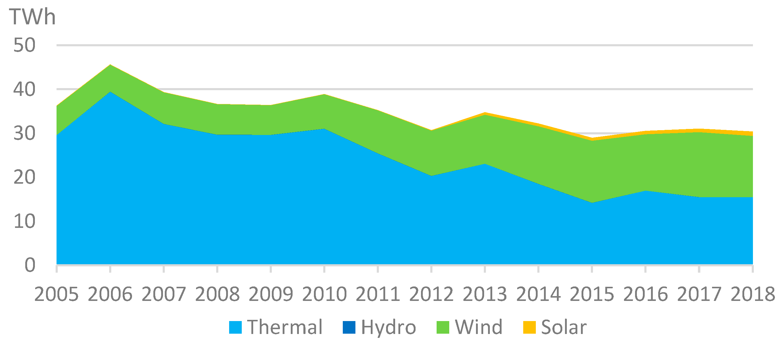
The installed capacity of wind power has increased in the Danish power market over the past 10–15 years, resulting in an increasing share of renewable power production in the Danish power market [1]. In 2005, renewable power production accounted for roughly 18% of the total power production in Denmark, and increased to more than 47% of the total power production in late 2019. The development of power production in Denmark over the period from 2005 to 2018 is illustrated in Figure 1.

The rapid growth in power production from renewable energy sources has increasingly urged producers to sell their electricity generation through the market, due to renewable intermittency. Consequently, interest has grown in developing optimal bidding strategies for renewable energy producers in the deregulated electricity markets [3]. Forecasting electricity prices is an emerging topic in modern research. The number of proceedings papers, articles and citations on the topic of energy price forecasting has increased significantly over the past 20 years [4,5]. Producers and utility companies in the power markets have been forecasting electricity spot prices over longer time horizons, for the purposes of risk management and asset valuation [6,7].

As modern research is building on increasingly sophisticated theory, the complexity of forecasting models increases; therefore, the objective of this paper is to identify and demonstrate how electricity producers and utilities can use more simplistic models to predict long-term electricity prices.

Electricity can be classified as a flow commodity [8], characterized by storage and transportation limitations [4,8]. A balance between production and consumption is essential to ensure the reliability of the power system [7]. Large-scale electricity storage applications, storing energy and delivering electricity at different times on different dates, have yet to be implemented. Electricity prices therefore depend strongly on the demand for electricity [8]. This knowledge can be used when developing forecasting models for electricity spot prices.

Weron and Misiorek [9] have presented various autoregressive models, such as ARX, an autoregressive model with exogenous variables, a regime-switching model with autoregressive processes, a threshold variable with exogenous variables and a semiparametric autoregressive model for forecasting electricity spot prices 24 h ahead in four five-week periods.

Kristiansen [10] elaborated on the Weron and Misiorek [9] findings, but with a simpler form of the autoregressive model with exogenous variables. Based on big data analysis from Nord Pool, Kristiansen [10] used Danish wind power production and Nordic power demand as exogenous variables in the ARX model with an R-squared of 0.87–0.88 and out-of-sample results featuring a weekly-weighted mean absolute error (WMAE), as well as an hourly mean absolute percentage error (MAPE) of approximately 5% for day-ahead prices.

The Weron and Misiorek [10] paper also presented a mean-reverting jump diffusions model, which has been widely used to model electricity for an extensive period, as well as to forecast hourly electricity spot prices and volatility.

To forecast weekly spot prices, Kristiansen [11] presented an autoregressive model with the natural logarithm of previous week spot prices, the natural logarithm of the previous inflow levels to hydro reservoirs and the natural logarithm of the change in hydro reservoir levels, as independent variables. Using a regression analysis, the model achieves an R-squared of 94.9% and, when forecasting the weekly spot prices, the model achieves a MAPE of 7.5% and under-forecasts the spot price by 1.4 NOK/MWh [11].

Knapik [12] used three models to model and forecast electricity price jumps in the Nordic power market: an autoregressive ordered probit with and without explanatory variables, homogenous and non-homogenous Markov models with and without explanatory variables [13,14], and autoregressive conditional multinomial models with and without explanatory variables. The explanatory variables consist of electricity spot prices, heating degree days, consumption, wind power production and water reservoir levels. Knapik [12] determined the best-fit method to be an autoregressive conditional multinomial model with explanatory variables [15,16]; that is, an ACM (1.1), which captured 81% of the jumps in the period. Knapik [12] also made use of the Markov switching-regime model and a stochastic volatility model. When combining the models (the MS-ARX-SV model), however, the results were worse than the estimations from the individual models.

In recent decades, computer intelligence-based models have emerged as alternatives to the more traditional statistics-based forecasting methods [17], and several studies [4,18] have presented different types of models for the forecasting of electricity prices and electricity demand. Using machine-learning approaches, Kurbatsky et al. [17] presented two hybrid models, based on artificial neural network and support vector machine approaches, both using the Hilbert-Huang transform [19]. These hybrid models are used to forecast the electricity price in the Nord Pool market one hour ahead. The artificial neural network performs best with a MAPE of 3.12%, a mean average error (MAE) of 1.44 and a root mean squared error (RMSE) of 1.92 [17]. This is generally 0.5–1% better than the support vector machine approach [20,21]. Saâdaoui introduced a seasonal autoregressive neural network to forecast the electricity price in the Nord Pool market in a 72-h horizon. The approach performs well, with an overall RMSE of 1.46 and a MAPE of 3.65% in the 72-h ahead horizon, which is significantly lower than the benchmark models [22].

The stochastic nature of the wind introduces numerous challenges to the grid operator, since the power produced by a wind farm is critically dependent on the volatility of the wind. Moreover, unexpected variations in wind power production may increase the operating costs of the electrical grid, by the growing requirements of the primary reserves and potential risks to the supply reliability [23].

Wind power has proven to be a viable renewable energy source in the electricity mix, and the successful deployment of wind power capacities increases the need for reliable wind power forecasts as input to decision-making problems (transmission system operators and participation in the electricity market) [24,25]. The increased deployment of renewable energy sources has made the dynamics of the electricity spot prices even more complex with more extreme prices that are very difficult to predict [26].

The Danish price area DK1 may be seen as a representation of the future deregulated electricity market with a high share of renewable energy sources, although the share of wind power in this area is larger than anywhere else in the world. The effects of the high wind power penetration can plausibly be detected in other markets, such as Germany or Spain [26]. Studying the impact of the high penetration of wind power on the power grid, evidence shows that the effect of intermittent wind power decreases the electricity prices in Germany, while increasing the price volatility [27]. This effect is induced by the merit-order effect, as the demand for electricity is supplied by sources with a lower marginal cost [27].

2. Research Materials and Methods

An initial literature review was conducted to identify best-practice methods for high-resolution electricity spot price forecasting for the Danish power market. The literature review concluded that academia and industry remain challenged by the stochastic nature of wind power when developing methods and models for power forecasting. It was also found that the literature focusing on the Nordic power market presents different metrics for evaluating the performance of the model. The literature presents metrics such as MAE, WMAE, RMSE and MAPE. As seen in the introduction, there are different methods for evaluating forecasting models, including the four methods stated above. This paper uses MAE, RMSE and MAPE to evaluate the forecasting accuracy. MAE is defined as the sum of errors divided by the number of fitted points:

$$\mathrm{MAE}=\sqrt{\frac{{{\displaystyle \sum }}_{t=1}^n\left(y_t-{\widehat{y}}_t\right)}{n}}$$

(1)

RMSE is commonly used in statistics to evaluate the accuracy of statistical models. RMSE is defined as the square root of the sum of errors divided by the number of fitted points:

$$\mathrm{RMSE}=\sqrt{\frac{{{\displaystyle \sum }}_{t=1}^n{\left((y_t-{\widehat{y}}_t\right)}^2}{n}}$$

(2)

where $y_t$ denotes the actual value of the electricity price, ${\widehat{y}}_t$ denotes the forecasted value of the electricity price and n denotes the number of fitted points.

MAPE is defined as the sum of the absolute value errors divided by the actual value divided by the number of fitted points.

$$\mathrm{MAPE}=\frac{{{\displaystyle \sum }}_{t=1}^n\left|\frac{\left(y_t-{\widehat{y}}_t\right)}{y_t}\right|}{n}$$

(3)

The literature presents various types of forecasting models. These models can be divided into six overall types of models, including multi-agent models, fundamental models, reduced-form models, statistical models, computational intelligence models and models combining two or more of the above into hybrid models (Weron, 2014).The simulations are based on big data collected from the Danish transmission system operator Energinet and Nord Pool, the Nordic power exchange. The data used in the empirical study is collected from hourly data from the period 1 January 2014 to 31 December 2015. Data from 1 January 2016 to 31 December 2016 is reserved to evaluate the out-of-sample performance of the models. The first part of the empirical study aims at finding the main price drivers of the electricity price development in one month. The data consists of production data, consumption data, price data from the year before the month of interest, exchange between the price area as well as the surrounding price areas. The data available for the regression model is shown in

Table 1. Explanatory variables for testing electricity spot price development.

Type of Variable	Production Type	Area
Consumption	-	DK1
Production	Wind power	DK1
	Solar power	DK1
	Thermal power	DK1
Price the year before	-	DK1
Transmission line capacity	-	DK1 to Norway
	-	Norway to DK1
	-	DK1 to Sweden
	-	Sweden to DK1
	-	DK1 to Germany
	-	Germany to DK1
Physical exchange on transmission lines	-	DK1 and Norway
	-	DK1 and Sweden
	-	DK1 and Germany

.

This study underscores the need for complex and sophisticated models, by testing simplistic statistical models with fundamental variables in electricity spot price forecasting. Few, if any, have developed forecasting algorithms that sufficiently meet the increasing demands from grid operators and the electricity consumers toward the sustainability of the system. Furthermore, the current paper tests the three forecasting error evaluation metrics shown in formulas (1–3) above, to find the most suitable way of evaluating high-resolution forecasts.

2.1. Multivariable Linear Regression Analysis

A multivariable linear regression analysis is applied to determine which factors to use in modeling and forecasting the electricity spot price in DK1. The multivariable linear regression analysis provides measures for goodness of fit and statistical significance. The coefficients of the regression analysis are estimated using ordinary least squares (OLS).

2.2. Goodness of Fit

The coefficient of determination (denoted as R-squared, which is an analysis of the residuals) is used as a check of the goodness of fit of the model. R-squared is defined as the sum of squares due to regression, divided by the total sum of squares corrected by the mean:

$$R^2=\frac{{{\displaystyle \sum }}_{t=1}^n{\left({\widehat{y}}_t-\overline{y}\right)}^2}{{{\displaystyle \sum }}_{t=1}^n{\left(y_t-\overline{y}\right)}^2}$$

(4)

where ${\widehat{y}}_t$ denotes the tth predicted value of y and $y_t$ denotes the tth value of y, $\overline{y}$ denotes the average of the ${\widehat{y}}_t$ [28].

2.3. Statistical Significance

T-tests are used to check the statistical significance by testing the overall fit and individual parameters. To determine which variables can be used as explanatory variables for the electricity spot price in DK1, a multivariable linear regression analysis is conducted using Stata. The t-statistics is used to test whether the given variable is statistically significant from zero, values below −1.96 and greater than 1.96 being defined as statistically significant when using a 95% confidence interval.

3. Analysis

The first part of this analysis explores the main price drivers of the electricity price development in a one-month time horizon. The data consists of production data, consumption data, price data from the year before the month of interest, exchange between the price area, as well as the surrounding price areas. The data available for the regression model is shown in Table 1. The following parts of the analysis use the main price drivers to model and forecast the electricity spot prices in DK1.

3.1. Main Electricity Spot Price Drivers in DK1

The regression analysis of the electricity spot price with all the variables presented in Table 1 was performed, and the variables with a t-value greater than −1.96 and lower than 1.96 were removed (see results in

Table 2. Linear regression analysis of the electricity spot price to determine main price drivers (data from January 2014, April 2014, January 2015 and April 2015).

Variable (January-14)	Coef.	t-Value	p > |t|	Variable (January-15 )	Coef.	t-Value	p > |t|
Consumption	0.003973	6.09	0.000	Thermal	0.0155714	26.68	0.000
Wind power	−0.0015818	−4.08	0.000	Price year-1	0.1130759	4.87	0.000
Thermal	0.0119098	16.88	0.000	DK1-NO	−0.0046025	−4.31	0.000
Price year-1	0.1718442	10.10	0.000	DK1-SE	−0.0139175	−3.48	0.001
NO-DK1	0.0378421	3.14	0.002	SE-DK1	−0.0099762	−2.77	0.006
DK1-DE	−0.007974	−6.02	0.000	DK1-DE	−0.0027517	−3.91	0.000
Constant	−45.20015	−3.70	0.000	Constant	−11.38822	−6.124	0.000
Variable (April-14)	Coef.	t-Value	p > |t|	Variable (April-15)	Coef.	t-Value	p > |t|
Wind power	−0.001593	−5.76	0.000	Wind power	0.0155714	26.68	0.000
Thermal	0.0145145	33.29	0.000	Solar power	0.1130759	4.87	0.000
Price year-1	0.0559003	3.08	0.002	Thermal	−0.0046025	−4.31	0.000
SE-DK1	0.015253	3.50	0.001	DE-DK1	−0.0139175	−3.48	0.001
DK1-DE	0.0020147	3.04	0.002	Constant	−11.38822	−6.124	0.000
DE-DK1	−0.0015929	−2.70	0.007
DK1-NO	0.0025827	6.23	0.000

). ConsumpDK1 denotes the power consumption in DK1, WPPDK1 denotes the wind power production in DK1, Thermal or ThermalDK1 denotes the thermal power production in DK1 and Year1 denotes the electricity spot price in DK1 the year before in the same month. Finally, there are variables of capacity on the transmission lines and physical exchange, where, for example, NorwaytoDKWest denotes the capacity on the transmission line from Norway to DK1, whereas DKWestandNorway denotes the physical exchange between DK1 and Norway (Table 2).

From the regression analysis (Table 2), the main drivers of electricity in January 2014 are power consumption, wind power production, thermal power production, electricity spot price the year before and the transmission line capacity from Norway to DK1 and DK1 to Germany. The regression analysis of the electricity spot price (Table 2) shows that the main drivers in April 2014 are wind power production, thermal power production, electricity spot price the year before and the transmission line capacity from Sweden to DK1 and DK1 to Germany, as well as the physical exchange of power between DK1 and Norway.

The main drivers in January 2015 are thermal power production, electricity spot price the year before, transmission line capacity from DK1 to Norway, DK1 to Sweden, Sweden to DK1 and DK1 to Germany (see Table 2). The linear regression analysis of the electricity spot price and the main drivers in April 2015 (Table 2) show that the main drivers are wind power production, solar power production, thermal power production and the transmission line capacity from Germany to DK1.

The main drivers are generally the dominant power sources—thermal and wind power—and the historical electricity spot price can be used to provide information about the month of interest. The capacity on the transmission lines is not as significant as the power production and the electricity spot price the year before. It is interesting, however, that the electricity consumption is only statistically significant as an explanatory variable in one of the four cases, as electricity prices depend strongly on the demand for electricity; that is, the consumption [8].

3.2. Modeling Electricity Spot Price in DK1

The modeling of the electricity spot price in DK1 is based on data from the months used in the previous section. It consists of the variables found as explanatory variables, which were also found in the previous section. From the analysis of the electricity spot price with explanatory variables, the linear regression model provides an R-squared on average of 0.75. The regression results can be seen in Appendix A.

Using the OLS regression model to estimate the coefficients of the independent variables of the electricity spot price, we find an RMSE average of 4.16 (see Appendix A). The literature suggests using power consumption, wind power production and previous prices to model and forecast the electricity spot price in the Nordic power market [10,11,12]. Using the power production, including wind power and thermal power, the power consumption and previous electricity spot prices as variables in the regression model for January 2014 (Appendix B), the performance of the model is nearly the same as using the variables shown in Table 2. The overall R-squared drops by 0.0128 and the RMSE increases by 0.1455 when comparing performance for January 2014.

Solar power is not included, as it was found to be non-statistically significant. When using consumption, production and previous prices as explanatory variables (Appendix B) without including the transmission line capacity, as well as the physical exchange between DK1 and neighboring countries, the average of the overall goodness of fit decreases by 0.0156, while the RMSE increases by 0.105 for all four test periods.

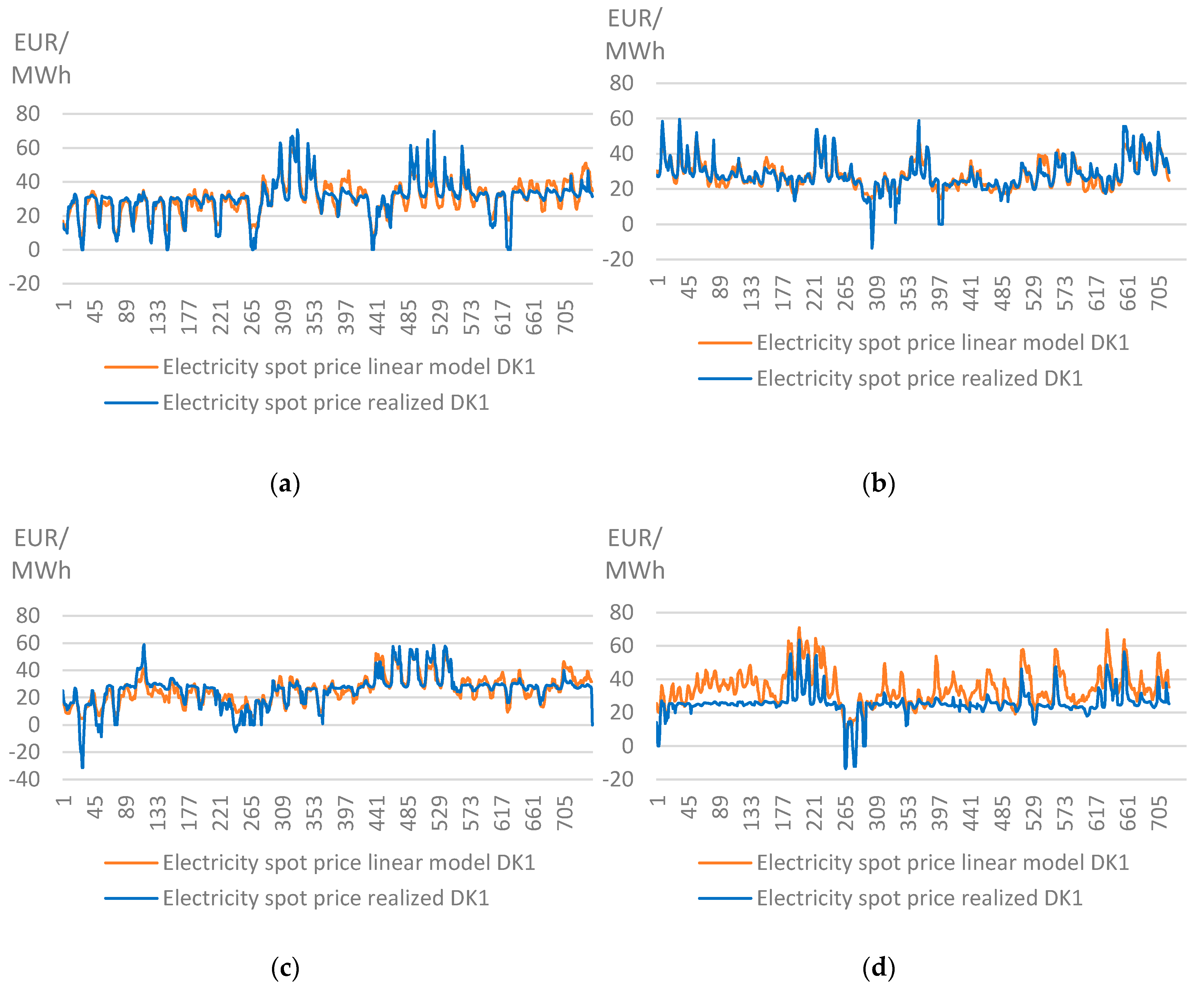
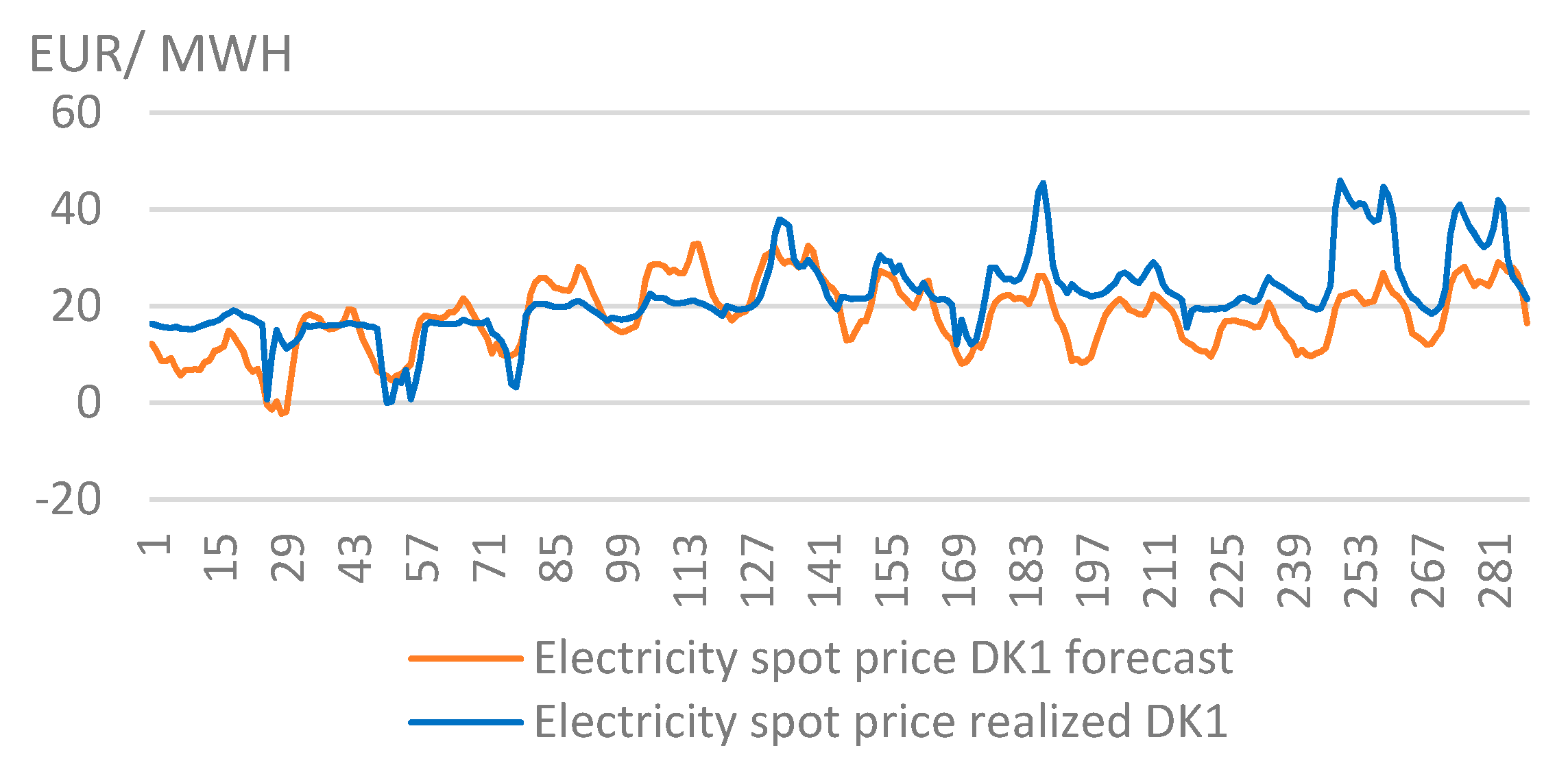
Below (Figure 2), the realized and modeled electricity spot prices with a linear model are shown for power consumption, thermal power production and previous prices.

The summary statistics of the modeled and realized electricity spot prices were calculated. The results are shown in

Table 3. Summary statistics for realized and modeled electricity spot prices.

EUR/MWH	January-14		April-14		January-15		April-15
	Real	Model	Real	Model	Real	Model	Real	Model
Sample size	744	744	720	720	744	744	720	720
Mean	30.26	30.26	28.13	28.13	25.75	25.75	25.52	25.52
Std. Deviation	11.08	9.77	8.93	7.77	11.84	10.29	7.87	6.37
Variance	122.85	95.39	79.70	60.36	140.18	105.97	61.99	40.62
Min	−0.05	7.23	−13.49	14.44	−31.41	4.35	−13.42	12.05
Max	70.68	61.28	59.60	48.60	58.84	52.47	63.49	51.46

below.

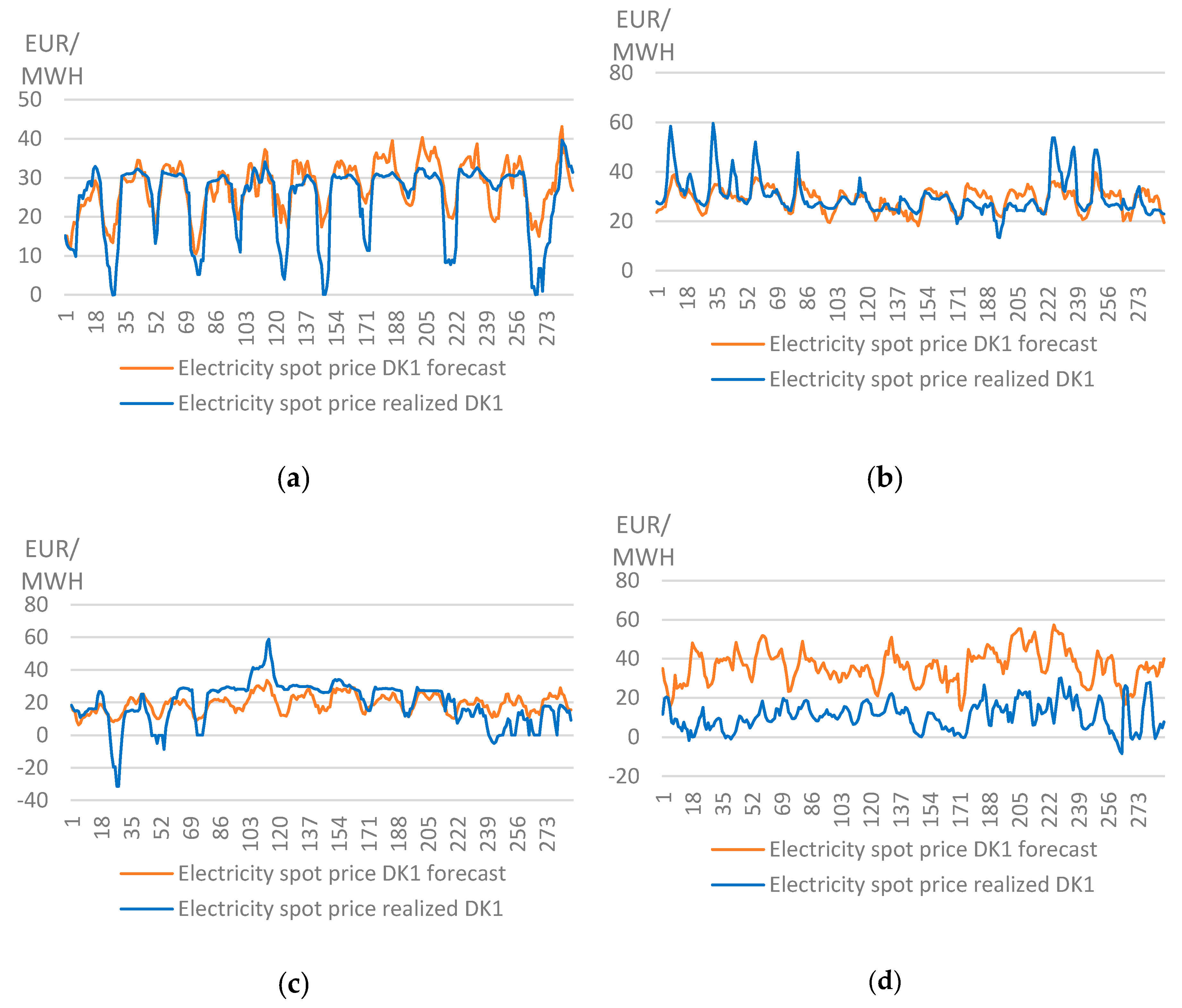
The summary statistics in Table 3 show that the mean of the linear model is identical with the realized electricity spot price. The linear model does not detect all of the spikes and drops (i.e., positive and negative price jumps), resulting in a lower variance and lower standard deviation than the realized electricity spot price. See Appendix D for the estimated parameters for the explanatory variables.

3.3. The Linear Forecasting Model

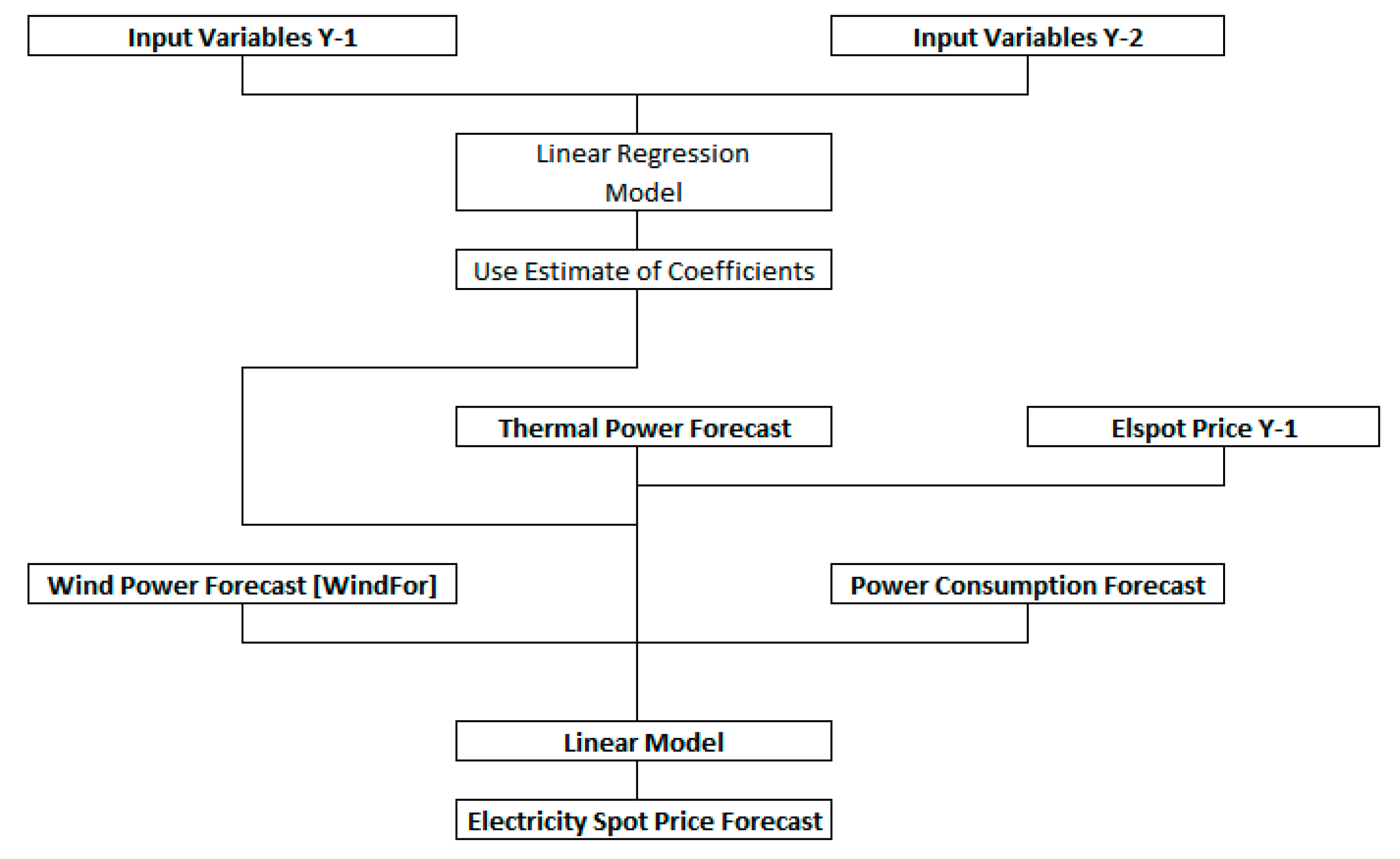
Using the linear model to forecast the electricity spot price requires a forecast of the power consumption and power production. The power consumption in this context is wind power production and thermal power production, as an analysis of the main price drivers showed that solar power production is statistically non-significant. The overall description of the model is presented in Figure 3.

The model uses a linear regression analysis to estimate the coefficients of the input variables, which are used to describe the electricity spot price. The input data consists of historical power consumption, wind power production, thermal power production and electricity spot prices.

After the coefficient has been estimated, three different forecasts are used as inputs in the electricity spot price forecast. The wind power forecast is multiplied by the coefficient of wind power production, the thermal power forecast by the coefficient of thermal power production, the power consumption forecast by the coefficient of wind power and the electricity spot price the year before with the corresponding coefficient. The method for forecasting power consumption is presented in the next section.

3.3.1. Forecasting Power Consumption

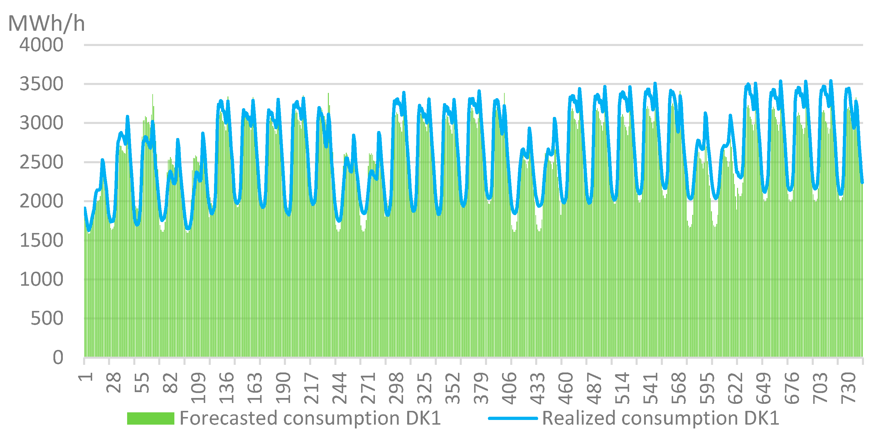
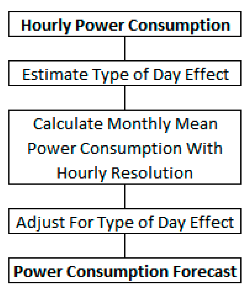
The prediction of power consumption is based on average values for a specific month of year over the past 10 years. The average power consumption for the month of January over the 10-year period is calculated, and then calendar effects are multiplied to give a forecasted consumption for the month of interest. Including the calendar effects of a month of year to the power consumption, as suggested in the literature [8,29], the demand is as follows in Figure 4.

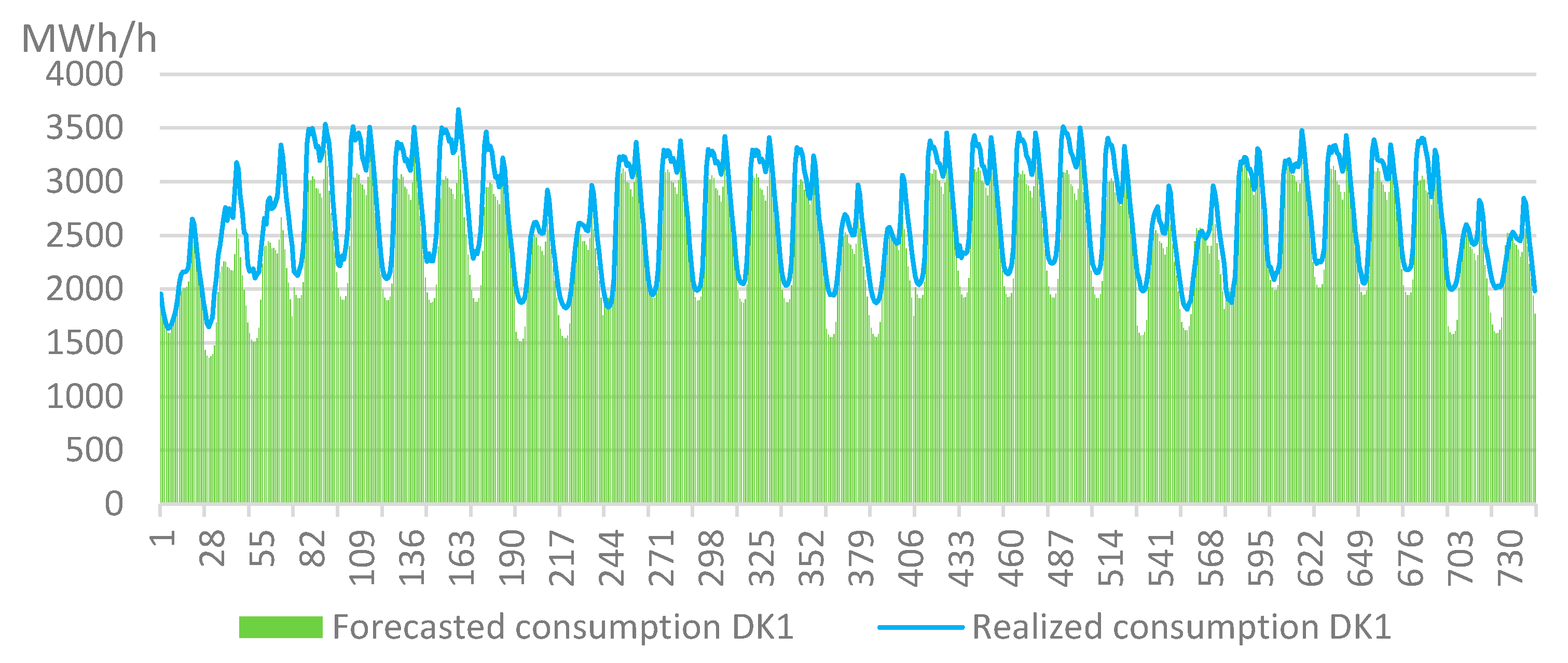
In this paper, the types of calendar effects are defined as weekend/holiday, workday, holiday not weekend, and workday after holiday. Estimating the coefficients of calendar effects was performed using the OLS method between the forecasted consumption and the realized consumption (see Appendix E for the calendar effects of the different types of days). The out-of-sample forecasts represent an average of the previous year’s coefficients. The in-sample comparison of forecasted consumption and realized consumption in DK1 can be seen in Figure 5 below. The power consumption forecasting method can be defined by the figure below (Figure 6). In the next section, the method of forecasting the power production is presented.

3.3.2. Forecasting Power Production

To forecast wind power production, WinFor (formerly known as WPPT), provided by ENFOR, was used. This model is the medium-range forecast ECMWF ensemble, consisting of 50 individual ensemble members. The model combines the data from ECMWF with the power production data from Energinet.dk. WinFor provides 5% percentile forecasts 12 days ahead. The estimated coefficients for forecasting power production (both wind and thermal) can be found in Appendix F.

Wind Power Production

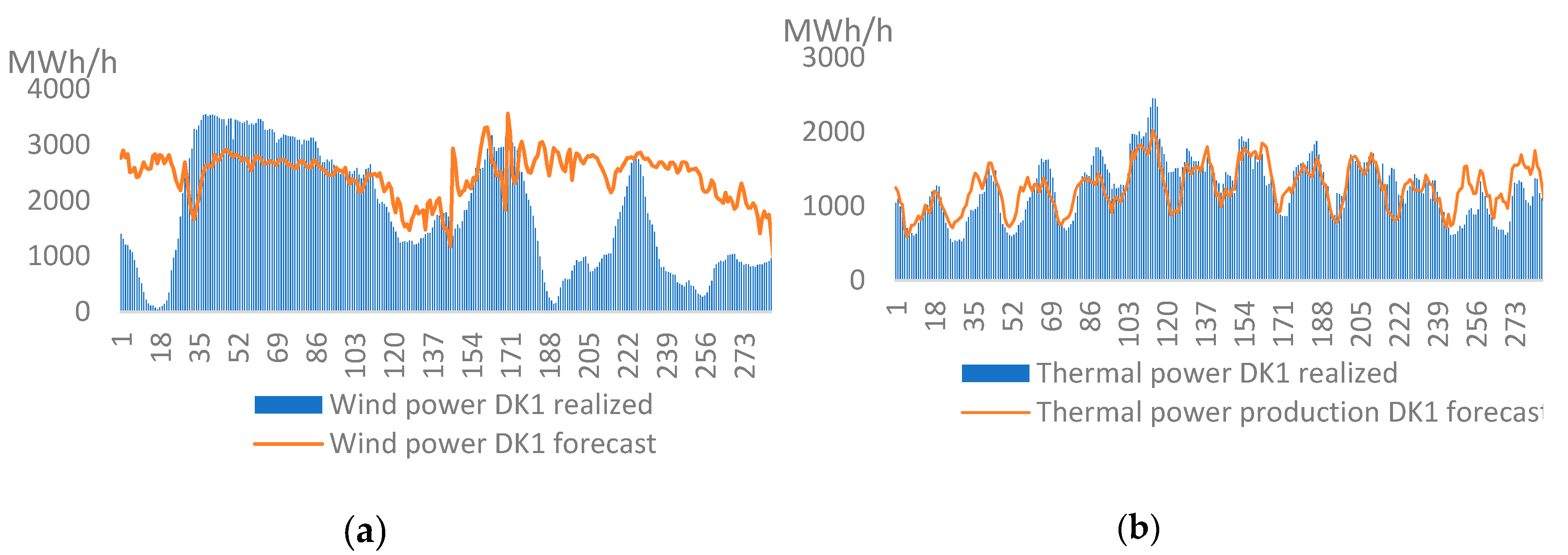
The 5% percentile WinFor model forecasts were used in a linear regression analysis to estimate the actual wind power production. The percentiles from 5% up to 95% were used in the regression model as independent variables. The figures below show the forecasts of the wind power production, compared to the realized wind power production in the four in-sample periods (see Appendix F for the coefficients).

Thermal Power Production

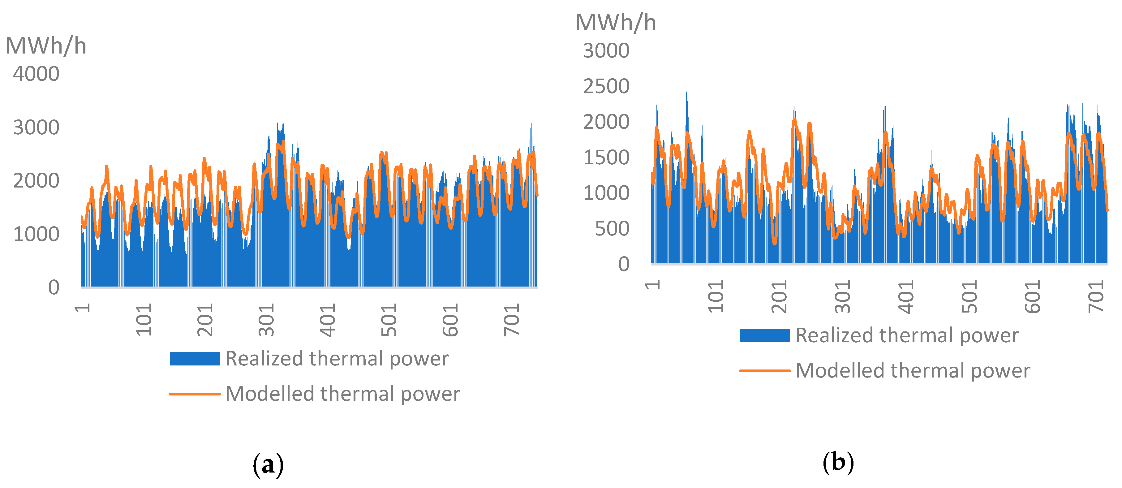
The thermal power production can be described using a linear regression model with the power consumption and wind power production as explanatory variables. From a regression analysis from January 2014, a linear model performed with an R-squared of 0.65 with power consumption and wind power production as independent variables. The coefficients can be found in Appendix F. The thermal power forecast was formed using the average of the estimated coefficients from a linear regression model of the wind power production and power consumption from the month of interest for the two years prior to the forecasting month.

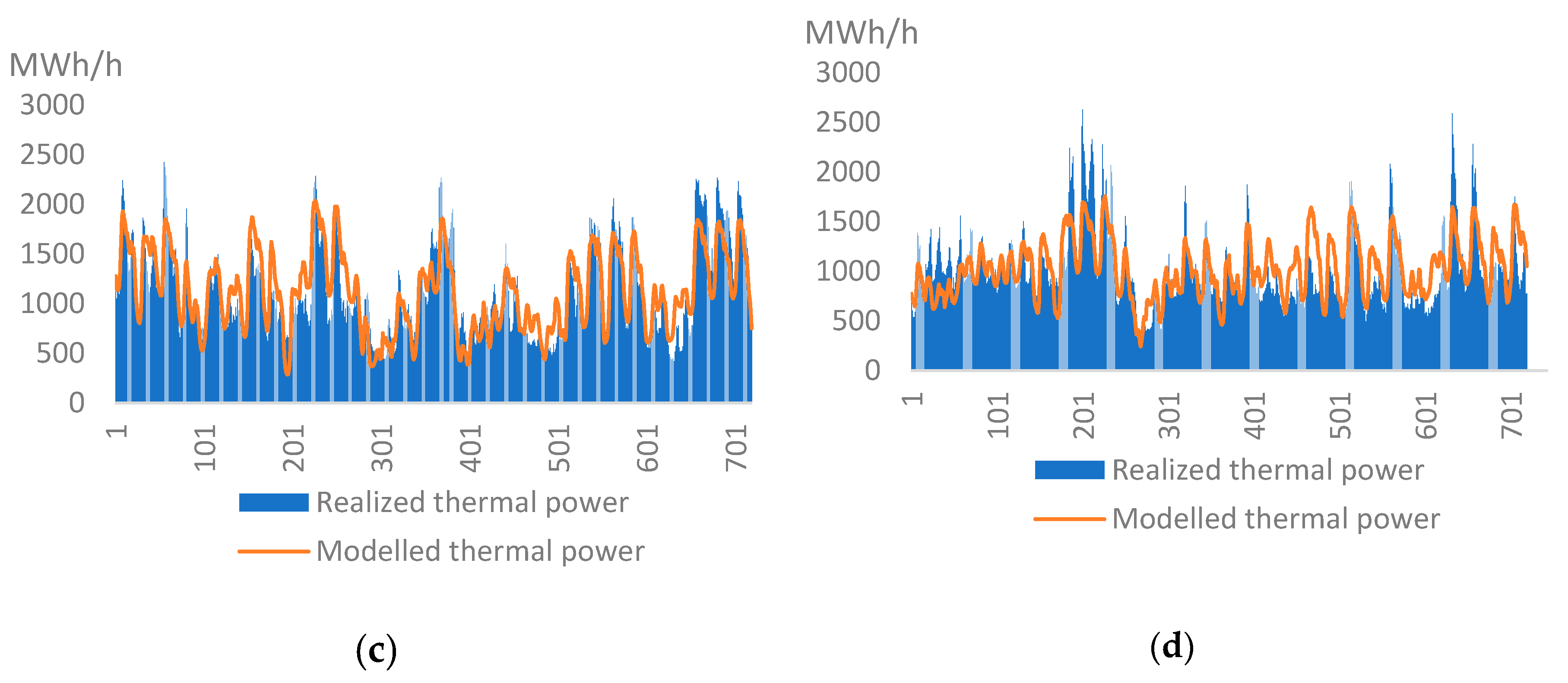
In the regression analysis from April 2014, a linear model performed with an R-squared of 0.75 with power consumption and wind power production as independent variables. The regression analysis from January 2015 reached an R-squared of 0.83, while the regression analysis from April 2015 reached an R-squared of 0.56. When using the 12-day-ahead forecast and the power consumption forecast as inputs, the modeled thermal power production reached an R-squared of 0.57 in January 2014, which is a 0.08 decrease. In April 2014, the model reached an R-squared of 0.5, which is a decrease of 0.25. In January 2015, the model reached an R-squared of 0.54, i.e., a 0.29 decrease, and the model reached an R-squared of 0.56 in April 2015, which is the same as the result of the regression analysis of the thermal power production, the actual wind power production and the actual power consumption. The out-of-sample forecast for January 2016 used an average of the coefficients of January 2014 and 2015. The last forecast performed was the price, as follows.

3.3.3. The Electricity Spot Price

The linear model with estimated parameters from the linear modeling of the electricity price with power production, power consumption and previous prices as explanatory variables is presented in the Figure 7 for the four in-sample periods. The parameters are shown in

Table 4. Summary statistics for realized and in-sample forecasted electricity spot price.

EUR/MWH	January-14		April-14		January-15		April-15
	Real	Model	Real	Model	Real	Model	Real	Model
Sample size	288	288	288	288	288	288	288	288
Mean	24.38	24.49	28.92	29.84	19.15	19.35	36.13	10.84
Std. Deviation	6.49	9.31	4.58	7.46	5.52	12.95	8.64	7.10
Variance	42.10	86.62	20.99	55.62	30.45	167.69	74.64	50.36
Min	7.23	−0.05	18.15	13.32	6.17	−31.41	13.56	−8.36
Max	40.01	39.66	39.72	59.60	33.57	58.84	57.34	30.24

.

Table 4 below presents the summary statistics for the forecasted electricity spot price and realized electricity spot price.

Table 4 shows that the January 2014, April 2014 and January 2015 forecasts provide precise predictions of the average electricity spot price for the period. April 2015, on the other hand, did not perform well when comparing the forecast and realized average electricity spot prices. Since the model cannot predict low prices particularly well, a general lack of variance is seen for the three first forecasts.

3.3.4. Model Evaluation of In-Sample Forecasts

In this section, the model presented is evaluated using the metrics from the previous section. From the metrics used to evaluate the model, April 2014 performed best with the lowest RMSE (4.22) and MAPE (13.42%), and a relatively low MAE (−0.93) compared to the other months. January 2014 performed best when considering the MAE (−0.12) and with a relatively low RMSE (4.52) as well. April 2015 was the worst-performing forecast, with a high MAE (25.29), RMSE (25.42) and MAPE (1541.41%) compared to the other in-sample forecasts.

3.3.5. Out-of-Sample Forecasts

In the following section, an out-of-sample prediction is performed, based on the proposed model in this paper. Data from the first half of January 2016 was used, and the calendar effects are summarized in

Table 5. Coefficients of calendar effects on consumption (type of day), 2014, 2015 and out-of-sample 2016.

Consumption DK1	2014		2015		2016
Month	January	April	January	April	January
Weekend/holiday	0.823	0.854	0.77	0.824	0.7965
Workday	1.006	1.047	0.954	1.028	0.98
Holiday not weekend	0.926	0.876	0.93	0.851	0.928
Day after holiday	0.957	0.948	0.911	0.914	0.934

.

Figure 8 was forecasted using the same method as mentioned in Section 3.3.1. The type-of-day effect coefficients used for forecasting the power consumption in the out-of-sample period are shown in Table 5. An out-of-sample comparison of the forecasted power consumption and the realized power consumption in DK1 can be seen in Figure 9.

Wind power production forecasts were conducted using the WinFor 5% percentile forecasts, which were also combined to forecast the thermal power production in the month of interest.

Using the forecasts shown in Figure 9, the electricity spot price forecast was constructed and is presented in Figure 10.

The estimation of the coefficients of the out-of-sample forecast is an average of the two in-sample forecast coefficients from January (see

Table 6. Estimated coefficients of power consumption, wind power production and thermal power production, including the January and April 2014/15 electricity spot prices, to forecast the out-of-sample electricity spot price, January 2016.

Elspot DK1	2014		2015		2016
Month	January	April	January	April	January
Consumption	0.00327	0.00191	−0.00060	0.00720	0.00134
Wind power	−0.00326	−0.00217	−0.00068	−0.00681	−0.00197
Thermal power	0.01270	0.01349	0.01661	0.01533	0.01465
Previous price	0.17863	0.03121	0.11946	−0.02174	0.14905
Constant	−0.57126	10.16966	−1.62510	12.48431	−1.09818

below for the coefficients).

3.3.6. Out-of-Sample Forecast Results

Evaluating the out-of-sample performance of the model concludes that it is similar to the in-sample performance in terms of the first three forecasts. The model predicted the average electricity spot price lower than the realized, and the RMSE is in the same range as the in-sample predictions when excluding April 2015 from the comparison, as shown in

Table 7. Out-of-sample forecast results compared with in-sample forecast results.

Error Measure	2014		2015		2016
Month	January	April	January	April	January
MAE	−0.12	−0.93	−0.20	25.29	−4.03
RMSE	4.52	4.22	8.30	25.42	6.22
MAPE	524.94%	13.42%	1884.0%	1541.41%	235.29%

.

4. Discussion

The complexity of the forecasting models available for forecasting electricity spot prices generally increases when using more sophisticated methods, such as neural networks and support vector machines. This complexity leads to a greater demand for computational power, as well as an increased demand for data points to be considered.

This paper presents a simple statistical method with explanatory variables for forecasting the electricity spot prices based on historical data used to estimate parameters and a wind power production forecast. The forecasting model can predict the electricity spot price based on a wind power production forecast for DK1, an electricity consumption forecast for DK1 and previous prices for the year before. The wind power production and electricity consumption forecasts are used to predict the DK1 thermal power production. The estimation of parameters was performed based on the coefficients of a linear regression analysis from the same month of interest the two previous years.

From the analysis of the electricity spot price with power production, power consumption and previous prices as explanatory variables, the linear regression model provides an R-squared on average of 0.73 and an RMSE of 4.26. When forecasting the electricity spot prices over a 12-day period, the model provides an in-sample RMSE of 4.52 for January 2014 and an out-of-sample RMSE of 6.22 for January 2016. When using an ARX model, the regression results reach 0.87–0.88 for a day-ahead forecasting [10]. Using a seasonal neural network approach for 72-h-ahead forecasting [22] presented a model with an overall RMSE of 1.46 for the period, which is more than four times greater than the simple linear model, but the forecasting period is also four times shorter than the forecasting period for the simple linear model.

The artificial neural network approach provides a one-hour-ahead forecast with a MAE of 1.44 and an RMSE of 1.92 [17]. The simple linear model provides an in-sample MAE of −0.12 and out-of-sample MAE of −4.04. The results from the comparative analysis are interesting, as: (1) they provide an overview of which forecasting models to use for which scenarios; (2) improved forecasting models are likely to increase the accuracy in energy supply assessments, thereby improving the grid operator’s ability to plan for additional renewable energy input and, finally, (3) they support the continuation of new wind farm installations aimed at meeting the global climate target.

5. Conclusions

The increase of power production based on renewable energy sources—wind especially—has made it more complicated to forecast electricity prices. This study has examined the country with the highest share of wind power production in the combined energy system, namely Denmark. The Danish electricity market is highly dependent on the performance of the country’s wind farms, which naturally affects electricity prices. Various forecasting models have been considered for best-practice forecasting, and a method requiring little to no computational resources has been proposed.

Many of the models are linear models based on statistics that are more sophisticated, whereas this paper tests a simple linear regression model to perform electricity spot price forecasts for a 12-day period. From the linear regression analysis, the main price drivers were found to be exchange rates between DK1 and the neighbor areas, as well as power production in DK1, such as wind power, thermal power and the demand for electricity in DK1.

This paper proposes a simple linear model to forecast the electricity prices 12 days ahead with hourly resolution, with significantly larger errors than the models presented in the literature, but the simple model provides hourly price forecasts for 4–12 times longer forecasting horizons than the models in the literature.

These results mean that grid operators, energy traders etc. can estimate prices with an hourly resolution up to 12 days ahead, which supports the continuous development of wind power, as such knowledge can guide storage technologies and other ancillary services.

References

- Danish Energy Agency. Overview over the Energy Sector—ens.dk. 2017. Available online: https://ens.dk/service/statistik-data-noegletal-og-kort/data-oversigt-over-energisektoren (accessed on 6 December 2019).
- International Energy Agency. Denmark: Electricity and Heat for 2005 to 2018—iea.org. 2018. Available online: https://www.iea.org/data-and-statistics/data-tables?country=DENMARK&energy=Electricity&year=2018 (accessed on 26 November 2019).
- Jónsson, T.; Pinson, P.; Nielsen, H.; Madsen, H. Exponential smoothing approaches for prediction in real-time electricity markets. Energies 2014, 7, 3710–3732. [Google Scholar] [CrossRef] [Green Version]
- Weron, R. Electricity price forecasting: A review of the state-of-the-art with a look into the future. Int. J. Forecast. 2014, 30, 1030–1081. [Google Scholar] [CrossRef] [Green Version]
- Hou, P.; Enevoldsen, P.; Eichman, J.; Hu, W.; Jacobson, M.Z.; Chen, Z. Optimizing investments in coupled offshore wind: Electrolytic hydrogen storage systems in Denmark. J. Power Sources 2017, 359, 186–197. [Google Scholar] [CrossRef]
- Karabiber, O.A.; Xydis, G. Electricity price forecasting in Danish day-ahead market using TBATS, ANN and ARIMA methods. Energies 2019, 12, 928. [Google Scholar] [CrossRef] [Green Version]
- Shahidehpour, M.; Yamin, H.; Li, Z. Market Operations in Electric Power Systems: Forecasting, Scheduling, and Risk Management, 1st ed.; Wiley: Chichester, UK, 2002. [Google Scholar]
- Lucia, J.J.; Schwartz, E.S. Electricity prices and power derivatives: Evidence from the Nordic Power Exchange. Rev. Deriv. Res. 2002, 5, 5–50. [Google Scholar] [CrossRef]
- Weron, R.; Misiorek, A. Forecasting spot electricity prices: A comparison of parametric and semiparametric time series models. Int. J. Forecast. 2008, 24, 744–763. [Google Scholar] [CrossRef] [Green Version]
- Kristiansen, T. Forecasting Nord Pool day-ahead prices with an autoregressive model. Energy Policy 2012, 49, 328–332. [Google Scholar] [CrossRef]
- Kristiansen, T. A time series spot price forecast model for the Nord Pool market. Int. J. Electr. Power Energy Syst. 2014, 61, 20–26. [Google Scholar] [CrossRef]
- Knapik, O. Essays on Econometric Modelling and Forecasting of Electricity Prices; Center for Research in Econometric Analysis of Time Series: Aarhus, Denmark, 2017. [Google Scholar]
- Janczura, J.; Weron, R. An empirical comparison of alternate regime-switching models for electricity spot prices. Energy Econ. 2010, 32, 1059–1073. [Google Scholar] [CrossRef] [Green Version]
- Karakatsani, N.; Bunn, D.W. Fundamental and behavioural drivers of electricity price volatility. Stud. Nonlinear Dyn. Econ. 2010, 4. [Google Scholar] [CrossRef]
- Russel, J. Econometric Analysis of Irregularly-Spaced Transaction Data Using a New Class of Accelerated Failure Time Models with Applications to Financial Transaction Data. Ph.D. Thesis, University of California, San Diego, CA, USA, 1996. [Google Scholar]
- Russell, J.R.; Engle, R. A discrete-state continuous-time model of financial transactions prices and times: The autoregressive conditional multinomial: Autoregressive conditional duration model. J. Bus. Econ. Stat. 2005, 2, 166–180. [Google Scholar] [CrossRef]
- Kurbatsky, V.G.; Sidorov, D.N.; Spiryaev, V.A.; Tomin, N.V. Forecasting nonstationary time series based on Hilbert-Huang transform and machine learning. Autom. Remote Control 2014, 75, 922–934. [Google Scholar] [CrossRef]
- Panagiotidis, P.; Effraimis, A.; Xydis, G. An R-focused forecasting approach for efficient demand response strategies in autonomous micro grids. Energy Environ. 2019, 30, 63–80. [Google Scholar] [CrossRef] [Green Version]
- Huang, N.E.; Shen, Z.; Long, S.R.; Wu, M.C.; Shih, H.H.; Zheng, Q.; Yen, N.-C.; Tung, C.C.; Liu, H.H. The empirical mode decomposition and the Hilbert spectrum for nonlinear and non-stationary time series analysis. In Proceedings of the Royal Society of London. Series A: Mathematical, Physical and Engineering Sciences; The Royal Society: London, UK, 1998; Volume 1971, pp. 903–995. [Google Scholar]
- Cortes, C.; Vapnik, V. Support-vector networks. Mach. Learn. 1995, 3, 273–297. [Google Scholar] [CrossRef]
- Tay, F.E.H.; Cao, L. Application of support vector machines in financial time series forecasting. Omega 2001, 4, 309–317. [Google Scholar] [CrossRef]
- Saâdaoui, F. A seasonal feedforward neural network to forecast electricity prices. Neural Comput. Appl. 2017, 28, 835–847. [Google Scholar] [CrossRef]
- Parsons, B.; Milligan, M.; Zavadil, B.; Brooks, D.; Kirby, B.; Dragoon, K.; Caldwell, J. Grid impacts of wind power: A summary of recent studies in the United States. Wind Energy 2004, 2, 87–108. [Google Scholar] [CrossRef]
- Hong, T.; Pinson, P.; Fan, S. Global energy forecasting competition 2012. Int. J. Forecast. 2014, 2, 357–363. [Google Scholar] [CrossRef]
- Nguyen, T.N. A different approach to information management by exceptions (toward the prevention of another Enron). Inf. Manag. 2014, 51, 165–176. [Google Scholar] [CrossRef]
- Jónsson, T.; Pinson, P.; Madsen, H. On the market impact of wind energy forecasts. Energy Econ. 2010, 2, 313–320. [Google Scholar] [CrossRef] [Green Version]
- Ketterer, J.C. The impact of wind power generation on the electricity price in Germany. Energy Econ. 2014, 44, 270–280. [Google Scholar] [CrossRef] [Green Version]
- Draper, N.R.; Smith, H. Applied Regression Analysis, 3rd ed.; Wiley: New York, NY, USA, 1998. [Google Scholar]
- Moral-Carcedo, J.; Pérez-García, J. Integrating long-term economic scenarios into peak load forecasting: An application to Spain. Energy 2017, 140, 682–695. [Google Scholar] [CrossRef]
Figure 1.
Danish annual power production per type, 2005–2018 [2].
Figure 2.
The electricity spot price realized compared with the linear regression model. (a) shows data for January 2014, (b) April 2014, (c) January 2015 and (d) April 2015.
Figure 3.
Overview of the linear forecasting model.
Figure 4.
In-sample forecast of power consumption compared to realized consumption in the Danish electricity market (DK1), January 2014.
Figure 5.
Thermal power production modeled as a function of power consumption and wind power production compared to the realized thermal power production. (a) shows data for January 2014, (b) April 2014, (c) January 2015 and (d) April 2015.
Figure 6.
Power consumption forecasting method.
Figure 7.
Electricity spot price forecast based on the linear regression model compared to the realized electricity spot price. The top-left shows data for January 2014 (a), the top-right April 2014 (b), the bottom-left January 2015 (c) and the bottom-right April 2015 (d).
Figure 8.
Out-of-sample forecast of power consumption compared with realized consumption in DK1, January 2016.
Figure 9.
(a) Shows wind power production forecast in DK1, January 2016, based on WinFor percentile forecast. (b) Shows thermal power production forecast in DK1, January 2016, based on forecasted power consumption and WinFor percentile forecast.
Figure 10.
Out-of-sample forecast of the electricity spot price in DK1 for the first half of January 2016.