Determining Soil Hydraulic Properties Using Infiltrometer Techniques: An Assessment of Temporal Variability in a Long-Term Experiment under Minimum- and No-Tillage Soil Management

Abstract

Conservation agriculture is increasingly accepted by farmers, but the modeling studies on agro-environmental processes that characterize these agricultural systems require accurate information on the temporal variability of the soil’s main physical and hydraulic properties. Therefore, specific investigations carried out in long-term experiments can increase our knowledge on the pros and cons of different measurement techniques. In this work, the simplified falling head (SFH) technique and the Beerkan Estimation of Soil Transfer (BEST) procedure were applied to investigate the temporal variability of some main soil physical and hydraulic properties, including bulk density (BD), field saturated hydraulic conductivity (K_fs), macroporosity (P_mac), air capacity (AC), plant available water capacity (PAWC), and relative field capacity (RFC). For this purpose, a long-term experiment was selected, and the experimental information obtained was used to verify the long-term impact (fifteen years) determined by two alternative forms of soil management, minimum tillage (MT) and no tillage (NT), for the cultivation of durum wheat. The main results of the comparison between MT and NT showed: (i) A comparable temporal variability in K_fs values when SFH was considered, given that in 75% of considered cases, the same result (i.e., significant or not significant) was obtained; (ii) a comparable temporal variability in K_fs values under MT (but not under NT) when both SFH and BEST were used, as a result of a possible K_fs,SFH overestimation under NT; (iii) differences in K_fs estimations by a factor of 6 or 7 (K_fs,SFH > K_fs,BEST) when comparable soil conditions (moisture and soil density) were considered; (iv) a comparable temporal variability when other soil indicators (BD, P_mac, AC, PAWC, and RFC) were simultaneously considered. After about fifteen years of field experiments characterized by continuous soil management and conducted with the methodological rigor typical of experimental farms, the SFH- and BEST-derived experimental information showed a substantial equivalence between MT and NT for the fine-textured soil investigated.

1. Introduction

The soil hydraulic properties (i.e., water retention and hydraulic conductivity) are key information in many fields of agro-environmental research works, since they are necessary, for example, for simulating a few agro-environmental processes [1,2,3], for establishing agronomic adaptation strategies under climate change [4,5,6], and for quantifying economic and environmental impacts of alternative soil management [7,8,9,10].

Many techniques are available in the literature for obtaining the hydraulic soil properties that differ in accuracy, specific skills for their application, and experimental efforts (costs and execution times). Some techniques provide discrete values of soil properties, e.g., soil water retention at field capacity or saturated hydraulic conductivity, while other techniques can generate continuous hydraulic property data. For instance, the evaporation method is widely used because it provides accurate estimations of soil hydraulic properties [11], but requires sampling of undisturbed soil cores and relatively laborious and time-consuming lab procedures. Consequently, the use of simplified and expeditious methods is increasingly frequent, and the choice of the most appropriate one depends on specific experimental needs and economic availability.

The simplified falling head (SFH) technique by Bagarello et al. [12] allows the estimation of the field saturated hydraulic conductivity (K_fs) in a sufficiently accurate and repeatable way with relatively limited experimental effort. For these potentialities, it has been widely used to obtain K_fs in specific agro-environmental investigations on both herbaceous [13] and arboreal [14] agronomic crops. A literature review also revealed that the SFH technique was successfully applied to investigate the influence of soil compaction on water infiltration rate due to cattle hooves or tractors [15], to assess soil hydraulic quality factors and develop a comprehensive soil quality index under different cropping systems [16], to study the soil physical quality response to sugarcane expansion in Brazil [17], and to investigate the impact of herbicide glyphosate on compost-amended soils [18].

The Beerkan Estimation of Soil Transfer (BEST) parameters procedure by Lassabatère et al. [19] is an attractive, easy, robust, and inexpensive way for a “complete” soil hydraulic characterization, since it allows the simultaneous determination of the water retention curve, h(θ), and the hydraulic conductivity function, K(θ) [20]. The BEST method has shown reliability and robustness based on several theoretical and experimental evaluations; consequently, in recent years, it was applied for soil property estimation in agro-environmental sustainability investigations [21,22,23,24,25]. For instance, BEST was applied by Yang et al. [21] in a karst landscape of southern China to investigate the effects of Napier grass management on soil hydrological functions and to identify reasonable strategies for maintaining optimal soil hydraulic functions. Yang et al. [22] used this method to establish the impact of different vegetation restoration types on K_fs within a large global ecological restoration engineering project. Likewise, the impact of native, spontaneous, or exotic vegetation on soil hydraulic properties was assessed by BEST in areas of France [23] and Brazil [24]. Di Prima et al. [25] applied BEST to investigate the soil physical quality of a Spanish orchard under three different soil management types, i.e., no-tillage using herbicides, conventional tillage under chemical farming, and no-tillage under organic farming. The results showed that independent and BEST-derived indicators (i.e., soil bulk density, total organic carbon, and structure stability index, in conjunction with plant available water, relative field capacity, and saturated hydraulic conductivity) yielded similar information, suggesting their ability to distinguish soil qualities among contrasting soil management types.

Soil hydraulic properties are highly variable in space and time [26,27,28], and several sampling times are needed to investigate the seasonal, or temporal, variability during a crop cycle, or between sampling dates of different cropping years [29]. Overall, there is a wide literature on the temporal variability of soil physical and hydraulic properties, as well as on the effects induced by the practices applied in agriculture. For instance, Castellini et al. [29] investigated the seasonal variability of the water retention curve and the relative field capacity of the soil under different soil management types (i.e., no-tillage, minimum tillage, and incorporation into the soil of wheat straw). The results showed that there was no seasonal variability from about February until June, suggesting that four or five months are the minimum times required after the last soil disturbance to reach near-optimal physical quality of the soil. Kreiselmeier et al. [28] studied the temporal changes of soil hydraulic conductivity (both saturated and unsaturated) under conventional and conservation tillage. The findings showed a high temporal variability of K_fs in tilled soils (lower under unsaturated soil condition) and a greater stability of K_fs in untilled soils, confirming the susceptibility of tilled soils to variations, also in the short term. However, to the best of our knowledge, although the literature on this topic is very extensive, specific investigations aimed at comparing the temporal variability estimated by two different infiltrometric techniques have not yet been carried out. Therefore, the two cited techniques (SFH and BEST) could be applied simultaneously to investigate the seasonal (or temporal) variability of specific soil management and to evaluate the respective pros and cons.

The no-tillage of the soil, as compared with traditional plowing or various options of minimum tillage, has received growing interest in cereal cropping systems in southern Italy. This is true especially for wheat cultivation, since no tillage is increasingly considered as a real alternative to soil tillage [30]. However, according to a hydrological perspective aimed at assessing the impact of these two soil management systems on soil hydrology and water conservation, appropriate case studies should be shared in order to generalize, to a certain extent, the information obtained [28,31,32].

Long-term field experiments, carried out in the experimental farms of the research institutes or universities, represent important research tools to assess, for example, the temporal variability of selected soil properties given that (i) relatively stable conditions can be expected in these soils and (ii) the cultivation operations are carried out with scientific rigor [31,33,34]. Consequently, these factors provide the basis to obtain robust experimental information.

The general objective of this investigation was to assess the temporal variability of physical and hydraulic properties of a fine-textured soil in a long-term experiment (about fifteen years) for durum wheat cultivation under minimum tillage (MT) and no tillage (NT). The specific objectives were to: (i) Apply the SFH and BEST methods to obtain the main physical and hydraulic properties of the soil (i.e., bulk density, saturated hydraulic conductivity, macroporosity, air capacity, plant available water capacity, relative field capacity); (ii) investigate the temporal variability obtained by the selected methods; (iii) compare the estimations obtained by SFH and BEST; (iv) use the acquired experimental information to assess the agro-environmental sustainability of MT and NT from the perspective of soil physical and hydraulic properties.

2. Materials and Methods

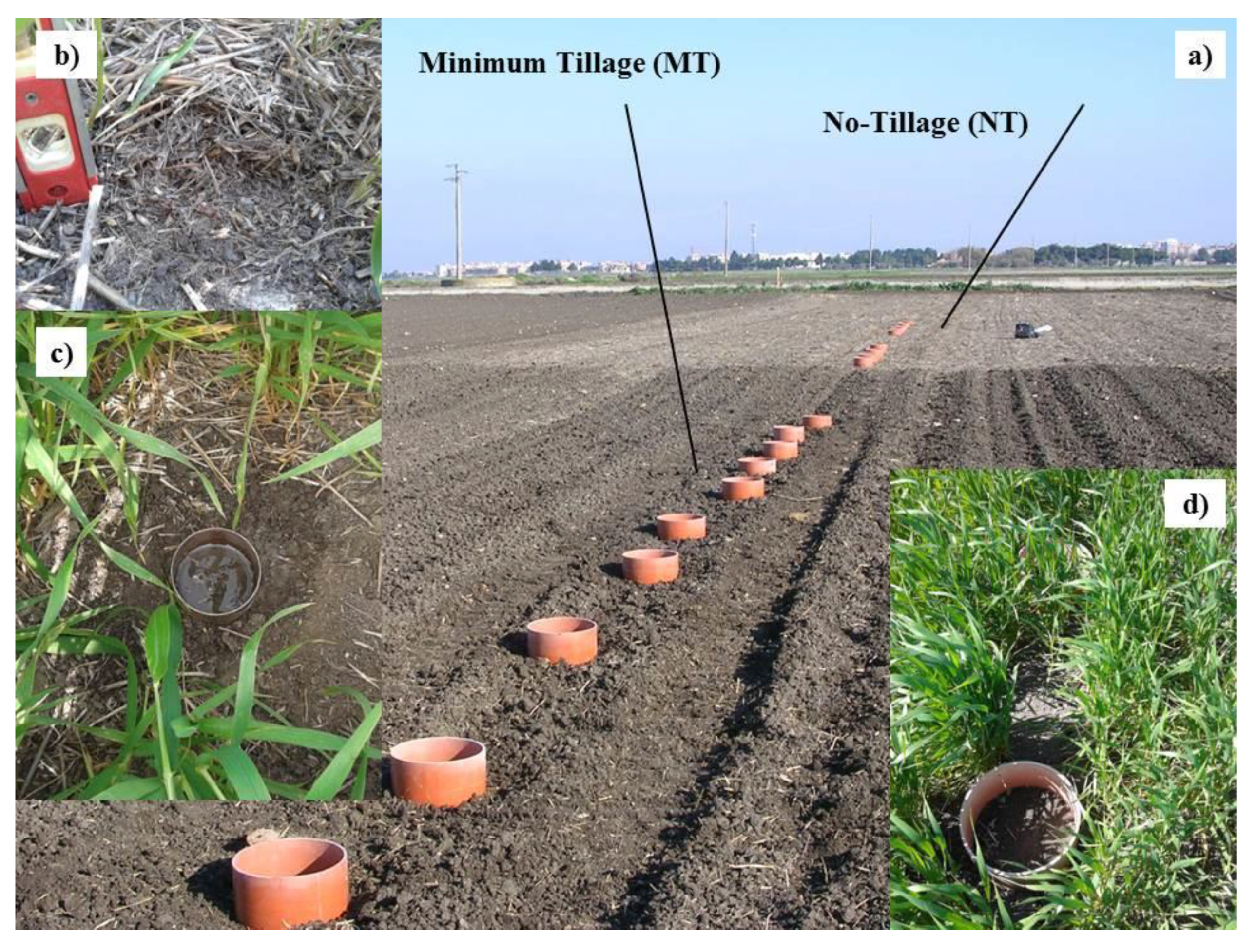
2.1. Experimental Site

The study was carried out in the two-year period of 2016–2017 at the experimental farm of the Council for Agricultural Research and Economics, CREA-AA, Foggia (41°27′03” N, 15°30′06” E), in a long-term field experiment performed on a monoculture of durum wheat (Triticum durum, Desf.). The study, started in 2002, aims at comparing the effects of tillage (minimum tillage, MT) and sod-seeding (no tillage, NT) on grain yield and quality. The experimental design is a completely randomized block design with three replicates and unit plots of 500 m² size (Figure 1a). Straw was chopped into 10–15 cm lengths and spread back on the plot in September (first week); this resulted in about 40–50 q/ha of organic matter returned to the soil (Figure 1b). A two-layer tillage (field cultivator with rotary tiller) was carried out in the MT plots (late October–early November). For the NT plot, chemical weed control and direct sowing were carried out. Sowing was performed in early November. According to the USDA classification, the soil texture is that of clay, with 42.7% and 27.7% of clay and silt, respectively [32]. As an example, an image of the experimental site is shown in Figure 1.

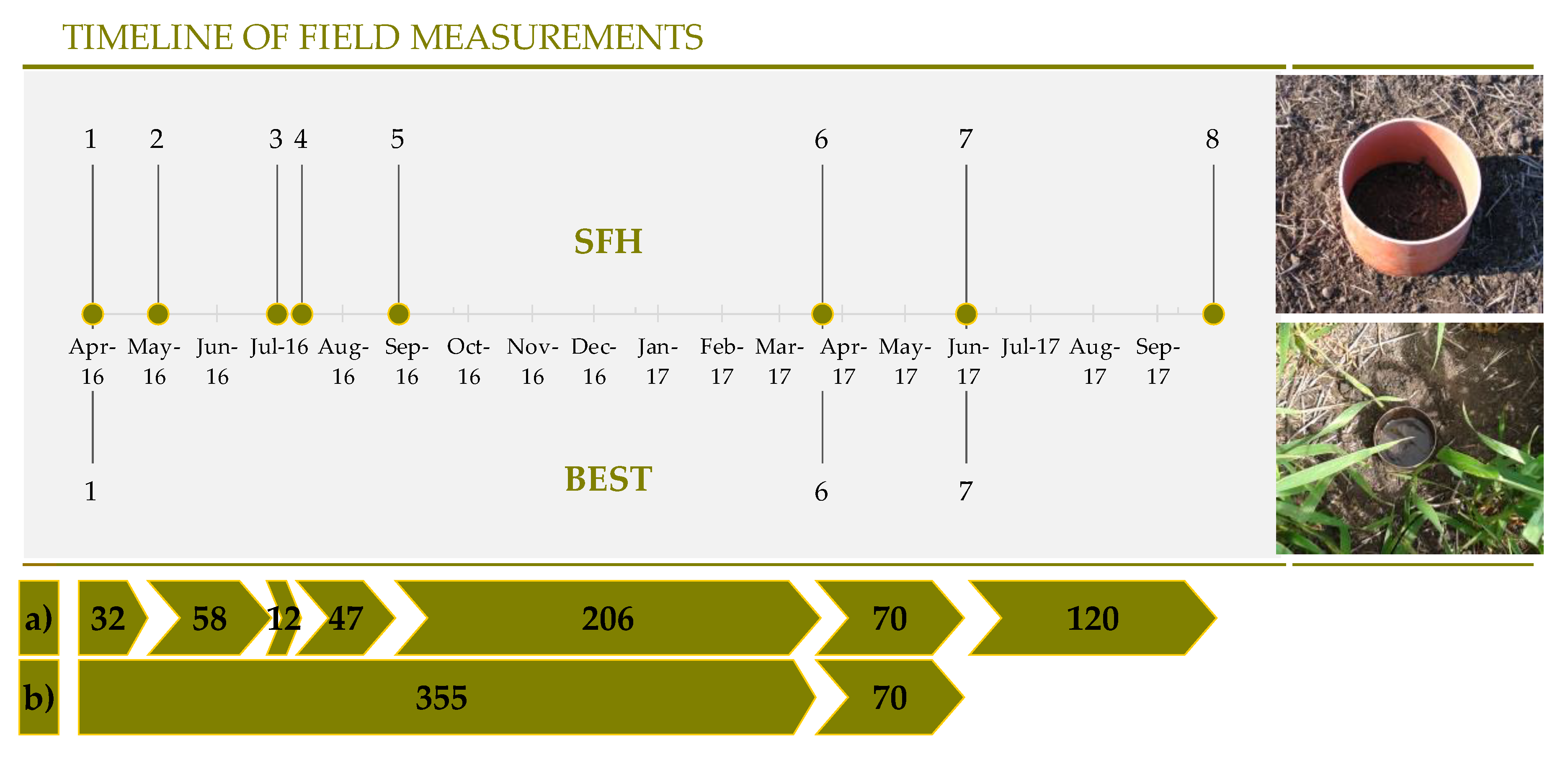
2.2. Simplified Falling Head (SFH) Technique

The SFH technique [12] consists of quickly pouring a known volume of water, V (L³), onto the soil confined inside a ring inserted at a fixed depth into the soil, d (L), and measuring the time, t_a (T), necessary for the poured volume, Δθ (equal to the volume of water obtained by difference between the soil water content at saturation, θ_s, and that at the time of the experiment, θ_i), to fully seep through to the surface area, A (L²). In other words, given a value of the water content at the beginning of the experiment, Δθ represents the amount of water needed to saturate the soil porosity estimated at the time of sampling. The K_fs values were determined by a one-dimensional, transient, falling-head infiltration process, based on the analysis by Philip [35]:

$$K_{fs,SFH}=\frac{\left(\Delta \theta \right)}{\left(1-\Delta \theta \right)t_a}\left[\frac{D}{\left(\Delta \theta \right)}-\frac{\left(D+\frac{1}{{\alpha }^{*}}\right)}{\left(1-\Delta \theta \right)}\ln \left(1+\frac{\left(1-\Delta \theta \right)D}{\left(\Delta \theta \right)\left(D+\frac{1}{{\alpha }^{*}}\right)}\right)\right]$$

(1)

where D = V/A (L) is the depth of water corresponding to V, and α* (L⁻¹) is a soil texture/structure parameter. According to the procedure reported by Bagarello et al. [12], two undisturbed soil cores (5 cm in height by 5 cm in diameter) were collected near the ring at the 0 to 5 and 5 to 10 cm depth about 24 h before the measurements to determine the dry soil bulk density, BD (g cm³), and the soil water content at the time of sampling, θ_i (cm³ cm⁻³), in the laboratory. The saturated soil water content, θ_s, was estimated using the measured BD and considering a mean value of soil particle density of 2.65 g cm⁻³, as is usual for this procedure [12,36]. A choice of the most suitable α* parameter can be made following the guidelines of Elrick and Reynolds [37]. However, according to previous experimental investigations carried out on investigated soil [38], a value of the α* equal to 0.012 cm⁻¹ was used to calculate K_fs.

The SFH technique was applied in two consecutive years (growing season 2015–2016 and 2016–2017) to determine the field saturated soil hydraulic conductivity, K_fs,SFH. In particular, the SFH tests started about five months after pipe insertion; this made it possible to exclude (or attenuate) the possible compaction during cylinder insertion. Five sampling dates were considered in 2016 and another three in 2017 (Figure 2). For each considered agronomic treatment (MT and NT), ten PVC pipes of 30 cm in inner diameter and 30 cm in height (with relatively sharp edges) were inserted into the soil (in mid-November) at a depth d = 15 cm. Using the bucket loader of a tractor, the insertion of the PVC pipe was conducted step by step, ensuring that the upper rim of the pipe remained horizontal. A spirit level was used to check the horizontality of the cylinder. To obtain a flat infiltration surface, the small depressions of the cylinder’s inner area were filled with soil collected in situ. The PVC pipes were always removed immediately before the start of the next crop cycle (at the beginning of November).

2.3. Beerkan Estimation of Soil Transfer (BEST) Parameters Procedure

The BEST procedure [19] was applied to simultaneously determine the water retention curve, h(θ), and the soil hydraulic conductivity function, K(θ), of the soil. BEST focuses specifically on the van Genuchten [39] relationship with the Burdine [40] condition for the water retention curve (Equation (2a)) and the Brook and Corey [41] relationship for hydraulic conductivity (Equation (3a)):

$$\frac{\theta -{\theta }_r}{{\theta }_s-{\theta }_r}={\left[1+{\left(\frac{h}{h_g}\right)}^n\right]}^{-m}$$

(2a)

$$m=1-\frac{1}{n}$$

(2b)

$$\frac{K\left(\theta \right)}{K_{fs,BEST}}={\left(\frac{\theta -{\theta }_r}{{\theta }_s-{\theta }_r}\right)}^{\eta }$$

(3a)

$$\eta =\frac{2}{m\cdot n}+2+p$$

(3b)

where θ (L³L⁻³) is the volumetric soil water content, h (L) is the soil water pressure head, K (L T⁻¹) is the unsaturated soil hydraulic conductivity, n (>2), m, and η are shape parameters, p is a tortuosity parameter set equal to 1 following Burdine’s [40] condition, and h_g (L), θ_s (field saturated soil water content; L³L⁻³), θ_r (residual soil water content; L³L⁻³), and K_fs,BEST (field saturated hydraulic conductivity; LT⁻¹) are scale parameters. In BEST, θ_r is assumed to be equal to zero. Shape parameters, which are texture-dependent, are estimated from particle size analysis and soil bulk density measurement by assuming a shape similarity between the particle size distribution and the water retention curve [42].

To obtain the shape parameters of soil hydraulic functions, the particle size distribution (PSD) of the soil is fitted to the following equations:

$$F\left(D\right)={\left[1+{\left(\frac{D_g}{D}\right)}^N\right]}^{-M}$$

(4a)

$$M=1-\frac{2}{N},$$

(4b)

where F(D) is the fraction by mass of particles passing a particular diameter, D (L), M and N are two shape parameters, and D_g (L) is a scale parameter.

The fitting of Equation (4a) provides an estimation of parameters M, N, and D_g. The shape index of the medium, p_m, can be obtained from M and N:

$$p_m=p_M{\left(1+\kappa \right)}^{-1}$$

(5a)

$$p_m=\frac{mn}{1+m}$$

(5b)

$$p_M=\frac{MN}{1+M}$$

(5c)

where the coefficient κ is equal to:

$$\kappa =\frac{2s-1}{2s\left(1-s\right)},$$

(6)

in which s is the fractal dimension of the medium, defined as the root of the following equation:

$${\left(1-f\right)}^s+f^{2s}=1.$$

(7)

The m parameter is derived from the values of p_m considering the positive root of Equation (5b):

$$m=\frac{1}{p_m}\left(\sqrt{1+p_m{}^2}-1\right).$$

(8)

To estimate the field saturated hydraulic conductivity, K_fs,BEST, experimental data from Beerkan infiltrations and the approximations of the quasi-exact implicit infiltration model by Haverkamp et al. [26,43] were used. Specifically, when an infiltration experiment with a zero-water-pressure head on a circular surface of radius r (L) is performed under homogenous conditions of θ_i (L³ L⁻³), the 3D cumulative infiltration, I (L), and the infiltration rate, I (LT⁻¹), can be approached by the following explicit transient (Equation (9a,b)) and steady-state (Equation (9c,d)) relationships [26,43]:

$$I\left(t\right)=S\sqrt{t}+\left(A{S}^2+B{K}_s\right)t$$

(9a)

$$i\left(t\right)=\frac{S}{2\sqrt{t}}+\left(A{S}^2+B{K}_s\right)$$

(9b)

$$I_s\left(t\right)=\left(A{S}^2+K_s\right)t+C\frac{S^2}{K_s}$$

(9c)

$$i_s\left(t\right)=A{S}^2+K_s,$$

(9d)

where I_s and i_s are respectively the asymptotic models for I and i for large times, t is the time (T), and A (L⁻¹), B, and C are constants that, for the Brooks and Corey model [41] model, may be obtained as:

$$A=\frac{\gamma }{r\left({\theta }_s-{\theta }_i\right)}$$

(10a)

$$B=\frac{2-\beta }{3}\left[1-{\left(\frac{{\theta }_i}{{\theta }_s}\right)}^{\eta }\right]+{\left(\frac{{\theta }_i}{{\theta }_s}\right)}^{\eta }$$

(10b)

$$C=\frac{1}{2\left(1-\beta \right)\left[1-{\left(\frac{{\theta }_i}{{\theta }_s}\right)}^{\eta }\right]}\ln \left(\frac{1}{\beta }\right),$$

(10c)

where β and γ are coefficients that are usually set equal to 0.6 and 0.75, respectively, when θ_i < 0.25 θ_s [26,43].

The scale parameter for the van Genuchten water retention curve, h_g [L], is estimated by the following relationship:

$$h_g=-\frac{S^2}{c_p\left({\theta }_s-{\theta }_i\right)\left[1-{\left(\frac{{\theta }_i}{{\theta }_s}\right)}^{\eta }\right]K_{fs,BEST}},$$

(11)

where S (LT^‒1/2) is the soil sorptivity and c_p is a coefficient dependent on n, m, and θ according to Equation (6b) by Lassabatère et al. [19].

Three alternative algorithms were developed to analyze field infiltration data, i.e., BEST-slope [19], BEST-intercept [44], and BEST-steady [26]. The BEST-slope by Lassabatere et al. [19] makes use of the following relationships for both K_fs,BEST and cumulative infiltration, I(t):

$$K_{fs,BEST}=i_s-A{S}^2$$

(12a)

$$I\left(t\right)=S\sqrt{t}+\left[A\left(1-B\right)S^2+B{i}_s\right]t,$$

(12b)

where i_s is estimated by linear regression of the last data points describing steady-state conditions on the I vs. t plot and corresponds to the slope of the regression line. Equation (12b) is fitted to the experimental data to estimate soil sorptivity, S. According to Yilmaz et al. [44], the BEST-slope may lead to erroneous saturated hydraulic conductivity values when i_s ≈ AS². Therefore, these authors [44] proposed the BEST-intercept and suggested using the asymptotic expansion I + ∞(t) [26,44] to estimate the saturated hydraulic conductivity and the cumulative infiltration by the following relationship:

$$K_{fs,BEST}=C\frac{S^2}{b_s}$$

(13a)

$$I\left(t\right)=S\sqrt{t}+\left(A{S}^2+BC\frac{S^2}{b_s}\right)t,$$

(13b)

where b_s [L] is the intercept of the asymptotic expansion in Equation (9c). Both the slope and the intercept values are required by BEST-steady [26], which does not need data fitting for the transient stage of the run, but relies solely on the steady-state condition. Consequently, for the purpose of comparing BEST and SFH, only the BEST-slope and BEST-intercept were considered, while BEST-steady was not used in this investigation.

BEST was applied on three sampling dates (Figure 2). For each soil management (MT, NT) and sampling date (1, 6, 7), twelve BEST experiments were carried out to obtain a complete hydraulic characterization of the soil, with the exception of the sampling date at the end of March (MT6-NT6, Figure 2), for which the sample size was five. Therefore, a total of fifty-eight BEST experiments were carried out in this investigation. Following a procedure commonly used for BEST experiments, two undisturbed soil cores (0.05 m in height by 0.05 m in diameter) were collected at the 0 to 5 and 5 to 10 cm depth at each randomly selected sampling point. These soil cores were used to obtain the dry soil bulk density, BD, as well as to obtain the soil water content at the time of sampling, θ_i. The field saturated soil water content, θ_s, was assumed to coincide with soil porosity, φ [26], which was calculated from the BD data, assuming a soil particle density of 2650 kg m⁻³. Moreover, the default parameters of the infiltration constants, i.e., β = 0.6 and γ = 0.75, were used to estimate soil hydraulic functions [19,20]. An updated version of the workbook by Di Prima [45], which considers all the available algorithms, was used to analyze the cumulative experimental infiltrations, I(t), using the two considered BEST-algorithms (slope and intercept).

Finally, the water retention curve estimated by BEST was used to calculate (i) macroporosity (P_mac; cm³ cm⁻³), (ii) air capacity (AC; cm³ cm⁻³), (iii) plant available water capacity (PAWC; cm³ cm⁻³), and (iv) relative field capacity (RFC; dimensionless) of the soil [29]. Specifically, for each estimated soil water retention curve, the above capacitive indicators were calculated as follows:

$$P_{mac}={\theta }_s-{\theta }_m$$

(14)

$$AC={\theta }_s-{\theta }_{FC}$$

(15)

$$PAWC={\theta }_{FC}-{\theta }_{PWP}$$

(16)

$$RFC=\frac{{\theta }_{FC}}{{\theta }_s},$$

(17)

where θ_s, θ_m, θ_FC, and θ_PWP are the volumetric water contents corresponding to a pressure head of 0, 10, 100, and 15,300 cm, respectively [29]. According to Reynolds et al. [46], the aforementioned water pressure head value (i.e., 100 cm) was considered to obtain the field capacity of several clay soils in agricultural [47,48] and forest [49] environments.

2.4. Data Analysis and Comparisons

For each main variable considered in this investigation (BD, θ_i, K_fs, P_mac, AC, PAWC, RFC), a given dataset was summarized by calculating the mean and the associated coefficient of variation. Arithmetic means were always calculated with the exception of K_fs because a log-normal distribution and, therefore, a geometric mean and associated coefficient of variation are generally suggested for these soil properties [50].

Temporal variability was evaluated for each variable (i.e., BD, K_fs, P_mac, AC, PAWC, RFC) by comparing the mean values obtained from Tukey’s Honestly Significant Difference (THSD) test [51], whereas the statistical significance between NT and MT was evaluated according to a two-tailed t-test. A probability level of p = 0.05 was assumed.

3. Results

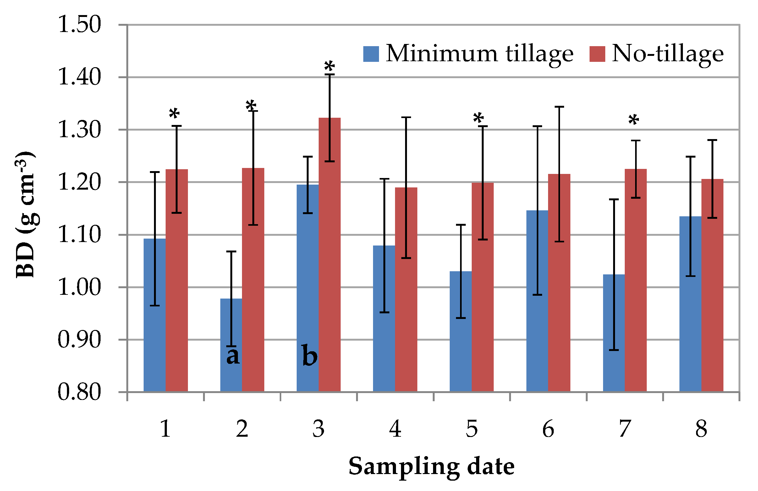
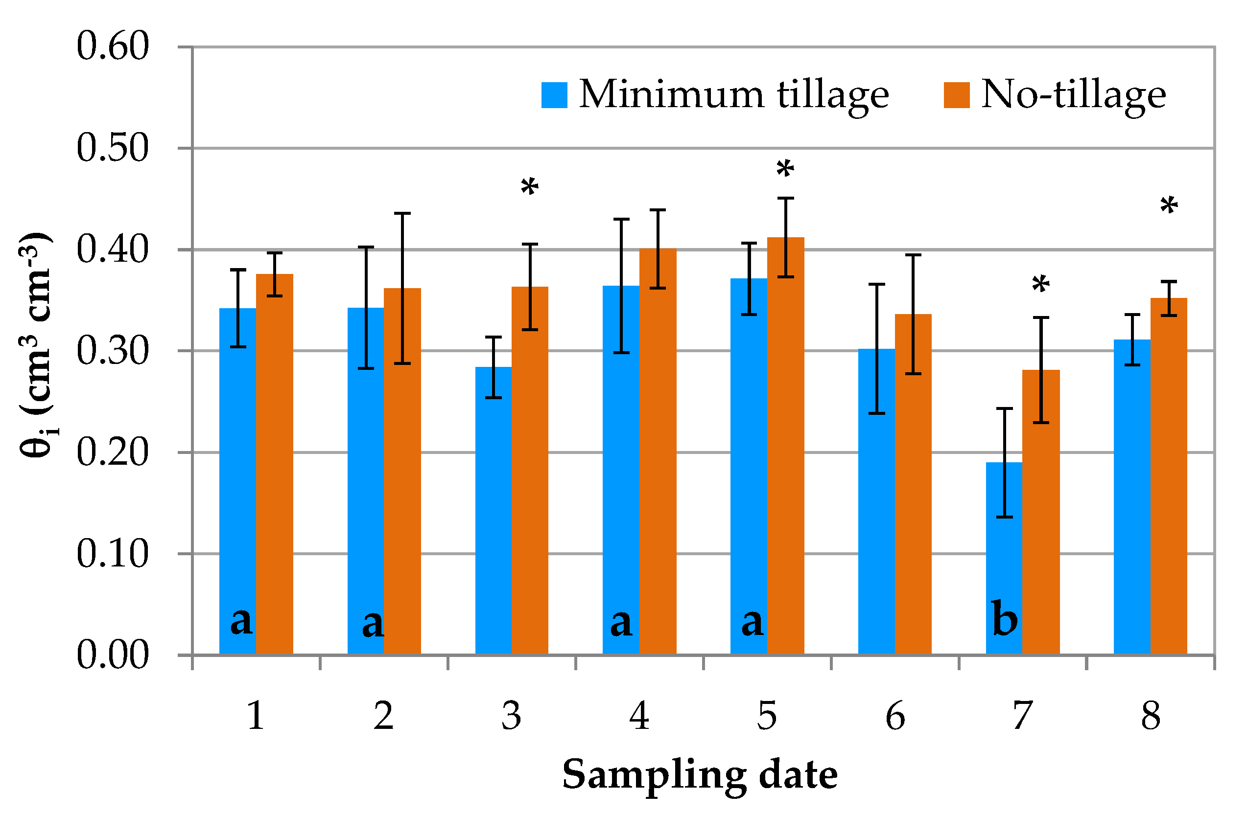
3.1. Temporal Variability of Soil Properties Using the SFH Technique

The results of soil bulk density (BD) and volumetric soil water content at the time of SFH experiments (θ_i) under MT and NT are reported in Figure 3 and Figure 4, respectively. Overall, higher BD values were observed under NT than MT, as, on average, they varied in the range (min–max) of 0.98–1.19 g cm⁻³ under MT and 1.19–1.32 g cm⁻³ under NT. On five of the eight sampling dates, BD values under NT were significantly higher than under MT (Figure 3). A lack of temporal variability was observed for BD because significant differences were identified only under MT between sampling dates 2 and 3 (i.e., between the beginning of May and July). Overall, detecting some discrepancies of BD values at the beginning of the crop cycle is quite expected as a result of the residual effects of the last soil tillage; however, a comparison with bulk densities of April 2016 suggests possible underestimation in May under MT due to unknown factors that make them difficult to assess. Soil water contents were higher under NT (0.28–0.41 cm³ cm⁻³) than under MT (0.19–0.37 cm³ cm⁻³) (Figure 4). Specifically, θ_i values showed significant differences between MT and NT on four dates (i.e., 3, 5, 7, and 8), namely between the end of spring and the beginning of autumn (Figure 4). Moreover, compared to BD, a relatively higher temporal variability was identified because the θ_i value of sampling date 7 was significantly lower than those of other dates, i.e., 1, 2, 4 and 5. This suggests that under MT/NT alters θ_i more than BD over time due to the different soil management.

Field saturated hydraulic conductivity (K_fs,SFH) changed over time within two or three orders of magnitude when the minimum–maximum interval or the geometric mean was considered, respectively (

Table 1. Minimum (Min), maximum (Max), geometric mean (GM), and associated geometric coefficient of variation (CV) of field saturated hydraulic conductivity (mm h⁻¹) carried out under MT and NT during each sampling date with the SFH technique.

Minimum Tillage (MT)
Sampling date	1	2	3	4	5	6	7	8
Min	3	2	1520	131	23	1617	258	930
Max	837	718	3800	1028	295	2606	2158	2349
GM	66 a *	45 a	2240 a	322 a	93 a	2210 a	799 a	1389 a
CV (%)	732	375	28	72	117	13	67	33
No-Tillage (NT)
Sampling date	1	2	3	4	5	6	7	8
Min	8	3	1074	33	195	801	182	529
Max	351	271	2050	384	659	1896	1476	2023
GM	81 b	28 b	1487 a	108 a	357 a	1474 a	590 b	1155 b
CV (%)	211	297	22	89	42	25	75	48

* For a given sampling date, mean values of soil management (i.e., MT and NT) followed by the same letter are not statistically different according to a two-tailed t-test (p = 0.05).

). K_fs,SFH was generally higher under MT than under NT (by a factor of 1.2–3.0); however, NT was higher on two occasions (sampling dates 1 and 5) by a factor of 1.2–3.8 (Table 1). According to a two-tailed t-test, the differences between MT and NT were significant in the first two and the last two sampling dates (Table 1). According to the THSD-test, which provides comparisons across all sampling dates (i.e., 28 possible combinations), the results of the temporal variability showed that K_fs,SFH was significantly different according to the different sampling dates in 60% of the considered cases (i.e., 17 of the 28 cases) under MT and 64% (18/28) under NT (

Table 2. Results of Tukey’s Honestly Significant Difference (THSD)-test (p = 0.05) on mean values of field saturated hydraulic conductivity measurements carried out with the SFH technique under minimum tillage (a) and no tillage (b) for each sampling date (from 1 to 8). Note that discrepancies in temporal variability between soil management are highlighted in yellow.

(a)

1

2

3

4

5

6

7

(b)

1

2

3

4

5

6

7

2

NS

2

NS

3

X

X

3

X

X

4

X

X

X

4

NS

X

X

5

NS

NS

X

NS

5

X

X

X

X

6

X

X

NS

X

X

6

X

X

NS

X

X

7

X

X

NS

NS

X

NS

7

X

X

NS

X

NS

NS

8

X

X

NS

X

X

NS

NS

8

X

X

NS

X

NS

NS

NS

NS = not significant difference; X = significant difference.

). This confirms a relatively high temporal variability of field saturated hydraulic conductivity. The temporal dynamics of K_fs,SFH between MT and NT were quite similar because the results of the THSD-test were simultaneously significant or not significant in 75% of the cases (i.e., 21 out of 28 cases) (Table 2). However, although θ_i values were generally comparable under MT and NT and their ratio was close to one (i.e., 0.9), discrepancies in K_fs values were detected according to the soil use, as only 3–5 sampling dates (2, 3, 6, 7, and 8) showed a ratio of K_fs,SFH values close to 1. A further deepening about the similarities among the aforementioned sampling dates (i.e., applying a cluster analysis) suggests three main groups (namely 4, 1 and 5, and all the remaining groups), but no link to the month of the year was found.

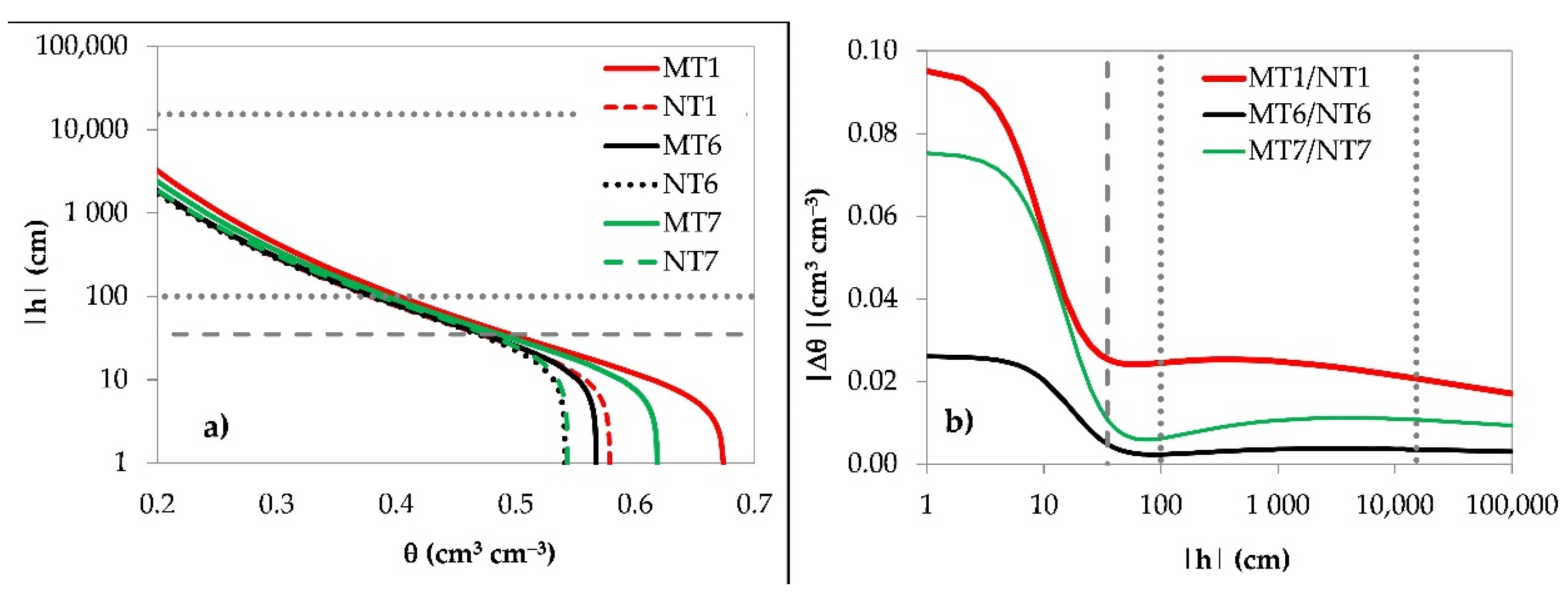
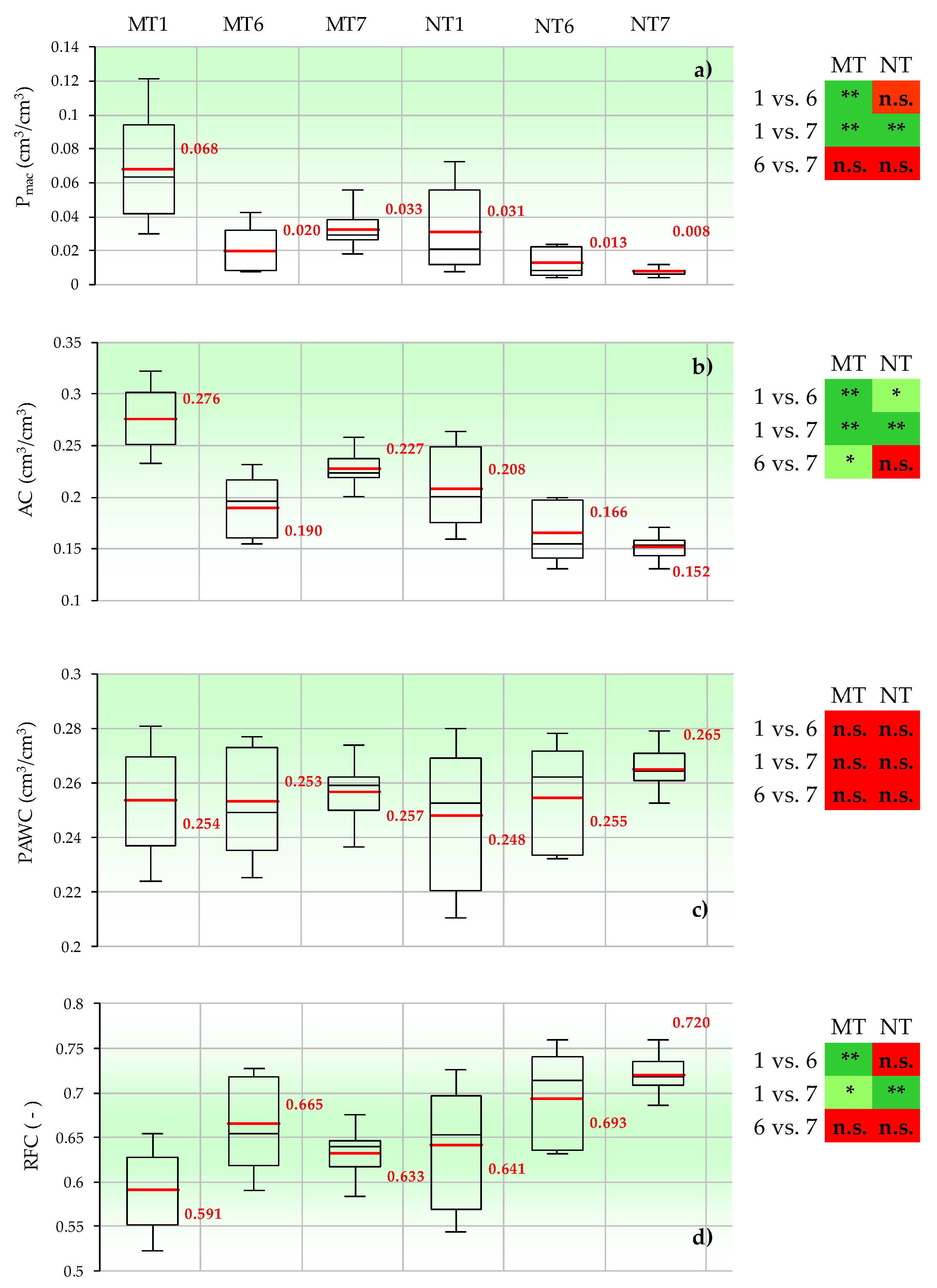
3.2. Temporal Variability of Soil Properties Using the BEST Procedure

Between the selected algorithms, only the BEST-intercept provided an adequate number of positive outcomes (i.e., 100% of the reps were analyzable and provided a complete soil hydraulic characterization), as the BEST-slope returned a K_fs,BEST estimation only in less than 20% (12/58) of the cases. The failures were due to the inability to correctly estimate the soil sorptivity, and negative estimations of K_fs,BEST were obtained. With the exception of two infiltration tests for which the two calculation algorithms provided discrepancies greater than one order of magnitude (i.e., a factor of 16 or 22), for ten of the twelve estimates obtained, K_fs,BEST differed at most by a factor of 3 or 4. Therefore, since only the BEST-intercept provided an adequate sample size, this algorithm was used to investigate the temporal variability of estimated soil properties and to establish the comparison in terms of K_fs between the BEST and SFH techniques.

The results of K_fs,BEST are reported in

Table 3. Minimum (Min), maximum (Max), geometric mean (GM), and associated geometric coefficient of variation (CV) of field saturated hydraulic conductivity (mm h⁻¹) carried out under MT and NT during each sampling date with the BEST-intercept.

Minimum Tillage (MT)
Sampling date	1	6	7
Min	202.9	105.0	99.5
Max	2512.2	1412.4	503.5
GM	1118.5 a,A *	507.7 a,B	176.9 a,B
CV (%)	77.7	146.4	53.8
No-Tillage (NT)
Sampling date	1	6	7
Min	16.9	18.8	56.5
Max	360.6	486.8	1906.0
GM	70.8 b,A	115.3 a,A	148.9 a,A
CV (%)	124.7	224.4	123.2

* For a given sampling date, mean values of alternative soil management types (i.e., MT and NT) followed by the same lowercase letter are not statistically different according to a two-tailed t-test (p = 0.05). For a given soil management type, mean values of different sampling dates (i.e., 1, 6, and 7) followed by the same capital letter are not statistically different according to a THSD-test (p = 0.05).

. Overall, relatively higher discrepancies between minimum and maximum values were detected under NT (within a factor of 4–34) than under MT (factor of 5–13); consequently, the associated variability was about double under NT (Table 3). Similarly to the results obtained by SFH, higher K_fs,BEST values were always detected, on average, under MT than NT, with differences equal to a factor of 15.8, 3.5, or 1.2 in the sampling dates 1, 6, and 7, respectively. According to a two-tailed t-test, the differences were significant only for sampling date 1. Moreover, due to the relatively high K_fs,BEST value for MT-1, temporal changes were detected only under MT (Table 3).

The BEST-derived soil water retentions are depicted in Figure 5a. Differences between MT and NT or between sampling dates were mainly located near to soil saturation, while they were relatively smaller in the unsaturated zone. This was because the BEST procedure considers a starting point of the water retention curve (i.e., the saturated soil water content) that depends on bulk density measured at the time of the experiment; also, in this area, the effect of soil structure estimated from Beerkan infiltration is higher. Consequently, differences in water retention between MT and NT decreased as soil pressure head increased, changing in the range of about 0.02–0.10 cm³ cm⁻³ at saturation and not exceeding 0.02 cm³ cm⁻³ between field capacity and wilting point (Figure 5b). For a given sampling date, a sensitivity analysis performed by running the BEST-intercept again with the same mean BD value for MT and NT (i.e., they differed only in the Beerkan infiltration) suggested that the effects of soil structure, as compared to soil texture, should be relevant (structure >> texture) until the field capacity; beyond this threshold, the effect of soil texture should become proportionally increasingly relevant (structure << texture). Furthermore, this suggests that the temporal variation in plant available water may have been negligible (Figure 5b).

The temporal variabilities of macroporosity (P_mac), air capacity (AC), plant available water capacity (PAWC), and relative field capacity (RFC) under MT and NT are shown in Figure 6. Overall, with the exception of PAWC, which was quite constant between sampling dates (about 0.25 cm³ cm⁻³), mean values of P_mac and AC varied in the ranges of 0.01–0.07 and 0.15–0.28 cm³ cm⁻³, respectively, whereas RFC was in the range of 0.59–0.72 (Figure 6). In addition, MT always showed the highest average soil porosity (i.e., lower RFC values indicate greater air capacity), whereas NT always showed the lowest one (similarly, higher RFC values indicate higher soil compaction). Among indicators and management of the soil considered in this investigation, relatively greater discrepancies between dates were generally detected for AC, whereas the smaller discrepancies were for PAWC. Moreover, depending on the considered soil management type, the results showed a temporal variability that was (i) equal between P_mac and RFC and (ii) opposite between AC and PAWC (Figure 6). Specifically, MT has always shown significant differences between sampling dates (7/12 or 58% cases), with the exception of PAWC (were never significant) or for P_mac and RFC between MT6 and MT7; NT showed significant differences in fewer cases (4/12 or 33% cases), always involving the first sampling date (Figure 6). Finally, according to the reference values of the literature [29,46], the mean values of soil indicators suggest a worsening of soil physical quality moving from the sampling dates 1 to 6 to 7. Regardless of statistical significance, however, this general trend over time (i.e., decreasing for P_mac and AC or increasing for RFC) was more evident under NT, since MT showed some inconsistencies.

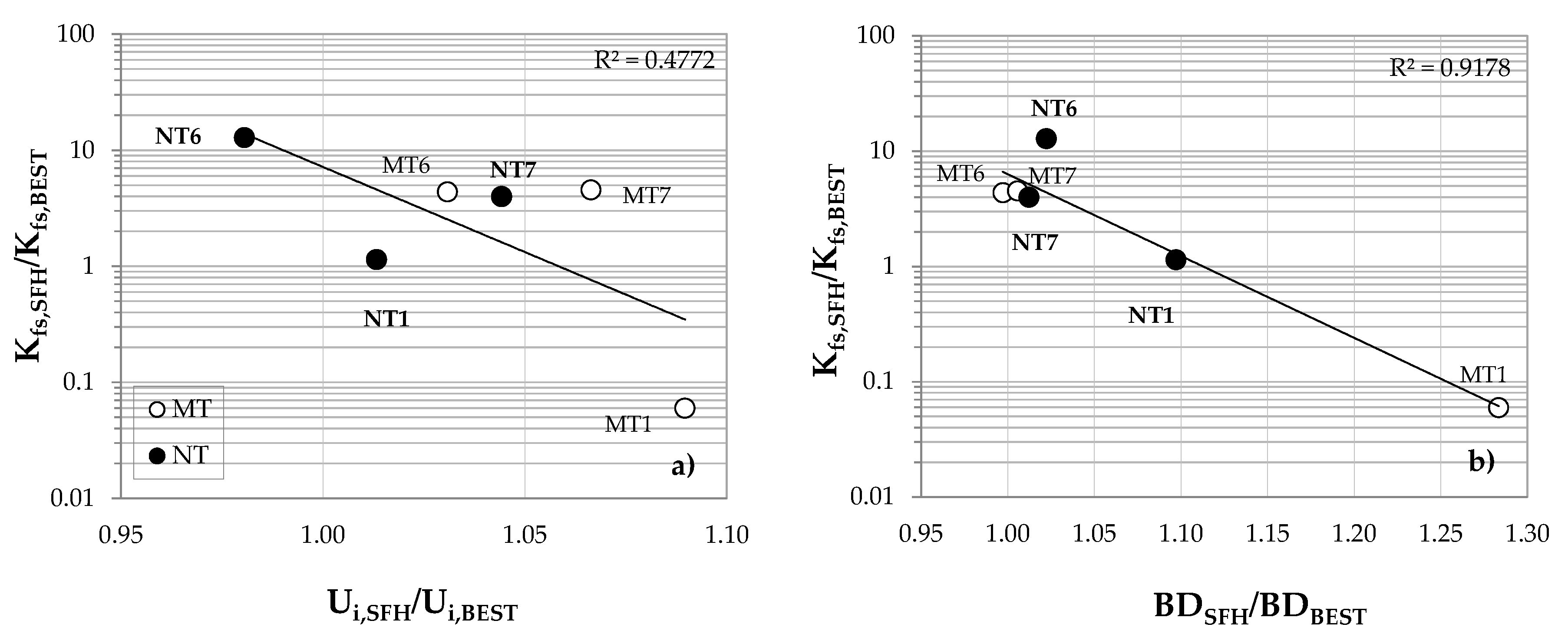
3.3. Comparison between the BEST and SFH Techniques

The results of saturated hydraulic conductivity obtained by SFH and BEST were described by the ratio K_fs,SFH/K_fs,BEST, which showed differences within a factor of 0.1–12.8 (Figure 7). Specifically, the aforementioned ratio was higher than one (K_fs,SFH > K_fs,BEST) for four out of six considered cases, while it was substantially lower than one or equal to one (K_fs,SFH ≤ K_fs,BEST) in the remaining cases. According to the latter, however, a ratio K_fs,SFH/K_fs,BEST of less than one was also found in a recent study [52], where clayey soils were also considered. Soil disturbance due to ring insertion or anisotropy of K_fs was suggested as the main cause for the underestimation obtained with SFH. For each sampling date, Figure 7 shows the ratio K_fs,SFH/K_fs,BEST as a function of the corresponding differences in gravimetric water content (Figure 7a), or as a function of the corresponding differences in soil bulk density (Figure 7b). Regardless of the moderate or strong correlation highlighted when U_i and BD were considered, findings from the linearized exponential function suggest that discrepancies in K_fs by a factor of 6 or 7 may be hypothesized between SFH and BEST when comparable BD or U_i values (i.e., relative difference equal to 1) were detected in the field (Figure 7). According to a t-test (p = 0.05), K_fs,SFH estimations were significantly higher, with the exception of NT1-MT1. This result could be expected because, although using stable cylinders can avoid possible underestimations due to the lack of soil compaction, K_fs,SFH overestimations cannot be excluded during the experiments due to possible preferential water flow (i.e., subsurface cracks, or along the edge of the cylinder). On the contrary, these measurement errors can be avoided by BEST because the ring is superficially inserted into the soil. Therefore, establishing comparisons between methods for field saturated hydraulic conductivity estimation is crucial for quantifying the accuracy of simplified methodologies. However, both methods provided the same information on the temporal variability of K_fs under MT, although discrepancies in the temporal variability evaluation were obtained under NT (i.e., a different result was obtained for two sampling dates, 1 vs. 6 or 7) (Table 3).

4. Discussion

Evaluating the temporal variability of the physical and hydraulic properties of the soil is crucial for crop modeling and, therefore, to assess the economic and environmental sustainability of specific soil management practices. In this investigation, the temporal variability of some physical and hydraulic properties was investigated over two years in a long-term agronomic experiment mainly aimed at comparing the effects of soil management practices, namely minimum tillage (MT) and no tillage (NT), by applying the SFH and BEST methods.

Temporal variability of K_fs detected by the SFH technique was comparable between MT and NT given that in 75% of the considered cases (i.e., 21/28 sampling dates), the same result (i.e., significant or not significant) was obtained (Table 2). On the other hand, when the temporal variability was investigated by BEST, a lack of significant differences was found (Table 3); this was partly due to a difference in the number of comparisons made (i.e., eight and three sampling dates, respectively, for SFH and BEST). However, when a homogeneous comparison between methods was made (considering the same sampling dates, i.e., 1, 6, and 7; Figure 2), similar results were always obtained for MT (i.e., same result in three out of three cases) while only in one out of three cases under NT, suggesting a higher temporal stability or a more difficult variability to capture under MT and NT, respectively. Therefore, the two methods could be not considered equivalent to study the temporal variability of K_fs when very heterogeneous soil conditions are sampled. However, a deeper analysis to better interpret the observed discrepancies under NT suggests a possible SFH overestimation on sampling dates 6 and 7 because: (i) The mean value of K_fs,SFH of sampling date 1 was significantly lower by a factor of 6 or 7; (ii) the ratio K_fs,SFH/K_fs,BEST was equal to a factor of 1, 13, and 4, respectively, on the three dates compared.

Although the compared methods (SFH and BEST) were very different for geometry of the water flow (1D or 3D, respectively) and therefore for the corresponding hydraulic modeling (transient or quasi-steady-state condition of the infiltration process), K_fs discrepancies between methods by a factor of 6 or 7 may be hypothesized when comparable BD or U_i values (i.e., a ratio approximately equal to one) were detected in the field. It is well known that transient methods could lead to higher K_fs estimates than stationary ones [26], and following a restrictive criterion, differences of K_fs obtained with alternative methods within a factor of 2 or 3 are considered negligible for practical purposes [37,53]. However, since slightly higher discrepancies were obtained in the present study, other factors should be taken into consideration to better understand SFH overestimation, including the (i) differences in the run duration, (ii) sampled soil volume, and (iii) possible preferential flow within the soil macropores or the soil water content at the time of experiment. In fact, although infiltration measurements were simultaneous, spatial variability should be considered as different according to the soil management type (i.e., due to probable local accumulations of organic matter), and Figure 7 confirms this hypothesis.

Studying the temporal variability of soil properties may also imply the accurate evaluation of some ancillary variables. Under MT, for example, a greater temporal variability of θ_i was detected, as compared with BD, only due to the low soil moisture values in the summer of 2017 (Figure 4).

Compared with SFH, the application of BEST could be considered more demanding in terms of experimental effort and specific skills for soil properties’ determination and data analysis. However, it allows the estimation of some main capacity-based soil indicators that are relevant for agronomic and environmental purposes and, therefore, the evaluation of their temporal changes over time. The comparison between the months of April 2016 and 2017 showed that there were no significant differences of P_mac, PAWC, and RFC under either MT or NT because they differed only in the air capacity of the soil (Figure 5). Moreover, since discrepancies in temporal variability were detected in only 3 out of 12 considered cases when all dates (and indicators) were considered, we may conclude that the two investigated soil management practices had a similar temporal variability, as shown by the capacity-based soil indicators estimated by BEST. This finding is important and not trivial, since it confirms several literature results emphasizing that long-term NT may show stable soil properties as compared with MT (among others, [31,32,54]). Results are also plausible because, in the three aforementioned cases (sampling date 1, P_mac and RFC; sampling date 3, AC), only MT changed over time, whereas NT was stable.

5. Conclusions

In this study, the temporal variability of some hydraulic soil properties was investigated over two years by applying the SFH and BEST techniques in a long-term field experiment for wheat cultivation under minimum tillage and no-tillage soil management.

Overall, the two soil management systems showed a relatively similar temporal variability of soil hydraulic properties (42% and 37%, respectively, under MT and NT), including bulk density, saturated hydraulic conductivity, macroporosity, air capacity, plant available water capacity, and relative field capacity. Although the two applied methods for K_fs estimation were basically different (among those to be highlighted, confined–unconfined or 1D–3D water flux, sampling volume), they provided similar information on the temporal variability of K_fs under MT, but not under NT, showing possible K_fs overestimations when SFH was used under no tillage. Therefore, although the two techniques appear to be equivalent in the MT system, further investigations are desirable to check these findings, and a greater number of dates compared would increase the reliability of the estimates.

However, when comparable soil conditions were sampled (i.e., water content and bulk density of the soil), the two methods differed by less than an order of magnitude (a factor of six or seven) with K_fs,SFH > K_fs,BEST. Therefore, if the main aim of the research is to intensively monitor the temporal variability of K_fs, the use of stable cylinders can be considered an inexpensive and quite accurate approach. Conversely, if hydraulic soil properties (water retention curve and hydraulic conductivity functions) are required, applying BEST is a way to estimate useful indicators to investigate, for example, the sustainability of soil management systems from a hydrological perspective. Although the latter technique is more complex than SFH, requiring certain extra measurements to run the available BEST calculation algorithms, their simultaneous use in the field can increase our confidence to quantify the impact of agronomic practices on soil physical properties.

In this long-term field experiment, characterized by 15 years of continuous soil management conducted with the methodological rigor typical of experimental farms, the BEST procedure allowed us to derive useful capacity-based indicators and confirmed a substantial equivalence between MT and NT for the fine-textured soil investigated.

References

1. Pirastru, M.; Bagarello, V.; Iovino, M.; Marrosu, R.; Castellini, M.; Giadrossich, F.; Niedda, M. Subsurface flow and large-scale lateral saturated soil hydraulic conductivity in a Mediterranean hillslope with contrasting land uses. J. Hydrol. Hydromech. 2017, 65, 297–306. [Google Scholar] [CrossRef] [Green Version]
2. Rallo, G.; Provenzano, G.; Castellini, M.; Sirera, A.P. Application of EMI and FDR sensors to assess the Fraction of Transpirable Soil Water over an olive grove. Water 2018, 10, 168. [Google Scholar] [CrossRef] [Green Version]
3. Ventrella, D.; Castellini, M.; Di Prima, S.; Garofalo, P.; Lassabatère, L. Assessment of the Physically-Based Hydrus-1D Model for Simulating the Water Fluxes of a Mediterranean Cropping System. Water 2019, 11, 1657. [Google Scholar] [CrossRef] [Green Version]
4. Crescimanno, G.; Morga, F.; Ventrella, D. Application of the SWAP model to predict impact of climate change on soil water balance in a Sicilian vineyard. Ital. J. Agron. 2011, 7, 116–123. [Google Scholar] [CrossRef] [Green Version]
5. Ventrella, D.; Charfeddine, M.; Giglio, L.; Castellini, M. Application of DSSAT models for an agronomic adaptation strategy under climate change in Southern Italy: Optimum sowing and transplanting time for winter durum wheat and tomato. Ital. J. Agron. 2012, 7, 109–115. [Google Scholar] [CrossRef]
6. Ventrella, D.; Giglio, L.; Charfeddine, M.; Lopez, R.; Castellini, M.; Sollitto, D.; Castrignanò, A.; Fornaro, F. Climate change impact on crop rotations of winter durum wheat and tomato in southern Italy: Yield analysis and soil fertility. Ital. J. Agron. 2012, 7, 100–108. [Google Scholar] [CrossRef] [Green Version]
7. Pirastru, M.; Niedda, M.; Castellini, M. Effects of maquis clearing on the properties of the soil and on the near-surface hydrological processes in a semi-arid Mediterranean environment. J. Agric. Eng. Res. 2014, 45, 176. [Google Scholar] [CrossRef]
8. Ferrara, R.M.; Mazza, G.; Muschitiello, C.; Castellini, M.; Stellacci, A.M.; Navarro, A.; Lagomarsino, A.; Vitti, C.; Rossi, R.; Rana, G. Short-term effects of conversion to no-tillage on respiration and chemical—Physical properties of the soil: A case study in a wheat cropping system in semi-dry environment. Ital. J. Agrometeorol. 2017, 47–58. [Google Scholar] [CrossRef]
9. Manici, L.M.; Castellini, M.; Caputo, F. Soil-inhabiting fungi can integrate soil physical indicators in multivariate analysis of Mediterranean agroecosystem dominated by old olive groves. Ecol. Indic. 2019, 106, 105490. [Google Scholar] [CrossRef]
10. Castellini, M.; Stellacci, A.M.; Mastrangelo, M.; Caputo, F.; Manici, L.M. Estimating the soil hydraulic functions of some olive orchards: Soil management implications for water saving in soils of Salento peninsula (southern Italy). Agronomy 2020, 10, 177. [Google Scholar] [CrossRef] [Green Version]
11. Di Prima, S.; Castellini, M.; AbouNajm, M.R.; Stewart, R.D.; Angulo-Jaramillo, R.; Winiarski, T.; Lassabatere, L. Experimental assessment of a new comprehensive model for single ring infiltration data. J. Hydrol. 2019, 573, 937–951. [Google Scholar] [CrossRef] [Green Version]
12. Bagarello, V.; Iovino, M.; Elrick, D.E. A simplified falling-head technique for rapid determination of field-saturated hydraulic conductivity. Soil Sci. Soc. Am. J. 2004, 68, 66–73. [Google Scholar] [CrossRef]
13. Keller, T.; Sutter, J.A.; Nisse, K.; Rydberg, T. Using field measurement of saturated soil hydraulic conductivity to detect low-yielding zones in three Swedish fields. Soil Till. Res. 2012, 124, 68–77. [Google Scholar] [CrossRef]
14. Biddoccu, M.; Ferraris, S.; Pitacco, A.; Cavallo, E. Temporal variability of soil management effects on soil hydrological properties, runoff and erosion at the field scale in a hillslope vineyard, North-West Italy. Soil Till. Res. 2017, 165, 46–58. [Google Scholar] [CrossRef] [Green Version]
15. Chyba, J.; Kroulik, M.; Kristof, K.; Misiewicz, P.A. The influence of agricultural traffic on soil infiltration rates. Agron. Res. 2017, 15, 664–673. [Google Scholar]
16. Azam, M.G.; Zoebisch, M.A.; Wickramarachchi, K.S.; Ranamukarachchi, S.L. Site-specific soil hydraulic quality index to describe the essential conditions for the optimum soil water regime. Can. J. Soil Sci. 2009, 89, 645–656. [Google Scholar] [CrossRef]
17. Cherubin, M.R.; Karlen, D.L.; Franco, A.L.C.; Tormena, C.A.; Cerri, C.E.P.; Davies, C.A.; Cerri, C.E.P. Soil physical quality response to sugarcane expansion in Brazil. Geoderma 2016, 267, 156–168. [Google Scholar] [CrossRef]
18. Erban, T.; Stehlik, M.; Sopko, B.; Markovič, M.; Seifrtova, M.; Halesova, T.; Kovaříček, P. The different behaviors of glyphosate and AMPA in compost-amended soil. Chemosphere 2018, 207, 78–83. [Google Scholar] [CrossRef]
19. Lassabatère, L.; Angulo-Jaramillo, R.; Soria Ugalde, J.M.; Cuenca, R.; Braud, I.; Haverkamp, R. Beerkan estimation of soil transfer parameters through infiltration experiments–BEST. Soil Sci. Soc. Am. J. 2006, 70, 521. [Google Scholar] [CrossRef]
20. Castellini, M.; Di Prima, S.; Iovino, M. An assessment of the BEST procedure to estimate the soil water retention curve: A comparison with the evaporation method. Geoderma 2018, 320, 82–94. [Google Scholar] [CrossRef]
21. Yang, J.; Xu, X.; Liu, M.; Xu, C.; Luo, W.; Song, T.; Du, H.; Kiely, G. Effects of Napier grass management on soil hydrologic functions in a karst landscape, southwestern China. Soil Till. Res. 2016, 157, 83–92. [Google Scholar] [CrossRef]
22. Yang, J.; Xu, X.; Liu, M.; Xu, C.; Zhang, Y.; Luo, W.; Zhang, R.; Li, Z.; Kiely, G. Effects of Grain for Green program on soil hydrologic functions in karst landscapes, southwestern China. Agric. Ecosyst. Environ. 2017, 247, 120–129. [Google Scholar] [CrossRef]
23. Gonzalez-Merchan, C.; Barraud, S.; Bedell, J.P. Influence of spontaneous vegetation in stormwater infiltration system clogging. Environ. Sci. Pollut. Res. 2014, 21, 5419–5426. [Google Scholar] [CrossRef]
24. Lozano-Baez, S.E.; Cooper, M.; de Barros Ferraz, S.F.; Ribeiro Rodrigues, R.; Lassabatere, L.; Castellini, M.; Di Prima, S. Assessing Water Infiltration and Soil Water Repellency in Brazilian Atlantic Forest Soils. Appl. Sci. 2020, 10, 1950. [Google Scholar] [CrossRef] [Green Version]
25. Di Prima, S.; Rodrigo-Comino, J.; Novara, A.; Iovino, M.; Pirastru, M.; Keesstra, S.; Cerdà, A. Soil Physical Quality of Citrus Orchards Under Tillage, Herbicide, and Organic Managements. Pedosphere 2018, 28, 463–477. [Google Scholar] [CrossRef] [Green Version]
26. Angulo-Jaramillo, R.; Bagarello, V.; Iovino, M.; Lassabatere, L. Infiltration Measurements for Soil Hydraulic Characterization; Springer International Publishing: Cham, Switzerland, 2016; ISBN 978-3-319-31786-1. [Google Scholar] [CrossRef] [Green Version]
27. Castellini, M.; Stellacci, A.M.; Tomaiuolo, M.; Barca, E. Spatial Variability of Soil Physical and Hydraulic Properties in a Durum Wheat Field: An Assessment by the BEST-Procedure. Water 2019, 11, 1434. [Google Scholar] [CrossRef] [Green Version]
28. Kreiselmeier, J.; Chandrasekhar, P.; Weninger, T.; Schwen, A.; Julich, S.; Feger, K.-H.; Schwärzel, K. Temporal variations of the hydraulic conductivity characteristic under conventional and conservation tillage. Geoderma 2020, 362, 114127. [Google Scholar] [CrossRef]
29. Castellini, M.; Stellacci, A.M.; Barca, E.; Iovino, M. Application of multivariate analysis techniques for selecting soil physical quality indicators: A case study in long-term field experiments in Apulia (southern Italy). Soil Sci. Soc. Am. J. 2019, 83, 707–720. [Google Scholar] [CrossRef] [Green Version]
30. Colecchia, S.A.; Rinaldi, M.; De Vita, P. Effects of tillage systems in durum wheat under rainfed Mediterranean conditions. Cereal Res. Commun. 2015, 43, 704–716. [Google Scholar] [CrossRef] [Green Version]
31. Castellini, M.; Fornaro, F.; Garofalo, P.; Giglio, L.; Rinaldi, M.; Ventrella, D.; Vitti, C.; Vonella, A.V. Effects of no-tillage and conventional tillage on physical and hydraulic properties of fine textured soils under winter wheat. Water 2019, 11, 484. [Google Scholar] [CrossRef] [Green Version]
32. Strudley, M.; Green, T.; Ascough, J.C., II. Tillage effects on soil hydraulic properties in space and time: State of the science. Soil Till. Res. 2008, 99, 4–48. [Google Scholar] [CrossRef]
33. Peterson, G.A.; Lyon, D.J.; Fenster, C.R. Valuing long-term field experiments: Quantifying the scientific contribution of a long-term tillage experiment. Soil Sci. Soc. Am. J. 2012, 76, 757–765. [Google Scholar] [CrossRef] [Green Version]
34. Körschens, M. The importance of long-term field experiments for soil science and environmental research—A review. Plant Soil Environ. 2006, 52, 1–8. [Google Scholar]
35. Philip, J.R. Falling head ponded infiltration. Water Resour. Res. 1992, 28, 2147–2148. [Google Scholar] [CrossRef]
36. Bagarello, V.; Baiamonte, G.; Castellini, M.; Di Prima, S.; Iovino, M. A comparison between the single ring pressure infiltrometer and simplified falling head techniques. Hydrol. Process. 2014, 28, 4843–4853. [Google Scholar] [CrossRef]
37. Elrick, D.E.; Reynolds, W.D. Methods for analyzing constant-head well permeameter data. Soil Sci. Soc. Am. J. 1992, 56, 320–323. [Google Scholar] [CrossRef]
38. Castellini, M.; Giglio, L.; Niedda, M.; Palumbo, A.D.; Ventrella, D. Impact of biochar addition on the physical and hydraulic properties of a clay soil. Soil Till. Res. 2015, 154, 1–13. [Google Scholar] [CrossRef]
39. Van Genuchten, M.T. A closed-form equation for predicting the hydraulic conductivity of unsaturated soils. Soil Sci. Soc. Am. J. 1980, 44, 892–898. [Google Scholar] [CrossRef] [Green Version]
40. Burdine, N.T. Relative permeability calculation from pore size distribution data. Petr. Trans. Am. Inst. Min. Metall. Eng. 1953, 198, 71–77. [Google Scholar] [CrossRef]
41. Brooks, R.H.; Corey, T. Hydraulic Properties of Porous Media; Hydrology Paper 3; Colorado State University: Fort Collins, CO, USA, 1964. [Google Scholar]
42. Haverkamp, R.; Debionne, S.; Viallet, P.; Angulo-Jaramillo, R.; de Condappa, D. Soil Properties and Moisture Movement in the Unsaturated Zone. In The Handbook of Groundwater Engineering; Delleur, J.W., Ed.; CRC Press: Boca Raton, FL, USA, 2006; pp. 1–59. [Google Scholar]
43. Haverkamp, R.; Ross, P.J.; Smettem, K.R.J.; Parlange, J.Y. Three-dimensional analysis of infiltration from the disc infiltrometer: 2. Physically based infiltration equation. Water Resour. Res. 1994, 30, 2931–2935. [Google Scholar] [CrossRef] [Green Version]
44. Yilmaz, D.; Lassabatère, L.; Angulo-Jaramillo, R.; Deneele, D.; Legret, M. Hydrodynamic characterization of basic oxygen furnace slag through an adapted BEST method. Vadose Zone J. 2010, 9, 107. [Google Scholar] [CrossRef]
45. Di Prima, S. Automatic Analysis of Multiple Beerkan Infiltration Experiments for Soil Hydraulic Characterization. In Proceedings of the 1st CIGR Inter-Regional Conference on Land and Water Challenges, Bari, Italy, 10–14 September 2013; p. 127. [Google Scholar] [CrossRef]
46. Reynolds, W.D.; Drury, C.F.; Tan, C.S.; Fox, C.A.; Yang, X.M. Use of indicators and pore volume-function characteristics to quantify soil physical quality. Geoderma 2009, 152, 252–263. [Google Scholar] [CrossRef]
47. Castellini, M.; Pirastru, M.; Niedda, M.; Ventrella, D. Comparing physical quality of tilled and no-tilled soils in an almond orchard in southern Italy. Ital. J. Agron. 2013, 8, 149–157. [Google Scholar] [CrossRef]
48. Zangiabadi, M.; Gorji, M.; Shorafa, M.; Khorasani, S.K.; Saadat, S. Effects of soil pore size distribution on plant available water and least limiting water range as soil physical quality indicators. Pedosphere 2020, 30, 253–262. [Google Scholar] [CrossRef]
49. Agnese, C.; Bagarello, V.; Baiamonte, G.; Iovino, M. Comparing physical quality of forest and pasture soils in a Sicilian watershed. Soil Sci. Soc. Am. J. 2011, 75, 1958–1970. [Google Scholar] [CrossRef]
50. Lee, D.M.; Elrick, D.E.; Reynolds, W.D.; Clothier, B.E. A comparison of three field methods for measuring saturated hydraulic conductivity. Can. J. Soil Sci. 1985, 65, 563–573. [Google Scholar] [CrossRef]
51. Bagarello, V.; Sgroi, A. Using the simplified falling head technique to detect temporal changes in field-saturated hydraulic conductivity at the surface of a sandy loam soil. Soil Till. Res. 2007, 94, 283–294. [Google Scholar] [CrossRef]
52. Bagarello, V.; Baiamonte, G.; Caia, C. Variability of near-surface saturated hydraulic conductivity for the clay soils of a small Sicilian basin. Geoderma 2019, 340, 133–145. [Google Scholar] [CrossRef]
53. Alagna, V.; Bagarello, V.; Di Prima, S.; Iovino, M. Determining hydraulic properties of a loam soil by alternative infiltrometer techniques. Hydrol. Processes 2016, 30, 263–275. [Google Scholar] [CrossRef] [Green Version]
54. Vogeler, I.; Rogasik, J.; Funder, U.; Panten, K.; Schnug, E. Effect of tillage systems and P-fertilization on soil physical and chemical properties, crop yield and nutrient uptake. Soil Till. Res. 2009, 103, 137–143. [Google Scholar] [CrossRef]
Figure 1. View of the experimental site for hydraulic property determination under minimum-tillage (MT) and no-tillage (NT) soil management (a); detail of the layer thickness of the wheat straw (NT) in November (b); detail of Beerkan infiltration experiments (c); detail of the simplified falling head (SFH) technique (d) in April.
Sustainability 12 05019 g001
Figure 2. Timeline of field measurements carried out under MT and NT using the SFH technique and Beerkan Estimation of Soil Transfer (BEST) procedure (eight and three sampling dates, respectively). At the bottom, the time intervals (days) between two successive SFH (a) and BEST (b) measurements are also reported inside the arrows.
Sustainability 12 05019 g002
Figure 3. Soil bulk density (BD) at the time of the SFH experiments. For a given sampling date, mean values of minimum tillage or no tillage marked with an asterisk were statistically different according to a t-test (p = 0.05). For a given soil management type, only values of sampling date marked with a different lowercase letter (i.e., ab) were statistically different according to Tukey’s Honestly Significant Difference (THSD)-test (p = 0.05).
Sustainability 12 05019 g003
Figure 4. Volumetric soil water content (θi) at the time of the SFH experiments. For a given sampling date, mean values of minimum tillage or no tillage marked with an asterisk were statistically different based on a t-test (p = 0.05). For a given soil management type, only values of sampling date marked with a different lowercase letter (i.e., ab) were statistically different based on a THSD-test (p = 0.05).
Sustainability 12 05019 g004
Figure 5. Soil water retention curves under minimum tillage and no tillage (MT and NT, respectively) in the three sampling dates considered (first, sixth, and seventh) (a), and corresponding differences in soil water retention (Δθ) as a function of soil pressure head (h) (b). Dotted lines represent θ values at field capacity and the permanent wilting point, and the dashed line represents an estimated mean threshold value corresponding to a mean value of bulk density between different soil management types.
Sustainability 12 05019 g005
Figure 6. Box plots of macroporosity (a), air capacity (b), plant available water capacity (c), and relative field capacity (d) carried out for selected sampling dates (1, 6, and 7) under minimum tillage (MT) and no tillage (NT). The thick red line within each box represents the mean value (the fine black line, the median); mean values are also reported in red. The gradation of white–green color indicates the progressive transition of soil indicators from poor (white) towards optimal (green) values. For a given soil management, inferences of the THSD-test between dates (i.e., x vs. y) are also summarized (* p < 0.05; ** p < 0.01; n.s. not significant).
Sustainability 12 05019 g006
Figure 7. Differences of field saturated hydraulic conductivity, Kfs, as a function of corresponding differences in gravimetric soil water content, Ui (a), and soil bulk density, BD (b), carried out with SFH and BEST (i.e., SFH/BEST). Units are given in: mm h−1, g g−1, and g cm−3, respectively for Kfs, Ui, and BD.
Sustainability 12 05019 g007