A Harris Hawks Optimization Based Single- and Multi-Objective Optimal Power Flow Considering Environmental Emission

Abstract

The electric sector is majorly concerned about the greenhouse and non-greenhouse gas emissions generated from both conventional and renewable energy sources, as this is becoming a major issue globally. Thus, the utilities must adhere to certain environmental guidelines for sustainable power generation. Therefore, this paper presents a novel nature-inspired and population-based Harris Hawks Optimization (HHO) methodology for controlling the emissions from thermal generating sources by solving single and multi-objective Optimal Power Flow (OPF) problems. The OPF is a non-linear, non-convex, constrained optimization problem that primarily aims to minimize the fitness function by satisfying the equality and inequality constraints of the system. The cooperative behavior and dynamic chasing patterns of hawks to pounce on escaping prey is modeled mathematically to minimize the objective function. In this paper, fuel cost, real power loss and environment emissions are regarded as single and multi-objective functions for optimal adjustments of power system control variables. The different conflicting framed multi-objective functions have been solved using weighted sums using a no-preference method. The presented method is coded using MATLAB software and an IEEE (Institute of Electrical and Electronics Engineers) 30-bus. The system was used to demonstrate the effectiveness of selective objectives. The obtained results are compared with the other Artificial Intelligence (AI) techniques such as the Whale Optimization Algorithm (WOA), the Salp Swarm Algorithm (SSA), Moth Flame (MF) and Glow Warm Optimization (GWO). Additionally, the study on placement of Distributed Generation (DG) reveals that the system losses and emissions are reduced by an amount of 9.8355% and 26.2%, respectively.

1. Introduction

Optimal Power Flow (OPF) is one of the significant tools used over decades to date in energy management systems for reliable operation and proper planning of modern power systems. This problem is a non-linear, non-convex, and multi-dimensional optimization problem with control variables such as voltage magnitude and real power generation as continuous variables, and transformer tap ratios and shunt capacitor as discrete variables [1,2,3,4]. These variables are adjusted to operate the system efficiently and economically for continuous change in the load demand. Thus, the aim of OPF is to optimize the certain selective objectives of the system such as fuel cost, real and reactive power loss, voltage stability enhancement, and environmental emissions, ensuring the equality and inequality constraints [5]. Numerous classical and intelligence-based methods were used to solve the OPF problem and are portrayed in Figure 1. Through rigorous analysis, it is observed that the conventional mathematical methods such as the gradient-based approach, the Newton method, the interior point method, and linear, non-linear, quadratic, and mixed integer programming have been successfully used to solve OPF problem [6,7,8,9,10,11,12]. These methods give the optimal results but fail at local minima, if the initial point is not assumed close to the solution. In addition, the quality of solutions highly degrades as the number of control variables increases. Further, the complexity of the problem is very high because of the number of non-linear constraints of the system [5,13]. To cater this problem, researchers for the last few decades use non-gradient, non-deterministic, and highly flexible meta-heuristic-based techniques to obtain the solution for OPF without trapping into local minima due to the advancement in computer technologies [1].

To date, the various meta-heuristic methods that have been used to solve OPF are portrayed in [14,15,16,17,18,19,20,21,22,23,24,25,26,27,28,29]. Generally, the meta-heuristic approaches are categorized into four major classes:

Evolutionary, swarm intelligence, physics and human-based algorithms [30]: The evolutionary algorithms (EA) are based on evolutionary principles that exist in nature such as selection, cross-over and mutation. The most well-known methods are the Genetic Algorithm (GA), evolution strategy, Differential Evolution (DE) and biogeography-based optimizations. All of these techniques are heuristic and initiated with random solutions, and the solution is updated by evaluating the fitness functions. On the other hand, the Swarm Intelligence (SI) techniques mimic creatures in nature and are very popular meta-heuristic optimization methods. SI-based methods include particle swarm, artificial bee colony [31], firefly algorithm [32], chaotic krill heard [33], backtracking search algorithm [34], efficient evolutionary algorithm [35], faster evolutionary algorithm [36], group search algorithm [37], differential evolution algorithm [38], multi-hive bee foraging algorithm [39], etc. Moreover, the affine arithmetic method [40], the knowledge-based framework human learning method [41], and linear compression methods [42] were used to solve optimal power flow problems. These methods are self-organizing systems that can operate based on mathematical equations developed using a set of rules depicting the behavior of a swarm to give the stable solution after convergence. On the flipside, the physics-based intelligence approaches imitate the physical laws that govern the evolution of the universe—the law of gravity, the electromagnetism law, the force of attraction, and so on. The various algorithms based on physics include the Gravitational Search Algorithm (GSA), Central Force Optimization (CFO), Big Bang-Big Crunch, galaxy-based, and magnetic optimization, etc.; these techniques are reviewed and presented in [43]. The human-based optimization techniques are developed based on human traits and their invention; some of these methods are teaching learning, group search, harmony, and tabu search used to minimize real world complex problems. The aforementioned various intelligence-based methods are applied to many engineering problems and give effective solutions to some problems, but fail for other kinds of problems.

Regardless of the different methods, the common features that exist are the exploration and exploitation characteristics. In the former phase, the algorithm should utilize its randomized parameters as much as possible and find the feature space through its local search ability in the search regions. In the later phase of exploitation, the algorithm tries to find a global optimal solution by intensifying the search process in a local region instead of an entire region of search space. A well-optimized technique should posses the following characteristics for avoiding the possibility of convergence to local optima [22,44,45]. In relation to the previously published work, it is inferred that most of the study focused on single objective optimization, and in particular, the minimization of either power loss or generating cost. However, recently the increase in the environmental pollutant gases such as ${\mathrm{CO}}_2,{ \mathrm{SO}}_2,{ \mathrm{and} \mathrm{NO}}_2$ emissions during power generation and its serious impact on the environment has gained more attention. The US clean air act amendments of1990 directed utility companies to produce energy in keeping the pollution at the minimum level in association with other power system constraints [45]. In view of this, different methods such as the hybrid dragonfly and particle swarm optimization algorithm, penalty function methods and the improved strength pare to evolutionary algorithm have been implemented to curtail this harmful emission, like implementing Carbon Capture and Sequestration (CCS) technology [15,46,47].

Furthermore, real world design and optimization problems always involve more than one conflicting objectives. Thus, Multi-Objective (MO) optimization has earned huge attention among researchers [26]. To handle such opponent objectives simultaneously, AI techniques have transferred into multi-objective optimization by modifying it with the aid of various classical methods. To solve this MO function, numerous methods have been presented in [48,49,50], such as the penalty function method, weighted sum method, ϵ-constant method, non-dominated sorting genetic algorithm-based approach, strength Pareto evolutionary algorithm, etc. Despite of having a variety of intelligence algorithms, none of these methods can assure the consistency of an optimal solution for solving all of the objectives. This incentivizes the researcher to develop many new nature-inspired algorithms day by day, which possess the traits of exploration and exploitation that can solve all the real-time optimization problems without reaching divergence or local convergence [15,51]. In this paper, a maiden attempt has been made to apply a Harris Hawks-based Optimization (HHO) approach for OPF. HHO is a nature-inspired optimization technique proposed by Heidari [49] that competes with other optimization methods portrayed in the literature with its cooperative behaviors to attack the hunting prey. Moreover, the hunting and escaping strategies are analyzed through mathematical calculations to reach a global solution with effective computational time. The main contributions of this work areas follows:

• To optimize the fuel cost, power loss, and emission cost of the system by solving single- and multi-objective OPFs using the HHO algorithm;
• To handle the equality and inequality constraints such as voltage magnitude, transformer tap ratio, and real and reactive power constraints of the generator while optimizing the various objectives;
• To optimally place the Distributed Generation (DG) based on a real power sensitivity index for minimizing the loss and emission;
• To statistically compare the results obtained with other well-known nature-inspired methods such as SSA, WOA, MF, and GWO.

The remainder of the paper is organized as follows: Section 2 deals with the OPF problem formulation, which contains single and multi-objective problem formations mathematically, including equality and inequality constraints. Section 3 presents an extended introduction of the proposed intelligence-based HHO algorithms with numerical presentation and with a dynamic levy flight strategy. The comparison of numerical results and discussion among well-known other nature-inspired methods of optimization and proposed approaches are portrayed in Section 4. Section 5 describes the comparative analysis of the proposed method with the literature work. Finally, Section 6 presents the conclusion and the future scope of the work.

2. OPF Formulation

This section describes the various competing objective functions to be minimized as follows.

2.1. Total Fuel Cost Minimization (TFC)

The TFC is considered as the prime objective function for the OPF problem, which is the quadratic function of real power generations of generators. It can be mathematically defined as [13,44]:

$${\mathrm{f}}_1={\displaystyle \sum _{\mathrm{i}=1}^{\mathrm{NG}}{\mathrm{a}}_{\mathrm{i}}}+{\mathrm{b}}_{\mathrm{i}}{\mathrm{P}}_{\mathrm{Gi}}+{\mathrm{c}}_{\mathrm{i}}{\mathrm{P}}_{\mathrm{Gi}}{}^2\$/\mathrm{h}\hspace{1em}\hspace{1em}\mathrm{i}=1, 2, \dots , {\mathrm{N}}_{\mathrm{G}}$$

(1)

where P_Gi is the total power generation in MW, and a_i, b_i, and c_i denote the cost co-efficient of a specific generator, while N_G is the total number of generators in the system.

2.2. Active Power Loss Minimization (APL)

The APL can be optimized by tuning the controlling parameters by satisfying power flow constraints properly and can be described as [5,44]:

$${\mathrm{f}}_2={\displaystyle \sum _{\mathrm{i}=1}^{\mathrm{NL}}{\mathrm{g}}_{\mathrm{i}}}[{\mathrm{V}}_{\mathrm{k}}{}^2+{\mathrm{V}}_{\mathrm{m}}{}^2-2{\mathrm{V}}_{\mathrm{k}}{\mathrm{V}}_{\mathrm{m}}\cos ({\mathsf{\delta }}_{\mathrm{k}}-{\mathsf{\delta }}_{\mathrm{m}})]\mathrm{MW} \mathrm{i}=1, \dots , {\mathrm{N}}_{\mathrm{L}}$$

(2)

where g_i is the transfer conductance, V_k and V_m represent the voltage magnitude from and to the bus, δ_k and δ_m depict the phase angle, and N_L is the total number of transmission lines of the system.

2.3. Total Emission Cost Minimization (TEC)

Owing to an increase in the energy demand, the utilities need to generate a surplus large amount of power to meet the load demand. The only stable source of generation is thermal generating units compared to other units of generation. These generating units produce a byproduct in addition to the electrical power, such as CO₂, SO₂, NO₂, and so on, which contaminate the environment and increases the air pollution. Therefore, the prime purpose of this function is to mitigate the emission of toxic substances to the air by optimizing the corresponding control variables of the power system. The TEC of power generating units can be mathematically formulated as follows [15,44]:

$${\mathrm{f}}_3={\displaystyle \sum _{\mathrm{i}=1}^{\mathrm{NG}}{\mathsf{\alpha }}_{\mathrm{i}}+{\mathsf{\beta }}_{\mathrm{i}}}{\mathrm{P}}_{\mathrm{G}\mathrm{i}}+{\mathsf{\gamma }}_{\mathrm{i}}{\mathrm{P}}_{\mathrm{G}\mathrm{i}}{}^2+{\mathsf{\zeta }}_{\mathrm{i}}\exp ({\mathsf{\lambda }}_{\mathrm{i}}{\mathrm{P}}_{\mathrm{G}\mathrm{i}})\mathrm{ton}/\mathrm{h}$$

(3)

whereα, β, γ, ε, and λ are the environmental emission coefficients, and P_Gi is the real power generation.

These objective functions are regarded as single-objective OPF problems and their solutions are obtained using the proposed HHO techniques. In the actual operation of a power system, there might be a situation in which to optimize more than one parameter. In this case, the multi-objective optimization plays a major role in minimizing more than one conflicting objective simultaneously by fulfilling the constraints of the system. Many literature works portrayed in the introduction attempted to solve the single-objective optimization for OPF applications. Only a few researchers solved the multi-objective problem, and sometimes they failed to claim the effectiveness of their proposed method for both single and multi-objective problems. In this work, an attempt has been made to solve both single and multi-objectives concurrently, and the performance of the proposed HHO method is presented. In general, the multi-objective function can be expressed as is defined bellow:

$$\begin{array}{c}\mathrm{Minimize},{\mathrm{J}}_{\mathrm{m}}(\mathrm{x},\mathrm{u})={\displaystyle \sum _{\mathrm{m}=1}^{\mathrm{N}}{\mathrm{w}}_{\mathrm{m}}}{\mathrm{f}}_{\mathrm{m}}(\mathrm{x},\mathrm{u})\mathrm{m}=1, 2, \dots , \mathrm{N} \\ ={\mathrm{w}}_1{\mathrm{f}}_1+{\mathrm{w}}_2{\mathrm{f}}_2+{\mathrm{w}}_3{\mathrm{f}}_3 \dots ,+{\mathrm{w}}_{\mathrm{m}}{\mathrm{f}}_{\mathrm{m}}\end{array}$$

(4)

subjected to:

g_j (x, u) = 0 j = 1, 2, 3, …, N

(5)

h_k (x, u) ≤ 0 k = 1, 2, 3, …, N

(6)

where J is the multi-objective function with m number of functions, f represents the individual objective function, and w is the scalar weight multiplied with each objectives whose values lies in the range of 0 to 1. It is worth mentioning that the total sum of weight is equal to one. The multi-objective function in this work is solved using the no-preference weighted sum approach. In this approach, no prime significance is given to any of the objectives, but a heuristic is used to obtain the single optimal solution. However, it is also important to notice that this method does not attempt to find multiple Pareto-optimal solutions [50,52]. The various conflicting multi-objectives framed are as follows.

2.4. TFC and APL Minimization

The most conflicting objectives called TFC and APL are considered as the selective objectives to be optimized simultaneously. The optimization function can be defined as:

f₄ = w₁ × f₁ + w₂ × f₂.

(7)

2.5. TFC and TEC Reduction

The TFC and TEC together have been regarded as objective functions to be optimized and which are expressed as:

f₅ = w₁ × f₁ + w₂ × f₃.

(8)

2.6. APL and TEC Minimization

In this step, the APL and environmental emissions have been considered simultaneously for the optimization of selective objectives, which is formulated as follows:

f₆ = w₁ × f₂ + w₂ × f₃.

(9)

2.7. TFC, APL, and TEC Minimization

In this fragment, all of the objectives have been considered simultaneously for optimization, which is defined as:

f₇ = w₁ × f₁ + w₂ × f₂ + w₃ × f₃.

(10)

The equality and inequality constraints of the power system are as follows [5,45].

2.7.1. System Equality Constraints:

The aforementioned objective functions are optimized subjected to these constraints, which are defined as follows:

P_i (V, δ) − P_Gi + P_Di = 0 (i = 1, 2, 3, …, N)

(11)

Q_i (V, δ) − Q_Gi+ Q_Di = 0 (i = 1, 2, 3, …, N)

(12)

where P_i (V, δ) and Q_i (V, δ) are the power flow equations and can be defined as

$${\mathrm{P}}_{\mathrm{i}}(\mathrm{V},\mathsf{\delta })={\mathrm{V}}_{\mathrm{i}}{\displaystyle \sum _{\mathrm{j}=1}^{\mathrm{n}}{\mathrm{V}}_{\mathrm{j}}}({\mathrm{H}}_{\mathrm{ij}}\cos ({\mathsf{\delta }}_{\mathrm{i}}-{\mathsf{\delta }}_{\mathrm{j}})+{\mathrm{M}}_{\mathrm{ij}}\mathrm{s}\mathrm{i}\mathrm{n}({\mathsf{\delta }}_{\mathrm{i}}-{\mathsf{\delta }}_{\mathrm{j}})$$

(13)

$${\mathrm{Q}}_{\mathrm{i}}(\mathrm{V},\mathsf{\delta })={\mathrm{V}}_{\mathrm{i}}{\displaystyle \sum _{\mathrm{j}=1}^{\mathrm{n}}{\mathrm{V}}_{\mathrm{j}}}({\mathrm{H}}_{\mathrm{ij}}\mathrm{s}\mathrm{i}\mathrm{n}({\mathsf{\delta }}_{\mathrm{i}}-{\mathsf{\delta }}_{\mathrm{j}})-{\mathrm{M}}_{\mathrm{ij}}\cos ({\mathsf{\delta }}_{\mathrm{i}}-{\mathsf{\delta }}_{\mathrm{j}})$$

(14)

$${\displaystyle \sum _{\mathrm{i}=1}^{\mathrm{NG}}{\mathrm{P}}_{\mathrm{Gi}}={\mathrm{P}}_{\mathrm{Di}}}+{\mathrm{P}}_{\mathrm{loss}}$$

(15)

where N_G is the number of generator bus, N represent the total number of bus, P_i depicts the active power injection, Q_i denotes the reactive power injection, P_Di represent the active load, Q_Di is the reactive power load, P_Gi is the active power generation, Q_Gi is the reactive power generation, V is the voltage magnitude, and δ is the phase angle; the admittance matrix is defined as Y_ij = H_ij + jM_ij and i and j are the from and to buses, while P_loss is the active power loss.

2.7.2. System Inequality Constraints

• Generator constraints:

The real power, reactive power, and voltage constraints of generating units are:

P_Gimin ≤ P_Gi ≤ P_Gimax (i = 1, 2, 3, …, N_G)

(16)

Q_Gimin ≤ Q_Gi ≤ Q_Gimax (i = 1, 2, 3, …, N_G)

(17)

V_imin ≤ V_i ≤ V_imax (i = 1, 2, 3, …, N_G)

(18)

• Transformer constraints:

The lower and upper boundaries of the transformer tap settings can be represented by:

T_imin ≤ T_i ≤ T_imax (i = 1, 2, 3, …, N_T)

(19)

• Shunt compensator VAR constraints:

The switchable shunt compensation can be designated to operate within the limit of as follows:

Q_imin ≤ Q_i ≤ Q_imax (i = 1, 2, 3, …, N_G)

(20)

• Security constraints:

In addition, to equality and inequality constraints, for the system to be healthy the voltage at the load buses should be within the range of V_Limin to V_Limax as follows:

V_Limin ≤ V_Li ≤ V_Limax (i = 1, 2, 3, …, N)

(21)

S_Limin ≤ S_Li ≤ S_Limax (i = 1, 2, 3, …, N)

(22)

2.8. Sensitivity Indexfor Placementof DG

The active power loss sensitivity is considered the prime objective for placement of distribution generation (DG) in the system. The power loss of the system is defined as [53]:

$${\mathrm{P}}_{\mathrm{losses}}={{\displaystyle \sum }}_{\mathrm{i}=1}^{\mathrm{N}}{{\displaystyle \sum }}_{\begin{array}{c}\mathrm{i}=1\\ \mathrm{j}\ne 1\end{array}}^{\mathrm{N}}\frac{{\mathrm{G}}_{\mathrm{ij}}}{2}\left[\left|{\mathrm{V}}_{\mathrm{i}}^2\right|+\left|{\mathrm{V}}_{\mathrm{j}}^2\right|-2\left|{\mathrm{V}}_{\mathrm{i}}\right|\left|{\mathrm{V}}_{\mathrm{j}}\right|\cos \left({\mathsf{\delta }}_{\mathrm{i}}-{\mathsf{\delta }}_{\mathrm{j}}\right)\right].$$

(23)

The real and reactive power sensitivity indices for each load bus can be calculated as:

$$\left[\begin{array}{c}\frac{\partial {\mathrm{P}}_{\mathrm{losses}}}{\partial {\mathrm{P}}_{\mathrm{i}}}\\ \frac{\partial {\mathrm{P}}_{\mathrm{losses}}}{\partial {\mathrm{Q}}_{\mathrm{h}}}\end{array}\right]={\left[\mathrm{Jac}\right]}^{-1}\left[\begin{array}{c}\frac{\partial {\mathrm{P}}_{\mathrm{losses}}}{\partial {\mathsf{\delta }}_{\mathrm{i}}}\\ \frac{\partial {\mathrm{P}}_{\mathrm{losses}}}{\partial {\mathrm{V}}_{\mathrm{h}}}\end{array}\right]$$

(24)

where Jac is the Jacobian matrix, ∂P_loss/∂P_i and ∂P_loss/∂Q_h represent the variation in active and reactive power loss at the ith and hth bus, respectively. In this work, the real power loss sensitivity index is considered for the placement of DG and it is obtained by solving the above equation (24) resulted in as follows:

$$\frac{\partial {\mathrm{P}}_{\mathrm{losses}}}{\partial {\mathrm{P}}_{\mathrm{i}}}=2{{\displaystyle \sum }}_{\begin{array}{c}\mathrm{j}=1\\ \mathrm{j}\ne 1\end{array}}^{\mathrm{N}}{\mathrm{G}}_{\mathrm{ij}}\left[\left|{\mathrm{V}}_{\mathrm{i}}\right|\left|{\mathrm{V}}_{\mathrm{j}}\right|\sin \left({\mathsf{\delta }}_{\mathrm{i}}-{\mathsf{\delta }}_{\mathrm{j}}\right)\right].$$

(25)

The higher values of the index indicate the maximum power loss and the lower value depicts the minimum loss of the bus. For optimal placement of DG in the system, the bus with a higher of value of ∂P_loss/∂P_i is considered as a candidate bus for location.

3. Application of HHO to the OPF Problem

The Harris hawk is one of the most intelligent and distinguished predator birds in nature that demonstrates distinctive collective chasing capabilities in tracing, encircling, flushing out, and capturing the potential animal (rabbit) in a group for its food. Here, the initial population is assumed as a group of hawks that try to chase the targeted rabbit (solution of the optimization problem) from different directions by using seven killing strategies or a surprise pounce. Initially, the leader hawk tries to attack the prey; if it fails to grab the animal because of the dynamic nature and escaping behavior of the prey, the switching tactics are followed, so that the other party members (hawks in the group) will hit the escaped prey until seized. The main advantage of this collaborative tactic is that the birds can pursue the pointed rabbit by means of puzzling and exhaustion of the escaping prey. In HHO, the candidate solutions are the Harris Hawks and the optimal/global solution is the intended prey. Thus, HHO exhibits the exploratory and exploitative phases and are explained in Figure 2 and below [49].

Step1—Exploration phase: Harris hawks perch randomly and wait in some locations, observe and monitor to attack the prey. The leader hawks perch based on position of family members and prey. This is described in the form of a mathematical equation for changing in distance (q) between the hawks and prey as follows:

$$\mathrm{X}(\mathrm{i}+1)=\{\begin{array}{cc}{\mathrm{X}}_{\mathrm{rand}}(\mathrm{i})-{\mathrm{r}}_{{}^1}{\mathrm{X}}_{\mathrm{rand}}(\mathrm{t})-2{\mathrm{r}}_2\mathrm{X}(\mathrm{i})\hfill & \mathrm{q}\ge 0.5\hfill \\ {\mathrm{X}}_{\mathrm{r}}(\mathrm{i})-{\mathrm{X}}_{\mathrm{m}}(\mathrm{i})-{\mathrm{r}}_3(\mathrm{LB}+{\mathrm{r}}_4(\mathrm{UB}-\mathrm{LB})\hfill & \mathrm{q}<0.5\hfill \end{array}$$

(26)

where X(t+1) is the updating vector of the Hawk’s position atthei+1 iteration, X_r(t) is the position of the prey, X(t)is the position vector of the hawks at the ith iteration, r₁, r₂, r₃, r₄, and q are random numbers in the range of (0,1), UB and LB are the Upper and Lower Bounds of variables, and X_rand (t) and X_m(t)are the initial population assumed randomly.

The average position of each hawk is defined as:

$${\mathrm{X}}_{\mathrm{i}+1}(\mathrm{t})=\frac{1}{\mathrm{N}}{\displaystyle \sum _{\mathrm{i}=1}^{\mathrm{N}}{\mathrm{X}}_{\mathrm{i}}}(\mathrm{t})$$

(27)

where X_i(t) is the current position of hawks, X_i+1(t) is the updating position vector, and the total number of hawks is represented by N.

Step2: During the exploration phase, the hawks try to find and hit the prey. Due to this there is considerable change in the energy (E) of the prey and it is given by:

$$\mathrm{Escaping} \mathrm{Energy}, \mathrm{E}=2{\mathrm{E}}_0(1-\frac{\mathrm{t}}{\mathrm{T}})$$

(28)

where T is the maximum iteration count, t is the current iteration, and the initial energy (${\mathrm{E}}_0)$ randomly changes between (−1 to 1) at every iteration. E ≥ 1 indicates the leaping behavior of the prey and the hawks search for prey in other location, E < 1 indicates that the prey becomes exhausted and the hawk intensifies its attack by a surprise pounce that makes the solution to the exploitation phase.

Step3—Exploitation phase: At this stage, the switching tactics follow to attack the prey. The prey always tends to escape from hawks, and the chance of escaping of the prey is illustrated as r. When r < 0.5 the prey is successfully escaping, and on the flipside when r ≥ 0.5 the chance of escaping is unsuccessful. At any rate, the hawks will attack the prey and will be either successful or not through a soft or hard siege. If the prey escaped when (r ≥ 0.5) and |E| < 0.5 then a hard siege takes place. On the other hand, if (r ≥ 0.5) and |E| ≥ 0.5, then a soft siege occurs. Here, r is the chance of the prey escaping. This can be modeled in mathematical form as follows.

Step4—Soft siege: Here, the rabbit possesses energy and tries to escape by jumping and the hawks surround it softly, which is modeled as

X(t + 1) = ∆X(t) − E|JX_rabbit(t) − X(t)|

(29)

∆X(t) = X_rabbit(t) − X(t).

(30)

The random jump of the rabbit is given by J = 2(1 − r₅),where ∆X(t) is the difference between the position vectors of consecutive iteration and r5 is the random number that lies in the range of (0,1).

Step5—Hard siege: In this case, the prey is fully exhausted and the hawks encircle it hardly and perform the surprise pounce. The positions are updated using (28) as given by

X(t + 1) = X_rabbit(t) − E|∆X(t)|.

(31)

Step6—Soft siege with continuous rapid dives:

The rabbit still possesses the energy and tries to escape, and this is represented as |E| ≥ 0.5 and r < 0.5, and a further soft siege is required before the surprise pounce by the hawks. This step is more intelligent than the previous case. Here the Levy flight (LF) concept was introduced for progressive rapid dives of hawks to perform a soft siege and the next move of the prey is evaluated by the hawks using the following equation:

Y = X_rabbit (t) − E|JX_rabbit (t) − X(t)|.

(32)

Despite several attempts, the hawks compare each of their movements with the previous dive, to determine if it was a good dive or not. If the dive is not reasonable, it performs an irregular, abrupt and rapid dive for approaching the prey animal. We assume that the hawks dive based on LF-based patterns using the rule given as follows:

Z = Y + S × LF(D)

(33)

where D is the dimension of the problem, S is the random vector of size 1×D, and the LF function is defined as:

LF = the levy flight function which can be demonstrated as follows:

Where Y and Z are defined as

$$\mathrm{LF}(\mathrm{x})=0.01\times \frac{\mathrm{u}\times \mathsf{\sigma }}{{\left|\mathrm{v}\right|}^{\frac{1}{\mathsf{\beta }}}}$$

(34)

$$\mathsf{\sigma }={\left(\frac{\mathsf{\Gamma }(1+\mathsf{\beta })\times \sin (\frac{\mathsf{\pi }\mathsf{\beta }}{2})}{\mathsf{\Gamma }(\frac{1+\mathsf{\beta }}{2})\times \mathsf{\beta }\times 2^{(\frac{\mathsf{\beta }-1}{2})}}\right)}^{\frac{1}{\mathsf{\beta }}}$$

(35)

where u and v are accidental values lying in the range (0,1) and β is an assumed constant equal to 1.5.

Hence, the final updating rule of the hawk’s position in the soft siege phase is:

$$\mathrm{X}(\mathrm{t}+1)=\{\begin{array}{c}\mathrm{Y}\hspace{0.17em}\hspace{0.17em}\hspace{0.17em}\hspace{0.17em}\mathrm{if}\hspace{0.17em}\mathrm{F}(\mathrm{Y})<\mathrm{F}(\mathrm{X}(\mathrm{t}))\\ \mathrm{Z}\hspace{0.17em}\hspace{0.17em}\hspace{0.17em}\hspace{0.17em}\hspace{0.17em}\mathrm{if}\hspace{0.17em}\mathrm{F}(\mathrm{Z})<\mathrm{F}(\mathrm{X}(\mathrm{t}))\end{array}$$

(36)

where Y and Z are calculated using (32) and (33).

Step7—Hard siege with continuous rapid dives:

In this case, |E| <0.5 and r < 0.5, the prey animal loses its energy and becomes exhausted. A hard siege is next used by the hawks and it decreases the distance of their location from the prey for killing the prey. The updating rule for this case is given by:

$$\mathrm{X}(\mathrm{t}+1)=\{\begin{array}{c}\mathrm{Y}\hspace{0.17em}\hspace{0.17em}\hspace{0.17em}\hspace{0.17em}\mathrm{if}\hspace{0.17em}\mathrm{F}(\mathrm{Y})<\mathrm{F}(\mathrm{X}(\mathrm{t}))\\ \mathrm{Z}\hspace{0.17em}\hspace{0.17em}\hspace{0.17em}\hspace{0.17em}\hspace{0.17em}\mathrm{if}\hspace{0.17em}\mathrm{F}(\mathrm{Z})<\mathrm{F}(\mathrm{X}(\mathrm{t}))\end{array}$$

(37)

Y = X_rabbit (t) − E|JX_rabbit (t) − X_m(t)|

(38)

Z = Y + S × LF(D)

(39)

The Y or Z in (38) and (39) are the next locations for the new iteration until the prey is killed, i.e., obtaining the optimal solution. The proposed method is presented in the form of pseudo-code for simplicity and explained as a flowchart, detailing the application of HHO in Figure 3.

Pseudo-code of the proposed HHO method

Initialize the number of hawks (N) and

iteration (T) randomly

X_i (i = 1, 2, . . . , N)

while (stopping condition is reached) do

Evaluate the fitness value of hawks

Now, set X_rabbit as the best location of rabbit

for (several hawk (X_i)) do

update Energy(E) and its jumping strength (J)

Initial Energy (E₀) = 2rand() − 1, J = 2(1 − rand())

Update E using (10)

if (|E| ≥ 1) then

Exploration phase

if (|E| < 1) then

if (r ≥ 0.5 and |E| ≥ 0.5) then

Exploitation phase

Soft siege

else if (r ≥ 0.5 and |E| < 0.5) then

Hard siege

else if (r < 0.5 and |E| ≥ 0.5) then

Soft siege

else if (r < 0.5 and |E| < 0.5) then

Hard siege

Return best location of X_rabbit (global optimal solution)

Scope of limitation of Proposed Method

The proposed work aims to solve the single and multi-objective optimal power flow to minimize the following objective functions such as fuel cost, loss, and emissions. Finally, a comprehensive analysis was made by the placement of DG into the system to study its effect on the aforementioned optimizing parameters for sustainable power generation.

4. Results and Discussion

In order to validate the feasibility and effectiveness of the proposed method, the algorithm was tested on an IEEE 30-bus system. The power system model consists of six generator buses at buses 1, 2, 3, 8, 11, and 13, four transformers in lines 6–9, 6–10, 4–12, and 28–27, and nine shunt compensations at buses 10, 12, 15, 17, 20, 21, 23, 24, and 29. The total real and reactive power demand are2.834 and 1.262 p.u, respectively, at the base MVA of 100. The data for the simulations are given in [54]. In addition, the data for the emission coefficients of each generator are represented in

Table 1. Emission coefficients.

Coefficients	Generating Units
	G1	G2	G5	G8	G11
α	0.04091	0.02543	0.04258	0.05326	0.04258
β	−0.0555	−0.06047	−0.0509	−0.0355	−0.0509
γ	0.0649	0.05638	0.04586	0.0338	0.04586
ξ	0.0002	0.0005	0.000001	0.000001	0.00001
λ	2.857	3.333	8	2	8

. The intended method was coded using MATLAB software in aPC with the following characteristics: Intel core i5, CPU 2.60 GHz, RAM 4GB, anda64-bit operating system. The feasibility of the method was validated for selective multi-objective of the system to minimize the fuel cost, power losses and environmental emissions by adjusting the control variables of the system. The proposed and other various nature-inspired algorithms were run for a maximum of 200 iterations and the comparative analysis was carried out for each case of selected objectives as detailed in the forthcoming subsections. The optimal settings of the controlling parameters for the proposed method have also been detailed in

Table 2. Control variables settings for the proposed method.

Parameters	Limit		Case1	Case2	Case3	Case4	Case5	Case6	Case7
	Min	Max
PG2 (MW)	20	80	48.8800	79.7600	70.9800	48.8630	79.8000	79.8649	78.6700
PG5 (MW)	15	50	21.4200	49.8500	50.0000	22.0045	38.1190	49.7284	38.3980
PG8 (MW)	10	35	22.0200	34.8900	35.0000	24.1240	34.8750	35.2909	35.0010
PG11 (MW)	10	30	12.2900	29.9100	30.0000	12.8880	30.6920	30.9214	32.1040
PG13 (MW)	12	40	11.2100	39.8800	40.0000	12.0000	31.2940	37.0272	32.1880
VG1 (p.u)	0.95	1.1	1.0735	1.1000	1.1000	1.0562	1.1000	1.0600	1.0600
VG2 (p.u)	0.95	1.1	1.0567	1.0825	1.0879	1.0426	1.0879	1.0430	1.0430
VG5 (p.u)	0.95	1.1	1.0992	1.0503	1.0616	1.0100	1.0616	1.0290	1.0100
VG8 (p.u)	0.95	1.1	1.0977	1.0563	1.0695	1.0180	1.0695	1.0220	1.0100
VG11 (p.u)	0.95	1.1	1.0847	1.1000	1.1000	1.0813	1.1000	1.0820	1.0820
VG13 (p.u)	0.95	1.1	1.0664	1.1000	1.1000	1.0770	1.1000	1.0710	1.0710
T6–9 (p.u)	0.9	1.1	1.0438	0.9000	1.0404	1.0230	1.0373	1.0300	1.0280
T6–10 (p.u)	0.9	1.1	0.9778	1.1000	0.9000	0.9820	0.9000	0.9760	0.9640
T4–12 (p.u)	0.9	1.1	0.9668	1.0394	0.9945	0.9880	0.9930	0.9851	0.9730
T28–27 (p.u)	0.9	1.1	0.9784	0.9825	0.9777	0.9630	0.9683	0.9500	0.9617
Fuel Cost ($/h)	-	-	801.8290	966.1200	950.9800	802.0100	903.2200	961.8781	906.5210
Power Loss (MW)	-	-	9.3870	3.4900	3.5700	9.0400	4.2900	3.5222	4.2080
Emission (ton/h)	-	-	1.2630	0.2960	0.2850	1.2140	0.3150	0.2850	0.2970

.

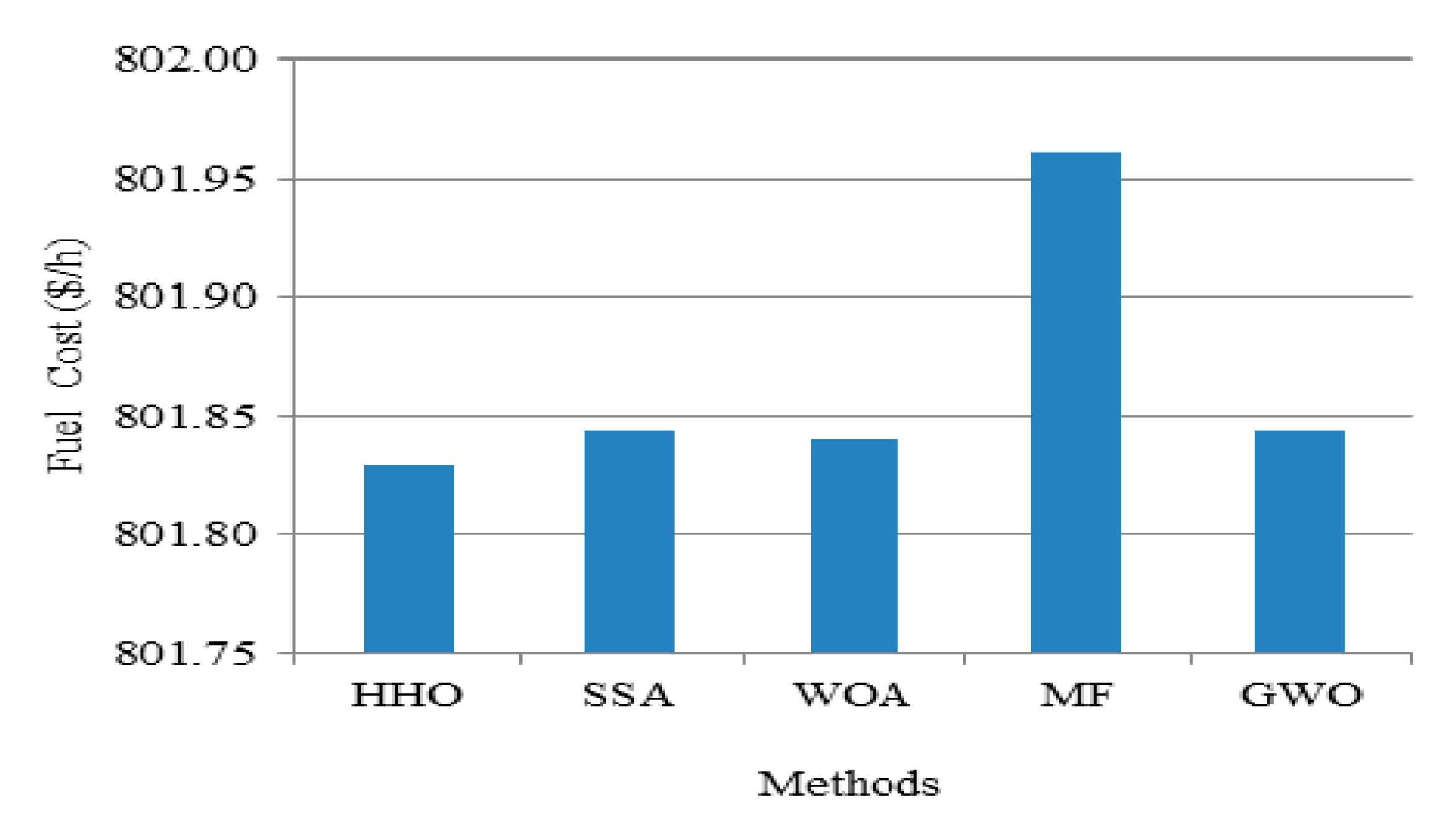
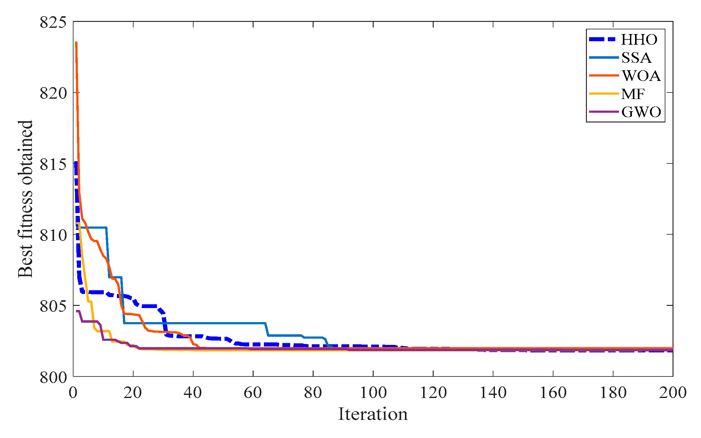
Case 1—Quadratic Total Fuel Cost Minimization

The quadratic fuel cost characteristics of a generator were chosen as the single-objective function to be minimized by the proposed HHO algorithm as defined in (1). The obtained optimal value of control variables by optimizing the total fuel cost (TFC) of the system is illustrated in

Table 3. Comparison of different methods for case 1.

Method	Items
	PG1 (MW)	PG2 (MW)	PG5 (MW)	PG8 (MW)	PG11 (MW)	PG13 (MW)	Cost ($/h)	Loss (MW)	Emission (ton/h)	Iteration (N)	Time (s)
HHO	176.97	48.88	21.42	22.02	12.29	11.21	801.829	9.387	1.263	132	58
SSA	176.78	48.83	21.47	21.65	12.09	12.00	801.844	9.376	1.274	135	62
WOA	176.80	48.94	21.50	21.65	12.13	12.00	801.840	9.393	1.270	197	64
MF	177.70	49.25	21.35	21.29	10.73	12.93	801.960	9.410	1.274	183	60
GWO	176.73	48.83	21.47	21.65	12.09	12.00	801.844	9.376	1.280	66	67

. To achieve this, the proposed method undergoes several stages of exploration and exploitation by dividing the search region in the space. Initially, the generators are initialized randomly by exploring the search regions and they give the various local solutions of TFC as $/h 842.131, $/h 835.204, $/h 828.532, $/h 814.891, and so on for different iterations. Then, the hawks undergo the soft and hard siege stages to find their global best by exploiting the solution in the search region to reach the global minima value of 801.829 as TFC. Hence, the obtained global solution is recorded as the best minimal value of TFC after 50 individual runs by the proposed method and compared with other nature-inspired methods. It is seen that the TFC is decreased to 801.829 $/h by the proffered method and its comparison with other intelligence algorithms is illustrated in Table 3. Thus, the HHO method optimized to give superior results for the selected single objective. In addition to the control parameters and TFC, the other computational parameters, such as real power loss, environmental emissions, iteration, and convergence time, are promising but stuck at a certain time and reported in Table 3. Additionally, the obtained fuel cost for various methods with its convergence characteristics is portrayed in Figure 4 and Figure 5.

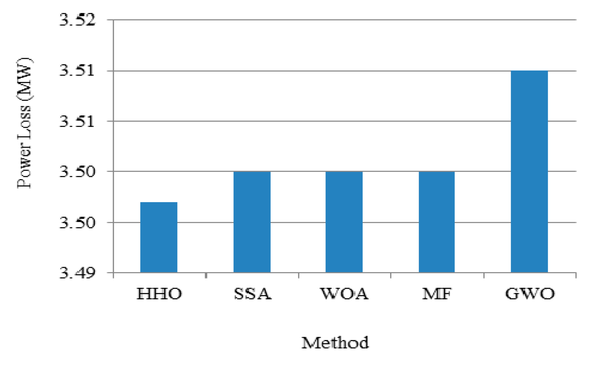
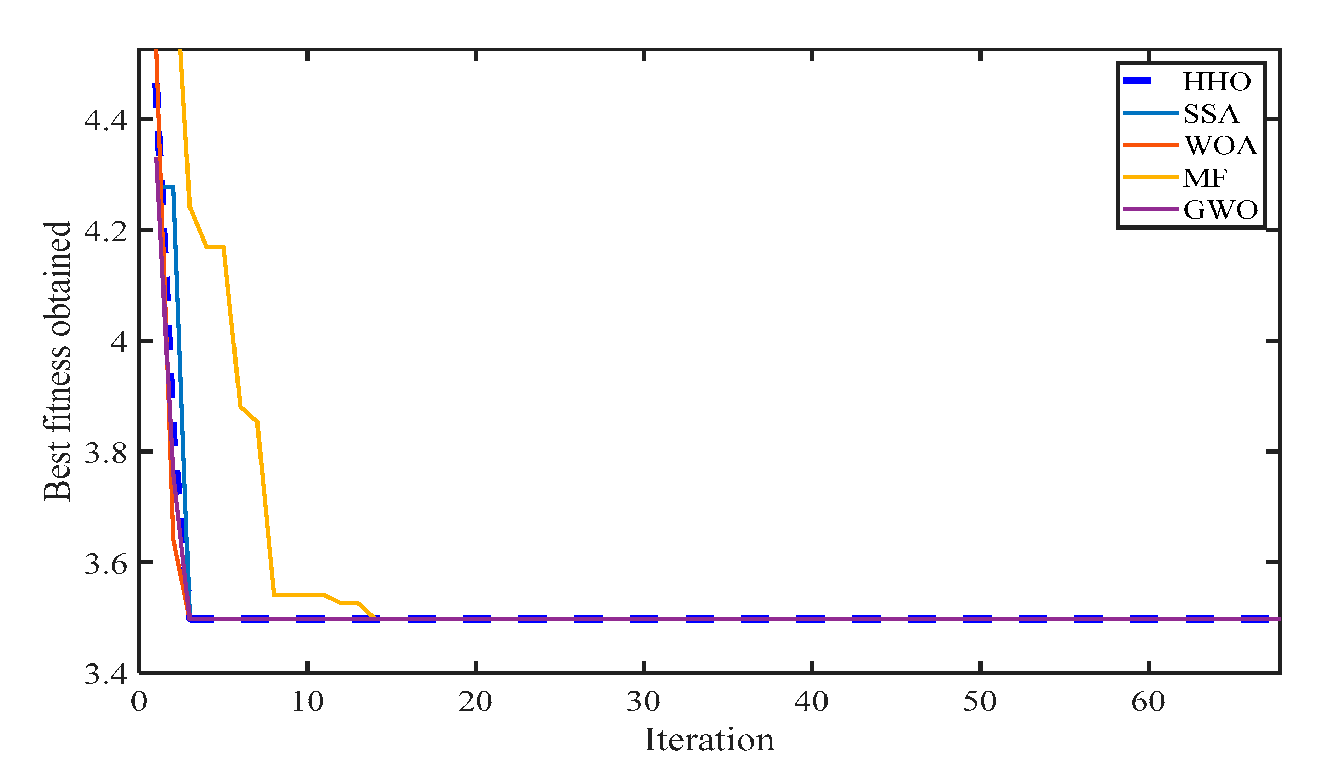
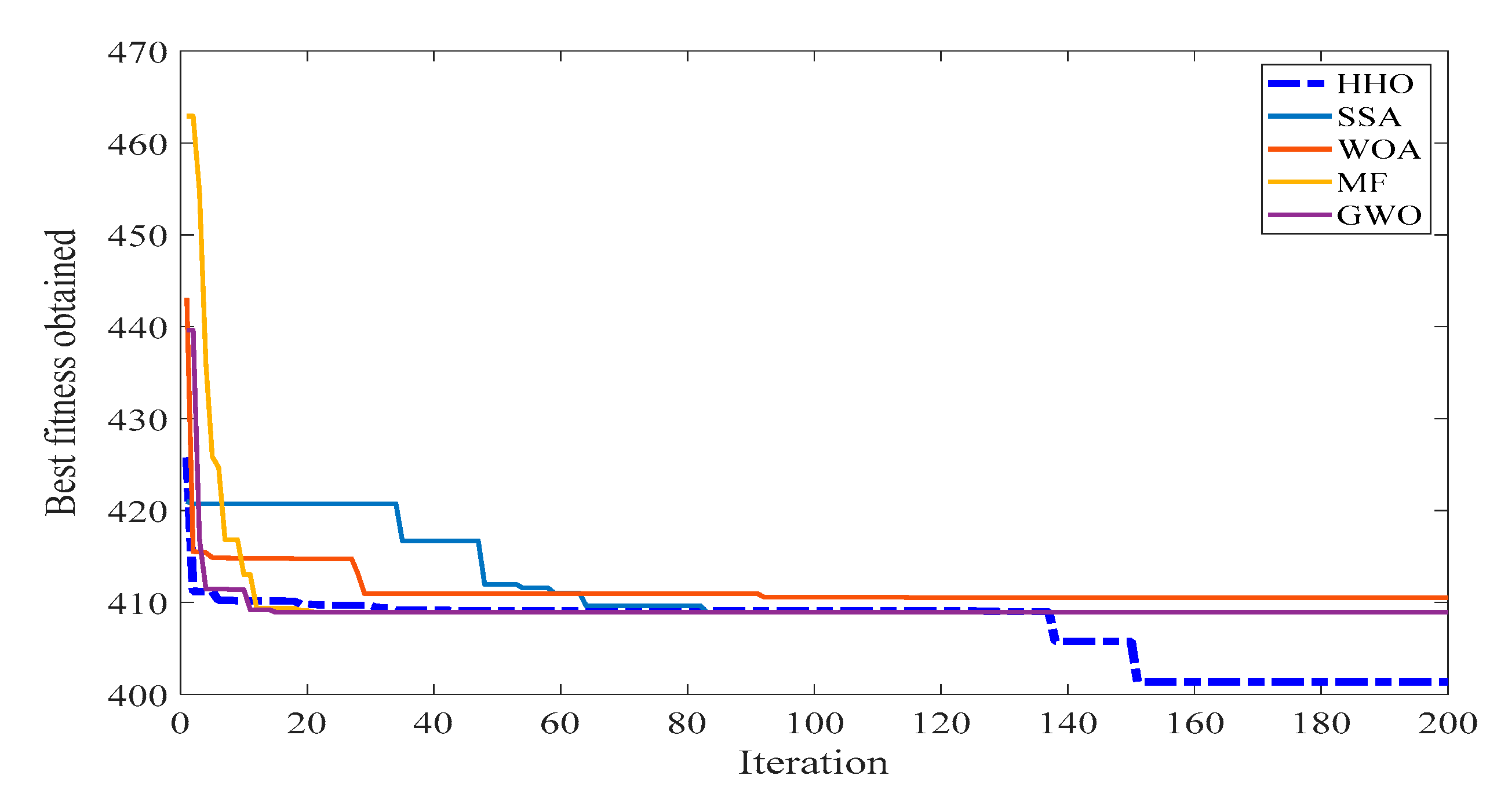
Case 2—Active Power Loss Minimization

To validate the effectiveness of the proposed method of OPF, the active power loss (APL) is regarded as a second single-objective function to be minimized and its formulation is represented in (2). The losses of the system can be minimized by optimally satisfying the load demand and the constraints of the system. The simulation results under this case are compared with other recent evolutionary meta-heuristic methods and are given in

Table 4. Different methods for case 2.

Method	Items
	PG1 (MW)	PG2 (MW)	PG5 (MW)	PG8 (MW)	PG11 (MW)	PG13 (MW)	Cost ($/h)	Loss (MW)	Emission (ton/h)	Iteration (N)	Time (s)
HHO	52.63	79.76	49.85	34.89	29.91	39.88	966.12	3.49	0.296	3	56
SSA	51.90	80.00	50.00	35.00	30.00	40.00	968.56	3.50	0.296	4	61
WOA	52.03	79.96	49.97	34.98	29.98	39.98	968.21	3.50	0.296	3	61
MF	51.90	80.00	50.00	35.00	30.00	40.00	968.56	3.50	0.296	21	62
GWO	52.10	80.00	50.00	34.80	30.00	40.00	968.29	3.51	0.297	3	65

. It can be seen that the APL in the IEEE 30-bus test system has declined to 3.49 MW and the performance of the proposed method is infinitesimally improved in comparison to other recent literatures such as the SSA, WOA, MF, and GWO presented above. In addition, the proffered method outperforms relative to the other methods to give a minimum TFC of 966.12 $/h. However, the performance is found similar to literature works for other computational parameters like emissions and number of iterations. In addition, the presented method takes a smaller amount of time for convergence. Figure 6 and Figure 7 portray the comparison of power loss minimization by various methods and its fitness curve, respectively. The results demonstrate that the proposed method attains the optimal solution with a minimum number of iterations and requires a shorter computation time because of its local and global search ability.

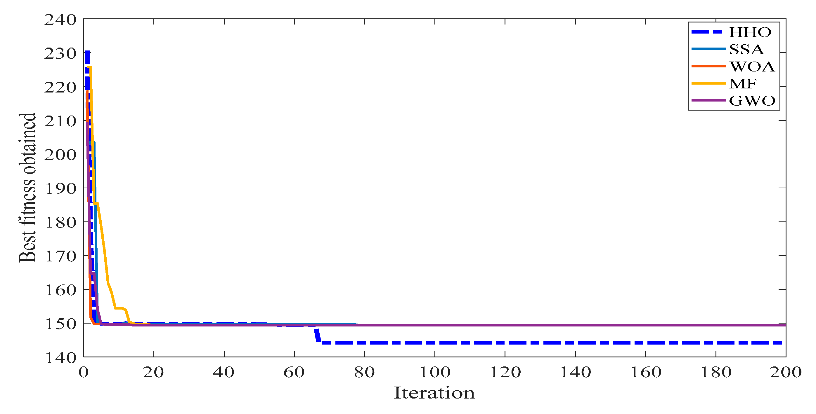
Case 3—Total Emission Cost Minimization

In this case, the total emission cost (TEC) is regarded as the third single-objective function to be minimized and its formulation is given in (3). The attained optimal values of control variables for minimization of TEC by the propounded method and the other techniques are illustrated in

Table 5. Different methods for case 3.

Method	Items
	PG1 (MW)	PG2 (MW)	PG5 (MW)	PG8 (MW)	PG11 (MW)	PG13 (MW)	Cost ($/h)	Loss (MW)	Emission (ton/h)	Iteration (N)	Time (s)
HHO	60.99	70.98	50.00	35.00	30.00	40.00	950.98	3.570	0.2850	32	56
SSA	61.02	70.95	50.00	35.00	30.00	40.00	950.93	3.600	0.2950	142	62
WOA	61.08	70.89	50.00	35.00	30.00	40.00	950.82	3.571	0.2950	39	62
MF	61.02	70.95	50.00	35.00	30.00	40.00	950.93	3.572	0.2950	29	61
GWO	60.93	71.12	50.00	34.93	30.00	40.00	951.13	3.571	0.2960	171	57

. The result based on the least emissions reveals that the proposed method outperforms compared to other presented literature work to give significant improvements and the TEC is reduced to 0.285 (ton/h).

Moreover, the computational parameters, such as losses and convergence time, are more enhanced than other evolutionary methods. The fuel cost is found to be similar to other techniques, but the proposed method takes a minimum number of iterations for the convergence of a solution. This inference is presented as Figure 8 and Figure 9 for better understanding, showing that the performance in reaching a global optimal solution by the hawks optimizer is better than other nature-inspired techniques.

Selection of Weightsfor Solving Multi-ObjectiveOPF Functions

In general, the multi-objective optimization can be solved with or without the preferences of specific objectives. However, the proposed work chooses the no preference weighted sum method. In this approach, the optimization problem aims to optimize all of the objectives with equal importance without giving prime importance to any of the objectives to be minimized. However, in order to study the assumed effects on weight based on the priority given to specific objectives, this work solves the two objectives (cost and loss) and three objective (cost, loss, and emission) using the proposed HHO method and its corresponding results are represented in

Table 6. Set of weights assumed for minimizing fuel cost and losses.

SL No	Weight		Cost ($/h)	Loss (MW)
	Cost	Loss
1	0.50	0.50	802.010	9.040
2	0.10	0.90	810.249	7.212
3	0.20	0.80	804.205	8.170
4	0.30	0.70	802.729	8.629
5	0.40	0.60	802.197	8.898
6	0.60	0.40	801.910	9.166
7	0.70	0.30	801.871	9.241
8	0.80	0.20	801.855	9.294
9	0.90	0.10	801.846	9.349

and

Table 7. Set of weights assumed for minimizing fuel cost, loss, and emission.

SL No	Weight			Cost ($/h)	Loss (MW)	Emission (ton/h)
	Cost	Loss	Emission
1	0.33	0.33	0.34	961.88	3.538	0.2982
2	0.20	0.20	0.60	938.679	3.798	0.299
3	0.40	0.40	0.20	880.708	4.688	0.353
4	0.60	0.20	0.20	860.872	5.074	0.399
5	0.20	0.60	0.20	906.061	4.231	0.321

. It is inferred that the solution obtained has no significant compromising results for different combinations of weight values assumed, and therefore an equal weight is considered for all of the objective functions. Additionally, in present days owing to the growth of renewable energy sources, the economy to improve the assets of generation, transmission, and distribution systems considering the environmental factors leads this research to choose the equal preference. On the flipside, solving three objective functions as multi-objective, the change in environmental conditions due to pollution is considered of prime importance with weight values of 0.34 than cost and losses for sustainable energy development.

Case 4—TFC and APL minimization

In this case, two prime contradictory objectives such as fuel cost and power loss were optimized simultaneously using the weighted sum method by the proposed HHO algorithm in Equation (7). The no preference weighted method has been chosen by assuming the sum of the weight values to be one (i.e., w1 = w2 = 0.5).

Table 8. Comparison of different methods for case 4.

Method	Items
	PG1 (MW)	PG2 (MW)	PG5 (MW)	PG8 (MW)	PG11 (MW)	PG13 (MW)	Cost ($/h)	Loss (MW)	Emission (ton/h)	Iteration (N)	Time (S)
HHO	172.56	48.86	22.01	24.12	12.88	12.00	802.01	9.040	1.2140	118	52
SSA	172.60	48.90	22.00	24.00	12.90	12.00	802.00	9.180	1.2150	148	78
WOA	174.25	50.05	22.31	20.94	12.97	12.10	801.97	9.218	1.2340	135	64
MF	172.61	48.93	22.00	24.02	12.90	12.00	802.00	9.051	1.2150	58	69
GWO	172.92	48.72	22.07	23.90	12.86	12.00	802.01	9.065	1.2193	197	59

shows the best optimal values of the control variables obtained by minimizing the TFC and APL. Additionally, the obtained results by the proffered method are compared with the literature work, such as SSA, WOA, MF, and GWO. It is seen that the HHO outperforms these to give superior results with a TFC of 802.01 (S/h) and an APL of 9.04 (MW). However, the value of TFC is minimum using WOA, but the APL is not reduced as compared to HHO. On the other hand, MF and GWO give similar results to optimize the selective fitness function but the emission cost increases relative to other techniques. Figure 10 demonstrates the convergence characteristics finding the optimal value of TFC and APL by HHO and various optimization methods. Overall, the performance of HHO for solving multi-objective OPF problem is decent compared to other presented techniques. Additionally, the obtained results of other computational parameters during optimization are promising.

Case 5—TFC and TEC Minimization

In this study, the fitness function to be optimized simultaneously in Equation (8) is fuel cost and environmental emissions; by adapting the control variables the objective function can be minimized by optimally satisfying the equality and inequality constraints. The obtained results for the IEEE30-bus system with the control variables and its variation for the proposed and other intelligence methods are depicted in

Table 9. Comparison of different methods for case 5.

Method	Items
	PG1 (MW)	PG2 (MW)	PG5 (MW)	PG8 (MW)	PG11 (MW)	PG13 (MW)	Cost ($/h)	Loss (MW)	Emission (ton/h)	Iteration (N)	Time (S)
HHO	72.91	79.80	38.12	34.88	30.69	31.29	903.22	4.290	0.3150	48	63
SSA	72.39	79.46	37.93	35.00	30.00	32.91	904.05	4.291	0.3211	145	72
WOA	72.62	74.17	38.36	34.98	29.98	37.52	905.38	4.220	0.3232	190	68
MF	71.73	77.70	39.73	35.00	30.00	33.44	907.41	4.191	0.3183	199	153
GWO	72.12	80.00	37.81	35.00	30.00	32.77	904.45	4.295	0.3207	35	68

. Table 9 represents the compromising solutions for the selected objective function such as TFC and TEC, and their values are recorded as 903.22 $/h and 0.315 ton/h, respectively. In addition, the TFC and TEC variations as a function of control variables for various iterations and their comparison with other intelligence methods are also illustrated in Figure 11. It is clearly inferred that the multi-objective function minimized by the proposed method and achieves promising results compared to other techniques.

Case 6—APL and TEC Minimization

In this phase, APL and TEC were considered as an objective function to be optimized in Equation (9). In general, the emission dispatching is directly concerned with the generating units. Thus, the fitness function is minimized by adjusting the control variables, and its variations for the proposed and other intelligence methods are depicted in

Table 10. Comparison of different methods for case 6.

Method.	Items
	PG1 (MW)	PG2 (MW)	PG5 (MW)	PG8 (MW)	PG11 (MW)	PG13 (MW)	Cost ($/h)	Loss (MW)	Emission (ton/h)	Iteration (N)	Time (S)
HHO	54.09	79.86	49.73	35.29	30.92	37.03	961.88	3.538	0.2982	63	48
SSA	54.67	80.00	50.00	35.00	30.00	37.27	961.76	3.543	0.2993	124	56
WOA	54.77	79.97	49.98	34.99	29.99	37.25	961.51	3.549	0.2954	24	63
MF	54.67	80.00	50.00	35.00	30.00	37.27	961.76	3.553	0.2953	32	74
GWO	55.30	79.84	50.00	35.00	29.61	37.21	960.49	3.558	0.2996	196	79

. Table 10 shows the compromising solution for both power loss and emission by fulfilling the constraints. It is found that the proposed HHO gives the best optimal solution for APL and TEC minimization of 3.538 MW and 0.298 ton/h, respectively. Figure 12 demonstrates the convergence property of the selected fitness function consisting of all compared methods. It is found from Table 10 that the intelligence methods like GWO give the best value for fuel cost (960.49 $/h), but the method gives pessimistic results for the actual objective function. Overall, it is observed that the HHO method gives optimistic results for the multi-objective function by controlling all the computational parameters of the OPF problem. The convergence performance is recorded at the lowest in terms of time and iteration by the proposed technique.

Case 7—TFC, APL, and TEC Minimization

In this case, three competing objective functions are optimized by the proposed HHO algorithm simultaneously using the weighted sum method with the weights of various functions like TFC, APL, and TEC as w₁ = 0.33, w₂ = 0.33, and w₃ = 0.34, respectively. Equation (10) represents the objective function to be minimized by optimally dispatching the generating units and satisfying the power flow constraints.

Table 11. Comparison of different methods for case 7.

Method.	Items
	PG1 (MW)	PG2 (MW)	PG5 (MW)	PG8 (MW)	PG11 (MW)	PG13 (MW)	Cost ($/h)	Loss (MW)	Emission (ton/h)	Iteration (N)	Time (S)
HHO	71.25	78.67	38.40	35.00	32.10	32.19	906.52	4.21	0.297	149	55
SSA	71.74	79.56	38.33	35.00	30.00	33.04	905.73	4.26	0.320	150	73
WOA	70.21	78.56	37.77	33.19	30.00	37.92	910.57	4.26	0.320	195	63
MF	71.74	79.56	38.33	35.00	30.00	33.04	905.73	4.26	0.320	165	64
GWO	71.66	79.29	38.50	34.98	30.00	33.23	906.10	4.25	0.320	199	63

shows the result obtained by the proposed and other intelligence methods. The best optimal values are recorded for APL of 4.21 MW and TEC of 0.29 ton/h by the HHO method and its performance is reasonable for a TFC of 906.52 $/h. On the flipside, the TFC is well optimized by the SSA and MF methods, but it seems to give pessimistic results for other objectives such as APL and TEC. Finally, it is clear that the obtained results of TFC, APL, and TEC cannot be further improved without degrading the performance of other parameters by all the intelligence methods presented. However, from inspection of the convergence curve portrayed in Figure 13, it can be inferred that the proposed HHO algorithm outperforms the other intelligence techniques to give a minimum value of fitness function.

Case 7a—Minimization of TFC, APL, and TEC with presence of 5 MW DG

This case is similar to case 7 with the presence of DG for reducing the losses and emission costs of the system. The optimal location of DG is done using a real power sensitivity analysis based on the procedure detailed in [53].

Table 12. Ranking of 5 MW DG placement based on the real power sensitivity index.

S. No	Loss Sensitivities		Rank	Loss Reduction (%)
	∂Ploss/∂P	Bus		With 5MW DG
1	−0.1359	30	1	9.8355
2	−0.1106	26	2	7.8998
3	−0.1093	29	3	7.19537
4	−0.0906	24	4	7.16288
5	−0.0888	19	5	7.0072
6	−0.0857	18	6	6.7302
7	−0.0853	25	7	6.6088
8	−0.0845	23	8	6.5592
9	−0.0824	20	9	6.5165
10	−0.0733	21	10	5.9539
11	−0.0729	22	11	5.9078
12	−0.0722	15	12	5.8154
13	−0.0714	27	13	5.6906
14	−0.069	7	14	5.6718
15	−0.0657	14	15	5.3024
16	−0.0645	17	16	5.21015
17	−0.0644	28	17	4.9946
18	−0.0596	10	18	4.8955
19	−0.0593	16	19	4.8647
20	−0.0588	9	20	4.8561
21	−0.0584	6	21	4.6817
22	−0.0498	4	22	4.1363
23	−0.0462	12	23	3.7601
24	−0.0391	3	24	3.2249

depicts the ranking for placement of DG based on estimated sensitivity index. It is observed that bus 30 is the critical candidate bus with a maximum magnitude of index value of 0.1359 compared to all other load buses in the IEEE30-bus system. Thus, the placement of 5 MW DG in the 30-bus system results in the generation dispatch of PG1, PG2, PG5, PG8, PG11, and PG13 as 71.66 MW, 79.53 MW, 38.54 MW, 35 MW, 30 MW, and 32.88 MW, respectively. The result shows that the TFC, APL, and TEC of the system have been reduced from $/h 906.52 to $/h 905.19, 4.21 MW to 4.02 MW, and 0.297 ton/h to 0.219 ton/h, respectively, compared to the normal case as depicted in

Table 13. Comparison of TFC, APL, and TEC performance with and without DG using HHO.

HHO	Cost ($/h)	Loss (MW)	Emission (ton/h)	Iteration (N)	Time (S)
Without DG	906.52	4.21	0.297	149	55
With DG	905.19	4.02	0.219	142	52

. It is inferred that the change is not very significant for all the three parameters considered. However, the type of DG considered is of a smaller size and the optimal sizing of the DG needs to be done for remarkable changes in the parameters. However, the scope of this study is limited to analyze the effect of DG placement on system losses and emissions. The result also reveals that the losses and emissions of the system are reduced to 9.8355% and 26.2%, respectively, which enhances the sustainable power generation.

5. Comparative Analysis

In this section, the performance of HHO-based OPF to minimize the TFC is only considered for comparison with the literature work because of its prime importance in the electric sector compared to any other OPF objectives.

Table 14. Comparative analysis on performance of HHO with recent literature works.

Methods	PG1	PG2	PG5	PG8	PG11	PG13	Fuel Cost ($/h)	% Improvement
HHO	176.97	48.88	21.42	22.02	12.29	11.21	801.829	0.023
TLBO [26]	177.3986	48.0701	21.7722	21.89616	12.08228	11.61326	801.9908	0.0028
MTLBO [26]	177.2561	48.0762	21.1925	22.1182	12.1124	11.821	801.8925	0.0151
TS [29]	176.04	48.76	21.56	22.05	12.44	12	802.29	−0.0344
EP [55]	173.848	49.998	21.386	22.63	12.928	12	802.62	−0.0756
IEP [56]	176.2358	49.0093	21.5023	21.8115	12.3387	12.0129	802.465	−0.0562
DE [57]	176.009	49	21.334	22.262	12.46	12	802.394	−0.0474
MDE [57]	175.974	49	21.51	22.24	12.251	12	802.376	−0.0452
SS [58]	193	48	19.5506	11.6204	10	12	804.1072	−0.261
EGA [59]	176.2	49	21.44	21.95	12.42	12.02	802.06	−0.0058
ACO [60]	181.945	47.001	21.4596	21.446	13.207	12.0134	802.578	−0.0703
FGA [61]	175.137	50.353	21.451	21.176	12.667	12.11	802.0003	0.00166
PSO [62]	175.6915	48.639	21.4494	22.72	12.2302	12	802.0136	Benchmark
MHBMO [63]	177.0431	49.209	21.5135	22.648	10.4146	12	801.985	0.0036
HBMO [63]	176.4646	46.274	21.4596	21.446	13.207	12.0134	802.211	−0.0246

illustrates the various optimization methods for minimizing the fuel cost whilst optimizing the control parameters such as real power generation of generators. It is seen from the results that the Stochastic Search algorithm (SS) shows the worst optimized TFC of 804.1072 $/h by uneconomical dispatches of the generators PG1 (193 MW) and PG8 (11.62 MW). On the flipside, Tabu search (TS), Evolutionary Programming(EP), Differential Evolution(DE), Modified Differential Evolution (MDE), the Enhanced Genetic Algorithm (EGA), and Ant Colony Optimization(ACO) exhibit TFC in the range of 802 $/h to 802.7 $/h. Additionally, the Modified Honey Bee Mating Optimization (MHBMO), Teaching Learning-Based Optimization (TLBO), and Modified TLBO showed that the TFC is optimized in the range between 801.8925 $/h and 801.985 $/h. However, the proposed HHO technique outperforms these to give the TFC of 801.829 $/h, indicating the best optimal solution among the various methods presented. Additionally, the % improvement of the proposed HHO method has been evaluated by choosing the PSO technique as a benchmark method. The result claims that the proffered method can significantly outperform by 0.023% more than the PSO compared to other optimization techniques. Additionally, the performance of TS, EP, IEP, DE, MDE, SS, EGA, ACO, and HBMO is not superior to that of the PSO method, which shows the solutions obtained from these optimization methods are not feasible. Among all the techniques the SS method underperforms by an amount of 0.26% compared to the PSO method. However, the proposed HHO method demonstrates its better performance through the exploration and exploitation characteristics of Hawks to tune the parameters of the generator output power. This claim makes the HHO better to optimize the generator parameters for a different combination of objective functions considered.

6. Conclusions

A novel nature-inspired Harris Hawks Optimization (HHO) method has been proposed to solve the single and multi-objective OPF problem of power systems. In this work, various conflicting single and multi-objectives are framed using total fuel cost, active power loss, and environmental emission cost with the concern of reducing the environmental emissions from thermal generating units. In this work, equal importance is given to all three objectives, because the electric sector is aiming to compensate all the three factors as its prime objectives. Hence, a no-preference weighted sum approach has been used to solve the multi-objective OPF problem. The effectiveness of the proffered method was tested on an IEEE 30-bus system by optimally setting the control variables. The results obtained for different cases were compared with the other well-known nature-inspired intelligence techniques like SSA, WOA, MF, and GWO. It is seen that the HHO performance improved predominantly from 0.01% to 0.37% for various disparate cases of selective objective function compared to other methods. Additionally, the study on the placement of 5 MW DG based on a sensitivity analysis revealed that the system losses and emissions are reduced by an amount of 9.8355% and 26.2%, respectively, compared to conventional thermal power generators. The analysis on the sizing of DG and a contingency analysis will be the future scope of the work.

References

1. Dommel, H.W.; Tinney, W.F. Optimal Power Flow Solutions. Stud. Syst. Decis. Control 1968, PAS−87, 1866–1876. [Google Scholar] [CrossRef]
2. Abaci, K.; Yamacli, V. Differential search algorithm for solving multi-objective optimal power flow problem. Int. J. Electr. Power Energy Syst. 2016, 79, 1–10. [Google Scholar] [CrossRef]
3. Zhu, J.Z. Improved interior point method for OPF problems—Power Systems. IEEE Trans. Power Syst. 1999, 14, 1114–1120. [Google Scholar]
4. Veerapandiyan, V.; Mary, D. Transmission System Reconfiguration to Reduce Losses and Cost Ensuring Voltage Security. J. Power Energy Eng. 2016, 4, 4–12. [Google Scholar]
5. Warid, W.; Hizam, H.; Mariun, N.; Izzri, N.; Wahab, A.; Wahab, N.I.A. A novel quasi-oppositional modified Jaya algorithm for multi-objective optimal power flow solution. Appl. Soft Comput. J. 2018, 65, 360–373. [Google Scholar] [CrossRef]
6. Salgado, R.; Brameller, A.; Aitchison, P. Optimal power flow solutions using the gradient projection method. Part 1. Theoretical basis. IEE Proc. C Gener. Transm. Distrib. 1990, 137, 424–428. [Google Scholar] [CrossRef]
7. Tinney, W.F.; Member, S.; Hart, C.E. Power Flow Solution by Newton’s Method. Proc. IEEE 1967, 86, 1459–1467. [Google Scholar] [CrossRef]
8. Momoh, J.A. A Review of Selected Optimal Power Ftow Literature to 1993 Part I: Non Linear and Quadratic Programming Approaches. IEEE Trans. Power Syst. 1999, 14, 96–104. [Google Scholar] [CrossRef]
9. Olofsson, M.; Andersson, G.; Söder, L. Linear programming based optimal power flow using second order sensitivities. IEEE Trans. Power Syst. 1995, 10, 1691–1697. [Google Scholar] [CrossRef]
10. Torres, G.L.; Quintana, V.H.; Engineering, E. AN interior-point method for nonlinear optimal power flow using voltage rectangular coordinates. IEEE Trans. Power Syst. 1998, 13, 1211–1218. [Google Scholar] [CrossRef]
11. Fortenbacher, P.; Demiray, T. Linear/quadratic programming-based optimal power flow using linear power flow and absolute loss approximations. Int. J. Electr. Power Energy Syst. 2019, 107, 680–689. [Google Scholar] [CrossRef] [Green Version]
12. Ferreira, R.S.; Borges, C.L.T.; Pereira, M.V.F. A flexible mixed-integer linear programming approach to the AC optimal power flow in distribution systems. IEEE Trans. Power Syst. 2014, 29, 2447–2459. [Google Scholar] [CrossRef]
13. Veerapandiyan, V.; Mary, D. A Comparative Method of Optimal Power Flow for Ieee−30 Bus System. 2015, 10, 359–364. Int. J. Appl. Eng. Res. 2015; 10, 359–364. [Google Scholar]
14. MOsman, S.; Abo-Sinna, M.A.; Mousa, A.A. A solution to the optimal power flow using genetic algorithm. Appl. Math. Comput. 2004, 155, 391–405. [Google Scholar]
15. Yuan, X.; Zhang, B.; Wang, P.; Liang, J.; Yuan, Y.; Huang, Y.; Lei, X. Multi-objective optimal power flow based on improved strength Pareto evolutionary algorithm. Energy 2017, 122, 70–82. [Google Scholar] [CrossRef]
16. Shukla, A.; Tiwari, R.; Kala, R. Genetic programming. Stud. Comput. Intell. 2010, 307, 209–234. [Google Scholar]
17. Bhattacharya, A.; Chattopadhyay, P.K. Solution of optimal reactive power flow using biogeography-based optimization. World Acad. Sci. Eng. Technol. 2009, 39, 852–860. [Google Scholar]
18. Sakthivel, S.; Pandiyan, S.A.; Marikani, S.; Selvi, S.K. Application of Big Bang Big Crunch Algorithm for Optimal Power Flow Problems. Int. J. Eng. Sci. 2013, 2, 41–47. [Google Scholar]
19. Duman, S.; Güvenç, U.; Sönmez, Y.; Yörükeren, N. Optimal power flow using gravitational search algorithm. Energy Convers. Manag. 2012, 59, 86–95. [Google Scholar] [CrossRef]
20. Gabash, A.; Li, P. Active-reactive optimal power flow in distribution networks with embedded generation and battery storage. IEEE Trans. Power Syst. 2012, 27, 2026–2035. [Google Scholar] [CrossRef]
21. Moghaddas, S.M.J.; Samani, H.M.V. Application of Central Force Optimization Method to Design Transient Protection Devices for Water Transmission Pipelines. Mod. Appl. Sci. 2016, 11, 76. [Google Scholar] [CrossRef] [Green Version]
22. Hariharan, T.; Sundaram, K.M. Multiobjective optimal power flow using Particle Swarm Optimization. Int. J. Control Theory Appl. 2016, 80, 128–139. [Google Scholar]
23. Mohamed, A.A.A.; El-Gaafary, A.A.M.; Mohamed, Y.S.; Hemeida, A.M. Multi-objective Modified Grey Wolf Optimizer for Optimal Power Flow. In Proceedings of the 2016 Eighteenth International Middle East Power Systems Conference (MEPCON), Cairo, Egypt, 27–29 December 2016; pp. 982–990. [Google Scholar]
24. Reddy, S.S.; Rathnam, C.S. Electrical Power and Energy Systems Optimal Power Flow using Glowworm Swarm Optimization. Int. J. Electr. Power Energy Syst. 2016, 80, 128–139. [Google Scholar] [CrossRef]
25. Sayed, G.I.; Khoriba, G.; Haggag, M.H. A novel chaotic salp swarm algorithm for global optimization and feature selection. Appl. Intell. 2018, 48, 3462–3481. [Google Scholar] [CrossRef]
26. Shabanpour-Haghighi, A.; Seifi, A.R.; Niknam, T. A modified teaching-learning based optimization for multi-objective optimal power flow problem. Energy Convers. Manag. 2014, 77, 597–607. [Google Scholar] [CrossRef]
27. Li, Y.Z.; Li, M.S.; Ji, Z.; Wu, Q.H. Optimal power flow using group search optimizer with intraspecific competition and lévy walk. In Proceedings of the2013 IEEE Symposium on Swarm Intelligence (SIS 2013), Singapore, 16–19 April 2013; pp. 256–262. [Google Scholar]
28. Sivasubramani, S.; Swarup, K.S. Multi-objective harmony search algorithm for optimal power flow problem. Int. J. Electr. Power Energy Syst. 2011, 33, 745–752. [Google Scholar] [CrossRef]
29. Abido, M.A. Optimal power flow using tabu search algorithm. Electr. Power Components Syst. 2002, 30, 469–483. [Google Scholar] [CrossRef] [Green Version]
30. Gogna, A.; Tayal, A. Metaheuristics: Review and application. J. Exp. Theor. Artif. Intell. 2013, 25, 503–526. [Google Scholar] [CrossRef]
31. Adaryani, M.R.; Karami, A. Artificial bee colony algorithm for solving multi-objective optimal power flow problem. Int. J. Electr. Power Energy Syst. 2013, 53, 219–230. [Google Scholar] [CrossRef]
32. Yang, X. Multiobjective Firefly Algorithm for Continuous Optimization; Springer: Berlin, Germany, 2016. [Google Scholar]
33. Mukherjee, A.; Mukherjee, V. Solution of optimal power flow using chaotic krill herd algorithm. Chaos Solitons Fractals 2015, 78, 10–21. [Google Scholar] [CrossRef]
34. Ayan, K.; Kiliç, U. Optimal power flow of two-terminal HVDC systems using backtracking search algorithm. Int. J. Electr. Power Energy Syst. 2016, 78, 326–335. [Google Scholar] [CrossRef]
35. Reddy, S.S.; Bijwe, P. Multi-Objective Optimal Power Flow Using Efficient Evolutionary Algorithm. Int. J. Emerg. Electr. Power Syst. 2017, 18. [Google Scholar] [CrossRef]
36. Reddy, S.S.; Bijwe, P.R.; Abhyankar, A.R. Faster evolutionary algorithm based optimal power flow using incremental variables. Int. J. Electr. Power Energy Syst. 2014, 54, 198–210. [Google Scholar] [CrossRef]
37. Daryani, N.; Hagh, M.T.; Teimourzadeh, S. Adaptive group search optimization algorithm for multi-objective optimal power flow problem. Appl. Soft Comput. J. 2016, 38, 1012–1024. [Google Scholar] [CrossRef]
38. el Ela, A.A.A.; Abido, M.A.; Spea, S.R. Optimal power flow using differential evolution algorithm. Electr. Power Syst. Res. 2010, 80, 878–885. [Google Scholar] [CrossRef]
39. Chen, H.; Bo, M.L.; Zhu, Y. Multi-hive bee foraging algorithm for multi-objective optimal power flow considering the cost, loss, and emission. Int. J. Electr. Power Energy Syst. 2014, 60, 203–220. [Google Scholar] [CrossRef]
40. Pirnia, M.; Canizares, C.A.; Bhattacharya, K.; Vaccaro, A. A novel affine arithmetic method to solve optimal power flow problems with uncertainties. IEEE Trans. Power Syst. 2014, 29, 2775–2783. [Google Scholar] [CrossRef]
41. Vaccaro, A.; Cañizares, C.A. A knowledge-based framework for power flow and optimal power flow analyses. IEEE Trans. Smart Grid 2018, 9, 230–239. [Google Scholar] [CrossRef]
42. Karbalaei, F.; Shahbazi, H.; Mahdavi, M. A new method for solving preventive security-constrained optimal power flow based on linear network compression. Int. J. Electr. Power Energy Syst. 2018, 96, 23–29. [Google Scholar] [CrossRef]
43. Can, U.; Alatas, B. Physics Based Metaheuristic Algorithms for Global Optimization. Am. J. Inf. Sci. Comput. Eng. 2015, 1, 94–106. [Google Scholar]
44. Niknam, T.; Narimani, M.r.; Jabbari, M.; Malekpour, A.R. A modified shuffle frog leaping algorithm for multi-objective optimal power flow. Energy 2011, 36, 6420–6432. [Google Scholar] [CrossRef]
45. El-Sattar, S.A.; Kamel, S.; el Sehiemy, R.A.; Jurado, F.; Yu, J. Single- and multi-objective optimal power flow frameworks using Jaya optimization technique. Neural Comput. Appl. 2019. [Google Scholar] [CrossRef]
46. Ma, R.; Li, X.; Luo, Y.; Wu, X.; Jiang, F. Multi-objective dynamic optimal power flow of wind integrated power systems considering demand response. CSEE J. Power Energy Syst. 2019, 5, 466–473. [Google Scholar] [CrossRef]
47. Khunkitti, S.; Siritaratiwat, A.; Premrudeepreechacharn, S.; Chatthaworn, R.; Watson, N.R. A hybrid DA-PSO optimization algorithm for multiobjective optimal power flow problems. Energies 2018, 11, 2270. [Google Scholar] [CrossRef] [Green Version]
48. Davoodi, E.; Babaei, E.; Mohammadi-ivatloo, B. An efficient covexified SDP model for multi-objective optimal power flow. Int. J. Electr. Power Energy Syst. 2018, 102, 254–264. [Google Scholar] [CrossRef]
49. Heidari, A.A.; Mirjalili, S.; Faris, H.; Aljarah, I.; Mafarja, M.; Chen, H. Harris hawks optimization: Algorithm and applications. Futur. Gener. Comput. Syst. 2019, 97, 849–872. [Google Scholar] [CrossRef]
50. Deb, K. Multi-Objective Optimization Using Evolutionary Algorithms, 1st ed.; John Wiley & Sons: Hoboken, NJ, USA, 2001; Volume 16. [Google Scholar]
51. Mazza, A.; Chicco, G.; Russo, A. Optimal multi-objective distribution system reconfiguration with multi criteria decision making-based solution ranking and enhanced genetic operators. Int. J. Electr. Power Energy Syst. 2014, 54, 255–267. [Google Scholar] [CrossRef]
52. Marler, R.T.; Arora, J.S. The weighted sum method for multi-objective optimization: New insights. Struct. Multidiscip. Optim. 2010, 41, 853–862. [Google Scholar] [CrossRef]
53. Warid, W.; Hizam, H.; Mariun, N.; Abdul-Wahab, N.I. A sensitivity based methodology for optimal placement of distributed generation in meshed power systems. Int. J. Simul. Syst. Sci. Technol. 2017, 17, 44.1–44.8. [Google Scholar]
54. IEEE 30-Bus Test System Data. Available online: www.ee.washington.edu/research/pstca/pf30/pg_tca30bus.httm (accessed on 28 January 2020).
55. Yuryevich, J.; Wong, K.P. Evolutionary programming based optimal power flow algorithm. IEEE Power Eng. Rev. 1999, 19, 54. [Google Scholar]
56. Costa, A.L.; Costa, A.S. Energy and ancillary service dispatch through dynamic optimal power flow. Electr. Power Syst. Res. 2007, 77, 1047–1055. [Google Scholar] [CrossRef]
57. Sayah, S.; Zehar, K. Modified differential evolution algorithm for optimal power flow with non-smooth cost functions. Energy Convers. Manag. 2008, 49, 3036–3042. [Google Scholar] [CrossRef]
58. Sliman, L.; Bouktir, T. |Economic Power Dispatch of Power System with Pollution Control using Multiobjective Ant Colony Optimization. Int. J. Comput. Intell. Res. 2007, 3, 2. [Google Scholar] [CrossRef]
59. Bakirtzis, A.G.; Biskas, P.N.; Zoumas, C.E.; Petridis, V. Optimal power flow by enhanced genetic algorithm. IEEE Trans. Power Syst. 2002, 17, 229–236. [Google Scholar] [CrossRef]
60. Bouktir, T.; Slimani, L.; Mahdad, B. Optimal power dispatch for large scale power system using stochastic search algorithms. Int. J. Power Energy Syst. 2008, 28, 118–126. [Google Scholar] [CrossRef]
61. Saini, A.; Chaturvedi, D.K.; Saxena, A.K. Optimal power flow solution: A GA-fuzzy system approach. Int. J. Emerg. Electr. Power Syst. 2006, 5, 1–23. [Google Scholar] [CrossRef]
62. Attous, D.B.; Labb, Y. Particle swarm optimisation based optimal power flow for units with non-smooth fuel cost functions. Model. Meas. Control A 2010, 83, 24–37. [Google Scholar]
63. Niknam, T.; Narimani, M.R.; Aghaei, J.; Tabatabaei, S.; Nayeripour, M. Modified Honey Bee Mating Optimisation to solve dynamic optimal power flow considering generator constraints. IET Gener. Transm. Distrib. 2011, 5, 989–1002. [Google Scholar] [CrossRef]
Figure 1. Classification of methods.
Sustainability 12 05248 g001
Figure 2. Patterns of Harris Hawks.
Sustainability 12 05248 g002
Figure 3. Single and multi-objective optimal power flow.
Sustainability 12 05248 g003
Figure 4. TFC for various intelligence methods.
Sustainability 12 05248 g004
Figure 5. Curve for case 1.
Sustainability 12 05248 g005
Figure 6. APL for Intelligence methods.
Sustainability 12 05248 g006
Figure 7. Curve for case 2.
Sustainability 12 05248 g007
Figure 8. TEC for various intelligencemethods.
Sustainability 12 05248 g008
Figure 9. Curve for case 3.
Sustainability 12 05248 g009
Figure 10. Convergence Curve for case 4.
Sustainability 12 05248 g010
Figure 11. Convergence curvefor case 5.
Sustainability 12 05248 g011
Figure 12. Curve for case 6.
Sustainability 12 05248 g012
Figure 13. Curve for case 7.
Sustainability 12 05248 g013