The Impact of Urban Transportation Infrastructure on Air Quality

Abstract

While previous study has confirmed significant correlation between infrastructure construction and air quality, little is known about the nature of the relationship. In this paper, we intend to fill this gap by using the Panel Smooth Transition Regression (PSTR) model to discuss the nonlinear relationship between transportation infrastructure construction and air quality. The panel data includes 280 cities in China for the period 2000-2017. We find that the transportation infrastructure investment is positively correlated to the air quality when the GDP per capita is below RMB 7151 or the number of motor vehicle population per capita is below 37 (vehicles per 10,000 persons) where the model is in the lower regime, and that the transportation infrastructure investment is negatively correlated to the air quality when the GDP per capita is greater than RMB 7151 or the number of motor vehicle population per capita is larger than 37 (vehicles per 10,000 persons) where the model is in the upper regime. The empirical results of the three sub-samples, including eastern, western and central regions, are similar to that of the national level. Furthermore, increasing transportation infrastructure investment is conducive to improving air quality. Urban bus services, green area, population density, wind speed and rainfall are also conducive to reducing air pollution, but the role of environmental regulation is not significant. After adding the instrumental variable (urban built-up area), the conclusions are further supported. Finally, relevant policy recommendations for reducing air pollution are proposed based on the empirical results.

1. Introduction

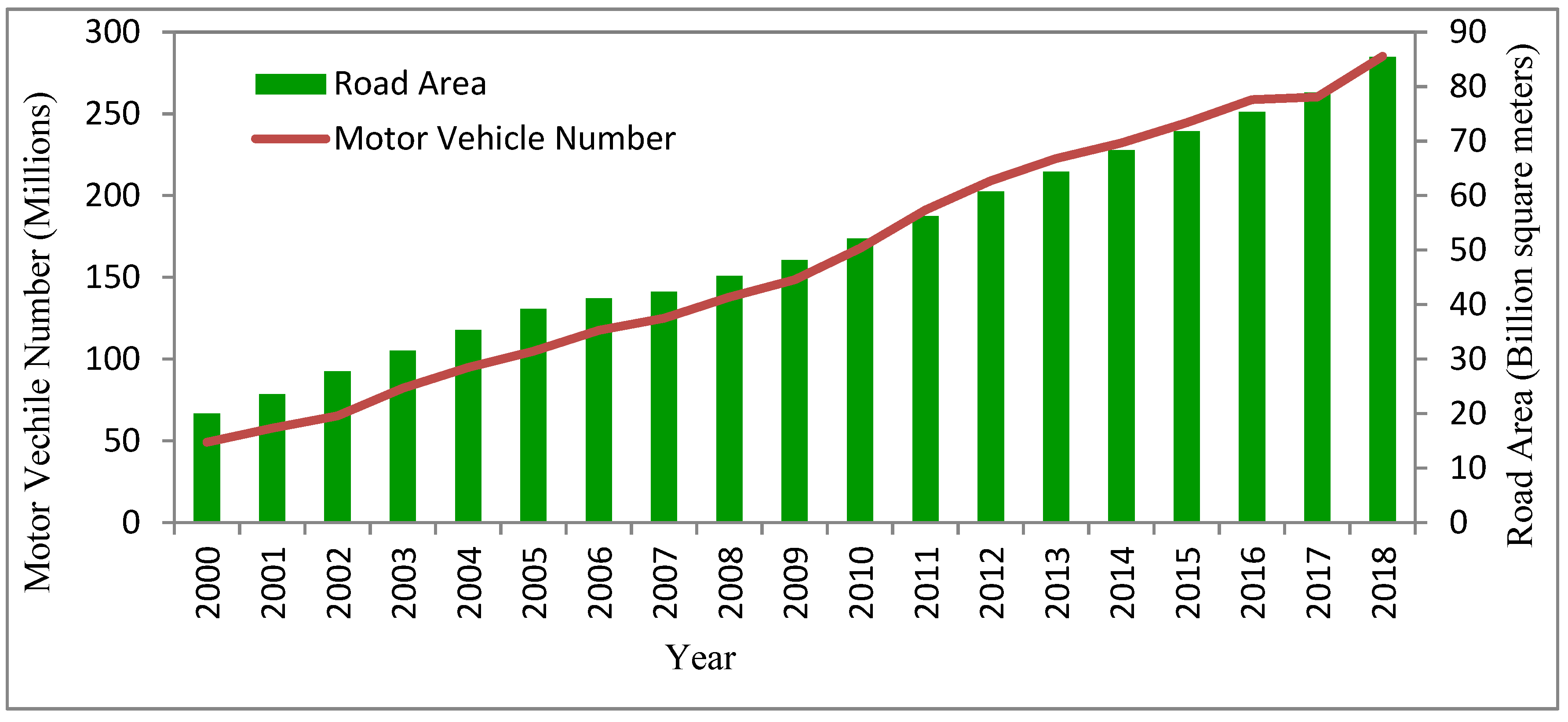
Data from the World Bank show that the proportion of the world’s urban population rose from 46.69% in 2000 to 55.27% in 2018, an increase of 8.58% In the rapid development of urbanization, the rapid population concentration and the population increase have resulted in an increase in the demand for commuting travel and logistics transportation. Therefore, pollution caused by motor vehicle exhaust has become one of the main sources of urban air pollution [1]. In 2019, the 2018 World Air Quality Report published on Air Visual showed that 89% of cities in China have exceeded the global air quality standard. The relatively backward construction of public transport infrastructure will lead to traffic congestion and other urban maladies, further aggravating the air pollution caused by traffic circulation. The Wind database indicates that the average annual growth rate of motor vehicle numbers was 10.96% from 2000 to 2017, while the road area growth rate during the same period was only 8.04% in China, as shown in Figure 1. The growth rate of vehicle consumption is higher than the growth rate of road construction. The vehicle growth causes slow speed and congestion, which will result in the fuel combusting insufficiently, and the pollutants from the exhaust gas are 2–3 times higher than that during normal driving [2]. Traffic congestion exacerbates urban air pollution, therefore, improving the traffic environment is an effective way to improve urban air quality [3].

The study found that transportation infrastructure has either a positive or negative effect on air quality. Some scholars suggest that increasing transportation infrastructure investment is conducive to improving air quality. The government takes effective measures to increase road investments, which can increase unblocked road traffic, avoid congestion and improve air quality [4,5,6]. Some scholars believe that the increase in subways [7], bus rapid transit [8], intercity railways [9], light rail [10] and other public transport means we can replace the high pollution from private cars, reducing PM_2.5, SO₂, NO₂, CO and NO emissions. However, Vickrey found increasing urban transportation investments make more convenient travel [11]. The convenience stimulates consumers to buy more cars, releasing more SO₂ emission [12,13]. Other scholars believe that the increase in transportation infrastructure investment makes industrial transportation more convenient and frequent, thereby bringing more negative effects such as industrial emissions and pollution [14,15,16,17]. Although the increase in transportation infrastructure is designed to achieve smooth traffic and reduce exhaust pollution, it requires large consumption of infrastructure investment capital [18]. The large capital consumption may impair environmental protection projects and environmental supervision, thereby resulting in deterioration of air quality in the long run. Ahmad believes that the increase in urban transportation investment is not a feasible plan to reduce emissions, because upgrading existing road facilities will take a lot of time and will lead to more traffic congestion [19]. The conclusion on the relationship between transportation infrastructure and air pollution is still controversial.

Most of the current studies adopt a linear perspective and ignore the nonlinear influence of transportation infrastructure construction on air quality. According to Duggal, ignoring nonlinearity will cause biased and inconsistent estimates of the results [20]. There are three reasons for the nonlinear relationship between transportation infrastructure construction and air pollution. First, it brings about changes in people’s common values of environment. Max Weber, in 1922, stated, “The use of public transport arises more from a system of values with which the person identifies than from the quality of the transport offered.” Carlos suggested that a higher index of postmodern values implies greater environmental awareness, which would lead to a greater use of sustainable transport [21]. People’s environmental values are different in different periods, and people’s influence on the environment is different. The higher the value index of postmodernism is, the stronger the environmental awareness is [21]. The postmodern society, with more developed environmental awareness and attitude, will choose, to a greater extent, sustainable transportation with strongly or quite strongly supports of paying a higher price for environmental protection. These consumers may be more inclined to choose low-pollution vehicles such as new energy vehicles or bicycles. Therefore, their choice of transportation mode will change significantly over time, with nonlinear characteristics [22]. Second, the stage of economic development is changed. According to the Environmental Kuznets Curve (EKC), it has a nonlinear effect between economic development and air pollution, and infrastructure construction also has a nonlinear effect on economic growth [23], with transport infrastructure having significant promoting effects on economic growth [24]. Therefore, the traffic infrastructure construction is closely related to economic development. Therefore, it is not comprehensive to view the relationship between transportation infrastructure and air quality only from a linear perspective. This paper assumes that there may be a nonlinear relationship between the two. The background of economic development is different. Since various countries are at different stages of development, the impact of transportation infrastructure on environmental pollution will be different. In the early stages of development, the public paid more attention to the economic benefits brought by transportation development, which brings about an increase in income. At this moment, people pay more attention to income and welfare. However, in the later stages of development, along with economic development, traffic congestion has resulted in some social and public problems such as environment and health problems. Compared with income and welfare, the public pays more attention to environmental welfare at this time. At different stages of development, people have different environmental awareness and tolerance for air pollution. Third, the environmental remediation capability is changed. The purpose of economic development is to improve people’s living standard, but whether the natural environment can support economic development needs to be considered. In the short run, the natural environment has limits on repair capability, and the environment can quickly repair itself when the pollution caused by the transportation infrastructure construction is below this equilibrium point. When the pollution is above this equilibrium point after a long-term accumulation, the recovery rate will become slow. The transportation infrastructure has destroyed the self-repair capability of the environment, and then the air quality will deteriorate for a long time [25]. After economic development (for example, per capita income or the number of motor vehicles) exceeds a certain equilibrium point, people will choose more environmentally-friendly transportation infrastructure or a transportation mode to achieve better natural environment ecology. In conclusion, there may be a nonlinear relationship between transportation infrastructure construction and air pollution.

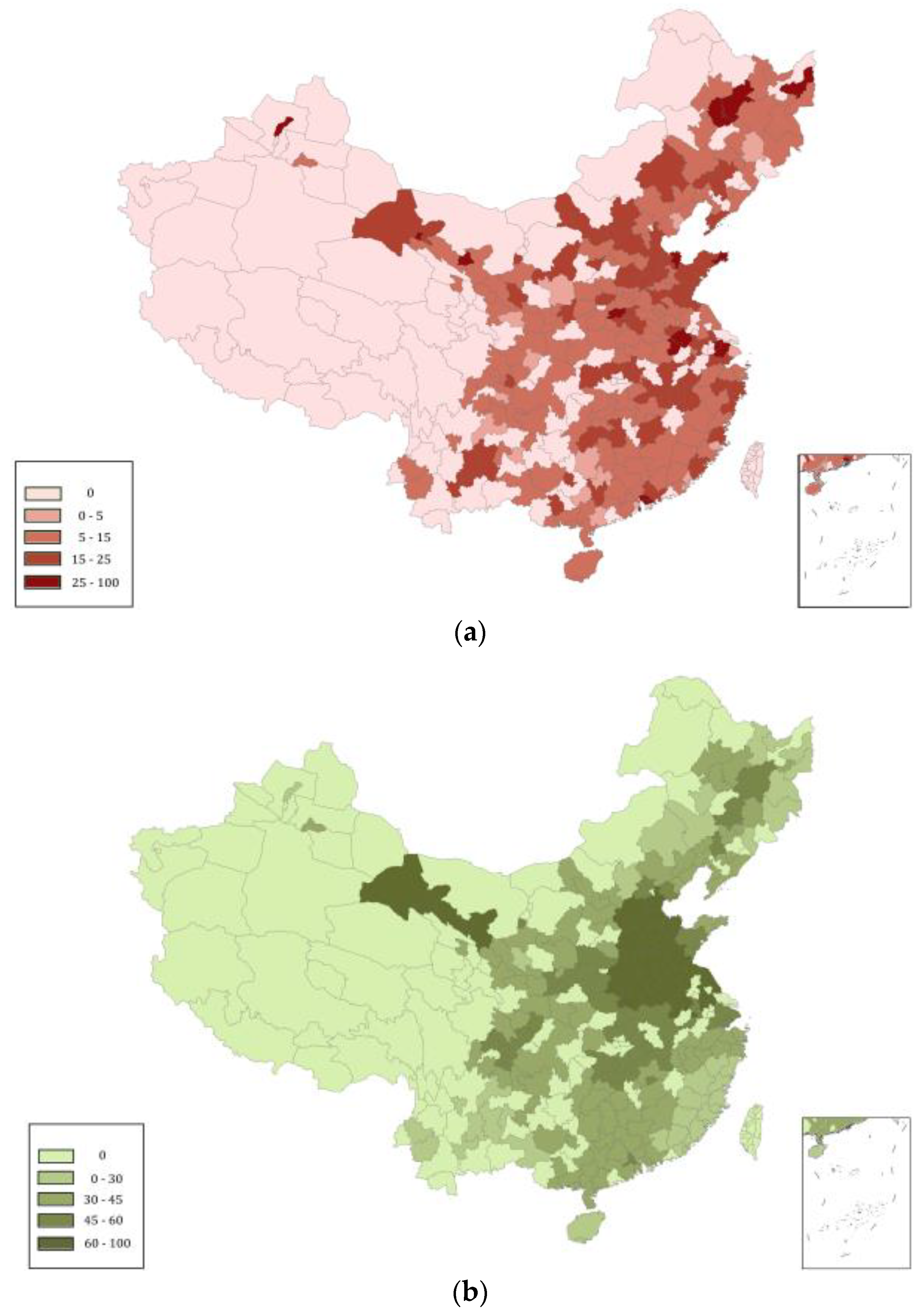
The main purpose of this paper is to study empirically the nonlinear relationship between transportation infrastructure construction and air quality using data from 280 prefecture-level cities in China from 2000 to 2017, finally advising China’s future transport policies and environmental dilemmas. This paper has the following three contributions. First, the Panel Smooth Transition Regression (PSTR) model was used to study the nonlinear effect of transportation infrastructure on air quality. This paper finds traffic infrastructure may have different effects on air pollution at different periods and regions. Additionally, there may be a nonlinear relationship between the two. At a low level of economic development, the impact of transportation infrastructure on air quality is different from that at a high level. Inspired by Sofien (2019) [26], this paper found that Panel Smooth Transition Regression (PSTR) could not only measure the threshold value of a variable, but also observe the size of the coefficient change over time [27]. In other words, it can calculate the specific value of the influence coefficient of transportation infrastructure on air quality in different periods. Second, the samples are divided into three sub-samples: eastern, central and western. China has a vast territory with distinct urban features. For example, there are significant differences in per capita income, number of vehicles, size of urban space, population density and meteorological environment, which all affect air quality [28]. To be specific, the overall economic development of the eastern region is more developed. The population density is higher as well as temperature and rainfall. The overall economic development of western China is relatively slow, with low population density, relatively low temperature and low rainfall. The central region is in the middle. The eastern region contains 106 cities, the central region contains 92 cities, and the western region contains 82 cities, as shown in Figure 2. The robustness of the results can be further verified by three sub-samples. The eastern regions include: Beijing, Tianjin, Hebei, Liaoning, Shanghai, Jiangsu, Zhejiang, Fujian, Guangdong, Shandong and Hainan. The central regions include: Henan, Shanxi, Inner Mongolia, Jilin, Heilongjiang, Anhui, Jiangxi, Hunan, Hubei and Guangxi. The western regions include: Sichuan, Guizhou, Yunnan, Xizang, Shaanxi, Gansu, Qinghai, Ningxia and Xinjiang. Third, the urban level can fully reflect the development status within China. The sample of this paper includes all the provinces and 280 prefecture-level cities from all provinces in China. Due to the diversity of cities and scales, the results of this paper are more targeted. In addition, urban built-up area is selected as the instrumental variable to overcome the endogeneity of the model to a certain extent.

The remainder of the paper is organized as follows. Section 2 establishes the empirical model; Section 3 shows the data source and variable selection process; Section 4 shows the data stationary test, nonlinearity test of panel model, determination of PSTR model conversion function and the number of position parameters, model estimation and result analysis; Section 5 describes the model endogeneity test, and Section 6 discusses conclusions and suggestions.

2. Methodology

In recent years, the superiority of nonlinear models in economic research has led many scholars to think that nonlinear models can more effectively describe the laws of economic changes. The nonlinear research on panel data mainly includes Threshold Regression (TR), Markov Regime Switching (MRS) and Smooth Transition Regression (STR) models, where the first two models assume that the conversion mechanism between variables is discrete, and this does not conform to the actual economic development laws. Based on the Panel Threshold Regression (PTR) model and STR, the scholars proposed the Panel Smooth Transition Regression (hereinafter referred to as PSTR) model which is mainly characterized by avoiding the mutability of the conversion mechanism [27]. This model describes the unique conversion gradualness of a variable in the panel data by means of a conversion function that transforms in the range from 0 to 1, which is more reasonable for an explanation of economic development.

The specific formula used in the PSTR model is:

$$y_{it}={\mu }_i+{\beta }_0^{\prime }{x}_{it}+{\beta }_1^{\prime }{x}_{it}g(q_{it};\gamma ,c)+u_{it}$$

(1)

$$i=1,\dots ,N,t=1,\dots T$$

where, $i$ represents the number of cross-sections, $t$ represents the length of time, $x_{it}$ is a k-dimensional explanatory variable, $y_{it}$ is the explained variable, ${\mu }_i$ and ${\mu }_{it}$ represent the individual fixed effect residuals and estimated residuals respectively. $g(q_{it};\gamma ,c)$ is a conversion variable with a value range from 0 to 1, which changes with the threshold variable; the regression coefficient is also dynamic, but between ${\beta }_0$ and ${\beta }_0+{\beta }_1$. Drawing on the research of Teräsvirta (1994) [28,29], this paper uses the logistic function as the conversion function. The specific function is shown in formula (2):

$$g(q_{it};\gamma ,c)={\left\{1+\exp \left[-\gamma {\displaystyle \prod _{j=1}^m(q_{it}-c_j)}\right]\right\}}^{-1}, \gamma >0,c_1\le c_2\le \dots \le c_m$$

(2)

In formula (2), $\gamma$ is the conversion rate and the slope parameter of the conversion function, which determines the speed and smoothness of the conversion mechanism, $q_{it}$ is a threshold variable, and $c=(c_1,c_2,\dots ,c_m)$ represents an m-dimensional vector of position parameters. $\gamma >0,c_1\le c_2\le \dots \le c_m$ is the limiting condition of the model. In actual economic research, the common parameters to be estimated can be met only by considering $m=1$ or $m=2$. When $m=1$, the model contains only one position parameter, and the conversion function increases monotonically with the change of $q_{it}$. When the conversion function tends to 0, the model is in the lower regime; when the conversion function tends to 1, the model is in the upper regime. When $q_{it}=c_j$, the conversion function takes a value of 0.5, and the model uses the position parameter as the symcenter to perform the mechanism conversion. At this time, the regression coefficient continuously changes between ${\beta }_0$ and ${\beta }_0+{\beta }_1$. When $m=2$, the conversion function takes the minimum value at $q_{it}=c_j$ and equals 1 when $q_{it}$ takes the minimum and maximum values, respectively. A multi-regime PSTR model will be obtained if the number of PSTR conversion functions is greater than 1:

$$y_{it}={\mu }_i+{\beta }_0^{\prime }{x}_{it}+{\displaystyle \sum _{j=1}^r{\beta }_j^{\prime }{x}_{it}{g}_j(q_{{}_{it}}^{\left(j\right)};{\gamma }_j,c_j)}+u_{it}$$

(3)

where the form of the conversion function $g_j(q_{it}^{(j)};{\gamma }_j,c_j)$ is the same as that of the logistic function in formula (2), and the model becomes an STR model of $r+1$ regime. The multi-regime conversion model as shown in formula (3) often appears as an alternative hypothesis to test whether the model is still nonlinear.

Since the number of conversion functions has not yet been determined, the fixed effect PSTR model equation is initially set as follows herein:

$$\ln {\mathrm{PM}}_{2.5}={\mu }_{it}+{\displaystyle \sum {\beta }_{it}\times x_{it}+}{\beta }_{it}^{\prime }g(\ln \mathrm{PGDP};{\gamma }_1,c_1)\times x_{it}+{\mu }_{it}$$

(4)

$$\ln {\mathrm{PM}}_{2.5}={\mu }_{it}+{\displaystyle \sum {\beta }_{it}\times x_{it}+}{\beta }_{it}^{\prime }g(\ln \mathrm{Car};{\gamma }_1,c_1)\times x_{it}+{\mu }_{it}$$

(5)

Formula (4) represents the model with GDP per capita (lnPGDP) as the conversion variable, and formula (5) represents the model with motor vehicle population per capita (lnCar) as the conversion variable. lnPM_2.5 represents the explained variable, $x_{it}$ represents the explanatory variable, ${\beta }_{it}$ is the estimated parameter of the linear part of the model, ${\beta }_{it}^{\prime }$ is the estimated parameter of the nonlinear part of the model, $q_{it}$ in Equation (2) is specifically the GDP per capita in Equation (4) and the motor vehicle in Equation (5), respectively. The remaining parameters have the same meaning as in formula (1). The final regression coefficient is between ${\beta }_{it}$ and ${\beta }_{it}+{\beta }_{it}^{\prime }$.

3. Variable Selection and Data Source

3.1. Explained Variable

At present, the data indicators for studying air pollution in China are divided into PM_2.5, API and AQI. However, API is only published until 2013, and involves only dozens of cities; AQI has been released since the end of 2013, and its length of time is relatively short. Therefore, this paper selects the PM_2.5 of air pollution in Chinese cities released by the Atmospheric Composition Analysis Groupof Dalhousie University, which involves a total of 280 prefecture-level cities. Compared to the first two, the data has an advantage in terms of time and samples of cit.

3.2. Explanatory Variable

Transportation infrastructure is generally reflected by the amount of urban road investment or road area. However, too much data on the amount of urban road investment is unavailable and part of the funds in urban road investment are used to upgrade roads or repair road damage. Only the increase in urban road area can really reduce traffic congestion and improve air quality, and the road area can also be used as a representative of the output of transportation infrastructure. Therefore, this paper selects the urban road area (lnRoad) as the core explanatory variable [9].

3.3. Conversion Variable

(1)

Urban GDP per capita (lnPGDP). GDP per capita can directly reflect the degree of regional economic development, and the economic development level directly determines the fiscal revenue of local governments as well as affecting the investment of environmental protection funds [30]. The classic EKC curve also indicates that there is an “inverted U” relationship between economic growth and environmental indicators, therefore, this paper selects GDP per capita as the conversion variable between transportation infrastructure and air pollution.

(2)

Urban motor vehicle population (lnCar). It is difficult to obtain urban traffic flow data, as the motor vehicle population can represent the degree of traffic congestion only to a certain extent. The living environment of residents has the self-repair capability, and will be damaged when the accumulated exhaust gas emitted by motor vehicles exceeds a certain amount, resulting in long-term deterioration of air quality [25]. In addition, the different numbers of motor vehicles represent different stages of development in the region. The greater number of motor vehicles indicates the higher level of economic development in the region [31]. Therefore, there may be a nonlinear relationship between motor vehicle population and environmental pollution. The motor vehicle population is selected as another conversion variable herein.

3.4. Control Variable

Based on the foregoing analysis and previous studies [7,9,18], this paper controls a group of urban characteristic variables in the empirical model to minimize the error due to missing variables. Specifically, the selection of urban characteristic control variables is explained below.

(1)

Urban population density (lnPD). Generally, air pollution is ascribed to human activities, and population aggregation will also affect air quality [32]. In this paper, the ratio of urban population to the area of regional administrative district is selected as the proxy variable of urban population density to control the impact of urban population agglomeration on air pollution.

(2)

Urban bus service (lnBus). Public transportation is regarded as an important way of green travel. The more developed public transportation is, the less frequently that private cars and taxis are used, thereby reducing exhaust emissions [33]. Herein, the number of buses per 10,000 persons in the city is used as a representative of urban public transportation.

(3)

Urban greening level (lnGreen). Green space absorbs carbon dioxide, which is conducive to purifying the air. Nonetheless, excessive investment in urban green space will occupy fiscal expenditures in environmental protection. The higher the value index of postmodernism is, the stronger the environmental awareness is, therefore, the more obvious the impact on air quality [21]. Hence, this paper introduces green space area per capita as a representative of urban greening level [34].

(4)

Environmental regulation (lnER). The government solves environmental problems by promulgating or implementing environmental policies, and environmental policies are also an important means to achieve green development and an environmentally-friendly society [16]. As a result, this paper uses the urban sewage treatment rate to control the intensity of the environmental regulations of the sample cities.

(5)

Urban natural climate factors. The natural climate conditions of a city will also affect its air quality [35]. The research found that the correlation between wind speed and PM_2.5 is significantly negative, as when the wind speed is low, the concentration of PM_2.5 does not change much. However, when the wind speed increases continuously, the concentration of PM_2.5 will decrease. The rainfall also has the obvious scour effect on natural air purification. Temperature had a positive correlation with PM_2.5 [36]. Thus, in this paper, urban precipitation (lnRain), urban wind speed (lnWind) and average temperature (lnTemp) are used to control the impact of different natural climate factors on air quality.

3.5. Instrumental Variable

Furthermore, this paper selects the built-up area (lnArea) as instrumental variables for testing endogeneity in discussion on missing variables. Air governance and urban construction are two key contents of local administration. It is difficult to maintain independence and exogeneity in the formulation of the two policies, as there may be a certain linkage; that is, air pollution has an impact on formulation of urban road policies. Such impact will cause the endogenous problem of reverse causality, leading to error in the parameter’s estimation results. In order to make the research results more reliable, this paper will use appropriate instrumental variables to control endogeneity. Appropriate instrumental variables must be related to endogenous variables and must remain exogenous to some extent; that is, such variables must be related to the road policies and unrelated to the missing variables. For different sample cities, the built-up area largely determines the shape and length of road construction, and the urban transportation infrastructure will also be affected by the built-up area [9]. As an inherent variable of geographic information, the built-up area will not change in a short period of time. Previous studies [37] have also selected this variable to describe the natural factors of cities.

Herein, the balanced panel data of 280 sample cities in the China City Statistical Yearbook from 2000 to 2017 are used for empirical research, and the average values of the successive two years are used to replace the missing data in individual years, with a total sample size of 5040. The PM_2.5 data is from the Atmospheric Composition Analysis Group of Dalhousie University, and has been updated from 2000 to 2017. Therefore, PM_2.5 takes the values in the years from 2000 to 2017. The urban road area is from the Wind database, and the natural factors such as urban annual precipitation, wind speed and average temperature are provided by the China Meteorological Data Sharing Service System. The rest of the data comes from the China City Statistical Yearbook and CEIC. All variables take the logarithms, and the data taking the logarithm are smoother to eliminate heteroscedasticity. The specific variable descriptions and data sources are shown in

Table 1. Variable meaning and statistical description.

Variable Name	Index	Variable Description	Obs	Mean	Std. Dev.	Min	Max	Data Resource
Independent Variable	lnPM2.5	PM2.5 index	5040	3.64	0.49	1.13	4.68	Atmospheric Composition Analysis Group
Dependent Variable	lnRoad	Road area per capita	5040	2.06	0.69	−1.97	4.69	Wind
Conversion Variable	lnPGDP	GDP per capita	5040	9.87	0.97	5.02	12.32	China City Statistical Yearbook and CEIC
	lnCar	Car ownership per capita	5040	5.98	1.13	2.10	9.70
Control Variable	lnBus	Buses per 10,000 people	5040	1.66	0.82	−1.35	4.75	China City Statistical Yearbook and CEIC
	lnPD	Population density	5040	6.56	0.95	3.64	9.09	China City Statistical Yearbook and CEIC
	lnGreen	Green area per capita	5040	1.91	1.12	−2.79	5.35	China City Statistical Yearbook and CEIC
	lnER	Environmental regulation	5040	4.42	0.27	1.22	4.61	China City Statistical Yearbook and CEIC
	lnRain	Average rain capacity	5040	987.78	570.53	42.40	3476	China Meteorological Science Data Sharing Network
	lnWind	Average wind speed	5040	2.13	0.81	0.20	6.90	China Meteorological Science Data Sharing Network
	lnTemp	Average temperature	5040	14.71	5.26	−5.00	25.40	China Meteorological Science Data Sharing Network
	lnArea	Construction land area	5040	4.22	0.87	1.53	7.28	China City Statistical Yearbook

, and the descriptive statistical results are shown in

Table 2. Unit root test.

Variables	LLC	IPS
lnPM2.5	−28.59 *** (0.00)	−2.89 *** (0.00)
lnRoad	−21.11 *** (0.00)	−2.14 *** (0.00)
lnPGDP	−12.76 *** (0.03)	−1.58 *** (0.01)
lnCar	−16.41 *** (0.00)	−1.87 *** (0.00)
lnBus	−14.61 *** (0.02)	−2.74 *** (0.00)
lnPD	−10.05 *** (0.01)	−4.75 *** (0.00)
lnGreen	−17.65 *** (0.00)	−2.09 *** (0.00)
lnER	−27.70 *** (0.00)	−2.57 *** (0.00)
lnRain	−34.17 *** (0.00)	−3.09 *** (0.00)
lnWind	−15.80 *** (0.00)	−1.66 ** (0.06)
lnTemp	−22.81 *** (0.00)	−2.18 *** (0.00)
lnArea	−7.59 ** (0.06)	−1.75 *** (0.00)

Note: *** and ** indicate significance at the levels of 1% and 5% respectively; the significance level for parameter estimates are in parentheses.

.

4. Empirical Results

4.1. Variable Stationary Test

Before constructing the model, we first need to perform a stationary test on each variable that takes a natural logarithm. After the Levin-Lin-Chu (LLC) test and the Im-Pesaran-Shin (IPS) test, all variables are stationary sequences, and the results are shown in Table 2. The null hypothesis of the stability test is that each interface sequence of panel data has the same unit root, and the alternative hypothesis is that each interface sequence has no unit root. It can be seen from the statistics and p-value results of the unit root test listed in Table 2, that the interface level values of various variables have no unit root. In addition, the results of Pedroni and Kao tests show that there is a cointegration relationship between explained variables and explanatory variables, that is, there is a long-term equilibrium relationship, and a panel model can be constructed.

4.2. Linearity and Nonlinearity Test

Before estimating the model parameters, we first need to perform a nonlinear test of the cross-sectional heterogeneity for the structural equation of air pollution. The null hypothesis H₀ of the test is that the panel data is a linear model that does not contain heterogeneity; the alternative hypothesis H₁ is the PSTR model containing at least one conversion function ($r\ge 1$). If the linear hypothesis of the model is rejected, then the number of conversion functions must be determined to ensure that the constructed PSTR model contains all nonlinear factors. This paper uses the LM (Equation (6)) and F-verion LM (Equation (7)) statistics used by Shao for testing [35].

$$LM=TN(SS{R}_0-SS{R}_1)/SS{R}_0~{\chi }^2(mk)$$

(6)

$$L{M}_F=[(SS{R}_0-SS{R}_1)/mk]/[SS{R}_0/TN-N-m(K+1)]~F(mk,TN-N-m(K+1))$$

(7)

where, SSR₀ and $SS{R}_1$ are the residual sum of squares estimated in the null hypothesis and alternative hypothesis models respectively, and the specific test results are shown in

Table 3. Nonlinear test and determination of conversion function purpose.

Model		H0:r = 0; H1:r = 1			H0:r = 1; H1:r = 2
		LM	LMF	LRT	LM	LMF	LRT
lnPGDP	Nation	674.81 (0.00)	30.67 (0.00)	727.76 (0.00)	261.66 (0.02)	32.40 (0.01)	269.12 (0.03)
	Eastern	439.32 (0.00)	22.46 (0.00)	503.56 (0.00)	42.07 (0.05)	4.99 (0.07)	42.56 (0.03)
	Central	226.24 (0.00)	10.20 (0.00)	244.38 (0.00)	31.82 (0.00)	3.76 (0.08)	32.15 (0.01)
	Western	154.80 (0.00)	6.70 (0.00)	164.09 (0.00)	31.86 (0.01)	1.87 (0.02)	32.23 (0.00)
lnRoad	Nation	647.20 (0.00)	29.21 (0.00)	695.65 (0.00)	220.58 (0.06)	27.07 (0.09)	225.85 (0.00)
	Eastern	428.68 (0.00)	21.75 (0.00)	489.54 (0.00)	72.64 (0.03)	8.78 (0.02)	74.15 (0.05)
	Central	187.32 (0.00)	8.21 (0.00)	199.52 (0.00)	30.37 (0.06)	3.59 (0.04)	30.67 (0.00)
	Western	144.04 (0.00)	6.18 (0.00)	152.04 (0.00)	18.66 (0.04)	2.18 (0.03)	18.78 (0.00)

.

This paper takes PM_2.5 as the explained variable and road area per capita as the explanatory variable. The GDP per capita and the car ownership per capita are used in turn as the conversion variables to perform the nonlinearity test of the panel data, and the test results are shown in Table 3. The second column H₀: r = 0 vs. H₁: r = 1 in Table 3 aims to test whether the model has nonlinearity. By observing the LM and LM_F statistic values and p-values, the results show that the models constructed by the two conversion variables have nonlinear characteristics. The variable that rejects the linearity most strongly should be selected as a conversion variable. The hypothesis in the third column, H₀: r = 1 vs. H₁: r = 2, is to test the number of model position parameters under the premise that there are nonlinear characteristics. In Table 3, lnPGDP and lnCar have large corresponding statistics of LM and LM_f, and the number of corresponding conversion functions r = 1, so the model is determined to be a two-regime model containing a conversion function; in addition, the AIC and BIC values when m = 1 are less than the test values when m = 2 for all models. Hence, the constructed model has a position parameter. The PSTR model allows the regression coefficients to change smoothly when moving from one “extreme” regime or state to another. In this paper, the influence of transportation infrastructure construction on air quality is divided into two stages, in which the coefficient will change greatly.

4.3. Explanation of GDP per Capita as a Conversion Variable

The PSTR model uses nonlinear least squares (NLS) to estimate the parameters. Before estimating the parameters, it is necessary to determine the initial values of the conversion rate and the position parameters first. Herein, the grid search method is used to determine its initial value [38]. In order to ensure the accuracy of the model estimation and the running time of the program at the same time, the number of iterations is initially set to 20,000, and the model parameter results are estimated, as shown in

Table 4. Parameter estimation results of GDP per capita model.

Variables	Nation	Eastern	Central	Western
lnRoad	0.06 *** (2.87)	0.14 *** (4.25)	0.25 *** (5.50)	0.01 * (1.89)
lnBus	−0.03 * (−1.65)	−0.04 * (−1.69)	0.13 ** (2.38)	0.01 (0.22)
lnPD	−0.06 *** (-3.91)	−0.07 *** (−3.04)	−0.28 *** (−3.80)	0.06 * (1.72)
lnGreen	−0.07 *** (−6.08)	−0.01 *** (−4.06)	0.01 (0.16)	−0.02 (−1.25)
lnER	0.013 (0.49)	−0.19 *** (−3.22)	−0.13 ** (−2.44)	0.06 (1.35)
lnRain	−0.058 *** (−2.82)	0.12 *** (3.37)	0.25 *** (5.41)	−0.10 *** (−3.99)
lnWind	−0.13 *** (−4.56)	−0.09 ** (−1.99)	0.06 (0.57)	−0.03 (−0.79)
lnTemp	0.48 *** (4.48)	0.33 *** (2.93)	0.34 *** (3.07)	−0.15 (−0.99)
lnRoad´	−0.05 ** (−2.04)	−0.17 *** (−3.91)	−0.18 *** (−3.72)	0.01 (0.40)
lnBus´	0.02 * (1.86)	0.03 (0.84)	−0.16 *** (−2.84)	−0.02 (−0.94)
lnPD´	0.03 ** (2.36)	0.10 *** (3.78)	−0.22 *** (-3.05)	−0.02 *** (−1.02)
lnGreen´	0.09 *** (7.03)	0.04 *** (1.86)	0.05 * (1.68)	0.01 (0.54)
lnER´	0.01 (0.15)	0.44 *** (6.17)	0.33 *** (5.25)	−0.07 * (−1.63)
lnRain´	0.05 ** (2.32)	−0.23 *** (−5.00)	−0.30 *** (−6.54)	0.07 *** (3.30)
lnWind´	0.13 *** (4.01)	0.14 ** (2.44)	−0.19 * (−1.89)	−0.03 (−0.71)
lnTemp´	−0.13 ** (−2.18)	−0.19 ** (−1.99)	−0.25 ** (−2.29)	0.05 (0.87)
${\gamma }_2$	2.74	1.29	37.50	18.85
$c_2$	8.88	9.39	8.59	6.05

Note: ***, **, and * indicate significance at the levels of 1%, 5%, and 10% respectively; the t-values for parameter estimates are in parentheses.

and

Table 5. Parameter estimation results of model of motor vehicle population per capita.

Variables	Nation	Eastern	Central	Western
lnRoad	0.30 *** (7.22)	0.10 *** (4.84)	0.15 *** (3.82)	0.09 * (1.68)
lnBus	−0.05 * (−1.79)	−0.02 ** (−1.90)	−0.01 * (−1.80)	−0.02 (−0.61)
lnPD	−0.19 *** (−6.58)	−0.05 *** (−2.84)	−0.16 *** (−5.00)	0.08 * (1.65)
lnGreen	−0.11 *** (−4.50)	0.04 *** (3.89)	0.07 *** (2.57)	−0.07 * (−1.76)
lnER	−0.06 (−0.82)	−0.06 (−1.53)	−0.15 *** (−2.52)	0.28 *** (3.47)
lnRain	−0.13 *** (−2.80)	0.05 *** (2.67)	0.16 *** (4.08)	−0.20 *** (−4.54)
lnWind	−0.29 *** (−4.87)	−0.01 (−0.54)	−0.18 ** (−2.97)	−0.03 (−0.37)
lnTemp	0.89 *** (5.30)	0.22 ** (2.42)	0.46 *** (4.04)	0.03 (0.20)
lnRoad’	−0.31 *** (−6.56)	−0.09 *** (−3.92)	−0.18 ** (−1.68)	−0.07 (−1.19)
lnBus´	−0.06 (−1.38)	−0.02 (−1.34)	−0.04 (−0.28)	0.03 (0.61)
lnPD´	0.19 *** (5.78)	0.05 *** (3.97)	0.34 *** (3.10)	−0.02 (−0.45)
lnGreen´	0.13 *** (4.63)	−0.02 * (−1.75)	−0.22 ** (−2.16)	0.05(1.37)
lnER´	0.13(1.21)	0.26 *** (7.58)	1.11 *** (4.24)	−0.28 *** (−3.36)
lnRain´	0.13 *** (2.52)	−0.14 *** (−6.20)	−0.57 *** (−3.43)	0.17 *** (4.03)
lnWind´	−0.33 *** (−4.67)	−0.04 * (−1.66)	−0.67 *** (−2.69)	−0.05 (−0.71)
lnTemp´	−0.65 *** (−4.02)	−0.14 *** (−3.11)	−1.37 *** (−3.45)	0.12 (1.17)
${\gamma }_2$	0.86	5.31	4.89	3.35
$c_2$	3.62	5.73	4.55	4.12

Note: ***, **, and * indicate significance at the levels of 1%, 5%, and 10% respectively; the t-values for parameter estimates are in parentheses.

.

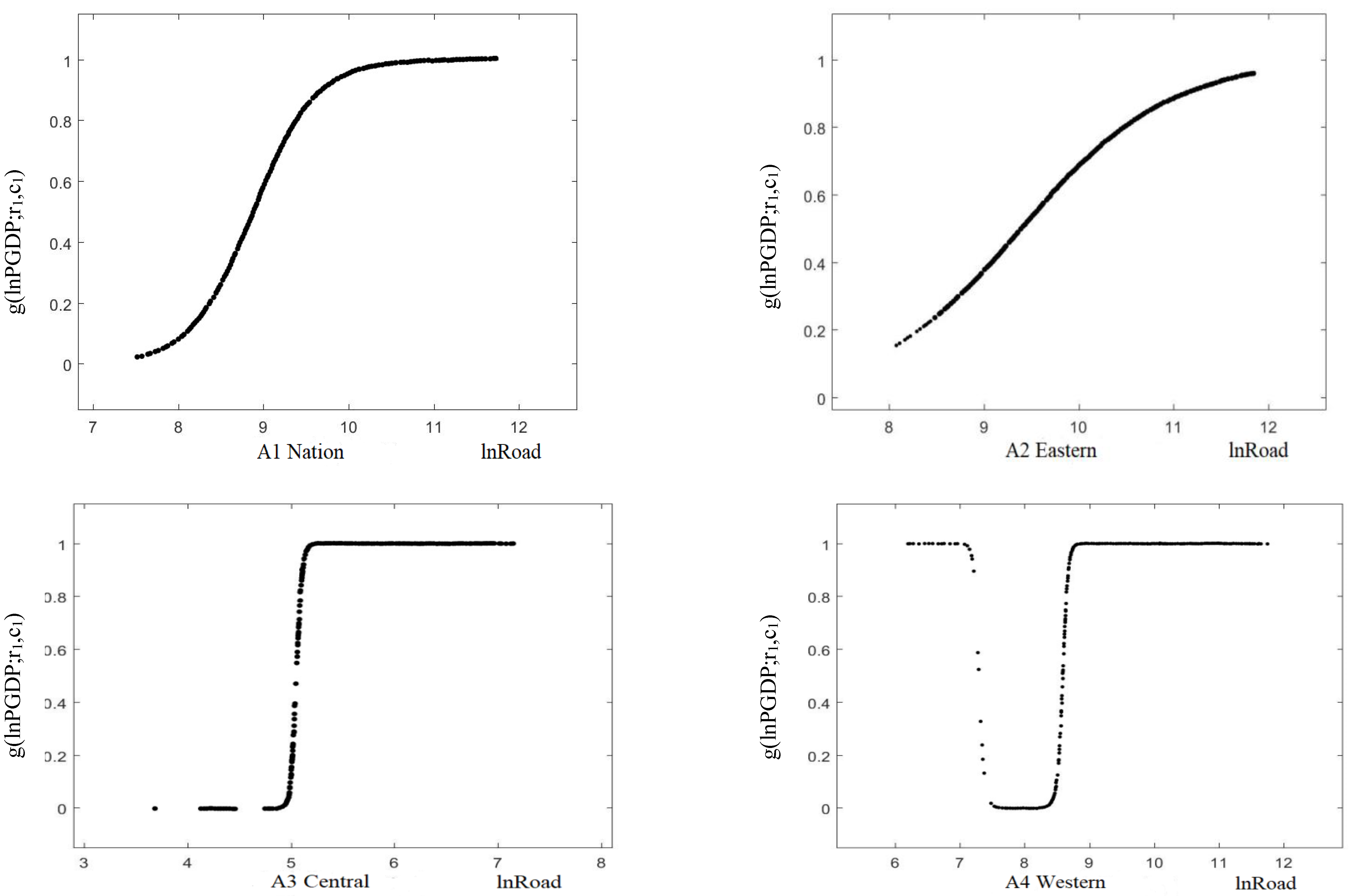
National samples: In the first column of Table 4, national city samples include a two-regime model of conversion variable in the model where the GDP per capita is a conversion variable. The estimated position parameter c of the model is 8.88, which is in the change range of the conversion variable. The conversion rate is 2.74. Only when the conversion slope $r$ approaches infinity, the two-regime model with m = 1 will become an indicator function, that is, (q > c) = 1. Otherwise it is 0. In other words, the PSTR model has not degenerated into Panel Transition Regression (PTR) model, so we believe that it is still necessary to explain the process of coefficient change with the idea of smooth transition. When the GDP per capita is greater than RMB exp (8.875) = 7151, the model gradually moves closer to the upper regime state with the increase of the conversion variable. When the GDP per capita is lower than RMB 7151, the model gradually falls back to the lower regime state as the conversion variable decreases. In the observed sequence of 5040 GDPs per capita, only 838 values are less than the position parameter, as shown by A1 in Figure 3. The curve indicates that the value of the conversion variable corresponds to the value of the conversion function, and the values following the position parameter are more intensive and significantly higher than the left parts of the position parameter. Therefore, most of the observations are above the position parameter, indicating that the model where the GDP per capita is the conversion variable is mainly in the upper regime range. In the lower regime state, the coefficient of road area per capita to air pollution in national city samples approaches 0.06; that is, when the road area per capita increases by 1%, the PM_2.5 index will increase by 0.06%. However, under the upper regime state, the coefficient of road area per capita to air pollution approaches −0.05; that is, when the road area per capita increases by 1%, the PM_2.5 index will decrease by 0.05%. In other words, the air pollution and economic development of the sample cities shows a positive correlation in the lower regime. Only when the GDP per capita is higher than a certain inflection point does the air pollution and economic development of the sample cities show a significant negative correlation in the upper regime, which also indirectly proved the EKC hypothesis. In addition, the coefficient of road area per capita to air pollution is positive in national city samples under the lower regime state; at this point, the corresponding GDP per capita is lower than RMB 7151. Under the upper regime state, such a coefficient is negative and the corresponding GDP per capita is higher than RMB 7151. It shows that people enjoy the convenience of life brought about by increased transportation infrastructure and also pay more attention to the welfare effect under the lower regime state, while they hate the environmental pollution caused by the traffic circulation and pay more attention to the environmental effect under the upper regime state. This is consistent with the results obtained by Yang (2018) [10]. The author found that urban transport investment will increase SO₂ emissions in the short term, but will reduce SO₂ emissions in the long term.

Regional samples: In the second column of Table 4, the position parameter is 9.39 and the conversion slope is 1.29 for the eastern city samples. In other words, when the GDP per capita is greater than RMB exp (9.39) = 11,908, the model gradually moves closer to the upper regime state with the increase of the conversion variable. If the GDP per capita is lower than RMB 11,908, the model gradually moves closer to the lower regime state. The coefficient of road area per capita to urban air pollution approaches 0.14 when the GDP per capita is in the lower regime state, while the estimated coefficient of road area per capita approaches −0.03 from positive to negative in the upper regime state. This shows that the correlation between road area per capita and air pollution is approaching −0.13 from 0.14, and the increase in road area has played a role in suppressing air pollution as the GDP per capita increases. Compared to other city samples, their conversion slope is the lowest. As can be seen from A2 in Figure 3, the slope of the curve is relatively gentle. In addition, in the 1908 eastern sample cities, only 371 values are lower than the position parameter, accounting for 19.45%. This indicates that a negative correlation is shown between the two, to a great extent.

In the third column of Table 4, the position parameter is 8.59 and the conversion slope is 37.50 for the central city samples. In other words, when the GDP per capita is greater than RMB exp (8.59) = 5394, the model will change from the lower regime state to the upper regime state. When the GDP per capita is lower than RMB 5394, the model will move closer to the lower regime state. The slope in the central region is the largest. As can be seen from A3 in Figure 3, the conversion trend is more intense. In the lower regime state, the coefficient of road area per capita to air pollution approaches 0.25, while the estimated coefficient approaches 0.07 (all are positive) in the upper regime state. In the upper regime state, the parameters are negative. Of the sample cities, 1536 are above the position parameter, accounting for 92.76% of the total sample. This indicates that a negative correlation is shown between the road area per capita and air pollution to a great extent in the central region.

In the fourth column of Table 4, the position parameter is 6.05 and the conversion slope is 18.85 for the western city samples. When the GDP per capita is greater than RMB exp (6.05) = 425, the model changes from the lower regime state to the upper regime state. As can be seen from A4 in Figure 3, the conversion slope in the western region is also larger. The coefficient of road area per capita to air pollution approaches 0.01 in the lower regime state, but approaches 0.02 in the upper regime state. In other words, the coefficient is always positive whether the model is in the lower or upper regime. However, the coefficient is not significant.

From the above analysis, the following can be found. First, for national, eastern and central sample cities, the coefficients of road area per capita to air pollution are significantly positive in the lower regime state and significantly negative in the upper regime state. Moreover, the sample cities in the upper regime state account for a large proportion, indicating that the increase in road investment is positively correlated to air pollution when the averages of GDP per capita of the whole nation, eastern region and central region are lower than RMB 29,135, RMB 37,609 and RMB 24,912, and negatively correlated to air pollution when such averages are higher than the above values. For western cities, the coefficients are significantly positive in the lower regime state, and negative but not significant in the upper regime state. Second, in terms of the degree of economic development, the degree of development and social welfare decreases sequentially in eastern, central and western regions, as do the conversion values of GDP per capita shown in Table 4, which can explain, to a certain extent, that people will pay more attention to the environmental effects of living conditions after the economy has developed to a certain stage. As people’s environmental values change, more and more attention is paid to the environment. Third, the conversion slope is gentle in the eastern region and steep in the central and western regions. The greater the conversion rate, the steeper the change of the conversion function value. This shows that the trend of suppressing air pollution will become more and more significant in the future as the GDP per capita further increases. Fourth, the reason why the coefficient of the western region is positive may be that this region is still in a stage for welfare effect, when people wish to improve the living standard by transportation infrastructure investments in view of the current development of the western region.

In terms of control variables, first, the coefficient of urban bus services in national city samples is −0.03 in the lower regime state and 0.02 in the upper regime state, indicating that the inhibitory effect of urban bus services on air pollution is weakening with the development of urbanization. However, the estimated coefficient of urban bus services is approaching −0.01, indicating that the improvement of urban bus services can significantly inhibit air pollution. The inhibitory effect of urban bus services on air pollution may be achieved by substitution effect of non-public transportation. In the future, it is necessary to further improve urban bus services, especially subways, intercity railways and other rail transit. Second, the population density changes from −0.06 in the lower regime state to 0.03 in the upper regime state, and the estimated coefficient is close to −0.03. The negative coefficient indicates that the increase in population density may force heavy pollution sources in the city to shift to the city’s boundary and remote areas, thereby improving the city’s internal air quality. Third, the estimated coefficient of green area is −0.07 in the lower regime state and 0.09 in the upper regime state, indicating that green area is conducive to reducing pollution in the early stage of urban development. However, in the middle and late stages, environmental pollution is much faster than green space purification. The estimated coefficient approaches 0.02. Fourth, in terms of natural factors, the estimated coefficient of average annual rainfall approaches −0.01, and the estimated coefficient of annual average wind speed in cities approaches −0.01, indicating that the average annual wind speed in cities will significantly affect the air quality of the sample cities. The faster wind speed and more rainfall are further conducive to the dissipation of atmospheric pollutants. The estimated coefficient of annual average temperature approaches 0.35, indicating that the temperature increase is not conducive to the dissipation of pollutants. The coefficients of environmental regulation are positive and not insignificant whether the model is in the lower or upper regime, indicating that the inhibitory effect of environmental regulations on air pollution has not been reflected. This paper aims to explore the structural impact of transportation infrastructure on air pollution. The remaining control variables are not key points and will not be detailed herein.

4.4. Explanation of Motor Vehicle Population per Capita as a Conversion Variable

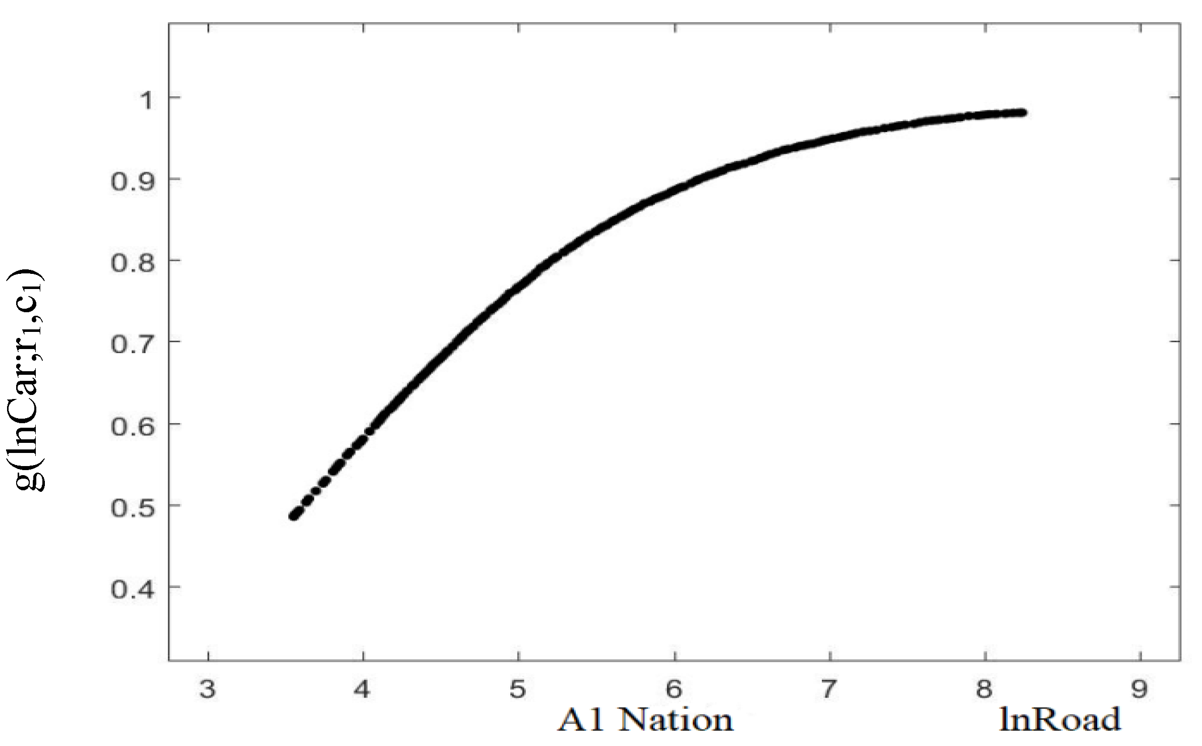
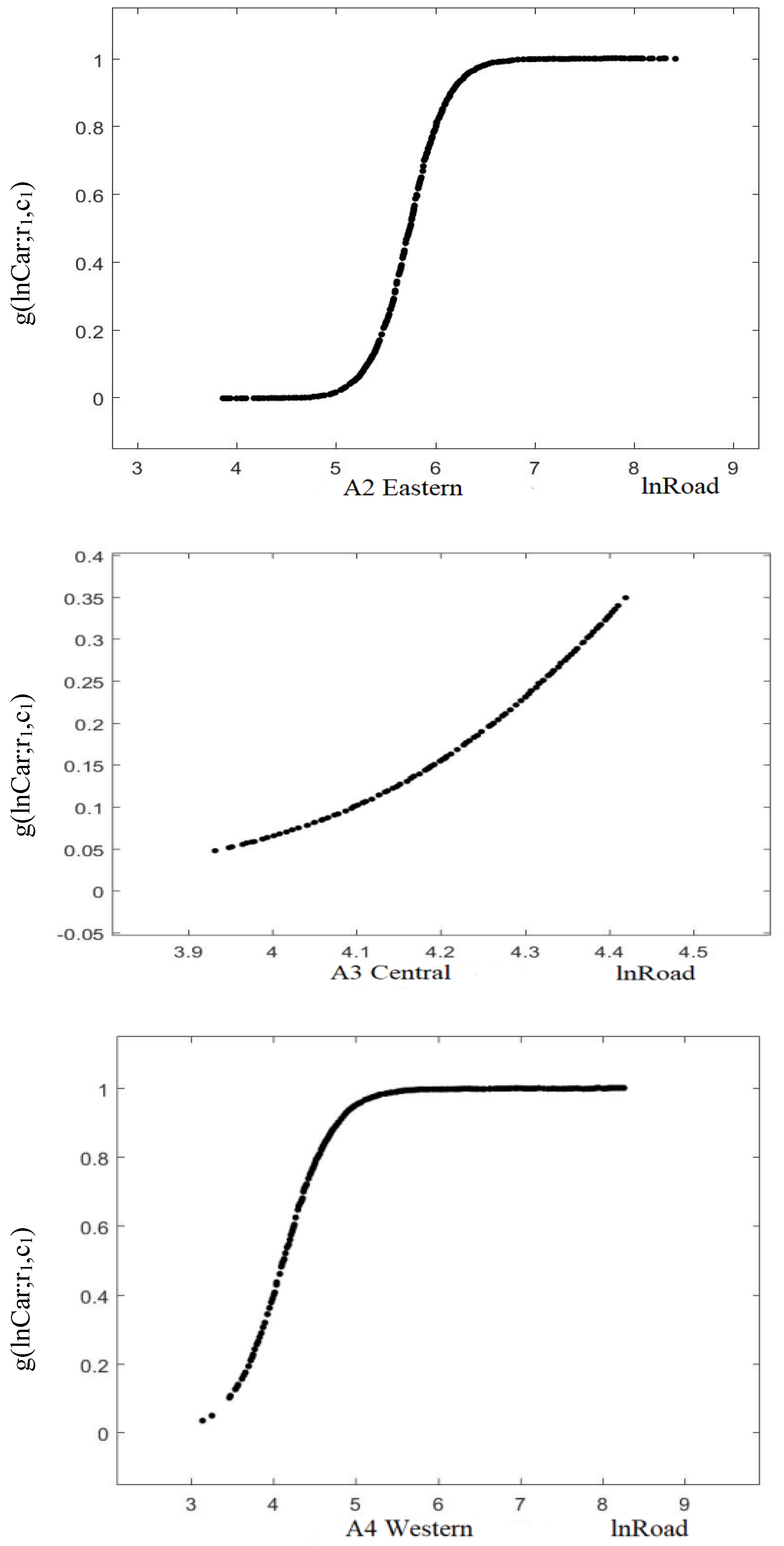
National city samples: In the first column of Table 5, national city samples include a two-regime model of conversion variable in the model where the motor vehicle population per capita is a conversion variable. The estimated position parameter of the model is 3.62, and the conversion slope is 0.86. That is, as the conversion variable increases, the model moves closer to the upper regime state when the motor vehicle population per capita is greater than exp (3.62) = 37 (vehicles/10,000 persons), and moves closer to the lower regime state when the motor vehicle population per capita is lower than 37. Relatively, the conversion rate is gentle, as shown by A1 in Figure 4. The coefficient of road area per capita also tends to −0.02 in the upper regime state from 0.30 in the lower regime state, indicating that every 1% increase in road area will reduce the degree of air pollution by 0.02% in the upper regime state. That the coefficient changes from positive to negative indicates that the inhibitory effect on air pollution will become more and more significant as the road area increases, even when the number of motor vehicles increases, which is proved by that the parameter 0.31 is greater than 0.30 in the upper regime state.

Regional samples: In the second column of Table 5, the position parameter is 5.73 and the conversion slope is 5.31 for the eastern city samples, and its conversion rate is the highest in the four models, as shown by A2 in Figure 4. In other words, the model moves closer to the upper regime state when the motor vehicle population per capita is greater than exp (5.31) = 309 (vehicles/10,000 persons), and moves closer to the lower regime state when the motor vehicle population per capita is lower than 309. The coefficient approaches 0.10 in the lower regime state and −0.01 in the upper regime state, indicating that the inhibitory effect on air pollution is significant.

In the third column of Table 5, the position parameter is 4.55 and the slope is 4.89 for the central region, as shown by A3 in Figure 4. That is, the model shifts to the upper regime state when the motor vehicle population per capita is greater than exp (4.89) = 94 (vehicles/10,000 persons), and moves closer to the lower regime state when the motor vehicle population per capita is lower than 94. The coefficient of road area per capita to air pollution tends to be 0.15 when the motor vehicle population per capita is in the lower regime and −0.03 when the motor vehicle population per capita is in the upper regime. That the coefficient changes from positive to negative also indicates that it has an inhibitory effect on air pollution. Parameter -0.18 in the upper regime is greater than the parameter in the lower regime, which also shows that the inhibitory effect will become more and more powerful.

In the fourth column of Table 5, the position parameter is 4.12 and the slope is 3.35 for the western city samples, as shown by A4 in Figure 4. That is, the model shifts to the upper regime state when the motor vehicle population per capita is greater than exp (3.35) = 29 (vehicles/10,000 persons), and moves closer to the lower regime state when the motor vehicle population per capita is lower than 28.62. The coefficient change from positive to negative indicates that the road area per capita is negatively correlated to air pollution. The control variables are basically in line with expectations. Only some of the variables in the western region are not significant enough. The control variables have the same meanings as those given in Table 4. They are not key points of this paper and will not be detailed herein.

As shown in Table 5, the coefficients are positive and significant in the lower regime state, and negative and significant in the upper regime state for national, eastern, central and western sample cities, indicating that the road investment is positively correlated to air pollution when the motor vehicle population per capita is below 37, 309, 94 and 29, and negatively correlated to air pollution when the motor vehicle population per capita is above 37, 309, 94 and 29. The motor vehicle population can reflect the wealth level of a region, which also shows that people pay more attention to the convenience of life brought by transportation investment and enjoy the welfare effects brought by life in the early stage of economic development, but hate the environmental pollution caused by transportation investment and pay more attention to environmental effect at a certain stage of economic development.

By comparing Table 4 with Table 5, it can be found that it does not matter if the GDP per capita or motor vehicle population per capita is used as the conversion variable, the relationship between road area per capita and air pollution is positive in the lower regime state, and negative in the upper regime state, and the coefficient changes from positive to negative. In other words, it does not matter if taking the GDP per capita or the motor vehicle population per capita is used as the conversion variable, as with the development of economy and the increase of wealth, the increase of road area per capita has a stronger and stronger inhibitory effect on air pollution. This result is similar to that found by Sun [39], that transportation infrastructure construction can significantly alleviate pollution in the long term, but not in the short term. Secondly, through the comparison between Figure 3 and Figure 4, it can be found that the conversion slope of each region is different; the ranking order of the conversion slope is the central region, western region, eastern region and the whole nation in the model with GDP per capita as the conversion variable from large to small, while the eastern region, central region, western region and the whole nation in the model with motor vehicle population as the conversion variable. Although there are differences, on the whole, the slope of the eastern region is much higher than that of the central and western regions, indicating that with the passage of time, the environmental governance effect of the eastern region is much higher than that of the central and western regions.

5. Robustness Test

Considering the regression results of the benchmark model are likely to be endogenous, this paper adds the built-up area (lnArea) as instrumental variables. The rationality of instrumental variables has been explained in the variable description of the previous article [37,38], and the test results are shown in

Table 6. Endogenous test results of model with GDP per capita as a conversion variable.

Variables	Nation	Eastern	Central	Western
lnArea	0.51 *** (2.99)	−0.31 ** (−2.06)	0.42 ** (3.10)	0.26 ** (2.43)
lnRoad	0.11 * (1.81)	0.16 *** (3.06)	0.22 ** (2.31)	−0.11 (−0.11)
lnBus	0.01 (1.07)	−0.02 * (−2.02)	0.21 (1.20)	0.01 (0.60)
lnPD	−0.19 ** (−2.35)	−0.15 ** (−2.57)	−0.52 *** (−4.80)	0.11 (0.58)
lnGreen	0.03 * (1.90)	0.04 (0.99)	−0.13 (−0.81)	−0.11 (−1.90)
lnER	−0.23 * (−1.88)	−0.21 *** (−5.12)	−0.10 ** (−2.10)	0.12 (0.89)
lnRain	−0.03 (−1.31)	−0.17 *** (−4.36)	0.23 *** (4.01)	−0.30 (−1.61)
lnWind	−0.18 *** (−3.99)	−0.11 ** (−2.43)	0.03 (0.45)	0.01 (0.70)
lnTemp	0.39 *** (5.01)	0.40 * (1.99)	0.31 ** (2.51)	0.43 ** (2.45)
lnArea´	−1.89 *** (−5.21)	−0.34 *** (−5.39)	−1.40 *** (−2.40)	−0.35 * (−2.86)
lnRoad´	−0.20 ** (−2.01)	−0.14 * (−1.89)	−0.31 *** (−2.82)	0.08 (0.41)
lnBus´	−0.32 (−1.08)	−0.10 * (−1.89)	−0.75 (−1.61)	−0.31 (−1.38)
lnPD´	0.12 ** (1.89)	0.10 ** (2.33)	0.82 *** (2.86)	0.45 ** (2.51)
lnGreen´	0.32 ** (2.51)	−0.03 (−1.16)	0.41 (1.21)	0.21 (1.31)
lnER´	0.29 *** (5.21)	0.35 *** (6.20)	0.30 *** (4.06)	−0.02 (−0.89)
lnRain´	−0.31 *** (−3.51)	−0.32 *** (−6.62)	−0.10 *** (−5.40)	0.12 * (1.89)
lnWind´	0.36 *** (5.61)	0.19 ** (2.40)	−0.26 (−1.10)	0.11 (0.21)
lnTemp´	−0.16 (−1.04)	−0.09 (−0.09)	−0.11 (−0.67)	0.21 * (1.86)
${\gamma }_2$	2.81	1.79	2.33	4.25
$c_2$	10.39	9.99	5.19	8.99

Note: ***, **, and * indicate significance at the levels of 1%, 5%, and 10% respectively; the t-values for parameter estimates are in parentheses.

and

Table 7. Endogenous test results of model with motor vehicle population per capita as a conversion variable.

Variables	Nation	Eastern	Central	Western
lnArea	0.36 ** (2.31)	−0.31 ** (−2.05)	0.81 *** (6.60)	0.21 * (1.88)
lnRoad	0.04 *** (5.91)	0.06 ** (2.32)	0.26 *** (6.30)	0.25 ** (2.41)
lnBus	0.01 ** (2.35)	0.01 * (1.79)	0.01 (0.89)	0.11 (1.56)
lnPD	−0.05 ** (−2.33)	−0.03 * (−1.89)	−0.07 * (−1.88)	0.25 (0.35)
lnGreen	−0.01 (−0.51)	0.21 ** (2.39)	−0.06 (−1.12)	−0.11 ** (−2.36)
lnER	−0.04 ** (−2.45)	−0.33 *** (−4.12)	0.01 (1.36)	−0.12 (−1.01)
lnRain	−0.11 (−0.58)	0.07 *** (3.51)	−0.19 (−1.43)	−0.02 (−1.03)
lnWind	−0.07 *** (−4.40)	−0.11 * (−1.87)	−0.10 *** (−3.26)	−0.03 (−0.77)
lnTemp	0.36 *** (6.19)	0.11 (0.99)	0.36 *** (3.40)	0.41 (1.01)
lnArea´	−0.06 ** (−2.04)	−0.81 *** (−3.21)	−0.51 ** (−2.45)	−0.29 *** (−3.32)
lnRoad´	−0.19 *** (−4.00)	−0.20 (−1.45)	−0.21 ** (−2.31)	−0.29 ** (−1.90)
lnBus´	−0.30 (−1.52)	−0.01 * (−1.77)	−0.09 ** (−2.33)	−0.16 (−1.51)
lnPD´	0.03 *** (3.38)	0.01 * (1.91)	0.09 *** (3.79)	0.41 ** (2.51)
lnGreen´	0.03 *** (2.91)	0.01 (0.55)	0.06 ** (2.35)	0.12 *** (3.26)
lnER´	0.21 ** (2.36)	0.30 * (1.86)	0.20 ** (2.35)	0.81 (1.33)
lnRain´	−0.11 (−0.29)	−0.23 *** (−6.85)	−0.12 ** (−1.89)	0.31 (1.07)
lnWind´	−0.22 *** (−5.50)	−0.14 * (−1.51)	0.26 ** (2.21)	0.20 * (1.89)
lnTemp´	−0.09 ** (−1.99)	−0.36 (−0.89)	−0.31 *** (−5.88)	0.17 (0.55)
${\gamma }_2$	3.02	4.48	2.77	1.26
$c_2$	6.76	5.86	6.56	6.30

Note: ***, **, and * indicate significance at the levels of 1%, 5%, and 10% respectively; the t-values for parameter estimates are in parentheses.

.

The results of endogenous test with GDP per capita as the conversion variable are shown in Table 6, which respectively shows the regression results of the national, eastern, central and western city samples. The results show that, except for the western region, the coefficient of urban road area to air pollution is still significantly positive in the lower regime, and is still significantly negative in the upper regime, which verifies the improvement effect of urban traffic infrastructure on air quality; that is to say, increasing urban road area will significantly inhibit urban pollution. The coefficients of other control variables are similar to those in Table 4, indicating that the main conclusions of this paper are robust.

The results of endogenous test with motor vehicle population per capita as the conversion variable are shown in Table 7, which respectively shows the regression results of the national, eastern, central and western city samples. The results show that the coefficient of urban road area to air pollution is still significantly positive in the lower regime, and is still significantly negative in the upper regime, which verifies the improvement effect of urban traffic infrastructure on air quality; that is to say, increasing urban road area will significantly inhibit urban pollution. The coefficients of other control variables are similar to those in Table 5, indicating that the main conclusions of this paper are robust.

6. Conclusion and Policy Implications

6.1. Conclusion

In China, since the deterioration of air quality has seriously harmed the health of residents and the improvement of social welfare, the government has also raised environmental governance to an unprecedented level. Although vehicle emission has become a major contributor of pollution to urban environment [39], it is more important to increase investment in road traffic infrastructure in the context that alternative fuels and new energy technologies are still not widely used. Based on 280 prefecture-level cities in China from 2000 to 2017, this paper studies the impact of urban transportation infrastructure on air quality. Considering that this impact is nonlinear, it is based on PSTR model, GDP per capita and motor vehicle population per capita respectively, as conversion variables for empirical analysis. In addition, considering possible endogeneity between traffic infrastructure and air quality, and in order to further verify the robustness of the model, this paper adds the one-period lag of air quality and the built-up area as instrumental variables to the model respectively. The main conclusions of this paper are as follows.

First, the results of the model with GDP per capita as the conversion variable show that when GDP per capita is less than 7151, the impact of transportation infrastructure investment on air quality is positive, which indicates that in this stage of development, people pay more attention to the convenience of life brought by transportation infrastructure investment and enjoy the welfare of economic development; and that in the development state of GDP per capita greater than 7151, the impact of transportation infrastructure investment on air quality is negative, which indicates that at this stage of development, people pay more attention to the surrounding living environment and have higher requirements for environmental improvement. According to the characteristics of economic development, the overall sample of Chinese cities is divided into three sub-samples: the eastern region, the central region and the western region. The sub-samples are similar to the whole sample in the empirical results. The eastern cities, the central cities and the western cities all show the characteristics of positive in the low development stage and negative in the high development stage, but the conversion values of each region are different, which are 11,908, 5394 and 22,917 in the eastern region, the central region and the western region respectively. Second, the results of the model with motor vehicle population per capita as the conversion variable show a similar rule; that is, it is positive in the low development stage, and negative in the high development stage. The conversion values of the whole nation, the eastern region, the central region and the western region are 37, 309, 94 and 28 respectively. The results of the two models show that increasing road area will be in favor of reducing air pollution in the future. Third, urban public transport services, green area and population density are all conducive to reducing air pollution, and the natural environment of the regions, such as wind speed and rainfall, will also reduce the emission of pollutants. However, the role of environmental regulation is not significant, which may be due to the tendency of local governments to protect local economic development at the expense of environment in the process of implementing regional environmental regulation. Fourth, after adding two instrumental variables of air quality lag item and built-up area, the conclusion of negative correlation between road area and air quality is further strengthened.

6.2. Policy Implications

The above empirical results have brought us some policy implications, and different regions should put forward development strategies that suit them “according to local conditions”. The specific recommendations are as follows: First, as an economically developed region in China, the eastern region should further accelerate the improvement and upgrading of urban transportation infrastructure. Relative to the increasing number of motor vehicles and their emissions, the expansion and reconstruction of road facilities, the optimal layout of transportation networks, and traffic management are all very important. Measures to build new road facilities, widen the main roads of the old cities, as well as optimize and improve the operational efficiency of traffic roads are currently required by most cities. Second, the economic development of the central and western regions is relatively slow. Considering that its construction requires large capital and time costs, it is difficult to take effect in the short term. It may be considered to increase the transportation capacity of existing facilities and increase transportation efficiency while expanding capacity as well as improve the transportation efficiency of the transportation infrastructure by increasing the passenger load and loading rate. Third, while increasing traffic capacity, rationally optimizing road facilities and road planning, vigorously developing intelligent transportation systems, rationally arranging pedestrians, non-motor vehicles, and motor lanes, as well as strengthening public transportation management law enforcement and traffic law publicity can effectively improve road capacity.

The focus of this study is on the impact of transportation infrastructure on air quality, without considering air pollution from other sources. For example, some cities will have thermal power plants, which is also one of the sources of air pollution. How to distinguish air pollution caused by traffic from other sources of pollution is the next research direction. In addition, whether the empirical conclusions obtained in this paper are general requires empirical testing worldwide.

References

- Giovanis, E. The relationship between teleworking, traffic and air pollution. Atmos. Pollut. Res. 2018, 9, 1–14. [Google Scholar] [CrossRef] [Green Version]
- Wróbel, A.; Rokita, E.; Maenhaut, W. Transport of traffic-related aerosols in urban areas. Sci. Total Environ. 2000, 257, 199–211. [Google Scholar] [CrossRef]
- Mao, R.; Duan, H.; Dong, D. Quantification of carbon footprint of urban roads via life cycle assessment: Case study of a megacity- Shenzhen, China. J. Clean. Prod. 2017, 166, 40–48. [Google Scholar] [CrossRef]
- Wheeler, A.J.; Smith-Doiron, M.; Xu, X. Intra-urban variability of air pollution in Windsor, Ontario-measurement and modelling for human exposure. Environ. Res. 2008, 106, 7–16. [Google Scholar] [CrossRef]
- Luo, Z.; Wan, G.; Wang, C.; Xun, Z. Urban pollution and road infrastructure: A case study of China. China Econ. Rev. 2018, 49, 171–183. [Google Scholar] [CrossRef]
- Sun, D.; Zeng, S.X.; Han, L.; Meng, X.H. Can transportation infrastructure pave a green way? A city-level examination in China. J. Clean. Prod. 2019, 226, 669–678. [Google Scholar]
- Chen, Y.; Whalley, A. Green infrastructure: The effects of urban rail transit on air quality. Am. Econ. J. 2012, 4, 58–97. [Google Scholar] [CrossRef] [Green Version]
- Bel, G.; Holst, M. Evaluation of the impact of bus rapid transit on air pollution in Mexico city. Transp. Policy 2018, 63, 209–220. [Google Scholar] [CrossRef]
- Sun, C.W.; Zhang, W.Y.; Fang, X.M.; Gao, X.; Xu, M.L. Urban public transport and air quality: Empirical study of China cities. Energy Policy 2019, 135, 1–9. [Google Scholar]
- Zheng, S.; Kahn, M.E. Understanding China’s urban pollution dynamics. J. Econ. Lit. 2013, 51, 731–772. [Google Scholar] [CrossRef] [Green Version]
- Vickrey, W.S. Congestion theory and transport investment. Am. Econ. Rev. 1969, 59, 251–260. [Google Scholar]
- Beirão, G.; Cabral, J.A.S. Understanding attitudes towards public transport and private car: A qualitative study. Transp. Policy 2007, 14, 478–489. [Google Scholar] [CrossRef]
- Börjesson, M.; Hamilton, C.J.; Näsman, P. Factors driving public support for road congestion reduction policies: Congestion charging, free public transport and more roads in Stockholm, Helsinki and Lyon. Transp. Res. Part A Policy Pract. 2015, 78, 452–462. [Google Scholar] [CrossRef]
- Duran-Fernandez, R.; Santos, G. Road infrastructure spillovers on the manufacturing sector in Mexico. Res. Transp. Econ. 2014, 46, 17–29. [Google Scholar] [CrossRef]
- Tao, L.; Wenyue, Y.; Haoran, Z.; Xiaoshu, C. Evaluating the impact of transport investment on the efficiency of regional integrated transport systems in China. Transp. Policy 2016, 45, 66–76. [Google Scholar]
- Yang, M.; Ma, T.; Sun, C. Evaluating the impact of urban traffic investment on SO2 emissions in China cities. Energy Policy 2018, 113, 20–27. [Google Scholar] [CrossRef]
- Chen, X.; Shao, S.; Tian, Z.; Xie, Z.; Yin, P. Impacts of air pollution and its spatial spillover effect on public health based on China’s big data sample. J. Clean. Prod. 2017, 14, 915–925. [Google Scholar] [CrossRef]
- Guttikunda, S.K.; Goel, R.; Pant, P. Nature of air pollution, emission sources, and management in the Indian cities. Atmos. Environ. 2014, 95, 501–510. [Google Scholar] [CrossRef]
- Ahmad, F.; Mahmud, S.A.; Yousaf, F.Z. Shortest processing time scheduling to reduce traffic congestion in dense urban areas. IEEE Trans. Syst. Man Cybern. Syst. 2016, 47, 838–855. [Google Scholar] [CrossRef]
- Duggal, V.G.; Saltzman, C.; Klein, L.R. Infrastructure and productivity: A nonlinear approach. J. Econom. 1999, 92, 47–74. [Google Scholar] [CrossRef]
- De las Heras-Rosas, C.J.; Herrera, J. Towards sustainable mobility through a change in values. Evidence in 12 European Countries. Sustainability 2019, 11, 4274. [Google Scholar] [CrossRef] [Green Version]
- Chen, X.; Huang, B.; Lin, C.T. Environmental awareness and environmental Kuznets curve. Econ. Model. 2019, 77, 2–11. [Google Scholar] [CrossRef]
- Bi, C.; Jia, M.; Zeng, J. Nonlinear effect of public infrastructure on energy intensity in China: A panel smooth transition regression approach. Sustainability 2019, 11, 629. [Google Scholar] [CrossRef] [Green Version]
- Wang, C.; Ming, K.L.; Zhang, X.Y.; Zhao, L.F.; Paul, T.W.L. Railway and road infrastructure in the Belt and Road Initiative countries: Estimating the impact of transport infrastructure on economic growth. Transp. Res. Part A Policy Pract. 2020, 134, 288–307. [Google Scholar] [CrossRef]
- Fu, S.; Gu, Y. Highway Toll and Air Pollution: Evidence from Chinese Cities. J. Environ. Econ. Manag. 2017, 83, 32–49. [Google Scholar] [CrossRef] [Green Version]
- Tiba, S. Modeling the nexus between resources abundance and economic growth: An overview from the PSTR model. Resour. Policy 2019, 64, 1–8. [Google Scholar] [CrossRef]
- González, A.; Teräsvirta, T.; Dijk, D. Panel Smooth Transition Regression Models; SSE/EFI Working Paper Series in Economics and Finance; Stockholm School of Economics: Stockholm, Sweden, 2005. [Google Scholar]
- Bertolini, L.; Clercq, F.L. Urban development without more mobility by car? Lessons from Amsterdam, a multimodal urban region. Environ. Plan. A 2003, 35, 575–589. [Google Scholar] [CrossRef]
- Teräsvirta, T. Specification, estimation, and evaluation of smooth transition autoregressive models. J. Am. Stat. Assoc. 1994, 89, 208–218. [Google Scholar]
- Shao, S.; Tian, Z.; Fan, M. Do the rich have stronger willingness to pay for environmental protection? New evidence from a survey in China. World Dev. 2018, 105, 83–94. [Google Scholar] [CrossRef]
- Teik, H.L.; Hussain, H.; Chia, N.G. The motorcycle to passenger car ownership ratio and economic growth: A cross-country analysis. J. Transp. Geogr. 2015, 46, 122–128. [Google Scholar]
- Vikas, S.; Ranjeet, S.S.; Jaakko, K. An approach to predict population exposure to ambient air PM2.5 concentrations and its dependence on population activity for the megacity London. Environ. Pollut. 2020, 257, 1–12. [Google Scholar]
- Lu, H.; Zhu, Y.; Qi, Y.; Yu, J. Do Urban Subway Openings Reduce PM2.5 Concentrations? Evidence from China. Sustainability 2018, 10, 4147. [Google Scholar] [CrossRef] [Green Version]
- Sun, C.; Zhang, W.; Luo, Y.; Xu, Y. The improvement and substitution effect of transportation infrastructure on air quality an empirical evidence from China’s rail transit construction. Energy Policy 2019, 129, 949–957. [Google Scholar] [CrossRef]
- Tétreault, L.F.; Eluru, N.; Hatzopoulou, M.; Morency, P.; Plante, C.; Morency, C.; Reynaud, F.; Shekarrizfard, M.; Shamsunnahar, Y.; FaghihImani, A.; et al. Estimating the health benefits of planned public transit investments in Montreal. Environ. Res. 2018, 160, 412–419. [Google Scholar] [CrossRef] [PubMed]
- Cao, R.; Li, B.; Wang, Z.Y. Using a distributed air sensor network to investigate the spatiotemporal patterns of PM2.5 concentrations. Environ. Pollut. 2020, 264, 114–126. [Google Scholar] [CrossRef] [PubMed]
- Aslanidis, N.; Xepapadeas, A. Regime switching and the shape of the emission—Income relationship. Econ. Model. 2008, 25, 731–739. [Google Scholar] [CrossRef]
- Wang, S.; Li, W.; Dincer, H.; Yuksel, S. Recognitive approach to the energy policies and investments in renewable energy resources via the fuzzy hybrid models. Energies 2019, 12, 4536. [Google Scholar] [CrossRef] [Green Version]
- Sun, C.W.; Yuan, L.; Li, J.L. Urban traffic infrastructure investment and air pollution: Evidence from the 83 cities in China. J. Clean. Prod. 2018, 172, 488–496. [Google Scholar] [CrossRef]
Figure 1.
Number of motor vehicles and road area.
Figure 2.
The annual average of distinct urban features in different regions in 2017 (a) PM2.5 index; (b) Urban road area per capita (square meter).
Figure 3.
Conversion function of GDP per capita model.
Figure 4.
Conversion function of model of motor vehicle population per capita.