Identifying Seasonal Accumulation of Soil Salinity with Three-Dimensional Mapping—A Case Study in Cold and Semiarid Irrigated Fields

Abstract

Soil salinity is an active and complex part of soil property in arid and semiarid irrigation areas that restricts the sustainability of agriculture production. Knowledge of seasonal distributions and migration of soil salinity is important for the management of agriculture. In this study, three-dimensional (3-D) geostatistical methods were used to construct seasonal 3-D spatial distribution maps of soil salinity, and then the quantitative analysis methods were used to study the seasonal accumulation patterns of soil salinity for the 0–150 cm soil depth in cold and semiarid irrigated rice fields. The results revealed that there were different spatial distribution and migration patterns of soil salinity in autumn 2015, spring 2016, autumn 2016, and spring 2017. The migration of soil salinity had a dispersion trend from autumn to spring, and the area of non-saline soil increased. Whereas there was an accumulation trend from spring to autumn, and the area of non-saline soil decreased. There were about 10–20% of the study area had experienced transitional changes of different soil salinity levels in different seasons. The correlation coefficient showed that there were significant positive correlations among the five depth increments (30 cm) in different seasons, and the correlations of soil salinity were higher in adjacent layers than in nonadjacent layers. The EC_e values were higher in the topsoil (0–30 cm) and deeper subsoil (120–150 cm), indicating that soil soluble salts accumulated in the soil surface due to evaporation and accumulated in the bottom due to leaching and drainage. Microtopography was the major factor influencing spatial distribution of soil salinity in different seasons. The EC_e values were generally higher in the swales or in areas with rather poor drainage, whereas the values were lower in relatively higher-lying slopes or that were well-drained. The results provide theoretical basis and reference for studying the variation of seasonal soil salinity in irrigated fields.

1. Introduction

Soil salinity is one of the major threats to plant growth and agricultural production, as it is highly possible that soil salinity leads to land degradation, soil fertility decline, and crop productivity decreases, particularly in areas that are used for irrigated agriculture [1,2]. The growth of crops in these areas may be threatened by overirrigation, poor quality irrigation water, salt–laden groundwater, and insufficient drainage [3]. If the internal drainage of soil profiles is insufficient to drain the salt that is brought in with irrigation water, soluble salt accumulated through natural salinization processes and human activities may have great damage to soil [4]. Statistics have shown that approximately 20% of irrigated agriculture worldwide is affected by salt, and this proportion is increasing because of high evaporation, low rainfall, inadequate irrigation and other irrational anthropogenic activities [5,6].

Soluble salt can be caused by environmental factors (e.g., geological, hydrological, and topographic) or unreasonable and disordered human activities (e.g., overirrigation and land use change) [7]. Irrigation water dissolves native salt and transfers them to soil, resulting in the increase of soil salt content [8]. Soil texture and soil layering configurations impact salt migration during the infiltration and evaporation processes, which increase the risk of salinization and sodification in the root zone and decrease the yields of crop [9]. Although soil salinity is widely gaining attention, it has considerable variability on both spatial and temporal scales due to the heterogeneity of the soil profile and unreasonable irrigation systems and cultivation modes [10]. To assess and manage salinization or desalinization, as well as to prevent land degradation, one must monitor and quantify changes in soil salinity over space and time [11].

The spatial and temporal variability of soil salinity is one of the most important areas in soil science, and it is the foundation for studying the sources of salinization, the amelioration of saline soil, and the assessments of farmland sustainability [12,13,14]. Thus, geostatistical techniques that estimate values at unsampled locations are widely applicable for studying the spatial structure of soil salinization and its consequences for classifying and surveying an area [15]. In most soil surveys, the required soil property information is often obtained from transects. However, soil sediments are complicated, and the properties can vary greatly in the horizontal and vertical directions. To obtain the lateral and vertical variation characteristics of soil salinity, three-dimensional (3-D) geostatistical methods are needed to describe and map the 3-D spatial distribution of soil salinity. Recently, many studies have concentrated on the three-dimensional geostatistical methods to study the 3-D distributions of soil properties, such as soil texture, soil carbon storage, and soil salinity [16,17,18,19]. The intention of 3-D geostatistical methods are modeling the semivariograms in the 3-D direction, thus, 3-D geostatistical methods can effectively describe and visualize the whole soil profile and complement the deficiency of prediction accuracy in the study of the vertical stratification by two-dimensional (2-D) geostatistical methods [20,21].

In irrigated agricultural areas, seasonal variations of soil salinity, as well as its horizontal and vertical variations, are complicated processes due to the water application patterns and strong evaporation, as well as human activities. It is important for land evaluation, improvement, and the sustainable development of agricultural production to construct the 3-D spatio–temporal of soil salinity for the soil profile by seasonal soil surveys. In this study, the Ili River Valley, a typical cold and semi-arid irrigated agricultural region in China, is used as a case study to provide quantitative information for the management of seasonal soil drainage and salt leaching with the application of 3-D geostatistical methods. The intention of the research were (1) to map the seasonal 3-D variations and distribution of soil salinity based on the 3-D mesh model; (2) to quantify seasonal changes in the soil salinity status in the horizontal and vertical directions by comparing datasets collected in spring and autumn; (3) to assess the influence of different water sources on seasonal accumulation of soil salinity; and (4) to propose some suggestions for the sustainable management of soil water and salt.

2. Materials and Methods

2.1. Study Site

The study area is located on the Northern slope of the Tianshan Mountains, Xinjiang, China (Figure 1), which is the main rice-producing area of Xinjiang. The sampling area is located in the middle of Qapqal County (longitude 81°8′55″–81°17′10″ E, latitude 43°45′55″–43°49′35″ N), where two rivers flow. The climate of the area is temperate continental, with cold winters and hot summers; the temperature in summer (from June to August) is generally 22.6–33.5 °C, and the average temperature in winter (from November to March) is −9.4 °C. The average annual precipitation is 222 mm, the average annual evaporation is 1549.9 mm, and the average annual snow depth is 200–300 mm. The study area is a mixed zone of river terrace and inclined plain. The elevation ranges from 612 to 675 m, and it increases from northwest to southeast. After years of agricultural development, a fine soil layer has been formed in the study area. The zonal soil is mainly composed of loam, and the bottom of the soil (90–150 cm) is the mixture of loam, silt loam, and sandy loam. The dominant land use type is cropland, and irrigation is the main water source. The irrigation period for rice is May–September, and the freezing–thawing period for fields is December–March.

2.2. Soil Sampling and Laboratory Analysis

To investigate seasonal spatial distribution characteristics of soil salinity, 210 measurement points were arranged in autumn (28 October–30 October) 2015, spring (19 April–21 April) 2016, autumn (30 October–1 November) 2016, and spring (25 April–27 April) 2017, respectively. The soil was sampled in a pseudoregular grid (0.5 km × 0.5 km), which was determined based on the distribution pattern of cropland in the study area. At each site, an intact soil core was sampled at the depths of 0–30, 30–60, 60–90, 90–120, and 120–150 cm, and the coordinates of the sampling site was recorded by portable Global Positioning System (GPS). All the soil samples were air-dried, crashed, and passed through a 2 mm sieve for further analysis. A total of 250 g of treated soil was mixed with water to make into a saturated paste [22]. The saturated paste was left untouched for up to 12 h, then using the method presented in Rhoades (1996) to measure the electrical conductivity of the saturation extract (EC_e, dS m⁻¹) [12,23].

2.3. Geostatistical Analysis and Mapping Methods

The spatial variability in soil properties is mostly studied using geostatistical methods. A semivariogram is the basis for geostatistical methods and a tool that shows spatial correlations among data [24]. The basis of the semivariance function is the expectation that, on average, the values of adjacent samples are more similarly than those are nonadjacent [25]. In general, the equation is as follows:

$$\gamma (h)=\frac{1}{2N(h)}{\displaystyle \sum _{i=1}^{N(h)}{[z(x_i)-z(x_i+h)]}^2}$$

(1)

where h is the spacing of the sample points; γ(h) is the semivariogram value; N(h) is the number of pairs with the spacing of h; z(x_i) is the measured value of sample point x_i; and z(x_i + h) is the measured value of the sample point (x_i + h). Then the estimated value can be calculated as follows:

$$z(x_0)={\displaystyle \sum _{i=1}^n{\lambda }_{i}z(x_i)}$$

(2)

where z(x₀) is the estimated value of location x₀; n is the number of sites for the estimate within the search neighborhood; and λ_i is the weight of the ith observation.

In 3-D spatial interpolation, the implication is that a variable is spatially sampled in 3-D to allow for the modeling of 3-D directional semivariograms [21]. In general, the 3-D directional semivariograms were modeled by combining the horizontal and vertical direction into a 3-D structure [26]. Groundwater Modeling System (GMS) software was used to build a 3-D scatter data model map for different soil layers [27]. If there were strong spatial autocorrelation for the scatter data, a 3-D mesh model (Figure 2b) can be built to structure the 3-D scatter data (Figure 2a). Finally, the GMS software was used to interpolate 3-D data with kriging interpolation method on the basis of 3-D mesh model (Figure 2c).

2.4. Statistical Evaluation

Two different criteria were used to validate the model: The root mean squared error (RMSE) and coefficient of determination (R²). The formulas are as follows:

$$RMSE=\sqrt{\frac{1}{N}{\displaystyle \sum _{i=1}^N{[z^{*}(s_i)-z(s_i)]}^2}}$$

(3)

$$R^2=\frac{{\left[{\displaystyle {\sum }_{i=1}^N\left(z(s_i)-z{(s_i)}_{ave}\right)\left(z^{*}(s_i)-z^{*}{(s_i)}_{ave}\right)}\right]}^2}{{\displaystyle {\sum }_{i=1}^N{\left(z(s_i)-z{(s_i)}_{ave}\right)}^2{\displaystyle {\sum }_{i=1}^N{\left(z^{*}(s_i)-z^{*}{(s_i)}_{ave}\right)}^2}}}$$

(4)

where z^*(s_i) and z(s_i) are the simulated and measured values, respectively; z^*(s_i)_ave and z(s_i)_ave are the average simulated and measured values, respectively; and N is the number of observations. The best fit between the simulated and measured values under ideal conditions would be RMSE = 0 and R² = 1.

3. Results

3.1. 3-D Analyses of Soil Samples

Using the GMS software, we obtained 3-D scatter data model maps of 210 noncontiguous sample points for the five depth increments (0–30, 30–60, 60–90, 90–120 and 120–150 cm) in autumn 2015, spring 2016, autumn 2016, and spring 2017 (Figure 3), and they were used as the basis for the maps of the 3-D mesh model and the 3-D distribution of soil EC_e. To obtain better visualizations, all 3-D maps were expanded approximately 1500 times in the vertical direction.

Pearson correlation analyses were conducted on soil salinity for the five depth increments in autumn 2015, spring 2016, autumn 2016, and spring 2017, respectively (

Table 1. Pearson correlation coefficients between the EC_e values at different depths (i.e., 0–30, 30–60, 60–90, 90–120, 120–150, and 0–150 cm) in autumn 2015, spring 2016, autumn 2016, and spring 2017.

Depth (cm)	Autumn 2015					Spring 2016
	0–30	30–60	60–90	90–120	120–150	0–30	30–60	60–90	90–120	120–150
0–30	1					1
30–60	0.923 *	1				0.931 *	1
60–90	0.851 *	0.922 *	1			0.870 *	0.893 *	1
90–120	0.836 *	0.877 *	0.941 *	1		0.922 *	0.913 *	0.901 *	1
120–150	0.834 *	0.883 *	0.911 *	0.927 *	1	0.912 *	0.878 *	0.882 *	0.911 *	1
Depth (cm)	Autumn 2016					Spring 2017
	0–30	30–60	60–90	90–120	120–150	0–30	30–60	60–90	90–120	120–150
0–30	1					1
30–60	0.932 *	1				0.899 *	1
60–90	0.907 *	0.917 *	1			0.826 *	0.899 *	1
90–120	0.869 *	0.863 *	0.938 *	1		0.900 *	0.910 *	0.942 *	1
120–150	0.906 *	0.851 *	0.925 *	0.912 *	1	0.785 *	0.885 *	0.881 *	0.915 *	1

Note: * represents significant correlation (p < 0.01).

). The results showed that the soil EC_e values among the five different depths were significantly positively correlated, and two adjacent soil layers were more closely correlated than nonadjacent layers. The seasonal correlation coefficients ranged from 0.834 to 0.941, 0.870 to 0.931, 0.851 to 0.938, and 0.785 to 0.942, respectively, and reached a significance correlation level (p < 0.01), indicating high correlations of the soil salinity factors at the five depth increments in different seasons.

3.2. Descriptive Statistics and Geostatistical Analysis of Soil Salinity

Summary statistics of the average soil salinity (EC_e) for the 0–150 cm soil depth were shown in

Table 2. Descriptive statistics of the average soil EC_e for the 0–150 cm soil depth in autumn 2015, spring 2016, autumn 2016, and spring 2017. K–S test: Kolmogorov–Smirnov test.

Time	Sample Size	Max.	Min.	Average	Standard Deviation	CV (%)	Skewness	Kurtosis	K–S Test
Autumn 2015	210	7.99	0.65	2.26	1.80	80	1.26	1.35	0.31
Spring 2016	210	7.32	0.53	1.90	1.56	82	1.67	1.99	0.21
Autumn 2016	210	7.57	0.63	2.57	1.95	76	0.89	0.58	0.60
Spring 2017	210	6.94	0.51	1.96	1.39	71	1.75	2.45	0.47

. The corresponding ranges of soil salinity were 0.65–7.99, 0.53–7.32, 0.63–7.57, and 0.51–6.94 dS m⁻¹ in autumn 2015, spring 2016, autumn 2016, and spring 2017, respectively; and the average soil salinity in autumn (2.26 and 2.57 dS m⁻¹, respectively) was higher than in spring (1.90 and 1.96 dS m⁻¹, respectively, Table 2). The values of coefficient of variation (CV) were 71–82%, indicating that seasonal soil salinity for the 0–150 cm soil depth had moderate variations. The Kolmogorov–Smirnov (K–S) test showed that soil salinity conformed to normal distribution in different seasons, indicating that the data were suitable for the geostatistical analysis.

Table 3. Semivariogram parameters and prediction errors of the average soil EC_e for the 0–150 cm soil depth in autumn 2015, spring 2016, autumn 2016, and spring 2017. RMSE: root mean squared error.

Time	Model	C0	C0 + C	C0/(C0 + C)	Range (km)	RMSE	R2
Autumn 2015	Gaussian	1.612	6.509	0.248	0.667	1.427	0.748
Spring 2016	Gaussian	0.243	4.110	0.059	0.476	1.073	0.808
Autumn 2016	Gaussian	1.320	5.604	0.236	0.420	1.260	0.817
Spring 2017	Gaussian	0.529	4.266	0.124	0.714	0.975	0.795

presented the fitted theoretical models of semivariance of the average soil EC_e for the 0–150 cm soil depth in autumn 2015, spring 2016, autumn 2016, and spring 2017. Regarding the spatial prediction of soil EC_e, the R² values ranged from 0.748 to 0.817, and the RMSE values ranged from 0.975 to 1.427, demonstrating that the spatial maps of soil salinity estimated by ordinary kriging interpolation were reliable and acceptable. The parameters of R² and RMSE showed that the Gaussian models well described the spatial pattern of the average soil EC_e for the 0–150 cm soil depth. The nugget to sill ratio (C₀/(C₀ + C)) is usually used to classify the spatial dependence of regional variables. In general, when the ratio is less than 0.25, there is strong spatial dependence; the ratio is between 0.25 and 0.75, there is moderate spatial dependence; otherwise, there is weak spatial dependence and it is not suitable for spatial interpolation [28,29]. As indicated in Table 3, the nugget to sill ratio (C₀/(C₀ + C)) of different seasons were 0.248, 0.059, 0.236, and 0.124, which were less than 0.25 in the different seasons, suggesting strong spatial autocorrelation for soil salinity in the irrigated field. The comprehensive analysis indicated that it was suitable to use the spatial interpolation method for the prediction analysis of the 0–150 cm soil depth.

3.3. Seasonal 3-D Variations of Soil Salinity

To conduct 3-D spatial interpolation, the 3-D mesh model of the study area was built with the 3-D scatter data by using the GMS software (Figure 2). Then, the GMS software was used to create 3-D spatial distribution maps of soil salinity with the kriging interpolation method on the basis of 3-D scatter data and 3-D mesh model. In general, the levels of agricultural soil salinity (i.e., EC_e, dS m⁻¹) were classified as: Non-saline (0–2 dS m⁻¹), slightly saline (2–4 dS m⁻¹), moderately saline (4–8 dS m⁻¹), strongly saline (8–16 dS m⁻¹), and extremely saline (>16 dS m⁻¹) [1]. According to the FAO (1976), the yields of rice can be reduced by approximately 25% when the EC_e value is 6 dS m⁻¹ [30]. In addition, there was no extremely saline soil (>16 dS m⁻¹) in the study area. Therefore, the levels of soil salinity in this study were classified as: 0–2, 2–4, 4–6, 6–8, and >8 dS m⁻¹.

Data collection over multiple seasons provided a seasonal time-lapse series of 3-D images for the entire 0–150 cm soil depth (Figure 4). Soil salinity generally decreased from southwest to northeast in the study area, with a higher soil salinity in the west and a lower soil salinity in the north. Overall, the spatial distribution of the EC_e pattern remained similar from autumn (autumn 2015 and 2016) to spring (spring 2016 and 2017), which showed that the migration of soil salinity from autumn to spring was small. However, the spatial distribution of the EC_e pattern was different from spring 2016 to autumn 2016. There was a considerable change in the distribution of soil salinity, which indicated a large migration from spring to autumn.

Non-saline soil (0–2 dS m⁻¹) was the main type in the study area, however, saline soil (i.e., slightly, moderately, and strongly saline, >2 dS m⁻¹) was also present and should not be ignored. Figure 5 showed the area statistics of different soil salinity levels in autumn 2015, spring 2016, autumn 2016, and spring 2017. The areas of different soil salinity level have considerable changes in different seasons. Approximately 10% of the study area experienced transitional changes of different soil salinity levels from autumn 2015 to spring 2016, and approximately 19% experienced transitional changes from autumn 2016 to spring 2017. Compared to the autumn seasons of 2015 and 2016, the area of non-saline soil (0–2 dS m⁻¹) increased, and the area of saline soil (>2 dS m⁻¹) decreased in the spring seasons of 2016 and 2017, indicating a dispersion trend. There was also a considerable change in soil salinity from spring to autumn. Approximately 17% of the study area experienced transitional changes of different soil salinity levels from spring 2016 to autumn 2016. Compared to spring 2016, the area of non-saline soil (0–2 dS m⁻¹) decreased, and the area of saline soil (>2 dS m⁻¹) increased in autumn 2016, indicating an accumulation trend.

3.4. Seasonal Distribution of Soil Salinity in the Vertical Direction.

Based on the spatial distribution maps of soil salinity, six typical cross-sections were created by the GMS software (with a spacing of 2.25 km from north to south and 3.5 km from east to west). These six typical sections were labeled A, B, C, D, E, and F, and the specific locations of the six sections are shown in Figure 6. Two types of textural profiles could be distinguished: One type was homogeneous and had a low soil salt content (<2 dS m⁻¹), and there were marked changes in the soil salt content of the other type at different depths (Figure 6).

To investigate the profile distributions of soil EC_e in different seasons, the soil layers were divided into five depths ranges (0–30, 30–60, 60–90, 90–120, and 120–150 cm). The box plots in Figure 7 allowed us to compare the changes in soil EC_e at different depths and times. As shown in Figure 7, the average EC_e values decreased for the 0–60 cm soil depth and increased for the 60–150 cm soil depth in the vertical variations, which indicated a trend that soil salinity accumulated in the topsoil (0–30 cm) and deeper subsoil (120–150 cm). For seasonal variation of soil EC_e, as shown in Figure 7, the average soil EC_e for different soil layers decreased from autumn to spring, while it increased from spring to autumn. These results indicated that seasonal migration mechanism of soil salinity are differences in the vertical, and there is a dispersion trend of soil salinity from autumn to spring and an accumulation trend from spring to autumn.

4. Discussion

4.1. Spatial Variation of Soil Salinity

Soil salinity mainly originate from the weathering, accumulation of irrigation water–salt, and deposition of salty dust [31]. In irrigated agricultural regions, environmental factors and human activities can directly affect the movement and exchange of soluble salt and salt ions in soil solutions [32]. At large spatiotemporal scales, environmental factors, such as hydrological processes, topography, and climate conditions, result in high soil salt contents [33]. At small spatiotemporal scales, microtopography and human activities, such as irrigation networks and the changes of land use, mainly determine soil salinity variation [34].

In the study area, the random factors, such as rice production methods, land use, and climate change, were stable and had low influences on the accumulation of soil salinity in the short term. The geostatistical analyses showed that structural factors, such as hydrological conditions and topography, were the primary factors affecting the spatial autocorrelation of soil salinity (C₀/(C₀+C) < 0.25, Table 3). Since seasonal hydrological processes differ in cold and semiarid irrigated fields, the seasonal migration of soil salt differs. Our data suggested that there was a dispersion trend of soil salinity from autumn to spring and an accumulation trend from spring to autumn, and there were about 10–20% of the study area had experienced transitional changes of soil salinity in different seasons (Figure 4 and Figure 5). To manage seasonal soil water and salt better, it is vital to understand the migration processes of soil salinity in the horizontal and vertical directions. Therefore, two main factors that control salinization, hydrological processes and topography, were selected to explore their effects on the distribution and migration of soil salinity in the study area.

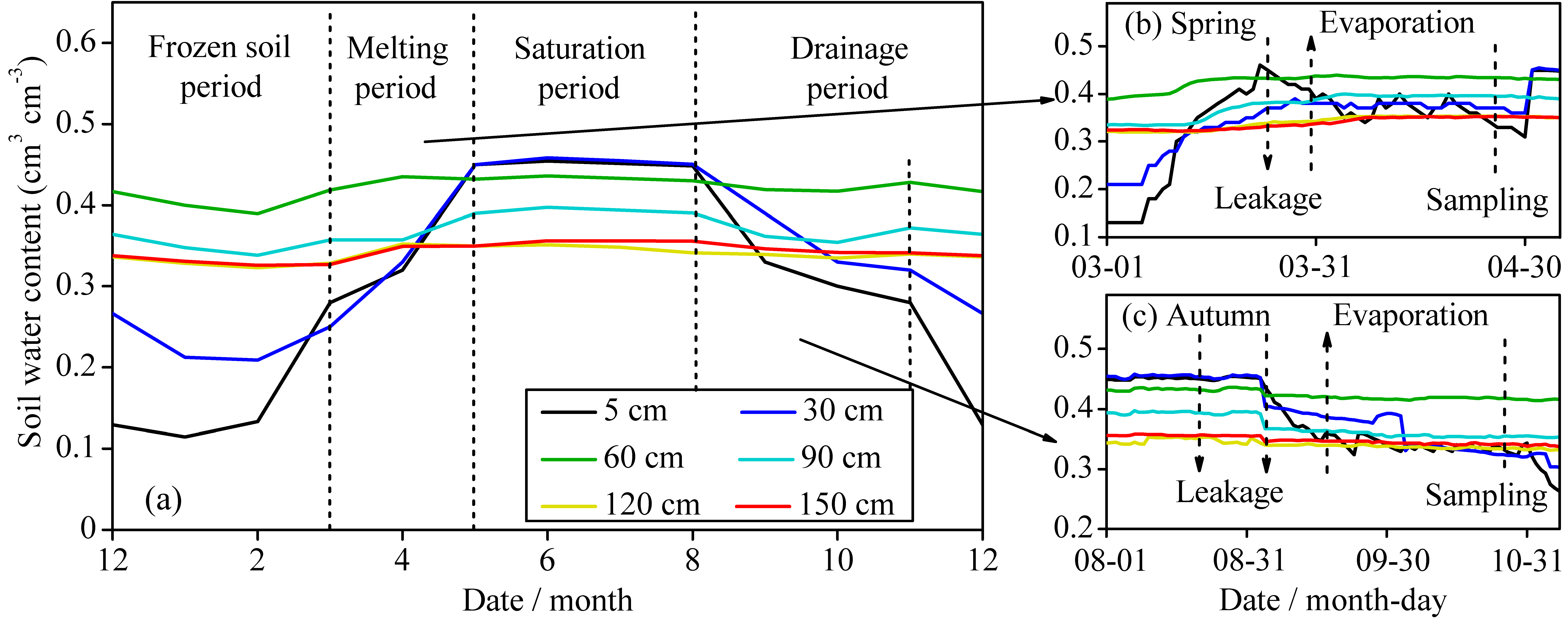
4.2. Effects of Hydrological Processes on Soil Salinity

In irrigated agricultural regions, water is the key driver influencing the migration of soil salinity [35]. All factors related to hydrological processes, such as irrigation or other water sources that inflow and outflow, affect the distribution and migration of soil salinity in the horizontal and vertical direction [36,37]. There were two main hydrological processes in the study area: The freezing–thawing process of snow cover from winter to spring, and the irrigation process from summer to autumn (Figure 8a, measured by Hydraprobe meter, USA). The freezing–thawing process of snow cover occurred within a relatively short time and redistributes soil salinity in spring. As shown in Figure 8a, the average soil water content for the 0–150 cm soil depth declined continuously from November to March of the following year, and the transport of soluble salt to the soil surface was limited due to the low evaporation, which resulted in downward leaching and the drainage of soil soluble salt during these periods. The soil water content increased from March to April due to the snow thawing process (Figure 8b). However, the amount of surface snowmelt runoff was limited and the duration was short, resulting in a relatively small impact on large-scale salt migration. Therefore, there was only a small area migration of soil salinity from autumn to spring (Figure 4). In addition, there is a dispersion trend of soil salinity from autumn to spring due to leaching and water drainage, and soil salinity in vertical profiles was generally lower than that in autumn.

Water inflows mainly occurred via irrigation water (e.g., snowmelt water and groundwater from the mountains, Cl⁻–Na⁺ type) from spring to autumn, resulting in the raising of the water table with continued irrigation. As shown in Figure 8a, the average soil water content for the 0–150 cm soil depth was nearly saturated from May to August. The migration of water and salt were governed by regional vertical and lateral drainage flows, which resulted in an accumulation trend from spring to autumn (Figure 4). The soil water content and water table declined due to the termination of irrigation during the rice harvest period (Figure 8c). Soil soluble salt accumulated in the soil surface due to high evaporation and accumulated in the deeper subsoil due to leaching and drainage. As a result, the EC_e values were lower in the subsoil (60–90 cm) and higher in the topsoil (0–30 cm) and deeper subsoil (120–150 cm).

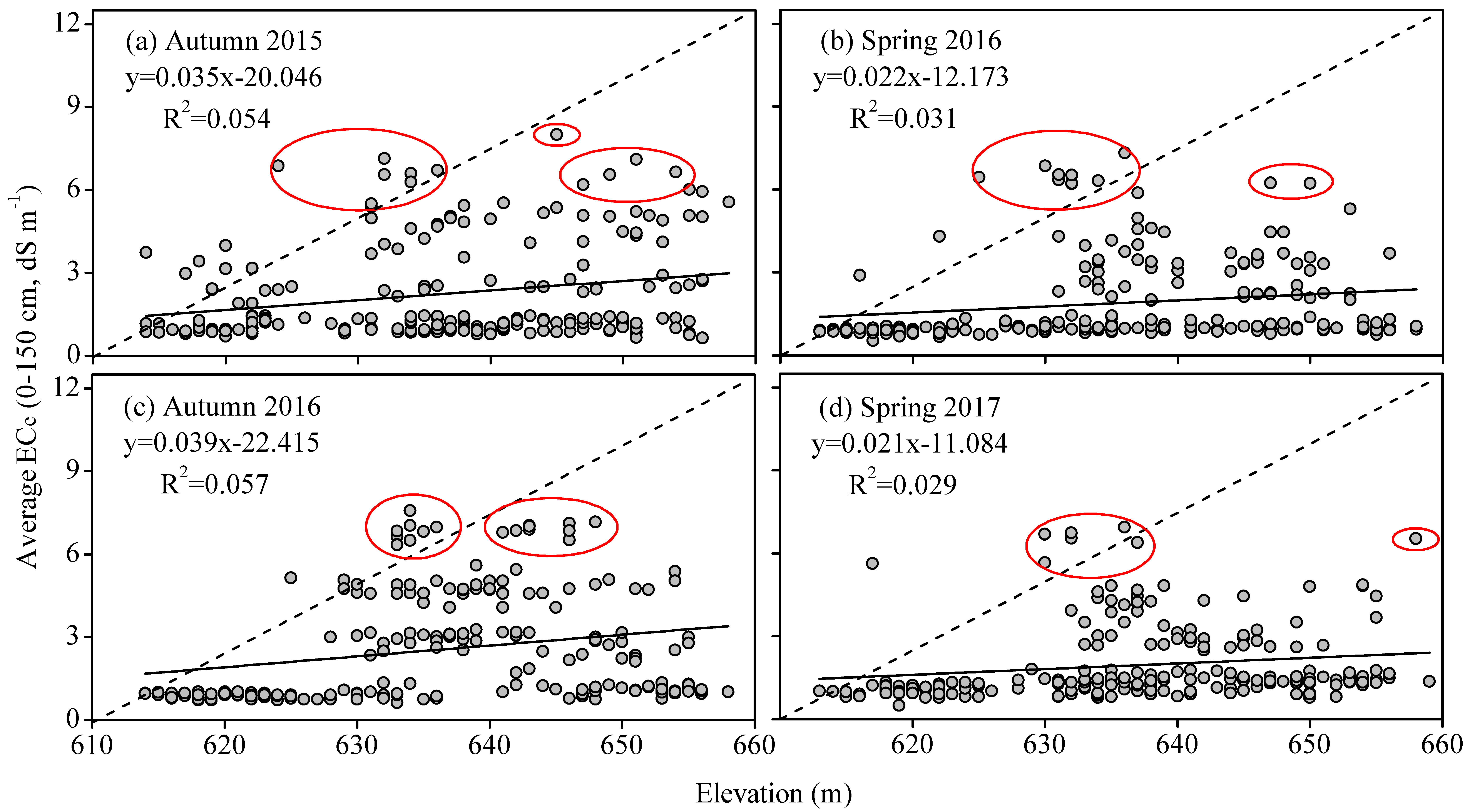
4.3. Effects of Topography on Soil Salinity

Topography affects hydrological processes (e.g., runoff and drainage) on a regional scale and affects the movements of soil water and salt, which in turn affects the spatial and temporal distribution of soil salinity [38]. To study the effect of topography on salt migration, an elevation map of the study area was obtained via digital elevation model (DEM) extraction (Figure 1). The terrain in the South is higher than in the North, and the difference was as much as 60 m. Figure 9 presented a series of regression analyses between the elevation and the average EC_e values for the 0–150 cm soil depth of the 210 noncontiguous sample points in autumn 2015, spring 2016, autumn 2016, and spring 2017. The values of R² were 0.054, 0.031, 0.057, and 0.029, respectively, and no significant correlations were observed between the elevation and the average EC_e values for the 0–150 cm soil depth at a regional scale. However, there were significant correlations in some areas (Figure 9, red circles, >6 dS m⁻¹), the changes of microtopography may affected the spatial variation of soil salinity due to the uneven movements of soil water and salt. Collectively, the spatial patterns that are shown in Figure 1 and Figure 4 suggested two major landforms in the field: The swale and relatively higher-lying slope. The EC_e values were generally higher in the swales or in areas with rather poor drainage, whereas the values were lower in relatively higher-lying slopes or that were well-drained. Therefore, microtopography was the major factor influencing spatial distribution of soil salinity in the study area.

4.4. Management of Soil Water and Salt

The distribution of soil salinity is highly heterogeneous due to the migration of salt in fields, which has always been concerned by researchers and growers in arid and semiarid areas. Therefore, proper management of soil water and salt is important for improving the yields of crop, as well as the sustainable development of agriculture. This includes optimal irrigation management (e.g., timing and amounts) and improving the regional hydraulic engineering infrastructure (e.g., irrigation and drainage canal) [39]. In order to obtain the distribution of soil salinization, monitoring systems are required to provide both negative and positive feedback. In the non-saline or slightly saline soil areas, the management should be focused on preventing the increase of salt content due to unreasonable human activities. In the moderately or strongly saline areas, the irrigation and drainage processes should be managed carefully to avoid further deterioration of soil and water quality. Specifically, within the suggested range of seasonal irrigation amount, properly increasing the frequency of irrigation would reduce unnecessary consumption of evaporation and leaching and keep the yields of crop. For some high salinity zoning, there could be carried out some desalting activities to ensure the growth of crop. In addition, there need to reduce natural evapotranspiration before the periods of harvest and planting, and make full use of irrigation water in autumn and snowmelt water in spring. Drainage of salt from within, and near, the fields should be carried out using canals during these periods to reduce the influence of soil salinity on the future growth of crop.

5. Conclusions

The migration processes of soil water and salt are complicated in irrigated agricultural areas due to differences in seasonal water application patterns, strong evaporation, topography, and human activities. In this study, we attempt to investigate the 3-D spatial variation and influencing factors of seasonal soil salinity in cold and semiarid irrigated rice fields using 3-D scatter data model and 3-D mesh model. The study shows that hydrological processes and microtopography were the main factors affecting the spatiotemporal variation and migration of soil salinity, which resulted in different spatial distribution patterns of soil salinity in different seasons. The horizontal migration of soil salinity was small with a dispersion trend from autumn to spring due to the limitation of snowmelt water; migration was great with an accumulation trend from spring to autumn due to an abundance of irrigation water. Vertically, soil soluble salt accumulated in the soil surface due to high evaporation and accumulated in the deeper subsoil due to leaching and drainage. The results showed that the average EC_e values in vertical profiles decreased from autumn to spring, and increased from spring to autumn. In addition, microtopography was the major factor influencing spatial distribution and migration of soil salinity in different seasons. Soil salinity was generally accumulated in the swales or in areas with rather poor drainage, whereas salt content was generally lower in relatively higher-lying slopes or those that were well-drained. Combining the kriging interpolation method based on 3-D scatter data model and 3-D mesh model, we can obtain the seasonal 3-D spatial distribution of soil salinity efficiently. The results will provide basic knowledge and practical values for 3D Gis-mapping and sustainable management of seasonal soil water and salt in irrigated agricultural areas and other similar areas.

References

1. Scudiero, E.; Skaggs, T.H.; Corwin, D.L. Comparative regional–scale soil salinity assessment with near–ground apparent electrical conductivity and remote sensing canopy reflectance. Ecol. Indic. 2016, 70, 276–284. [Google Scholar] [CrossRef] [Green Version]
2. Xing, X.; Du, W.; Ma, X. Field–scale distribution and heterogeneity of soil salinity in the mulched–drip–irrigation cotton field. Arch. Agron. Soil Sci. 2019, 65, 1248–1261. [Google Scholar] [CrossRef]
3. Bailey, R.T.; Tavakoli–Kivi, S.; Wei, X. A salinity module for SWAT to simulate salt ion fate and transport at the watershed scale. Hydrol. Earth Syst. Sc. 2019, 23, 3155–3174. [Google Scholar] [CrossRef] [Green Version]
4. Connor, J.D.; Schwabe, K.; King, D.; Knapp, K. Irrigated agriculture and climate change: The influence of water supply variability and salinity on adaptation. Ecol. Econ. 2012, 77, 149–157. [Google Scholar] [CrossRef]
5. Metternicht, G.I.; Zinck, J.A. Remote sensing of soil salinity: Potentials and constraints. Remote Sens. Environ. 2003, 85, 1–20. [Google Scholar] [CrossRef]
6. Shao, H.; Chu, L.; Lu, H.; Qi, W.; Chen, X.; Liu, J.; Kuang, S.; Tang, B.; Won, V. Towards sustainable agriculture for the salt–affected soil. Land Degrad. Dev. 2019, 30, 574–579. [Google Scholar] [CrossRef]
7. Bless, A.E.; Colin, F.; Crabit, A.; Devaux, N.; Philippon, O.; Follain, S. Landscape evolution and agricultural land salinization in coastal area: A conceptual model. Sci. Total Environ. 2018, 625, 647–656. [Google Scholar] [CrossRef]
8. Shouse, P.J.; Goldberg, S.; Skaggs, T.H.; Soppe, R.W.O.; Ayars, J.E. Changes in spatial and temporal variability of SAR affected by shallow groundwater management of an irrigated field, California. Agr. Water Manag. 2010, 97, 673–680. [Google Scholar] [CrossRef]
9. Li, X.; Chang, S.X.; Salifu, K.F. Soil texture and layering effects on water and salt dynamics in the presence of a water table: A review. Environ. Rev. 2014, 22, 41–50. [Google Scholar] [CrossRef]
10. Xu, L.; Zheng, C.L.; Wang, Z.C.; Nyongesah, M.J. A digital camera as an alternative tool for estimating soil salinity and soil surface roughness. Geoderma 2019, 341, 68–75. [Google Scholar] [CrossRef]
11. Bazihizina, N.; Barrett–Lennard, E.G.; Colmer, T.D. Plant growth and physiology under heterogeneous salinity. Plant Soil 2012, 354, 1–19. [Google Scholar] [CrossRef]
12. Corwin, D.L.; Lesch, S.M. A simplified regional–scale electromagnetic induction – Salinity calibration model using ANOCOVA modeling techniques. Geoderma 2014, 230, 288–295. [Google Scholar] [CrossRef]
13. Liu, W.; Lu, F.; Xu, X.; Chen, G.; Fu, T.; Su, Q. Spatial and temporal variation of soil salinity during dry and wet seasons in the southern coastal area of Laizhou Bay, China. Indian J. Geo–Mar. Sci. 2020, 49, 260–270. [Google Scholar]
14. Nouri, H.; Borujeni, S.C.; Alaghmand, S.; Anderson, S.J.; Sutton, P.C.; Parvazian, S.; Beecham, S. Soil salinity mapping of urban greenery using remote sensing and proximal sensing techniques; the case of Veale Gardens within the Adelaide Parklands. Sustainability 2018, 10, 2826. [Google Scholar] [CrossRef] [Green Version]
15. Wang, Y.; Deng, C.; Liu, Y.; Niu, Z.; Li, Y. Identifying change in spatial accumulation of soil salinity in an inland river watershed, China. Sci. Total Environ. 2018, 621, 177–185. [Google Scholar] [CrossRef]
16. Liu, F.; Zhang, G.-L.; Song, X.; Li, D.; Zhao, Y.; Yang, J.; Wu, H.; Yang, F. High–resolution and three–dimensional mapping of soil texture of China. Geoderma 2020, 361, 114061. [Google Scholar] [CrossRef]
17. Liu, W.; Xu, X.; Lu, F.; Cao, J.; Li, P.; Fu, T.; Chen, G.; Su, Q. Three–dimensional mapping of soil salinity in the southern coastal area of Laizhou Bay, China. Land Degrad. Dev. 2018, 29, 3772–3782. [Google Scholar] [CrossRef]
18. Zare, E.; Beucher, A.; Huang, J.; Boman, A.; Mattback, S.; Greve, M.H.; Triantafilis, J. Three–dimensional imaging of active acid sulfate soil using a DUALEM–21S and EM inversion software. J Environ. Manag. 2018, 212, 99–107. [Google Scholar] [CrossRef]
19. Zhang, S.; Zhang, L.; Li, Z.; Wang, Q.; Cui, H.; Sun, Z.; Ge, C.; Liu, H.; Huang, Y. Three–dimensional stochastic simulations of soil clay and its response to sampling density. Comput. Electron. Agr. 2017, 142, 273–282. [Google Scholar]
20. Jiang, Q.; Peng, J.; Biswas, A.; Hu, J.; Zhao, R.; He, K.; Shi, Z. Characterising dryland salinity in three dimensions. Sci. Total Environ. 2019, 682, 190–199. [Google Scholar] [CrossRef]
21. Van Meirvenne, M.; Maes, K.; Hofman, G. Three–dimensional variability of soil nitrate–nitrogen in an agricultural field. Biol. Fert. Soils 2003, 37, 147–153. [Google Scholar] [CrossRef]
22. Triantafilis, J.; Laslett, G.M.; McBratney, A.B. Calibrating an electromagnetic induction instrument to measure salinity in soil under irrigated cotton. Soil Sci. Soc. Am. J. 2000, 64, 1009–1017. [Google Scholar] [CrossRef]
23. Rhoades, J. Salinity: Electrical conductivity and total dissolved solids. In Methods of Soil Analysis: Part 3—Chemical Methods; Sparks, D.L., Ed.; Book Series No., 5; Soil Science Society of America: Madison, WI, USA, 1996; pp. 417–435. [Google Scholar]
24. Goovaerts, P. Geostatistics in soil science: State–of–the–art and perspectives. Geoderma 1999, 89, 1–45. [Google Scholar] [CrossRef]
25. Liebhold, A.M.; Rossi, R.E.; Kemp, W.P. Geostatistics and geographic information systems in applied insect ecology. Annu. Rev. Entomol. 1993, 38, 303–327. [Google Scholar] [CrossRef]
26. Chen, C.; Hu, K.; Li, W.; Li, Z.; Li, B. Three–dimensional mapping of clay content in alluvial soils using hygroscopic water content. Environ. Earth Sci. 2015, 73, 4339–4346. [Google Scholar] [CrossRef]
27. Liu, G.; Li, J.; Zhang, X.; Wang, X.; Lv, Z.; Yang, J.; Shao, H.; Yu, S. GIS–mapping spatial distribution of soil salinity for Eco–restoring the Yellow River Delta in combination with Electromagnetic Induction. Ecol. Eng. 2016, 94, 306–314. [Google Scholar] [CrossRef]
28. Cambardella, C.A.; Moorman, T.B.; Novak, J.M.; Parkin, T.B.; Karlen, D.L.; Turco, R.F.; Konopka, A.E. Field–scale variability of soil properties in central Iowa soils. Soil Sci. Soc. Am. J. 1994, 58, 1501–1511. [Google Scholar] [CrossRef]
29. Chien, Y.J.; Lee, D.Y.; Guo, H.Y.; Houng, K.H. Geostatistical analysis of soil properties of mid–west Taiwan soils. Soil Sci. 1997, 162, 291–298. [Google Scholar] [CrossRef]
30. Li, H.Y.; Shi, Z.; Webster, R.; Triantafilis, J. Mapping the three–dimensional variation of soil salinity in a rice–paddy soil. Geoderma 2013, 195, 31–41. [Google Scholar] [CrossRef]
31. Rengasamy, P. World salinization with emphasis on Australia. J. Exp. Bot. 2006, 57, 1017–1023. [Google Scholar] [CrossRef] [Green Version]
32. Bargaz, A.; Nassar, R.M.A.; Rady, M.M.; Gaballah, M.S.; Thompson, S.M.; Brestic, M.; Schmidhalter, U.; Abdelhamid, M.T. Improved salinity tolerance by phosphorus fertilizer in two phaseolus vulgaris recombinant inbred lines contrasting in their P–efficiency. J. Agron. Crop Sci. 2016, 202, 497–507. [Google Scholar] [CrossRef]
33. Yimit, H.; Eziz, M.; Mamat, M.; Tohti, G. Variations in groundwater levels and salinity in the Ili River Irrigation Area, Xinjiang, northwest China: A geostatistical approach. Int. J. Sust. Dev. World 2011, 18, 55–64. [Google Scholar] [CrossRef]
34. Sidike, A.; Zhao, S.; Wen, Y. Estimating soil salinity in Pingluo County of China using QuickBird data and soil reflectance spectra. Int. J. Appl. Earth Obs. 2014, 26, 156–175. [Google Scholar] [CrossRef]
35. Wang, Y.; Li, Y.; Xiao, D. Catchment scale spatial variability of soil salt content in agricultural oasis, Northwest China. Environ. Earth Sci. 2008, 56, 439–446. [Google Scholar] [CrossRef]
36. Gebremeskel, G.; Gebremicael, T.; Kifle, M.; Meresa, E.; Gebremedhin, T.; Girmay, A. Salinization pattern and its spatial distribution in the irrigated agriculture of Northern Ethiopia: An integrated approach of quantitative and spatial analysis. Agr. Water Manag. 2018, 206, 147–157. [Google Scholar] [CrossRef]
37. Wu, C.; Liu, Q.; Ma, G.; Liu, G.; Yu, F.; Huang, C.; Zhao, Z.; Liang, L. A study of the spatial difference of the soil quality of the Mun River Basin during the rainy season. Sustainability 2019, 11, 3423. [Google Scholar] [CrossRef] [Green Version]
38. Dessalegn, D.; Beyene, S.; Ram, N.; Walley, F.; Gala, T.S. Effects of topography and land use on soil characteristics along the toposequence of Ele watershed in southern Ethiopia. Catena 2014, 115, 47–54. [Google Scholar] [CrossRef]
39. Feike, T.; Khor, L.Y.; Mamitimin, Y.; Ha, N.; Li, L.; Abdusalih, N.; Xiao, H.; Doluschitz, R. Determinants of cotton farmers’ irrigation water management in arid Northwestern China. Agr. Water Manag. 2017, 187, 1–10. [Google Scholar] [CrossRef]
Figure 1. Location and elevation of the study area (Base on map sources: GS (2010) 1540). Source: Author.
Sustainability 12 06645 g001
Figure 2. The process of three-dimensional (3-D) GIS-mapping: (a) 3-D scatter data map, (b) 3-D mesh model map, and (c) 3-D distribution map. Source: Author.
Sustainability 12 06645 g002
Figure 3. The distribution of 3-D scatter data of soil ECe in (a) autumn 2015, (b) spring 2016, (c) autumn 2016, and (d) spring 2017. Source: Author.
Sustainability 12 06645 g003
Figure 4. 3-D spatial distribution maps of soil ECe in autumn 2015 (a), spring 2016 (b), autumn 2016, (c), and spring 2017 (d). Source: Author.
Sustainability 12 06645 g004
Figure 5. The area statistics (%) of different soil salinity levels in autumn 2015 (a), spring 2016 (b), autumn 2016 (c), and spring 2017 (d). Source: Author.
Sustainability 12 06645 g005
Figure 6. Typical cross–sections of the 3-D soil profiles in autumn 2015 (a), spring 2016 (b), autumn 2016 (c), and spring 2017 (d). Source: Author.
Sustainability 12 06645 g006
Figure 7. Box plots of soil ECe in autumn 2015 (a), spring 2016 (b), autumn 2016 (c), and spring 2017 (d). The horizontal full line in each box signifies the median value, the average values are circles, and the bottoms and tops of the boxes represent the 25th and 75th percentiles, respectively. The whiskers display the minimum and maximum values, and the black triangle indicates the outliers. Source: Author.
Sustainability 12 06645 g007
Figure 8. Changes in the average soil water content at the depths of 5, 30, 60, 90, 120, and 150 cm: (a) Monthly average water content, (b) daily water content in spring, and (c) daily water content in autumn. Source: Author.
Sustainability 12 06645 g008
Figure 9. Regional elevation versus the average ECe values for the 0–150 cm soil depth in autumn 2015 (a), spring 2016 (b), autumn 2016 (c), and spring 2017 (d). The dashed line represents the diagonal line, and the solid line represents the fitting line (n = 210). Source: Author.
Sustainability 12 06645 g009