Development of Driving Cycle Construction for Hybrid Electric Bus: A Case Study in Zhengzhou, China


School of Transportation, Southeast University, Nanjing 211189, China
*
Author to whom correspondence should be addressed.
Sustainability 2020, 12(17), 7188; https://0-doi-org.brum.beds.ac.uk/10.3390/su12177188
Submission received: 30 July 2020
/
Revised: 25 August 2020
/
Accepted: 27 August 2020
/
Published: 3 September 2020
(This article belongs to the Collection Emerging Technologies and Sustainable Road Safety)
Abstract
:A driving cycle is important to accomplish an accurate depiction of a vehicle’s driving characteristics as the traction motor’s flexible response to stop and start commands. In this paper, the driving cycle construction of an urban hybrid electric bus (HEB) in Zhengzhou, China is developed in which a measurement system integrating global positioning and inertial navigation function is used to acquire driving data. The collected data are then divided into acceleration, deceleration, uniform, and stop fragments. Meanwhile, the velocity fragments are classified into seven state clusters according to their average velocities. A transfer matrix applied to reveal the transfer relationship of velocity clusters can be obtained with statistical analysis. In the third stage, a three-part construction method of driving cycle is designed. Firstly, according to the theory of Markov chain, all the alternative parts that satisfy the construction’s precondition are selected based on the transfer matrix and Monte Carlo method. The Zhengzhou urban driving cycle (ZZUDC) could be determined by comparing the performance measure (PM) values subsequently. Eventually, the method and the cycle are validated by the high correlation coefficient (0.9972) with original data of ZZUDC than that of the other driving cycle (0.9746) constructed with traditional micro-trip and as well by comparing several statistical characteristics of ZZUDC and seven international cycles. Particularly, with around 20.5 L/100 km fuel and approximately 12.8 kwh/100 km electricity consumption, there is a narrow gap between the energy consumption of ZZUDC and WVUCITY, and their characteristics are similar.
1. Introduction
Recently, hybrid electric buses (HEB) with better energy consumption and environmental protection performance compared with traditional fuel engine buses have been adopted in many Chinese cities and become a hot research topic [1].
As an evaluation standard and a detection criterion of vehicle emissions and fuel consumption, driving cycle is an important design basis for vehicle power matching and fuel economy optimization [2,3]. Driving cycle is a velocity–time trace that describes driving characteristics of specific vehicles in specific traffic environments (such as urban road or expressway). Usually, it is a representative running condition which is extracted from a large amount of measured driving data using mathematical and statistical methods. Different regions have different driving characteristics; hence, developing a typical driving cycle for each place according to its situation is essential [4]. The current dominant methods of driving cycle construction include the micro-trip method, fixed step analysis method, velocity–acceleration analysis method, wavelet analysis method, and Markov analysis method [5,6,7,8]. Many scholars have investigated the development of urban driving cycles based on the aforementioned approaches. For example, the driving cycle for electric vehicles in the city of Florence was established, combined with the collected data, micro-trip division, characteristic parameter calculation, and driving sequences clustering [9]. A multi-scale fixed step future driving cycle prediction method is presented based on adaptative online prediction [10]. Wavelet analysis was implemented in a case study of Changchun City to decompose driving cycle information into signals and take careful observations of them [11]. Besides the above, in recent years, Markov chain was applied by many researchers to design driving cycles due to its significant theoretical advantages compared with the traditional method with respect to using vehicle acceleration to divide velocity fragments to remarkably reflect the variation law of velocity in the original data. Lin Jie firstly proposed a Markov analysis method in the study of conventional vehicle driving cycle analysis [12]. The Markov process is a stochastic process with no after-effect, which means that, during the random process of the known current state’s alteration, the future value only depends on the current state and is unrelated to previous ones [5]. This physical process can exactly reflect the changing trend of velocity with driving time. In the process of fragment selection, the Markov analysis method replaces the traditional random selection with transfer matrix estimation, which substantially improves the construction accuracy of driving cycles [13,14]. Liu et al. used the Markov process to design time-variant driving cycles [15]. To improve the efficiency in simulation, a three-parameter driving cycle generation method based on Markov chain was also proposed [16]. However, the majority of the current construction methods of driving cycle are primarily aimed at conventional vehicles [17,18,19,20,21]; hybrid electric vehicles (HEV) are quite different from these vehicles in the driving process due to their special powertrain structure and energy consumption modes [22,23]. Additionally, the driving cycle for HEB is more fixed compared with private HEVs. If we directly use the conventional vehicle driving data-based driving cycle to design the energy management strategy of HEB, the actual emissions and fuel consumption would not be reliable. Moreover, most of the current methods fail to consider road slope as a characteristic parameter, which would significantly affect the dynamic performance and energy consumption of HEBs since they are heavier compared with traditional HEVs. As a result, designs ignoring road slope can violate the design requirements of the longitudinal gradient in the urban road design code and become unrealistic.
Hence, motivated by the above observations, this paper proposes a driving cycle construction method for HEB based on the Markov chain theory via a case study in Zhengzhou, China. The main contribution includes the following: (1) a complete Markov analysis-based urban driving cycle construction process is formulated, considering not only velocity but also road slope; (2) velocity state cluster division principle and the performance evaluation criteria of driving cycle are designed; (3) a special performance measure calculation method for driving cycle candidate duration selection is proposed, which improved the traditional method by incorporating normalization.
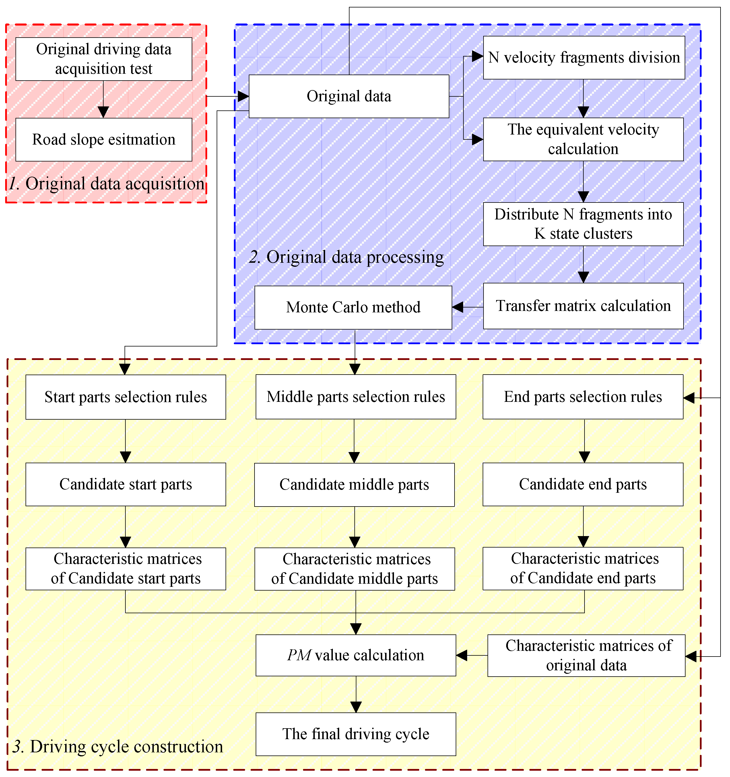
The construction process of the proposed driving cycle is shown in Figure 1. Section 2 describes the acquisition of original HEB driving data acquisition. The original data processing is given in Section 3 while Section 4 illustrates the driving cycle construction of each part. Section 5 validates the proposed ZZUDC (Zhengzhou urban driving cycle) by comparing with the traditional micro-trip method and other international cycles. Finally, Section 6 concludes this paper.
2. The HEB Original Driving Data Acquisition
The HEB original driving data can reflect the urban traffic conditions and HEB driving characteristics, which is the source of data for driving cycle construction. The more details of the original driving data used in the construction process, the more objective and representative the driving cycle’s characteristics would be. Two representative HEB lines of Zhengzhou City in China are selected as the experimental objects of the driving data acquisition test after thorough consideration based on the test route, choosing rule proposed below. Note that we assume that HEB can work in pure electric driving mode at low velocity.
2.1. The Selection of Test Route and Test HEB
2.1.1. Test Route Selection
The rules for choosing the test route are as follows:
- Hybrid electric bus is the only choice to drive on the test route.
- The test route should include both traditional and rapid bus routes.Bus rapid transit (BRT) is a new type of public transport system running between the railway and traditional bus transportation. BRT uses the special bus route to achieve rail transit mode operation, and it has been applied widely in China. The driving states of buses in the BRT routes are totally different from those in the traditional bus routes. Therefore, the construction of an urban driving cycle which fuses traditional bus route and rapid bus route is consistent with the actual operation situation of Chinese urban buses.
- The selected bus route should cover congested and fluent urban regions.
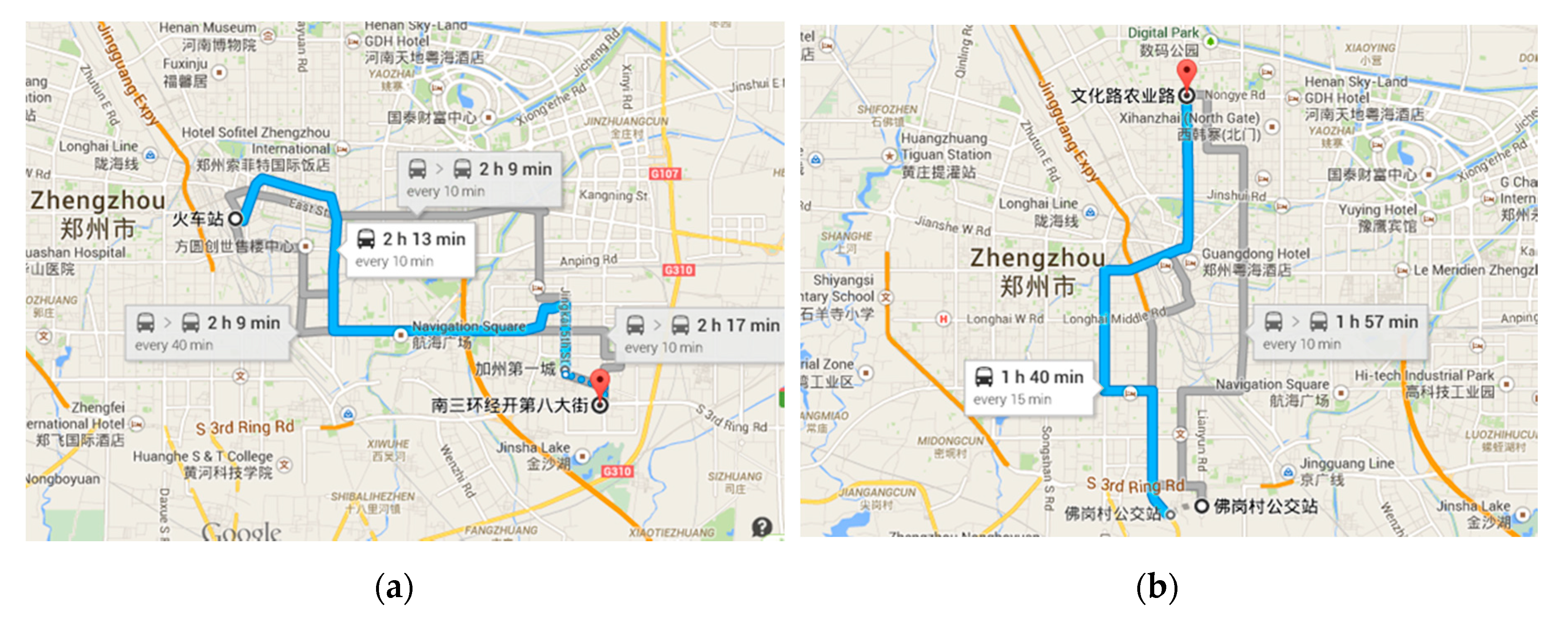
According to the above three rules, the BRT route B17 and traditional bus route 906 are selected as the test routes, which are shown in Figure 2 and Table 1.
As can be seen in Figure 2, BRT route B17 runs from east to west, passing through crowded areas including railway stations and commercial centers, as well as residential areas, factories, schools, parks, and urban landmark scenic spots. Meanwhile, bus route 906 runs from south to north, passing through bus stations, universities, government offices, and other important urban facilities. The two lines cover all levels of roads in the urban area of Zhengzhou and account for roughly the same proportion for all levels of roads.
2.1.2. Test Bus Selection
The HEB that drives on bus route 906 is the same as that on BRT route B17. Thus, there is no difference between buses in the process of the fusing of the aforementioned two bus routes for urban driving cycle construction. The specific parameters of the test HEB are shown in Table 2.
2.2. The Driving Data Acquisition System
A global positioning and inertial navigation system (GPS/INS integrated system) named OXTS inertial+ is used for the HEB driving data acquisition. The measurement parameters include velocity, transient acceleration, and road slope. The location precision of measurement is 2 cm 1σ, and velocity precision is 0.05 km/hRMS. As for the acceleration precision, the error is 10 mm/s2 1σ, linearity is 0.01%, and the total range is 100 m/s2.
2.2.1. Velocity and Acceleration Measurement
Compared with the traditional method, in which the driving data are read by the anti-lock braking system (ABS) speed signal, the GPS receiver can not only measure bus velocity with higher precision but also acquire the bus altitude and location for road slope estimation. The bus acceleration information is measured by the inertial navigation system, and the measurement error will not increase with the enhancement of sampling frequency. In order to retain more details of velocity fragments, the test sampling frequency is set to 5 Hz.
2.2.2. Road Slope Estimation
As indicated, other than velocity, road slope is also a particularly important characteristic for HEBs in control and design. This paper estimates road slope by calculating the ratio for the altitude difference between two sampling times to the horizontal distance traveled by the HEB during the sampling period and then taking the arctangent, which follows the equation
where is the altitude change between the previous and current sampling time, is the bus horizontal velocity, is the sampling period.
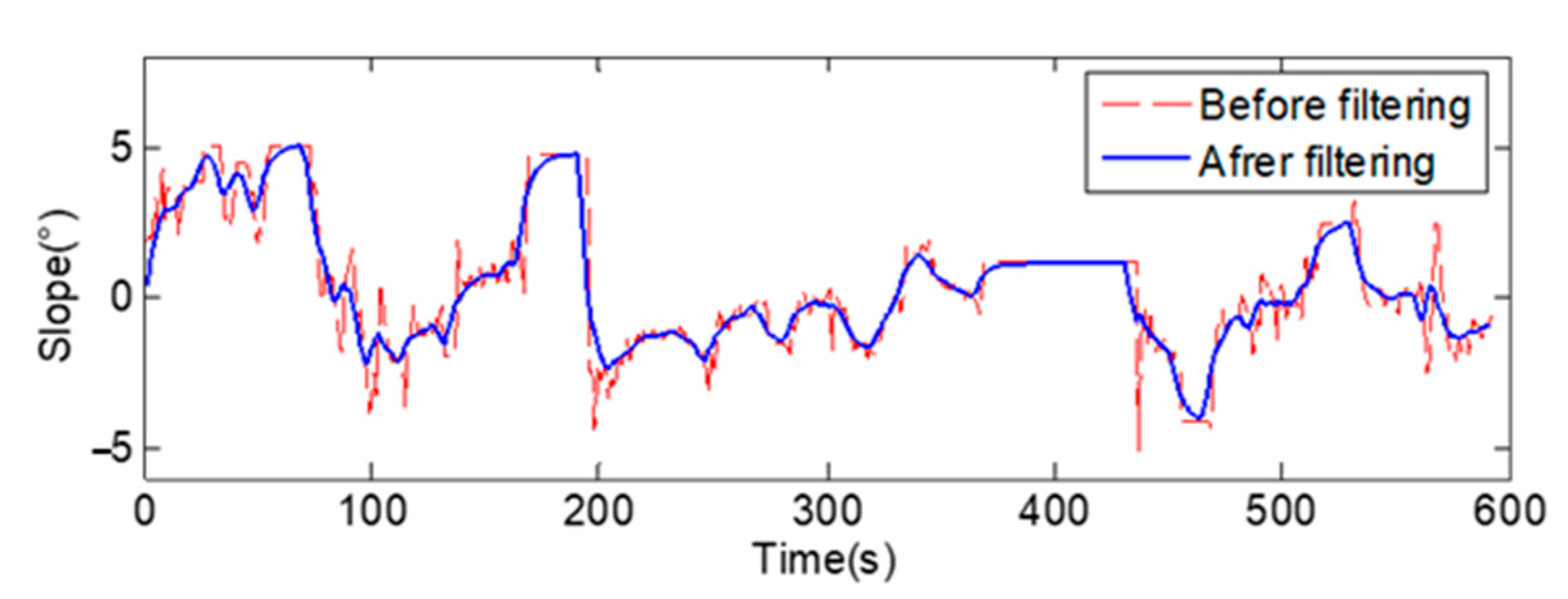
The road slope can be calculated with Equation (1); however, the computed preliminary results have high magnitude and some of the points obviously violate the longitude slope design requirements of the China code for design of urban road engineering [24]. Hence, the road slope preliminary values need to be filtered, the steps of which are as follows:
- Primarily, eliminate slope calculated values with low velocity to avoid the denominator of Equation (1) being close to 0.
- Carry out filtering. If the calculated slope values are higher than 9% [25], then replace them with those of the previous sampling time.
- Perform average filtering against the processed slope values to smooth out the sawtooth signals.
The road slope after filtering is partially shown in Figure 3.
3. Original Data Preprocessing
The original data preprocessing consists of four steps: velocity fragment division, fragment state cluster distribution analysis, the Markov transfer matrix calculation, and characteristic parameter analysis. Among these four steps, the transfer matrix calculation is the most essential step of data preprocessing and driving cycle construction. The velocity fragment division and its state cluster distribution analysis have a direct influence on the accuracy of the Markov transfer matrix, and analysis of characteristic parameters is a criterion used to judge whether the characteristics of the constructed driving cycle agree with that of the original driving data.
3.1. Velocity Fragment Division
A velocity fragment is the minimum unit of the driving cycle construction, which is abstracted from the original data according to specific rules.
3.1.1. Velocity Threshold Determination
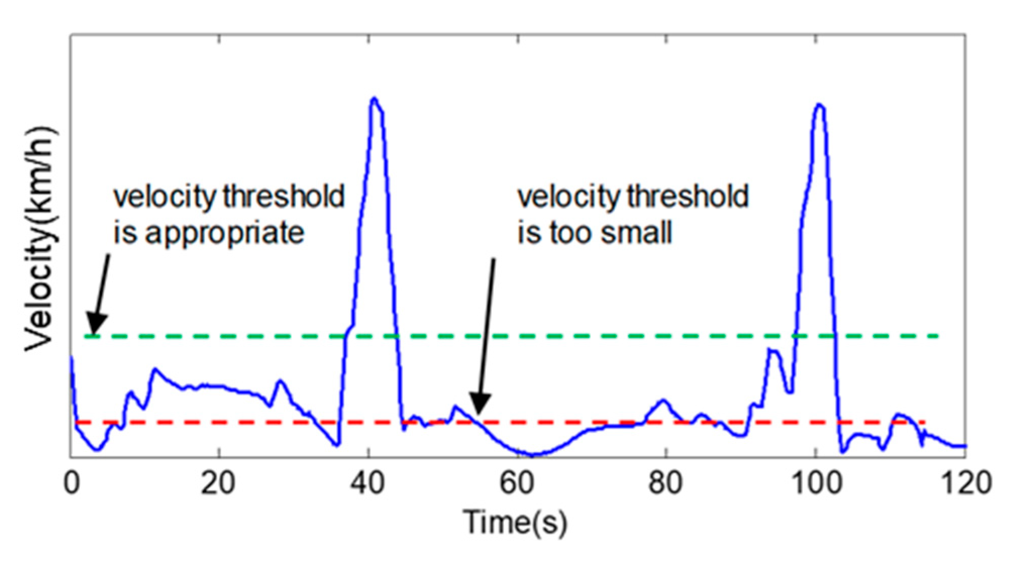
The HEB generally drives in pure electric mode at a low velocity without an idling state. Therefore, it is necessary to consider the distinction between the shutdown state and driving state at a low velocity. The HEB operates in a shutdown state when the current velocity is smaller than a threshold value. However, when the velocity threshold is set to be extremely small, as shown in Figure 4, the fluctuant velocity in a small range will be cut into a great many shutdown fragments, which does not match the actual situation and will affect the analysis of characteristic parameters.
Based on the above consideration, the velocity sampling points below 4 km/h are separated from the original data and the distribution of different velocity intervals is analyzed. The corresponding statistical data are shown in Table 3.
It can be seen that the sampling points below 0.7 km/h can represent 67.33% of the population. Meanwhile, the velocity threshold value should be constricted as an appropriately small value. Thus, 0.7 km/h is selected as the velocity threshold of stop fragments after comprehensive consideration.
3.1.2. Acceleration Threshold Determination
The HEB is considered to travel at a uniform velocity when the bus’s acceleration fluctuates within the threshold range. As in the previous discussion, when the velocity is below 0.7 km/h, the sampling points will be divided into shutdown fragments, and the acceleration of these sampling points should also theoretically fluctuate within a small range. The absolute values of acceleration distribution of shutdown fragments are analyzed, and the statistical data are shown in Table 4.
As shown in Table 4, around 92.01% of acceleration sampling points are in the interval of (0, 0.1 m/s2), which indicates that the HEB drives at a uniform velocity when the acceleration is in the interval of (−0.1, 0.1). Considering that the road bump may magnify the measurement error of acceleration, the selection value of final acceleration threshold can approximately rise to 0.15 m/s2.
3.1.3. Basis of Velocity Fragment Division
In general, the values of both sampling velocity and acceleration should account for fragment division. The original data are divided into four types of velocity fragment: shutdown (stop) fragment, acceleration fragment, deceleration fragment, and uniform fragment. The basis of fragment division is shown in Figure 5.
3.2. Fragement State Cluster Distribution
3.2.1. Calculation of Required Power and Nominal Velocity
Every sampling time in the original driving data corresponds to the information of the velocity, acceleration, road slope, etc. To comprehensively depict the driving feature with fragment cluster distribution, the required power is also an important factor, which can be computed with Equations (2) and (3).
where P0(a > 0.15) denotes the required power of acceleration fragment when bus acceleration a > 0.15 m/s2, P0(a ≤ 0.15) represents the required power of non-acceleration fragment when a ≤ 0.15 m/s2. ua is the bus velocity, i is the road slope, G is the bus gravity, f is the rolling resistance coefficient, CD is the drag coefficient, A is the bus windward area, and ηT means the bus powertrain mechanical efficiency.
Required power is an unintuitive parameter of fragment division and state cluster distribution; meanwhile, as position information, the road slope cannot be directly added into the velocity–time trace. Therefore, the nominal velocity with the same required power and acceleration is a suitable method to involve the road slope information.
The specific operations are shown in Equations (4) and (5).
When a > 0.15 m/s2,
When a ≤ 0.15 m/s2,
where u denotes the nominal velocity.
3.2.2. State Cluster Distribution
Calculate the average nominal velocity of each fragment, then distribute all velocity fragments into 7 state clusters according to the calculated average values, which are (−∞, 5], (5, 15], (15, 25), (25, 35), (45, 55), and (55, +∞). Note that the nominal velocity cannot be directly applied to the driving cycle construction, and it only works in the fragment state cluster distribution where the road slope information is added into the traditional velocity–time trace and helps to make the state cluster distribution more reasonable.
3.3. Calculation of the Markov Transfer Matrix
The bus driving process can be regarded as a discrete Markov chain. The alteration of bus velocity can be regarded as a transfer between the current and next state clusters of velocity fragment, and the transfer process satisfies the probability distribution. Define as the Markov chain and S as state space, namely
where pij(n) denotes the one step transfer probability at moment n.
The meaning of Equation (6) is the probability of model event to transfer from time n with state i to time n + 1 with state j, and the transfer matrix which represents the fragment state migration can be constructed via the transfer probabilities with different fragment states.
When state clusters are distributed, every velocity fragment has a state number. A vehicle’s driving condition transfers from one fragment to another together with the corresponding state cluster migration. The transfer matrix is calculated by including the migration of state clusters in the original data. The elements in the transfer matrix, namely the transfer probability, can be calculated as follows:
where Nij is the time of velocity fragment transferring from state i at time t − 1 to state j at time t.
Take the first row of the transfer matrix, for example. As shown in Table 5, it indicates the moments of velocity fragment transfer from state 1 to other states, and the corresponding transfer probabilities have also been counted but are omitted due to limited space. The transfer probability of other states can be calculated in the same way, and the 7 × 7 state transfer matrix T could be constituted as follows:
3.4. The Statistical Anlysis of Original Data
3.4.1. Characteristic Parameter Matrix of Original Data
A 1 × 16 original characteristic matrix M0 is then constructed to represent the original data. The PM (performance measure) value is the differences in characteristic parameters between the driving cycle and original data, which is normalized and used to represent the differentiating degree.
3.4.2. Calculation of PM Value
The calculation of PM value consists of four steps:
- Count the characteristic parameters of driving cycle candidates n and construct the n × 16 matrix M.
- Obtain the absolute differentiating value matrix pm through each row of matrix M minus the original characteristic M0:
- Normalize pm. Normalization is necessary for totally different parameter ranges, which can be deduced aswhere pmimax is the maximum value of the matrix pm’s ith column, while pmimin is the minimum one.
- Sum the elements in the kth row in the matrix PM(k,i) to obtain the PM value of the driving cycle.
3.4.3. Sufficient Proof of the Original Data
The original data are the basis of driving cycle construction and the constructed result will be more credible, with more collected original data. The volume of original data can have a strong influence on the driving cycle’s representation. In this paper, the data acquisition experiment lasted for two weeks, and more than 600,000 sampling points were acquired, which provided sufficient data for subsequent research.
As we have constructed the driving cycle based on Markov chain theory, the credibility of the Markov transition matrix can be enhanced with a larger original database. Therefore, the original data are firstly fused day by day; then, the F norm of the differentiating matrix, which can characterize the variation in Markov transition matrixes with the increase in data amount, is calculated by evaluating the difference in the two adjacent matrixes. The computing results are shown in Figure 6.
The F norm decreases gradually, and it fluctuates around a stable value after the 4th day. This phenomenon demonstrates that the Markov transfer matrix is stable and the original driving data are sufficient.
4. Driving Cycle Construction
As indicated, due to the Markov chain, the velocity of the sampling point at the next moment is completely dependent on the velocity of the sampling point at the current moment and the transition probability corresponding to this state. However, at the beginning and end of the driving cycle, HEB’s driving condition has been determined since HEB must gradually accelerate or decelerate towards a standstill state from other driving conditions. Adopting the Markov transfer matrix to construct these two parts is not advisable. Therefore, the start, middle, and end parts of the driving cycle are constructed, respectively, and then they are spliced according to the time sequence to accomplish the final driving cycle construction.
4.1. Construction of Start Part
The construction of the start part contains 2 steps. First, select all start part candidates from the original data with proposed rules. Then, the PM value of every part is calculated. To this end, we select 16 parameters to characterize the original data, as shown in Table 6.
The time length of the start part selected in this paper is 75 s. The stop duration before the bus standing start is mainly determined by the traffic condition. In Table 6, the proportion of stop time accounts for 24.09% of the original data; accordingly, the stop time in the 75 s duration of start part is no more than 18 s. Moreover, durations of stop fragments of more than 5 s make up 54.21% of all stop fragment durations, while durations longer than 10 s make up 32.85%. The stop fragments that can be used for comparison decrease with the increase in duration, which develops in an opposite trend to that for the start part selection. Therefore, the stop duration of the stop part candidate is set to 5 s.
Generally, a long-time parking situation does not appear in the start part, so the time proportion of 4 kinds of velocity fragments, the maximum, average, and minimum velocity, will not be considered during the comparison of characteristic parameters in the PM value calculation process. Only the difference between the candidate start part and the original data, which represents the acceleration, road slope, and road power, should be considered.
Then, all the start part candidates are sorted according to the PM value; the one which has the lowest PM value will be the optimal selection.
4.2. Construction of Middle Part
The construction of the middle part is solved mainly with the Monte Carlo method. A random number is generated to combine the probability distribution of the Markov transfer matrix, and then the next velocity fragment’s state cluster can be determined.
The time length of the middle part is designed to be more than 1000 s. If the start part has been constructed, the velocity and state cluster of the end point, which is also the initial point of the middle part, can be acquired.
The specific selection rules for the middle part are shown below:
- Confirm the current state cluster and the transfer probability, which are determined according to the Markov transfer matrix T.
- Generate a random number r in the interval of (0, 1), if r meets the in-equation as follows:Then, the next state cluster of velocity fragment is q.
- Determine the velocity fragments whose velocity differences in current and next state clusters are below 0.5 km/h. The one which has the minimum velocity difference will be the next determined velocity fragment.
- The sampling points which are used in the start part construction will not be used in the middle part construction, and 10 middle part candidates are constructed for optimal selection.
Combined with the constructed start part for PM value calculation, in this section, all 16 characteristic parameters are used for calculation. We chose the middle part candidate with the lowest PM value to construct the middle part of the driving cycle.
4.3. Construction of End Part
The method of end part construction is similar to that of start part; it is noteworthy that the end part candidates should be combined with the constructed start and middle parts for the PM value calculation, and similarly, the one which has the lowest PM value will be chosen as the final end part of the driving cycle considering all 16 characteristic parameters.
The selection method of the end part is the same as that of the start part. The specific selection rules for the end part are shown below:
- The velocity of the sampling points that are 10 s prior to the checkpoint is above velocity threshold 0.7 km/h.
- The velocity sampling points which are 5 s later than the checkpoint are below the velocity threshold 0.7 km/h.
- If both the above conditions are met, set the checkpoint at the time t, then the sampling points in the time interval of (t − 114, t + 5) will be chosen as the end part candidates.
- Check all sampling points in the first 60 s of every end part candidate, determine 10 whose velocities in sampling points are closest to the terminal velocity of the constructed middle part, and then set these points as the start times of the 10 end part candidates.
4.4. Construction of Driving Cycle
The PM values of the 3 parts of the driving cycle are sorted in size, as shown in Table 7. The selection details of the 3 final parts of the driving cycle can be apparently represented with the PM values. As shown in the first column of the table, the value of candidate start parts is 913, and those of the other two are both 10. The first row of the table is the lowest PM value for every part’s optimal selection.
According to the time sequence, the start, middle, and end parts of the driving cycle, which have the lowest PM values in each group, are spliced to form a complete time–velocity curve, as shown in Figure 7, which indicates that the driving cycle of the hybrid electric bus based on Markov chain has been constructed.
The mileage of the constructed driving cycle can be acquired through the integration of the velocity in time domain. Through mapping the road slope values of corresponding sampling points, the distance–slope curve shown in Figure 8 is acquired. The figure indicates that the driving distance of one driving cycle is 5 km, and the road slope is less than 4 degrees, which meets the requirements for the designing of urban road engineering.
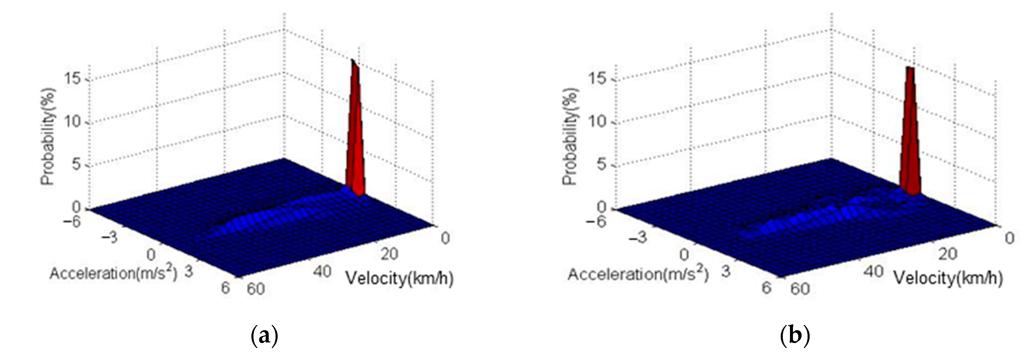
Moreover, the velocity–acceleration probability distribution (VAPD) is a decisive criterion for the representative evaluation of the constructed driving cycle [26]. The VAPDs of the original data and the constructed driving cycle are shown in Figure 9. It can be seen that the VAPD of the constructed driving cycle is similar to that of the original data, and both of them have a long stop period with relatively gentle acceleration and deceleration.
5. Validation of ZZUDC as a Driving Cycle
5.1. Comparison between the Driving Cycles Based on Markov and Traditional Micro-Trip
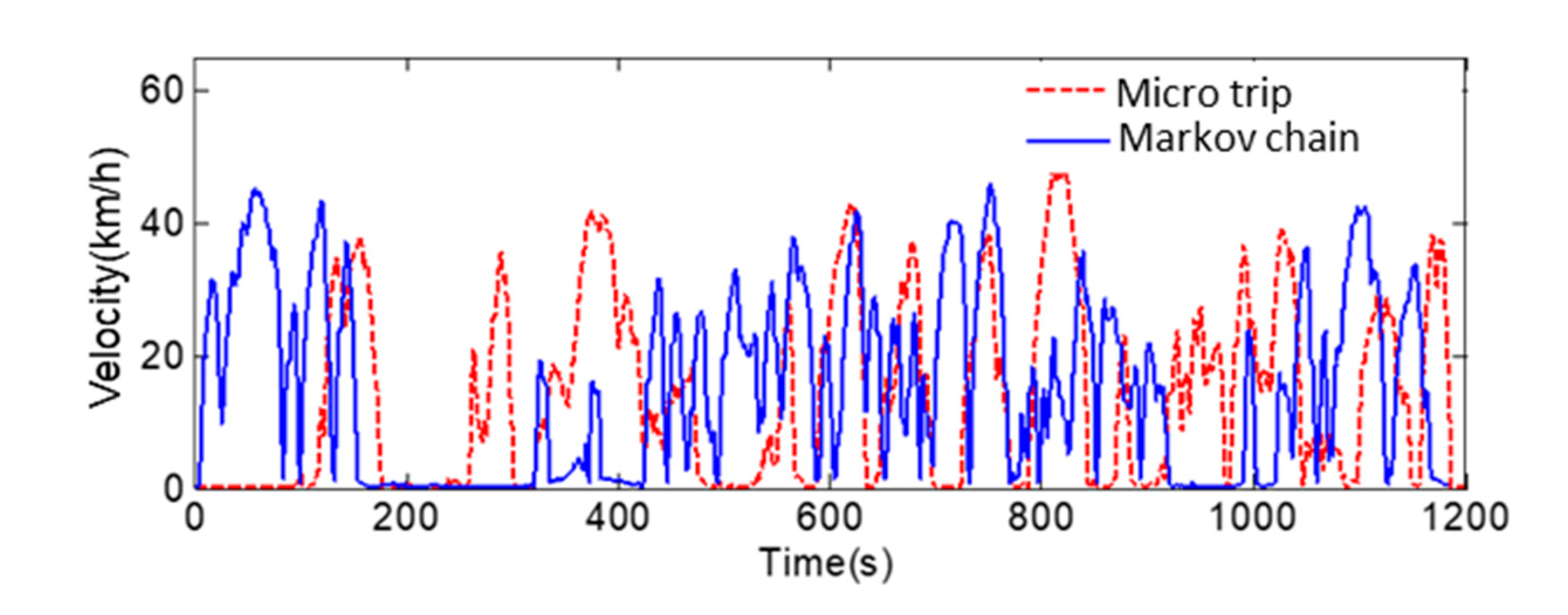
The micro-trip method is a traditional way to construct a driving cycle [27]. This paper adopts the same original date to construct a 1200 s driving cycle based on the micro-trip method. It is noteworthy that the velocity and acceleration thresholds for micro-trip separation are the same as that of the Markov chain-based method. The results of comparing the driving cycles constructed with the two methods are shown in Figure 10 and Table 8. In Table 8, most of the characteristic parameters of the driving cycle constructed with the Markov method are closer to those of the original data than the micro-trip method.
Furthermore, the similarity degree of the constructed driving cycle and the original data is represented by the correlation coefficient of characteristic parameters in this paper. The calculating equation is expressed as
where X represents the characteristic parameters of the original data, Y represents the characteristic parameters of the constructed driving cycle, Cov(X,Y) is the covariance of X and Y, and Var(X), Var(Y) are the variance of X and Y, respectively.
According to Table 8 and Equation (13), the correlation coefficient of original data and driving cycle based on the Markov chain is 0.9972, which is higher than that of the traditional micro-trip, with 0.9746. The results indicate that the Markov chain-based driving cycle is more objective and effective.
5.2. Comparison between ZZUDC and Other International Cycles
5.2.1. Dynamic Programming
The experiment vehicle is a plug-in hybrid bus [28], which weight 13,100 kg and has driven on the constructed driving cycle ZZUDC. As for the parameters of every component—for example, engine, battery, motor, etc.—these are omitted, but a related paper [28] is a decent reference.
The numbers of every driving cycle are evaluated with the same constraints. The target function of dynamic programming (DP) is
St.
where (state of charge) is a single state variable, function illustrates the time-variant model of the vehicle, and are the initial and final figures, respectively, and is the state value at kth discretized point. The control single is , including five elements which are , , , , and . The meanings of control singles are torque of engine, torque of ISG, speed of engine, state of clutch, and torque of mechanical braking, respectively. All control singles are continuous types, except for the state of clutch (), which is a 0-1 discrete type.
The constraints of this problem come from both state variables and control singles. Except for the restrictions in Equation (15), the maximum charging/discharging rate can also affect the slope of the alteration of SOC. Specific constraints of the control singles derive from the related components’ limiting speed and torque [29].
5.2.2. Comparison between the Statistical Characters of Various Driving Cycles
In order to assess the performance of ZZUDC more comprehensively, we selected seven standard international driving cycles as comparisons, which are CTUB (China typical urban bus driving cycle), LA92, IM240, JN1015 (Japan 1015), UDDS (urban dynamometer driving schedule), MANHATTAN, and WVUCITY. As can be seen in Table 9, most of the selected international driving cycles are urban route types. The total cycle durations significantly vary between cycles, ranging from 241 s (IM240) to 1408 s (WVUCITY), and mainly distribute between 1000 s and 1500 s. The duration of ZZUDC is 1184 s, which is an average level. The major difference is the highest velocity, which ranges from around 40 km/h to above 108.15 km/h. This is because different cities can have different traffic conditions, and the driving cycles should reflect the distinctions. In addition, some of the driving cycles, such as LA92, are composite driving cycles and contain both urban route types and suburban route types. The suburban part would certainly amplify the parameter of highest velocity.
However, values of some assessment parameters of the MANHATTAN and WVUCITY are close to the constructed driving cycle ZZUDC, including duration, mileage, average velocity, maximum velocity, average acceleration, and deceleration. The traveling distances of WVUCITY and ZZUDC are both around 5 km, and the gaps of average acceleration and deceleration between these two cycles are within 10%. The maximum acceleration, maximum deceleration, and analogous root mean square of acceleration (RMS of acc) of ZZUDC are similar to those of the MANHATTAN driving cycle. Moreover, the energy consumption of these two cycles is at the same level, with around 21.3 L/100 km for fuel consumption and approximately 13.3 kwh/100 km for electricity consumption for MANHATTAN and around 20.5 L/100 km fuel consumption and approximately 12.8 kwh/100 km electricity consumption for ZZUDC.
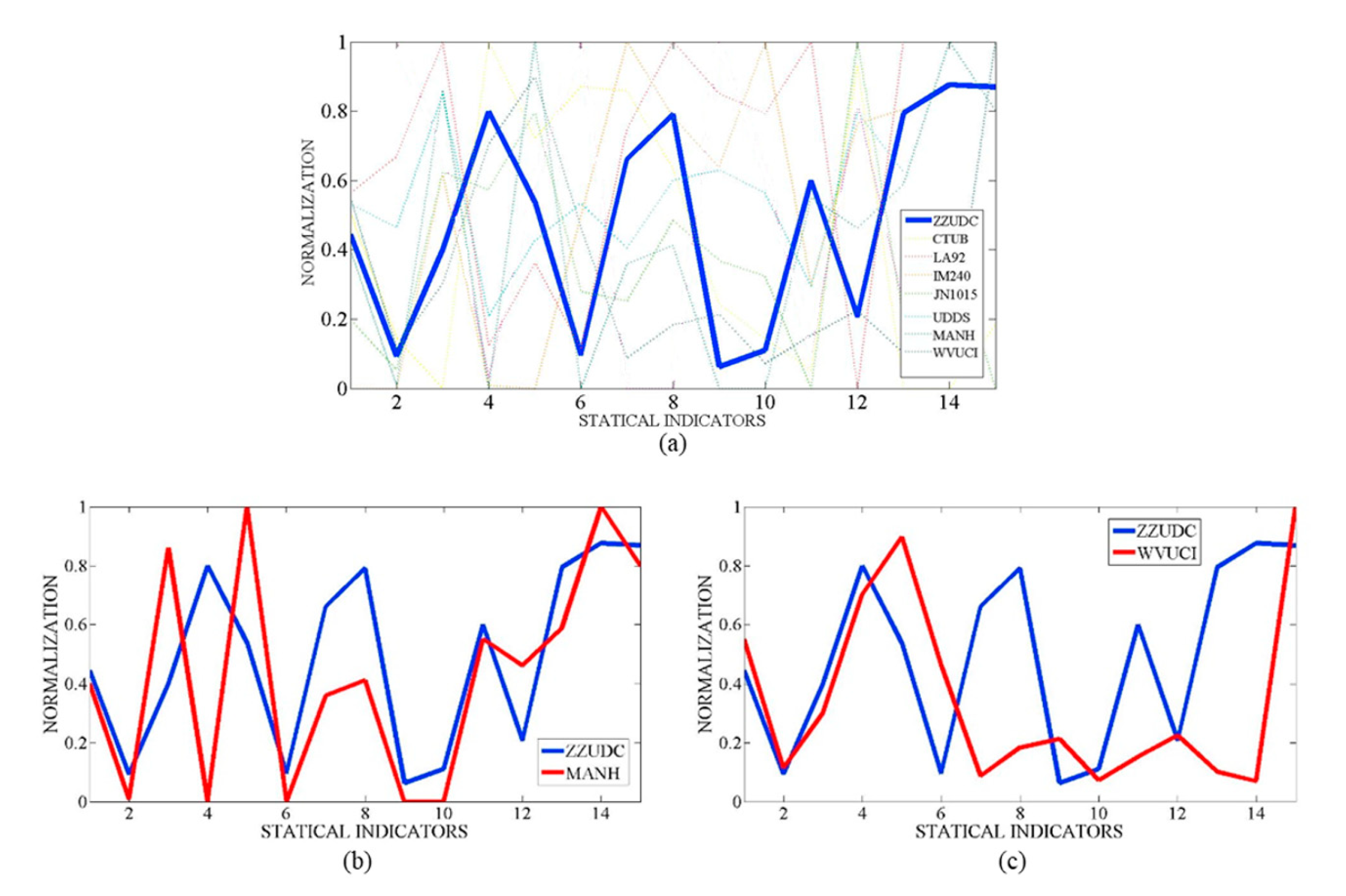
Furthermore, in order to visually depict the relative distributions of all the cycles in every statistical item, we can normalize the figures with every line according to
where is the specific figure in a vector. The results of all the driving cycles are displayed in Figure 11.
The normalization range is between 0 and 1. If most of the figures converge in one certain pole (0 or 1) in any statistical indicator, this indicates that there is a stand-out. However, in Figure 11, the plots of eight cycles, ZZUDC included, are substantially decentralized in every item. Thus, ZZUDC is mediocre, rather than extreme, which verifies the rationality of the cycle. Besides this, as we mentioned before, the characteristics of ZZUDC are similar to those of MANHATTAN and WUVCITY. The trends of their broken lines prove this conclusion. As for the distinction in fuel consumption of ZZUDC and WUVCITY, the dominant reason is that the required power of the bus when it drives on WUVCITY is at a lower level than on ZZUDC, which can be reflected, to some extent, by the summit power.
5.3. Discussion
The validation process of ZZUDC mainly conducted from the perspective of the effectiveness of the construction method and the driving cycle’s statistical items. Firstly, the correlation coefficients of characteristic parameters were computed and VPAD figures were plotted, which indicated that the constructed driving cycle (ZZUDC) largely maintains the original data. Moreover, it is evident that, compared with the traditional micro-trip construction method, ZZUDC reflects most of the original data’s characteristics better. Besides this, among ZZUDC and the other seven international driving cycles, ZZUDC is distributed in the middle of them and similar to MANHATTAN and WVUCITY with respect to the majority of normalized statistical items. Therefore, all results show that the constructed ZZUDC is reasonable and credible.
6. Conclusions
In this study, the driving cycle data of two HEB routes in Zhengzhou city are collected with a measurement system integrating global positioning and inertial navigation function. New methods for velocity fragment division and state cluster distribution, improved PM calculation method, and dynamic programming are applied to develop the Zhengzhou urban driving cycle for HEB. We construct the driving cycle parts separately, namely start part, middle part, and end part. During the construction process, characteristic matrices for each part of the driving cycle are established, using 16 characteristic parameters, including road slope, in which mathematical statistic theories related to Markov chain are used. Then, a special method of PM calculation, including the normalization process, is presented to determine the final driving cycle, which can eliminate the difference that is caused by the non-uniform unit of different characteristic parameters and guarantee the reasonability of velocity fragment selection.
By comparing the correlation coefficients of the driving cycles that are constructed based on Markov and traditional micro-trip, the driving cycle constructed in this paper is confirmed to be more objective and effective, with a higher coefficient with the original data. Furthermore, through analyzing the statistical characteristics of ZZUDC and seven international cycles, the target cycle is proven to be reasonable. As for the energy consumption, the values of ZZUDC and MANHATTAN are similar, combining dynamic programming. To be specific, fuel consumption is around 20.5 L/100 km and electricity consumption is approximately 12.8 kwh/100 km.
The established HEB driving cycle construction approach can provide a reference for developing a driving cycle for HEV that drives in pure electric mode at a low velocity without an idling state. Furthermore, this paper lays the foundation for using dynamic programming to compute fuel consumption and electricity consumption for HEBs. In future research, we will investigate the possibility of developing an energy consumption management strategy to improve HEB emission.
Author Contributions
J.P. and J.J. designed the study, collected the data, and analyzed the data. F.D. and H.T. participated in the data analysis. J.J. and J.P. wrote the manuscript. F.D. and H.T. revised and edited the manuscript. All authors have read and agreed to the published version of the manuscript.
Funding
This research was funded by the National Natural Science Foundation of China (Grant No. 51705020 and No. 61620106002) and in part by the Fundamental Research Funds for the Central Universities (Grant No. 2242020R10045).
Acknowledgments
The authors would like to thank the reviewers and Yang Zhou for their corrections and helpful suggestions.
Conflicts of Interest
The funders had no role in the writing of the manuscript.
References
- Li, L.; Yang, C.; Zhang, Y.; Zhang, L.; Song, J. Correctional DP-based energy management strategy of plug-in hybrid electric bus for city-bus route. IEEE Trans. Veh. Technol. 2014, 64, 2792–2803. [Google Scholar] [CrossRef]
- Nesamani, K.S.; Subramanian, K.P. Development of a driving cycle for intra-city buses in Chennai, India. Atmos. Environ. 2011, 45, 5469–5476. [Google Scholar] [CrossRef]
- Ho, S.H.; Wong, Y.D.; Chang, V.W.C. Developing Singapore Driving Cycle for passenger cars to estimate fuel consumption and vehicular emissions. Atmos. Environ. 2014, 97, 353–362. [Google Scholar] [CrossRef]
- Lien, N.T.Y.; Dung, N.T. The determination of driving characteristics of Hanoi bus system and their impacts on the emission. Vietnam. J. Sci. Technol. 2017, 55, 74. [Google Scholar] [CrossRef] [Green Version]
- Yu, L.; Wang, Z.; Qiao, F.; Qi, Y. Approach to development and evaluation of driving cycles for classified roads based on vehicle emission characteristics. Transp. Res. Rec. 2008, 2058, 58–67. [Google Scholar] [CrossRef]
- André, M. The ARTEMIS European driving cycles for measuring car pollutant emissions. Sci. Total Environ. 2004, 334–335, 73–84. [Google Scholar] [CrossRef]
- Lee, C.P. Development of Driving Cycles for Characterizing Vehicular Emission Factors; Hong Kong Polytechnic University: Hong Kong, China, 2006. [Google Scholar]
- Jiang, P.; Shi, Q.; Chen, W.; Huang, Z.A. A research on the construction of city road driving cycle based on wavelet analysis. Automot. Eng. 2011, 69–70. [Google Scholar]
- Berzi, L.; Delogu, M.; Pierini, M. Development of driving cycles for electric vehicles in the context of the city of Florence. Transp. Res. Part. D Transp. Environ. 2016, 47, 299–322. [Google Scholar] [CrossRef]
- Li, Y.; He, H.; Peng, J. An adaptive online prediction method with variable prediction horizon for future driving cycle of the vehicle. IEEE Access 2018, 6, 33062–33075. [Google Scholar] [CrossRef]
- Shi, S.; Lin, N.; Zhang, Y.; Cheng, J.; Huang, C.; Liu, L.; Lu, B. Research on Markov property analysis of driving cycles and its application. Transp. Res. Part. D Transp. Environ. 2016, 47, 171–181. [Google Scholar] [CrossRef]
- Lin, J. A Markov Process Approach to Driving Cycle Development; University of California, Davis: Davis, CA, USA, 2020. [Google Scholar]
- Lee, T.K.; Adornato, B.; Filipi, Z.S. Synthesis of real-world driving cycles and their use for estimating PHEV energy consumption and charging opportunities: Case study for midwest/U.S. IEEE Trans. Veh. Technol. 2011, 60, 4153–4163. [Google Scholar] [CrossRef]
- Lee, T.C.; Judge, G.G.; Zellner, A. Estimating the Parameters of the Markov Probability Model from Aggregate Time Series Data; North-Holland: Amsterdam, The Netherlands, 1970. [Google Scholar]
- Liu, L.; Huang, C.; Lu, B.; Shi, S.; Zhang, Y.; Cheng, J. Study on the design method of time-variant driving cycles for EV based on Markov Process. In Proceedings of the 2012 IEEE Vehicle Power and Propulsion Conference, Seoul, Korea, 9–12 October 2012; pp. 1277–1281. [Google Scholar]
- Zhang, M.; Shi, S.; Lin, N.; Yue, B. High-efficiency driving cycle generation using a Markov chain evolution algorithm. IEEE Trans. Veh. Technol. 2018, 68, 1288–1301. [Google Scholar] [CrossRef]
- Fontaras, G.; Franco, V.; Dilara, P.; Martini, G.; Manfredi, U. Development and review of Euro 5 passenger car emission factors based on experimental results over various driving cycles. Sci. Total. Environ. 2014, 468–469, 1034–1042. [Google Scholar] [CrossRef] [PubMed]
- Lin, J.; Niemeier, D.A. Estimating regional air quality vehicle emission inventories: Constructing robust driving cycles. Transp. Sci. 2003, 37, 330–346. [Google Scholar] [CrossRef] [Green Version]
- Pang, W.K.; Yang, Z.H.; Hou, S.H.; Leung, P.K. Non-uniform random variate generation by the vertical strip method. Eur. J. Oper. Res. 2002, 142, 595–609. [Google Scholar] [CrossRef]
- Eisinger, D.S.; Niemeier, D.A.; Stoeckenius, T.; Kear, T.P.; Brady, M.J.; Pollack, A.K.; Long, J. Collecting Driving Data to Support Mobile Source Emissions Estimation. J. Transp. Eng. 2006, 132, 845–854. [Google Scholar] [CrossRef]
- Esteves-Booth, A.; Muneer, T.; Kirby, H.; Kubie, J.; Hunter, J. The measurement of vehicular driving cycle within the city of Edinburgh. Transp. Res. Part. D Transp. Environ. 2001, 6, 209–220. [Google Scholar] [CrossRef]
- Wirasingha, S.G.; Emadi, A. Classification and review of control strategies for plug-in hybrid electric vehicles. IEEE Trans. Veh. Technol. 2010, 60, 111–122. [Google Scholar] [CrossRef]
- Shen, P.; Zhao, Z.; Li, J.; Zhan, X. Development of a typical driving cycle for an intra-city hybrid electric bus with a fixed route. Transp. Res. Part. D Transp. Env. 2018, 59, 346–360. [Google Scholar] [CrossRef]
- He, K.; Zhu, Z.F. Code for Design of Urban Road Engineering. China Architecture & Building Press: Beijing, China, 2012. [Google Scholar]
- Abou-Nasr, M.; Michelini, J.; Filev, D. Real World Data Mining Applications; Springer International Publishing: Cham, Switzerland, 2015; pp. 343–358. [Google Scholar]
- Hung, W.T.; Tong, H.Y.; Lee, C.P.; Ha, K.; Pao, L.Y. Development of a practical driving cycle construction methodology: A case study in Hong Kong. Transp. Res. Part. D Transp. Environ. 2007, 12, 115–128. [Google Scholar] [CrossRef]
- Fotouhi, A.; Montazeri-Gh, M. Tehran driving cycle development using the k-means clustering method. Sci. Iran. 2013, 20, 286–293. [Google Scholar]
- Peng, J.; Fan, H.; He, H.; Pan, D. A Rule-Based Energy Management Strategy for a Plug-in Hybrid School Bus Based on a Controller Area Network Bus. Energies 2015, 8, 5122–5142. [Google Scholar] [CrossRef] [Green Version]
- Peng, J.; He, H.; Xiong, R. Rule based energy management strategy for a series—Parallel plug-in hybrid electric bus optimized by dynamic programming. Appl. Energy 2017, 185, 1633–1643. [Google Scholar] [CrossRef]
Figure 1.
Flow chart of driving cycle construction based on Markov process.

Figure 2.
Route schematic: (a) Route of BRT B17; (b) Route of traditional bus 906.

Figure 3.
Partial road slope filtering results.

Figure 4.
Velocity fragment division based on velocity threshold.

Figure 5.
Basis for fragment division.

Figure 6.
Variation trend of difference matrixes’ F norm.

| State 1 | State 2 | State 3 | State 4 | State 5 | State 6 | State 7 | Total | |
|---|---|---|---|---|---|---|---|---|
| State 1 | 7430 | 1878 | 508 | 167 | 14 | 0 | 0 | 9997 |
| Probability | 0.7432 | 0.1879 | 0.0508 | 0.0167 | 0.0014 | 0 | 0 | 1 |
| … | ||||||||
| Probability |
Figure 7.
Urban driving cycle of hybrid electric bus.

Figure 8.
Distance–slope curve of driving cycle.

Figure 9.
Comparison of VAPDs: (a) VAPD of the original data. (b) VAPD of the constructed driving cycle.
Figure 9.
Comparison of VAPDs: (a) VAPD of the original data. (b) VAPD of the constructed driving cycle.

Figure 10.
Comparison of driving cycle construction results.

Figure 11.
Normalization results: (a) normalizations of 8 cycles in 15 statistical items; (b) normalizations of ZZUDC and MANHATAN; (c) normalizations of ZZUDC and WVUCITY.
Figure 11.
Normalization results: (a) normalizations of 8 cycles in 15 statistical items; (b) normalizations of ZZUDC and MANHATAN; (c) normalizations of ZZUDC and WVUCITY.


Table 1.
The selected bus test route.
| Route | B17 | 906 |
|---|---|---|
| Single transit operation distance | 15 km | 21 km |
| Bus stops | 27 | 36 |
| Single transit operation time | 2.5–3 h | 3.5–4 h |
| Test acquisition time | 7:00–9:00; 10:00–12:00; 16:00–18:00 | 7:00–11:00; 14:00–18:00 |
Table 2.
Specific parameters of test bus.
| Parameters | Values | Parameters | Values |
|---|---|---|---|
| Length | 12.0 m | Engine displacement | 6494 mL |
| Width | 2.55 m | Engine rated power | 155/2500 kW/rpm |
| Height | 3.05 m | Traction motor rated power | 95/1800 kW/rpm |
| Wheel base | 6.10 m | Maximum velocity | 85 km/h |
| Outfit quality | 12,400 kg | Capacity of power battery packs | 72 Ah |
Table 3.
Probability distribution of sampling points in low velocity.
| Velocity (km/h) | 0–0.4 | 0.4–0.7 | 0.7–1 | 1–1.5 | 1.5–2 | 2–2.5 | 2.5–3 | 3–3.5 | 3.5–4 |
| Probability Distribution (%) | 50.01 | 17.32 | 9.36 | 7.85 | 4.70 | 3.36 | 2.80 | 2.42 | 2.20 |
Table 4.
Probability distribution of sampling points in stop fragments.
| Acceleration Absolute Value | 0–0.05 | 0.05–0.1 | 0.1–0.15 | 0.15–0.2 | 0.2–0.25 | 0.25–0.3 | 0.3–0.35 | >0.35 |
| Probability Distribution (%) | 82.09 | 9.92 | 2.59 | 1.23 | 0.75 | 0.60 | 0.49 | 2.33 |
Table 5.
The moments and probabilities of transfer events from state 1.
| State 1 | State 2 | State 3 | State 4 | State 5 | State 6 | State 7 | Total | |
|---|---|---|---|---|---|---|---|---|
| State 1 | 7430 | 1878 | 508 | 167 | 14 | 0 | 0 | 9997 |
| Probability | 0.7432 | 0.1879 | 0.0508 | 0.0167 | 0.0014 | 0 | 0 | 1 |
| … | ||||||||
| Probability |
Table 6.
Characteristic parameters of original data.
| No. | Characteristic Parameters | Statistic | No. | Characteristic Parameters | Statistic |
|---|---|---|---|---|---|
| 1 | Proportion of stop time | 24.09% | 9 | Maximum acceleration | 4.507 |
| 2 | Proportion of uniform time | 19.91% | 10 | Acceleration standard deviation | 0.5944 |
| 3 | Proportion of acceleration time | 30.31% | 11 | Minimum slope | −4.59° |
| 4 | Proportion of deceleration time | 25.69% | 12 | Maximum slope | 5.61° |
| 5 | Velocity standard deviation | 13.67 | 13 | Average slope | 0.54° |
| 6 | Maximum velocity | 53.762 | 14 | Minimum road power | −32.6027 |
| 7 | Average velocity | 14.8962 | 15 | Maximum road power | 627.1849 |
| 8 | Minimum acceleration | −5.399 | 16 | Average road power | 24.7528 |
Table 7.
PM values of 3 candidate parts.
| PM Values Sorted by Size | PM Values of Candidate Start Parts | PM Values of Candidate Middle Parts | PM Values of Candidate End Parts |
|---|---|---|---|
| 1 | 2.510540671 | 4.739681266 | 2.501163991 |
| 2 | 2.569868781 | 7.319837123 | 2.737829385 |
| 3 | 2.628233751 | 8.021323306 | 3.613194073 |
| 4 | 2.653348204 | 8.472976857 | 4.692183328 |
| 5 | 2.668761563 | 9.019943662 | 4.924311752 |
| 6 | 2.945562042 | 9.504009244 | 5.055707237 |
| 7 | 3.040904642 | 9.904238173 | 5.510211213 |
| 8 | 3.257100981 | 10.28213778 | 6.020786659 |
| 9 | 3.285076105 | 10.68241299 | 7.054115036 |
| 10 | 3.327682241 | 11.13303276 | 7.404858184 |
| …… | |||
| 912 | 7.463476789 | ||
| 923 | 7.508530394 |
Table 8.
Comparison of characteristic parameters.
| Characteristic Parameters | Original Data | Markov | Micro-Trip |
|---|---|---|---|
| Proportion of stop time | 24.09% | 22.93% | 32.51% |
| Proportion of uniform time | 19.91% | 14.97% | 16.80% |
| Proportion of acceleration time | 30.31% | 33.32% | 27.30% |
| Proportion of deceleration time | 25.69% | 28.78% | 23.39% |
| Velocity standard deviation | 13.67 | 13.556 | 13.742 |
| Maximum velocity | 53.762 | 49.634 | 48.489 |
| Average velocity | 14.896 | 14.961 | 13.688 |
| Minimum acceleration | −5.399 | −5.399 | −2.777 |
| Maximum acceleration | 4.507 | 4.031 | 2.459 |
| Acceleration standard deviation | 0.594 | 0.700 | 0.542 |
| Minimum slope | −5.154 | −3.398 | −4.888 |
| Maximum slope | 5.152 | 4.789 | 4.762 |
| Average slope | 0.021 | −0.233 | −0.486 |
| Minimum road power | −32.602 | −32.603 | −31.314 |
| Maximum road power | 308.165 | 217.185 | 137.080 |
| Average road power | 24.753 | 26.871 | 21.619 |
Table 9.
Zhengzhou urban driving cycle and international urban driving cycles.
| Statistical items | ZZUDC | CTUB | LA92 | IM240 | JN1015 | UDDS | MANHATTAN | WVUCITY |
|---|---|---|---|---|---|---|---|---|
| Time (s) | 1184 | 1314 | 1436 | 241 | 661 | 1370 | 1090 | 1408 |
| Mileage (km) | 4.919 | 5.898 | 15.797 | 3.152 | 4.164 | 11.921 | 3.324 | 5.319 |
| Average acc. (m/s2) | 0.459 | 0.299 | 0.699 | 0.5452 | 0.548 | 0.6375 | 0.6432 | 0.4201 |
| Average dec. (m/s2) | −0.512 | −0.431 | −0.787 | −0.833 | −0.604 | −0.752 | −0.836 | −0.551 |
| Idling proportion (%) | 22.93 | 29.00 | 17.061 | 4.979 | 31.467 | 19.197 | 38.349 | 34.943 |
| Uniform proportion (%) | 14.97 | 36.606 | 15.460 | 26.141 | 20.121 | 27.226 | 12.294 | 25.213 |
| Acc. proportion (%) | 33.32 | 37.367 | 35.097 | 40.249 | 24.962 | 28.102 | 27.156 | 21.591 |
| Dec. proportion (%) | 28.78 | 26.027 | 32.382 | 28.631 | 23.449 | 25.474 | 22.202 | 18.253 |
| Maximum velocity (km/h) | 45.634 | 60 | 108.15 | 91.25 | 69.97 | 90.72 | 40.71 | 57.65 |
| Average velocity (km/h) | 14.961 | 16.16 | 39.60 | 47.08 | 22.68 | 31.32 | 10.98 | 13.60 |
| Maximum acc. (m/s2) | 2.167 | 0.914 | 3.085 | 1.4752 | 0.7933 | 1.4667 | 2.0559 | 1.1433 |
| Minimum dec. (m/s2) | −3.292 | −1.042 | −3.934 | −1.565 | −0.833 | −1.467 | −2.503 | −3.237 |
| RMS1 of acc. (m/s2) | 0.700 | 0.333 | 0.795 | 0.705 | 0.424 | 0.621 | 0.605 | 0.380 |
| Fuel consumption (L/100 km) | 20.509 | 14.985 | — | — | 17.710 | — | 21.288 | 15.419 |
| Electricity consumption (kwh/100 km) | 12.772 | 9.8581 | — | — | 9.081 | — | 12.474 | 13.326 |
1 Root mean square.
© 2020 by the authors. Licensee MDPI, Basel, Switzerland. This article is an open access article distributed under the terms and conditions of the Creative Commons Attribution (CC BY) license (http://creativecommons.org/licenses/by/4.0/).
Share and Cite
MDPI and ACS Style
Peng, J.; Jiang, J.; Ding, F.; Tan, H. Development of Driving Cycle Construction for Hybrid Electric Bus: A Case Study in Zhengzhou, China. Sustainability 2020, 12, 7188. https://0-doi-org.brum.beds.ac.uk/10.3390/su12177188
AMA Style
Peng J, Jiang J, Ding F, Tan H. Development of Driving Cycle Construction for Hybrid Electric Bus: A Case Study in Zhengzhou, China. Sustainability. 2020; 12(17):7188. https://0-doi-org.brum.beds.ac.uk/10.3390/su12177188
Chicago/Turabian StylePeng, Jiankun, Jiwan Jiang, Fan Ding, and Huachun Tan. 2020. "Development of Driving Cycle Construction for Hybrid Electric Bus: A Case Study in Zhengzhou, China" Sustainability 12, no. 17: 7188. https://0-doi-org.brum.beds.ac.uk/10.3390/su12177188
Note that from the first issue of 2016, this journal uses article numbers instead of page numbers. See further details here.