Sanitation Network Sulfide Modeling as a Tool for Asset Management. The Case of the City of Murcia (Spain)

Abstract

Hydrogen sulfide (H₂S) generated in sewer networks induces corrosion which today constitutes the main cause of deterioration of concrete pipes. Information regarding the H₂S concentration inside sewer networks, as well as its control and reduction, has become one of the most important concerns in sanitation systems management nowadays. Modeling sulfide dynamics is the key to understanding corrosion processes. A dynamic model (called EMU-SANETSUL) was developed to calculate the H₂S concentration in both the water and the gas phases of the main sewers of the city of Murcia (Spain). The model was calibrated with data from field measurements taken from both the gas phase and wastewater. Samples were taken in the network from 2016 to 2019. The model achieved an accuracy index and error index in the ranges of 57% and 15%, respectively. Empirical equations of reaction are used, and calibration parameters are detailed. The code uses an explicit discretization technique, named the Discrete Volume Element Method (DVEM). A map with the annual average concentration of H₂S at the gas phase inside each pipe of the simulated network is presented. Values are compared with the mechanical deterioration inventory from closed-circuit television (CCTV) inspections performed by the Municipal Sanitation Company of the city of Murcia (EMUASA). Mechanical deterioration of pipes has diverse causes, including corrosion of pipes by H₂S. Sections with high H₂S concentrations that match with mechanical wear can be considered susceptible to being prioritized when rehabilitation works are being planned. Therefore, H₂S concentration modeling provides valuable information for asset management of the sewer network.

1. Introduction

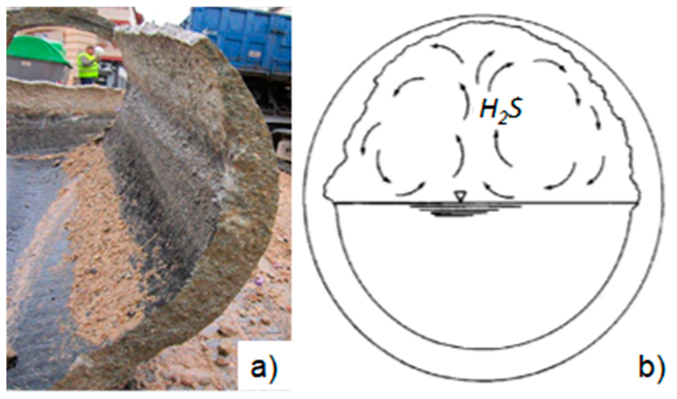
Hydrogen sulfide, H₂S, is a gas generated in wastewater due to the reduction of sulfate to sulfide, as a result of the sulfate reducing bacteria (SRB) in anaerobic sewer biofilms. In the sulfate reduction process sulfides are formed, consisting of H₂S, HS⁻, and S₂⁻, where the distribution between these sulfide species depends on the pH [1,2]. Hydrogen sulfide has a low solubility in water, and turbulence causes it to be released into the gas phase of the pipes at concentrations that may be harmful to people working in the sewage systems. In addition, this gas causes significant complaints of bad odors when it reaches street level. Another important problem is due to the formation of sulfuric acid, which favors the degradation of concrete pipes by neutralizing the alkalinity of the concrete and by the formation of expansive salts with no binding properties, which can cause internal cracking at the concrete interface. Moreover, iron corrosion occurs in reinforced concrete pipes. Figure 1 shows a pipe suffering from this degradation phenomenon in the city of Murcia. Once anaerobic conditions (<0.1 mg/L of dissolved oxygen) are reached inside the pipe, some of the main factors influencing the formation of sulfides in wastewater as it passes through the sewer networks are the following: (1) organic load transported by the water in dry weather, BOD₅; (2) wastewater temperature; (3) hydraulic retention time (HRT); and (4) hydraulic conditions of flow, such as velocity, wetted perimeter, or percentage of filling of the pipe [3,4,5].

Hydrogen sulfide generated in the sewer networks induces corrosion, which is the main cause of deterioration of concrete pipes today [1,6,7]. The costs associated with the replacement of corroded pipes and the application of corrosion inhibitors amount to billions of dollars annually [6]. In March 2000, the annual total cost attributed to corrosion in sewer systems of the United States was estimated to be $13.75 billion [6,8]. The water and sanitation administrations and utilities are aware and concerned about the deterioration of these assets and are committed to intensifying inspections in the sanitation networks and in establishing prioritization in the renewal of pipes based on their state of corrosion and mechanical deterioration [9,10,11,12]. 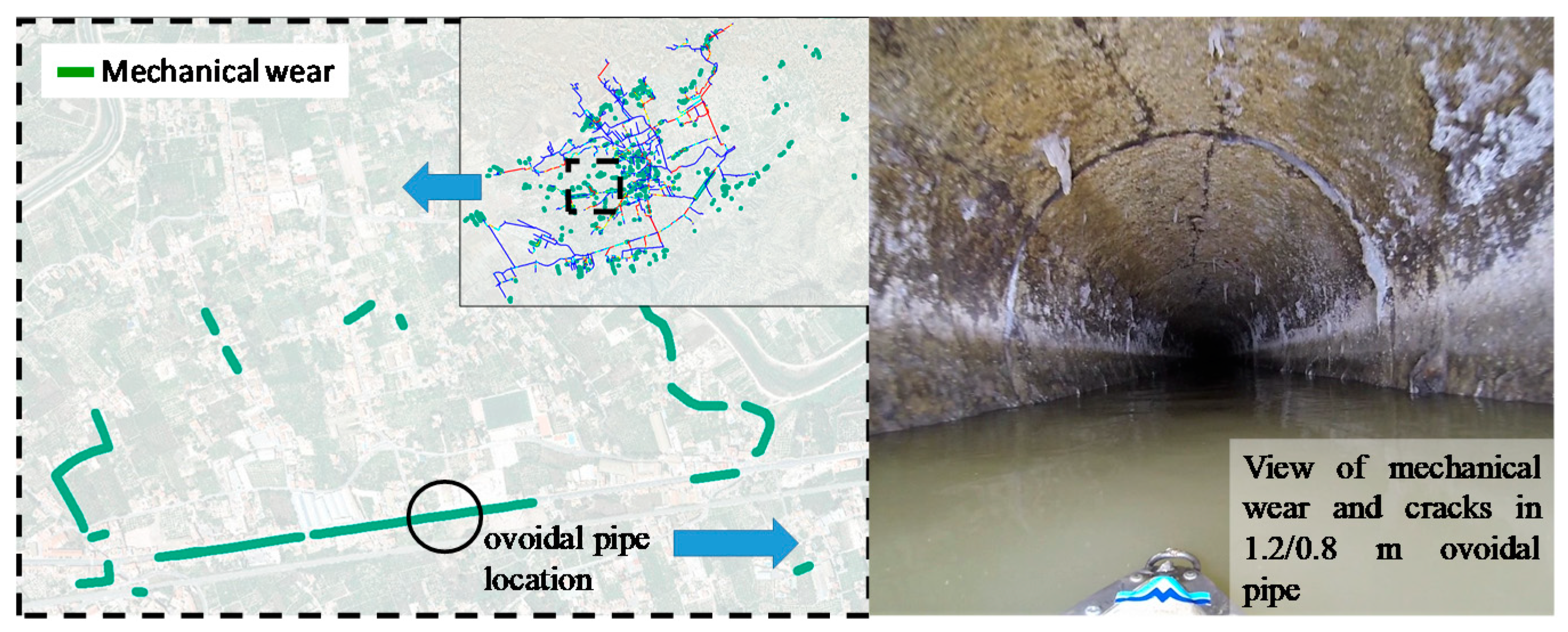Techniques to protect pipes through inner coatings of the in-sewers are particularly important [13]. In the case of the Municipal Sanitation Utility of Murcia (EMUASA), maps are prepared based on CCTV inspections of the pipes where mechanical deterioration is observed. Such information is used in the process of prioritizing pipeline renewal (Figure 2).

Mechanical deterioration refers to the loss of wall thickness, due to biochemical corrosion, to any crack that could be due to external traffic load or any other cause of deterioration that could be observed thorough visual inspection.

Thus, knowing the concentration of H₂S inside sewerage networks, as well as its control and reduction, has become one of the main concerns in sewerage system management nowadays [14]. Online and continuous monitoring of H₂S concentrations in sewers has been demonstrated as a useful technique in understanding and slowing the deterioration of concrete pipes [15,16,17]. The dosing of chemicals into the sewerage network to reduce the H₂S concentration is a common practice, especially during the summer periods and in coastal areas. Continuous monitoring has shown the possibility of optimizing and reducing the chemicals used in sewers [18].

Modeling sulfide dynamics over time in the water and air phases in sewer networks is of great importance to understand corrosion processes. Deterministic simulation models are used in order to predict H₂S concentrations, dissolved and in the gas phase inside the pipe. Such models can be based on the mass balance equations considering kinetics and stoichiometric of the processes, and require knowledge of a high number of parameters, such as the WATS model (2013, HV-Consult ApS, Aalborg, Denmark) [3,19,20]. However, empirical models, with a lower number of parameters, also propose a balance based on various factors, such as the organic load and the hydraulic conditions of flow, reaching, in some cases, a sufficient approximation to values measured in the field [21,22,23,24,25,26,27,28,29]. Three principal processes occur in the sewers and must be simulated: (1) sulfide generated in the biofilm in the contact area between the wastewater and the concrete pipe; (2) emission to the sewer gas phase inside the pipe; and (3) absorption of hydrogen sulfide through the concrete pipe.

Regarding empirical models, Pomeroy and Parkhurst [22] presented an empirical equation for sulfide generation based on biochemical oxygen demand at five days. Boon and Lister [23] proposed a similar generation equation based on the chemical organic demand (COD). Elmaleh et al. [24] showed the production of sulfide in the pipeline from an installation of 61 km in length that transported recycled urban water by gravity and in full section. Yongsiri et al. [25,26] proposed a model of H₂S emissions in gravity pipelines considering two phases (liquid and air) with generation and emission. Lahav et al. [27] proposed an approximation of H₂S emissions through a first order kinetic equation based on laboratory tests, using flocculation equipment to provide different degrees of turbulence to the experiments. Other authors such as [28,29] considered an extension of the WATS model, proposing different equations for each of the processes that generate the sulfur cycle in a sanitation system. Nielsen et al. [30] presented a hydraulic model that analyzes the generation and emission from equations previously developed by [22] and [3] to study the influence of chemical dosing. Recently, studies of H₂S gas modeling with WATS have been presented by Vollertsen et al., 2015 [31], for a large area of the city of San Francisco. Matias et al. [32] modeled the Ericeira sewer system in Portugal, using WATS and AEROSEPT models, and adequately predicted the overall behavior of the system. Nowadays, several commercial software packages are available for modeling sulfide concentrations [19,33,34].

Several researchers have studied the influence of sulfide corrosion on the life-cycle of the pipes [35]. For instance, Teplý et al. [36] proposed an approach to calculate a service-life prognosis that considers the influence of microbiologically induced corrosion (MIC) on bearing capacity. When corrosion is sufficiently advanced, it leads to diminished service life or structural failures. Zamanian et al. [37] used computational numerical models to study the effects of a number of key modeling and construction factors on the leakage susceptibility of buried concrete sewer pipes. These factors included the loss of pipe wall due to the corrosion process as a function of time. The sensitivity analysis carried out by Mahmoodian and Li [38] showed that the supplied concentration of sulfide and the relative depth of the fluid have significant effects on the service life of concrete sewer pipes. Ahammed and Melchers [39] proposed a corrosion model to calculate the loss of pipe wall thickness with time. They used 20 independent random variables that included the geometric characteristics of pipes (including the radius and the wall thickness, among others), mechanical and load characteristics (such as the modulus of elasticity Poisson’s ratio and traffic loads), ditch construction characteristics (external soil and width, etc.), and temperature differential among others. Once the concentration of hydrogen sulfide in a sewer network can be predicted and the loss of wall thickness through corrosion can be calculated, this will lead to being able to establish the level of service of the pipes and this would make it possible to plan the renewal and management of assets in a more sustainable way.

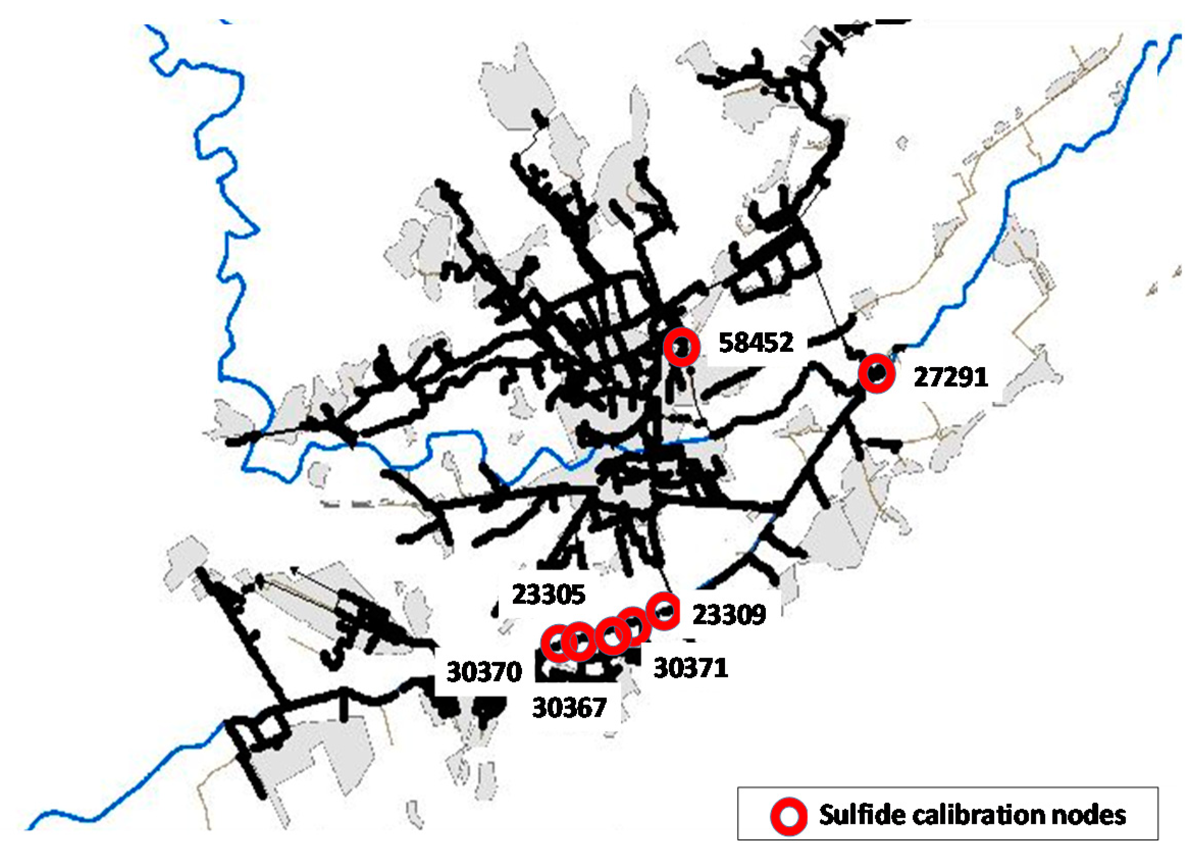
In the present work, a dynamic model (called EMU-SANETSUL) was developed to calculate the H₂S concentration in both the water and air phases of the main sewers of the city of Murcia. This wastewater network mainly contains domestic and commercial sanitary sewage. The model is calibrated with data from field measurements. One-dimensional time-variation hydraulic variables and H₂S reactions are solved using an explicit discretization technique called the Discrete Volume Element Method (DVEM) [40,41,42]. That scheme is based on a mass-balance relation within pipes that considers both advective transport as well as reaction kinetics of sulfides in the water and air phases. The reaction uses empirical equations included in [21]. For this purpose, we start from an existing calibrated hydraulic model of the Municipal Water and Sanitation Company of Murcia (EMUASA) [43,44]. From the simulated H₂S concentrations in the gas phase inside the pipe of the main sewer network of the city of Murcia, this study provides a map showing the sections with higher sulfide concentrations. This information, together with the mechanical wear inventory, provides valuable information for the asset management of sewers, helping in the planning and prioritization of pipe renovation and rehabilitation. The objective of the present work is to provide information on the H₂S concentration in the air phase of the sewers. This information may serve to predict the pipes with high risk of corrosion and it will help in decision-making in asset management as one more variable.

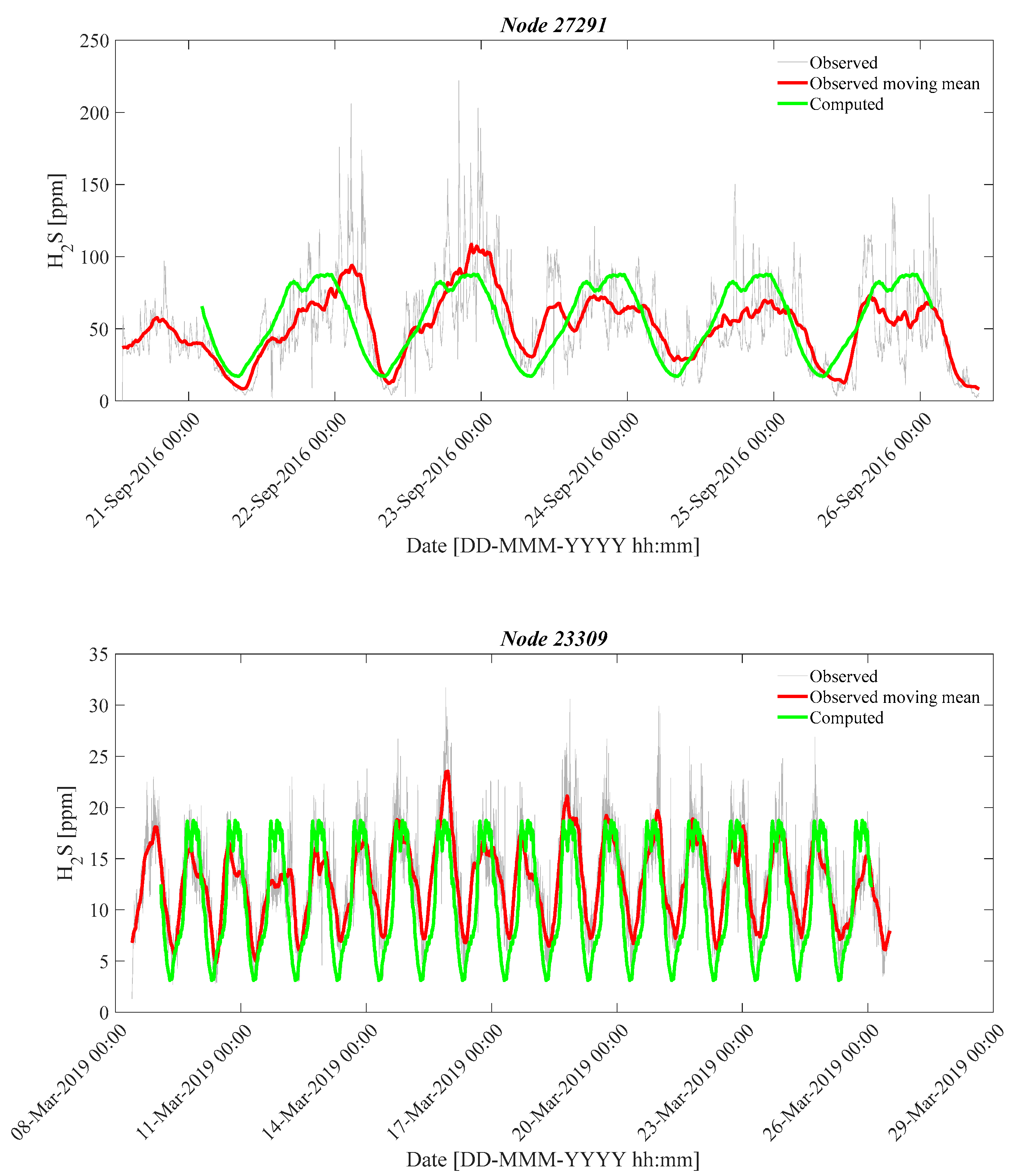
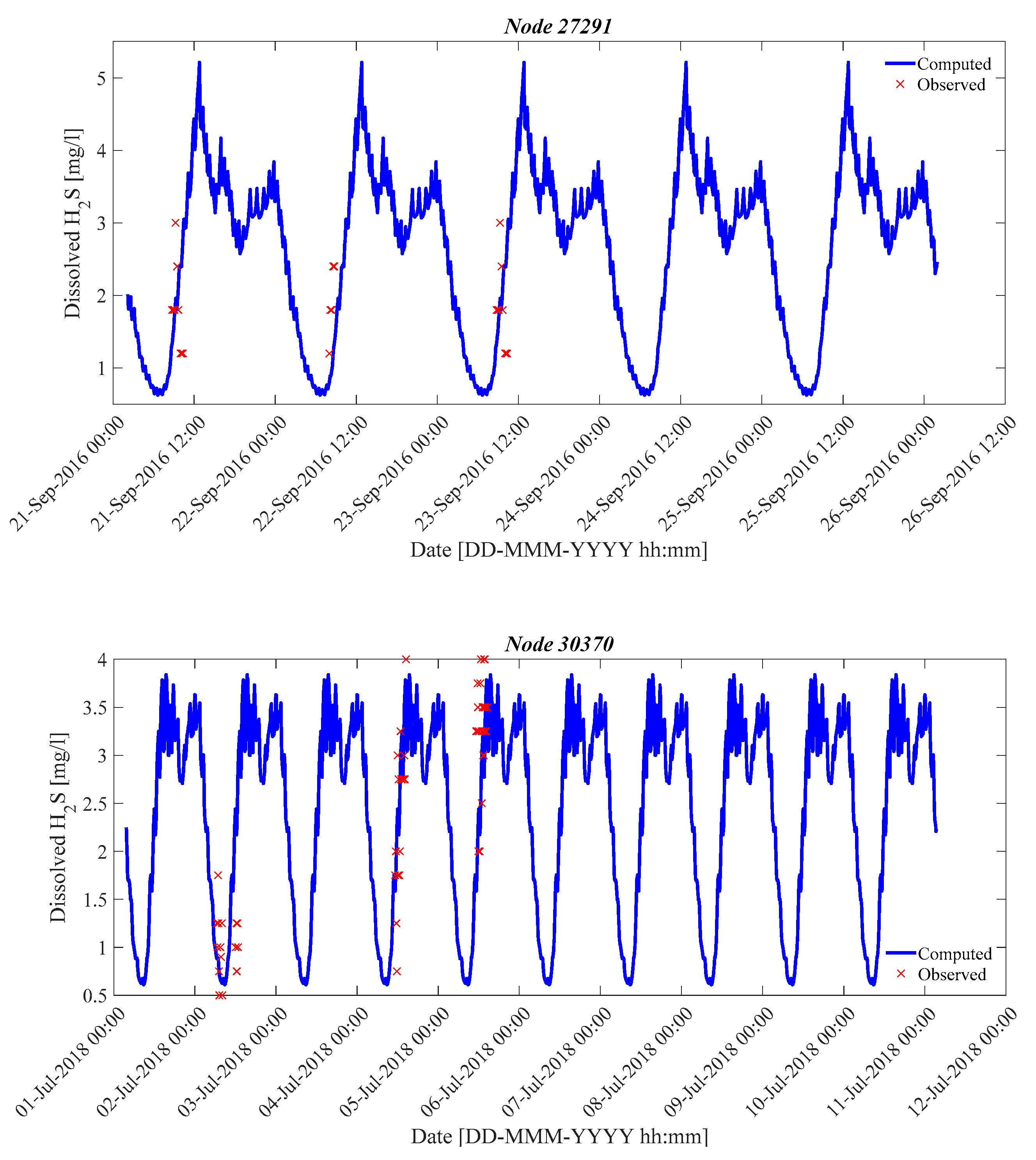
2. Materials and Methods

2.1. Hydraulic Model of Reference

Murcia is a city in southeastern Spain whose municipality has a population of 453,258 inhabitants. It is situated in a valley at the confluence of the Guadalentín and Segura rivers. The sewer system is combined and incorporates storm water. Due to the nearly no-slope topographic conditions, there are several sewer pump stations. Sewers flow into the “Murcia Este” Wastewater Treatment Plant (WWTP) with a maximum capacity during dry weather of Q_maxdw = 10,000 m³/h. Along the network, there are 57 control points consisting of a water gauge to continuously monitor the water level with Endress + Hauser FMR50 ultrasonic sensors. Data are sent continuously and plotted through a SCADA system at five-minute intervals. The Storm Water Management Model SWMM (2020, Environmental Protection Agency EPA, Durham, NC, USA) is a numerical model that enables the hydrological and hydraulic behavior of an urban drainage system to be simulated. A previously calibrated SWMM hydraulic model of the city of Murcia is available [43,45]. The model includes the main sewers of the whole sewer network. It serves to study the transport of dry-weather wastewater flows throughout the day to the WWTP (Figure 3). The main characteristics of the model are shown in

Table 1. Description of the hydraulic model of Murcia.

Description	Element	Number
Hydraulics	Nodes	6656
	Outfalls	65
	Tanks	65
	Links	6655
	Pump stations	39

. The total length of the network included in the model is around 234.5 km. The comparison of the measured and simulated flow depth is shown in Supplementary Materials, Figure S1. The whole system considered in the present work is made of concrete pipes.

2.2. Experimental Field Campaign in the City of Murcia

During the periods of September to November 2016, June to July 2018, and February to April 2019, a field campaign was carried out at various mains of the network of the city of Murcia (Spain) that were the responsibility of EMUASA. It consisted in the installation of two continuous H₂S meters to measure the gas phase sulfide concentration with an Odalog detector (LL-H₂S-0-1000, App-Tek International Pty Ltd, Brendale, Australia) with a measurement range of 0–1000 ppm and a resolution of 1 ppm. These units have a battery life of more than 20 days and have a data logger inside which, depending on the frequency of measurements, can also be used for several days. In the present study, a measurement was recorded every five minutes. Samples of wastewater were taken in the closest manholes to the measurement area, with the total acid-soluble sulfide being quantified using the methylene blue methodology. The sulfides react with dimethyl-p-phenylenediamine in the presence of ferric chloride to produce methylene blue. CHEMetrics^® colorimetric kits (sulfides, CHEMetrics Inc., Midland, VA, USA) were used for that purpose (USEPA, 1998). To minimize stripping during the sampling, a two-liter bucket was filled with a peristaltic pump whose intake was located at the bottom of the manhole. To avoid any issue with conservation, the samples were analyzed immediately after being taken. The CHEMetrics^® sulfide test kits were used in the field campaigns. These kits consist of self-filling ampoules for visual colorimetric analysis. The ampoules contain an activator solution based on stable reagents vacuum-sealed. Once the tip gets broken inside a sample cup of 25 mL, part of the raw water, enters the ampoule and reacts with the reagent to form a color reaction. The results are compared with a color pattern to obtain quick quantitative test results. Sampling of wastewater entering from outer nodes to the main system gave rise to H₂S values in the range of 0.1 mg/L which were adopted for the incoming flow.

Prior to the experimental campaign, information was collected at several points of the main sewer network by EMUASA: temperature in the wastewater, and the five-day biochemical oxygen demand curve (BOD₅) in the wastewater transported in the network throughout the day. Figure 4 shows the daily curves for these variables that were to be later used for the wastewater that is transported through the network when applying the dynamical model. Temperature daily curves change depending on the season of the year. From the field measurements, three temperature curves were then used in the present work: February, July, and September–October curves, while only one BOD₅ daily curve is used, as presented in Figure 5. In addition to daily BOD₅ sampling and analysis campaigns, a multiparametric probe (HI-9828, Hanna Instruments Inc., Woonsocket, RI, USA) was also placed in the measurement area. This probe characterizes various physical–chemical and electrical properties of the wastewater, such as dissolved oxygen in the wastewater, oxidation-reduction potential (ORP), electrical conductivity (EC), temperature (T), degree of acidity or basicity (pH), and total dissolved solids (TDS) at both points. In the present work, the probe was principally used to generate the temperature curves. A dissolved oxygen measurement below 0.5 mg/L is an indicator that anaerobic conditions are beginning to govern reactions within the wastewater. In general, the measured values were below 0.1 mg/L.

2.3. Equations and Algorithm That Conform the EMU-SANETSUL Code

2.3.1. Reaction Equations Based on the Empirical Model Proposed by Matos et al.

In the present work, the empirical equations proposed by Matos et al. [21] were adapted for their integration in the novel dynamical code EMU-SANETSUL. The empirical equations included by Matos et al. [21] take a number of equations from other classical empirical models in the field [46,47,48]. The code is composed of two main equations. The first one calculates the H₂S balance in the wastewater; whilst the second one solves the H₂S balance in the gas phase of the collector. Both equations are coupled. The equations and the explanations of its terms are included in the Appendix A.

2.3.2. Discrete Volume Element Method (DVEM)

DVEM is an explicit dynamic water-quality modeling algorithm developed for tracking dissolved substances in water-distribution networks [40]. It assumes that the longitudinal dispersion is neglected. The algorithm is based on a mass-balance equation that accounts for both advective transport and reaction kinetics. This is a one-dimensional transport model with instantaneous cross-sectional mixing. The inputs to the model consist of a topological description of the network, a description of how the hydraulic conditions in the network change over time (from the SWMM hydraulic calibrated model), a reaction rate expression for the constituent of concern, an initial distribution of the constituent throughout the network, and a description of the constituent concentrations entering the network through external source flows over time.

Sulfide mass is allocated to discrete volume elements within each pipe, and within each time step, reactions occur within each element, mass is transported between elements, and mass and flow volumes are mixed at downstream nodes. Each link in the network is divided into a number of equal-sized elements, n, spaced evenly along the link axis. A time step, τ, is selected to ensure that water is not transported in a link beyond its downstream boundary node, a link’s volume element must be chosen to be less than or equal to the flowrate multiplied by the time step, Q_iτ, and τ cannot be greater than the shortest travel time through any of the network links associated with a particular hydraulic event. The following equations detail the time step and number of divisions of the link calculation:

$$\tau =min\left(\frac{Volum{e}_i}{Q_i}\right),$$

(1)

$$n=\left[\frac{Volum{e}_i}{Q_i\tau }\right].$$

(2)

when all the network links have been partitioned into volume elements and the initial mass distribution computed, the propagation of mass through the network over each water-quality time step proceeds in four phases: (1) first kinetic reaction step in which the mass in each volume element undergoes a kinetic concentration change; (2) a nodal mixing step in which mass and volume are mixed together at nodes with outside of the network incoming flow; (3) an advective step in which mass is moved between adjacent volume elements; and (4) an allocation step, where divisions of links are re-calculated, mass and volume are distributed in these, and in which input nodal mass is attached to the first (head) volume element of all outgoing links.

2.4. Workflow of the EMU-SANETSUL Code

The EMU-SANETSUL code was written in MATLAB (2015, The MathWorks Inc., Natick, MA, USA). It consists of five scripts organized in a series workflow (see flowchart in Supplementary Materials, Figure S2). They are preceded by a batch file in MS-DOS that records all the simulation results data from SWMM, required for further simulation of the sulfide’s evolution. The first script, A, calculates the time interval for the DVEM algorithm, τ, and the divisions of each link, n. This first script also organizes the data of all the links such as the geometric characteristics (slope, diameter, Manning number, etc.) and the hydraulic simulation results (flowrate, velocity, flow depth, wetted area, incoming flowrates at the nodes, etc.) along each simulation time interval. The second script, B, once the time interval has been calculated, extends the time intervals from the initial data every 10 min to the τ value of around a few seconds. The next script, C1, saves the input data: daily BOD₅ and T curve; constants such as M, f_p, m of the empirical equations proposed by [21] that conform the calibration parameters. The C2 script creates the model topology to find the link connections. The last script, D, includes the reaction, advection, and allocation of the incoming flows. The reaction is evaluated with Equations (A1)–(A9) expressed in a forward finite difference scheme that is applied to each division of the links in the network. The state variables calculated are the dissolved H₂S concentrations in the wastewater and gas phase—air phase of the sewer—expressed in mg/L and ppm, respectively. Once the reaction has taken place, the advection process is completed with the mass displacement from each of the existing divisions of the link to its downstream located division. In the next time step, where flowrate could have changed, the divisions of the link are re-calculated, and the mass and volumes have to be re-located and ready for the next reaction process. Figure 6 shows the workflow scheme that takes place in EMU-SANETSUL. Values of τ simulated in the present work are of 30 s and the divisions in the link reached the maximum value of 100 in the considered network of the main lines of the city of Murcia.

3. Results and Discussion

3.1. Calibration of Nodes Comparison with Experimental Measurements

The main sewer network of the city of Murcia was simulated according to the Discrete Volume Element Method (DVEM) dynamic algorithm time-varying proposed by [40,41,42], and using the empirical equations proposed by [21,46,47,48] expressed in a finite difference scheme. A total of seven nodes of the Murcia network were used for the calibration process (Figure 5). These nodes belonged to the field campaign developed in 2016, 2018, and 2019. Field measurements registered the H₂S in the gas phase inside seven pipes of the network, covering continuous periods ranging from 7 to 17 days. Nine time periods are included in these seven nodes; the calibration values are shown in

Table 2. Values adopted by the simulated variables for the calibration of the experimental measured nodes.

Calibration Node	Temporal Period	M	m	fp	s	Diameter
		(m/h)	(-)	(-)	(%)	(m)
27,291	September 2016	0.006	0.7	0.99	0.38	2.00
58,452	October 2016	0.001	0.7	0.96	0.39	2.80
30,370	July 2018	0.004	0.7	0.6	0.6367	0.90/0.60
30,371	July 2018	0.0017	0.7	0.97	0.12	1.20/0.80 *
23,305	July 2018	0.0045	0.7	0.6	0.1093	1.20/0.80
23,305	March 2019	0.0028	0.7	0.98	0.10	1.20/0.80 *
23,309	March 2019	0.0014	0.7	0.97	0.18	1.20/0.80 *
30,367	March 2019	0.0011	0.7	0.97	0.06	0.90/0.60 *
30,370	March 2019	0.006	0.7	0.97	0.63	0.90/0.60 *

Note: * oval section, first value corresponds to maximum height and second to maximum width.

. The H₂S values were recorded every 5 min. Figure 6 and Figure S3 (Supplementary Materials) show the observed data and the moving mean series of the observed data where each value is the average of a subset of 50 original values. The computed values presented in Figure 6 correspond to the results obtained with the EMU-SANETSUL code with M and f_p as the calibration parameters. Parameter m was set to 0.7 during the calibration process, since in the bibliography the range is 0.64 to 0.96 [2,21]. Table 2 shows calibration values for each of the seven nodes where measurements were taken.

In view of the values collected in Table 2, the main differences appear with the parameter M of sulfide generation due to the biofilm, which has been assigned higher values at nodes 30,370 and 27,291. This would seem to be related to the fact that the biofilm shows greater activity in view of the specific values measured. The rest of the values are in the range listed in the bibliography [2,3,22]. As commented in Section 2.4, the code solves the continuity Equations (A1) and (A2), with the use of Equations (A3) to (A9), at each division of each link to calculate the state variables. Figure 6 shows the comparison between the simulated and measured values of H₂S in the gas phase inside the pipes at the seven nodes studied. The code assumes the same calibration parameter values in all the links of the analyzed network. Comparing the simulated values with the smoothed measurements, in general terms, it is observed that the trend of the evolution of the H₂S inside the collectors is reproduced, although differences do appear in certain time periods. In some cases, the first periods of measured values with the ODALOG equipment present differences with the trend shown in the following days. This is due to the fact that air circulation in the pipelines is modified during operations to position the equipment. For instance, low measured values can be observed in the case of node 30,370 and the days 1–2 July of 2018. The daily temperature and BOD₅ input curves are identical throughout the simulation period, the temperature curve only changes when the season changes. Therefore, the simulated H₂S in gas phase values are the same every 24 h. The periods compared are around a week and reach a duration of up to 17 days (from 9 March 2019 to 26 March 2019) in the case of node 23,309.

In the case of the observed moving mean and measured values presented in Figure 6, the accuracy index, AI, and error index, Er, are calculated according to Equations (3) and (4), respectively; the results are presented in

Table 3. Accuracy index (AI) and error index (Er) values at calibration nodes.

Node Name	Period	AI (%)	Er (%)
23,305	March 2019	22.55	4.21
23,305	July 2018	37.42	1.61
23,309	March 2019	28.09	13.79
30,367	March 2019	28.35	2.11
30,370	March 2019	31.20	−5.09
30,370	July 2018	40.31	−2.75
30,371	July 2018	35.27	5.42
27,291	September 2016	33.26	−5.82
58,452	October 2016	29.04	8.01

. The values obtained from the EMU-SANETSUL code are less than 57% in the case of the AI index and less than 15% in the case of the Er index. According to several quality models, a model simulation can be judged as being satisfactory if Er is in the range of ±55%, and AI < 40% [49,50,51].

$$AI(\%)=\frac{RMSD}{\overline{H2Sg}}=\frac{\sqrt{\frac{1}{n}{\sum }_i^n{\left(H2S{g}_{measured\_i}-H2S{g}_{calculated\_i}\right)}^2}}{\overline{H2Sg}}100,$$

(3)

$$Er(\%)=\frac{{\sum }_i^n\left(H2S{g}_{measured\_i}-H2S{g}_{calculated\_i}\right)}{{\sum }_i^{n}H2S{g}_{measured\_i}}100.$$

(4)

Here, n is the number of observed data, H2Sg_measured and H2Sg_calculated are the concentration of sulfide in the air phase corresponding to each of the nodes measured in the field and simulated, respectively, and $\overline{H2Sg}$ is the average total sulfide corresponding to the measured values (ppm).

According to the bibliography, the error index, Er, is in the range of maximum errors for a quality simulation model while the AI is preserved in the range of 40%.

The sensitivity analysis of the computed H₂S concentration in the gas phase due to the variation of the sulfide buildup parameter, M, was carried out through repeated simulations using the EMU-SANETSUL code. The results obtained at node 23,309 with four different values of M (0.001, 0.0014, 0.002, and 0.0025) are presented in Figure 7. The figure shows a moderate sensitivity to the M parameter which allows to visualize the stability of the code. The accuracy index, AI, and error index, Er, were calculated for these four values of M and are presented in

Table 4. Accuracy index (AI) and error index (Er) values for sensitivity of variable M at node 23,309.

Node Name	M	AI (%)	Er (%)
23,309	0.001	41.64	37.8
	0.0014	28.04	13.79
	0.002	45.58	−22.23
	0.0025	75.09	−52.24

.

Figure 8 shows the dissolved H₂S concentration in the wastewater expressed in mg/L as calculated at nodes 27,291, 30,370, and 23,305. This parameter is in equilibrium with the values of H₂S in the gas phase as Equations (1) and (2) are coupled. The dissolved H₂S concentration must be considered in the calibration of the nodes, i.e., both dissolved in wastewater and gas phase H₂S result from the calibration parameters presented in Table 2. The observed values correspond to wastewater samples taken at the calculation nodes during the periods indicated where CHEMetrics^® colorimetric kits were used during the field campaigns. The observed values are in the range of the simulated values, and the evolution of the dissolved H₂S inside the collectors presents an acceptable agreement with the field measurements using the proposed calibration parameters.

3.2. Asset Management Information from Sulfide Modeling

In this section, a simulation was performed with the averaged parameters from the calibration process detailed in the previous section, M = 0.003, m = 0.7, and f_p = 0.98. The sulfide concentration at the gas phase of the pipes of the Murcia (Spain) main sewer network was obtained for three representative periods of the year in terms of wastewater temperature: (1) February, (2) July, and (3) September–October. The values of each of the three periods were weighted averaged, and an annual average value of H₂S was calculated at each pipe of the network, presented in Figure 9. Four different ranges, 0–25; 25–50; 50–100; and 100–200, were established. This information is valuable as it can be used from an asset management perspective to study those sections that are more susceptible to suffering corrosion. The H₂S concentration is a key factor that enables the loss of thickness of the wall of the pipes along the time to be calculated, and it is mandatory in any life-cycle analysis of the pipes. In the research field, additional factors are also utilized [38,39].

Table 5. Length of pipelines associated to the four annual average H₂S ranges.

Annual Average Gas Phase H2S (ppm)	Length (km)	Length (%)
0–25	121.7	51.9
25–50	38.3	16.3
50–100	24.8	10.6
100–200	49.7	21.2

presents a summary of the length of network associated to each of the four ranges of H₂S in the gas phase inside of the pipes. This can constitute an interesting piece of data when prioritizing the areas where future research should be addressed.

Figure 10 provides a general view of Murcia city pipelines, showing mechanical deterioration observed with CCTV inspection by EMUASA. These lines are compared with the annual averaged simulated sewer network. As may be observed, the simulated network merely covers the main pipes in the city of Murcia. Mechanical deterioration can be brought about not only by sulfide corrosion, but also by other causes such as a deficient installation or other actions from the top of the road that could damage the pipe. However, corrosion is a key factor that boosts deterioration. The results show that it may be a good practice to keep track of the pipes where mechanical wear was observed and in which the EMU-SANETSUL code gave results of high average H₂S concentrations throughout the year. In this way, this could constitute a prioritization tool in asset management. In view of Figure 10, although the match is not absolute, it can be seen that areas with a high sulfide level usually also present pipelines with numerous mechanical deteriorations. For better understanding, three zones, N1, N2, and S1, were selected from the plain view presented in Figure 10, and amplified and presented in Figure 11. These reflect areas where abundant mechanical deterioration and high annual sulfide values are observed. All the selected zones show that the red (100–200 ppm annual average values) and yellow (50–100 ppm) lines also corresponded with mechanical wear in the pipes.

Table 6. Length of pipe in the selected zones and overlap between high range and mechanical wear.

Selected Zones	Total Length (km)	Length 100–200 ppm Range (km)	Overlap with Mechanical Wear (%)
N1	3.68	0.87	42
N2	0.77	0.45	54
S1	2.37	0.94	57

presents the length of the network with the maximum annual average range of H₂S in the gas phase and its overlap with the pipes where mechanical deterioration has been detected.

4. Conclusions

A dynamic model (EMU-SANETSUL) to calculate hydrogen sulfide (H₂S) concentration in both the water and the gas phases of the main sewers of the city of Murcia was proposed. The model was calibrated with data from field measurements from both the gas phase and wastewater along the network. Samples were taken from the network from 2016 to 2019. The code was written in MATLAB^® and uses an explicit discretization technique called the Discrete Volume Element Method (DVEM) [40,41,42], where reactions are calculated using empirical equations as proposed by [21] expressed in a finite difference scheme. Results from an existing calibrated hydraulic model available from the Municipal Water and Sanitation Company of Murcia (EMUASA) [43,44] were used as starting information. 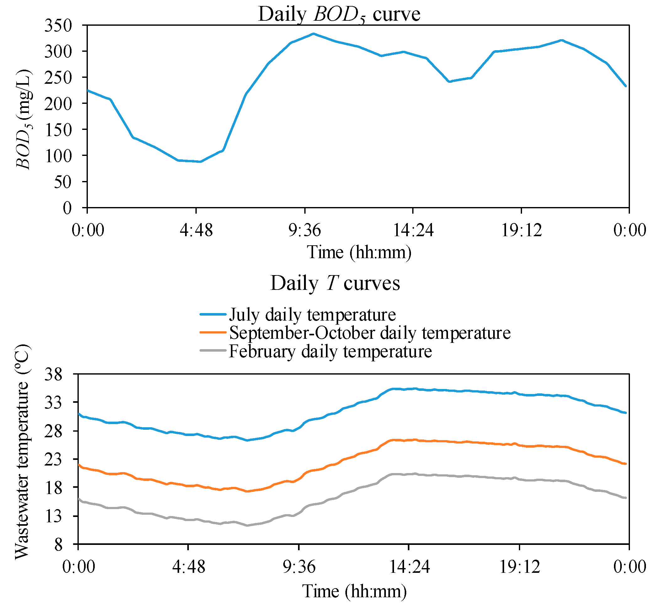Daily BOD₅ and temperature curves of the network were also input data for the code. The calibration process consisted in the variation of parameters M and f_p, where m was set to 0.7. 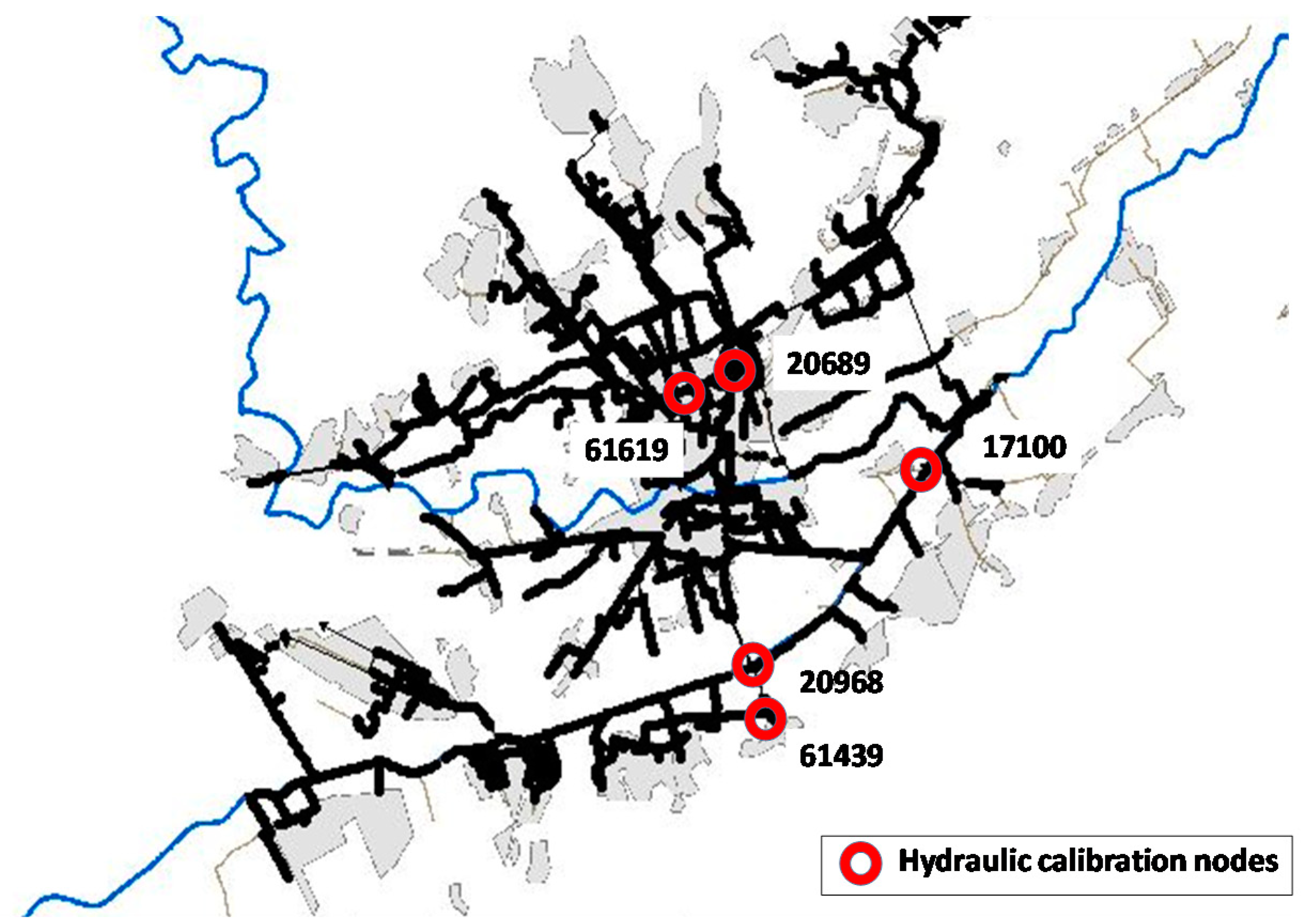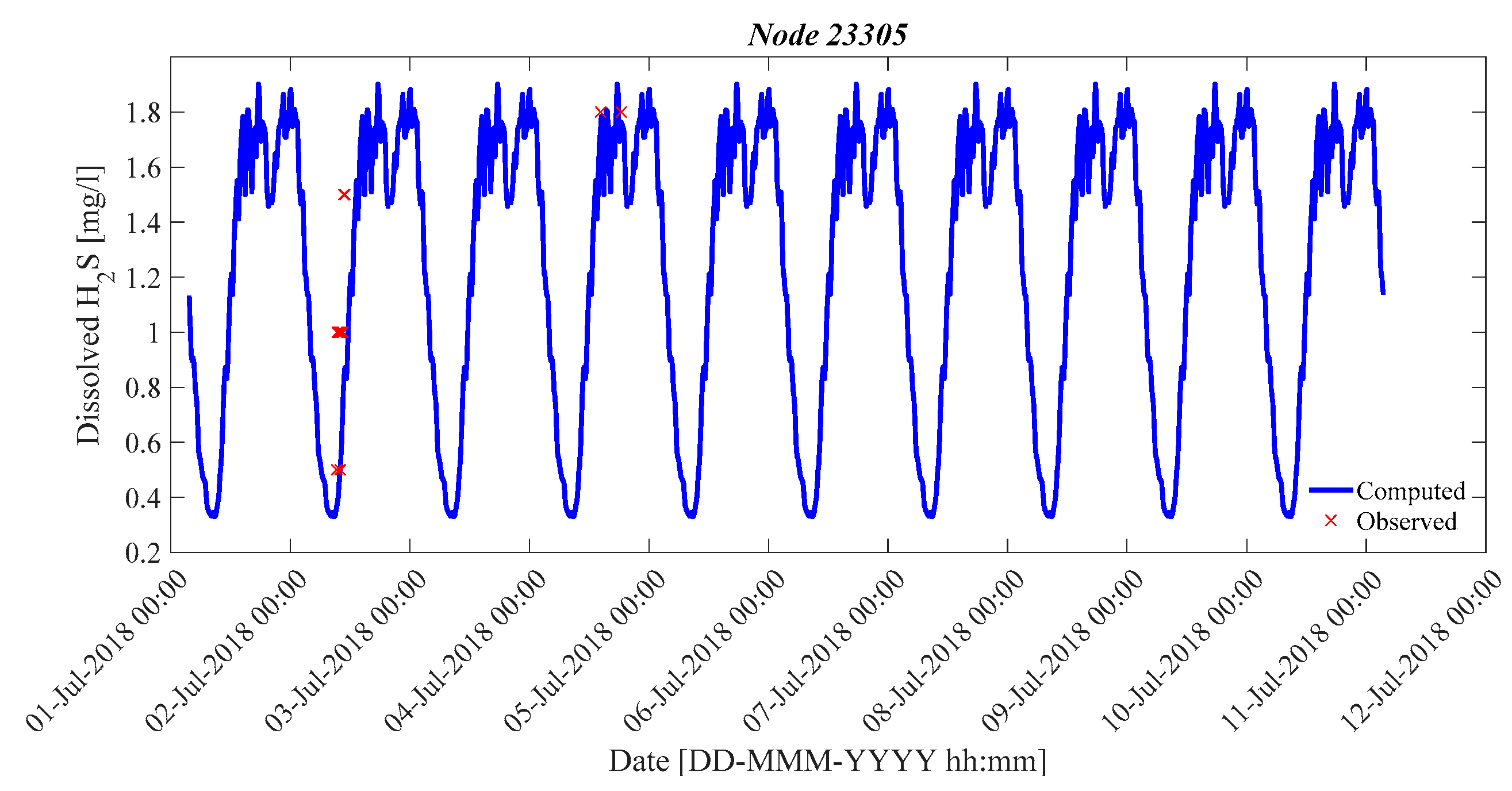Since f_p was in the range from 0.96 to 0.99, the sulfide generation flow coefficient due to the biofilm M was the principal calibration parameter adopting values in the range from 1 to 6 × 10⁻³ with an average value of 3 × 10⁻³. Simulations were undertaken adopting a constant value of the parameters for all the pipes. In the seven calibration nodes and during nine different time periods, acceptable fit to the observed data was achieved with accuracy indexes such as AI and Er in the ranges of 40% and 15%, respectively. This model is considered as the starting point work for the modeling of H₂S in the gas phase inside a sewer network. For future work, it is recommended to increase the amount of observed data to increase the number of calibrated nodes. Furthermore, future work could use different calibration parameters for each of the links, according to different pipeline conditions, such as their age or mechanical wear. Although several previous works in the literature provide the range of the parameters with some approximation and enable simulations to be performed, achieving an accurate model of the network requires a field campaign to measure the calibration parameters.

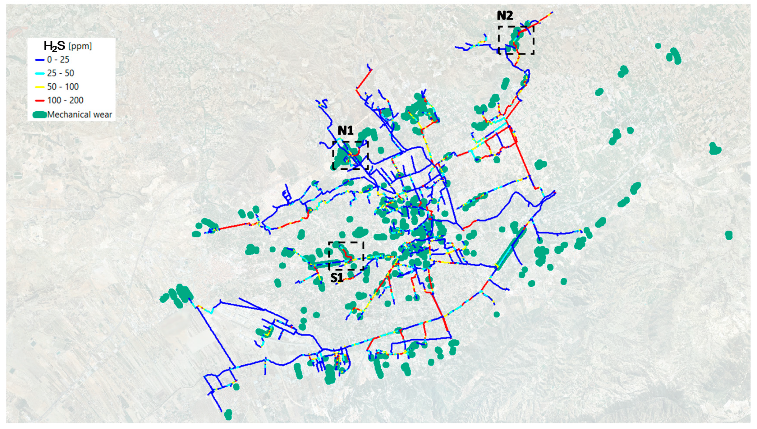
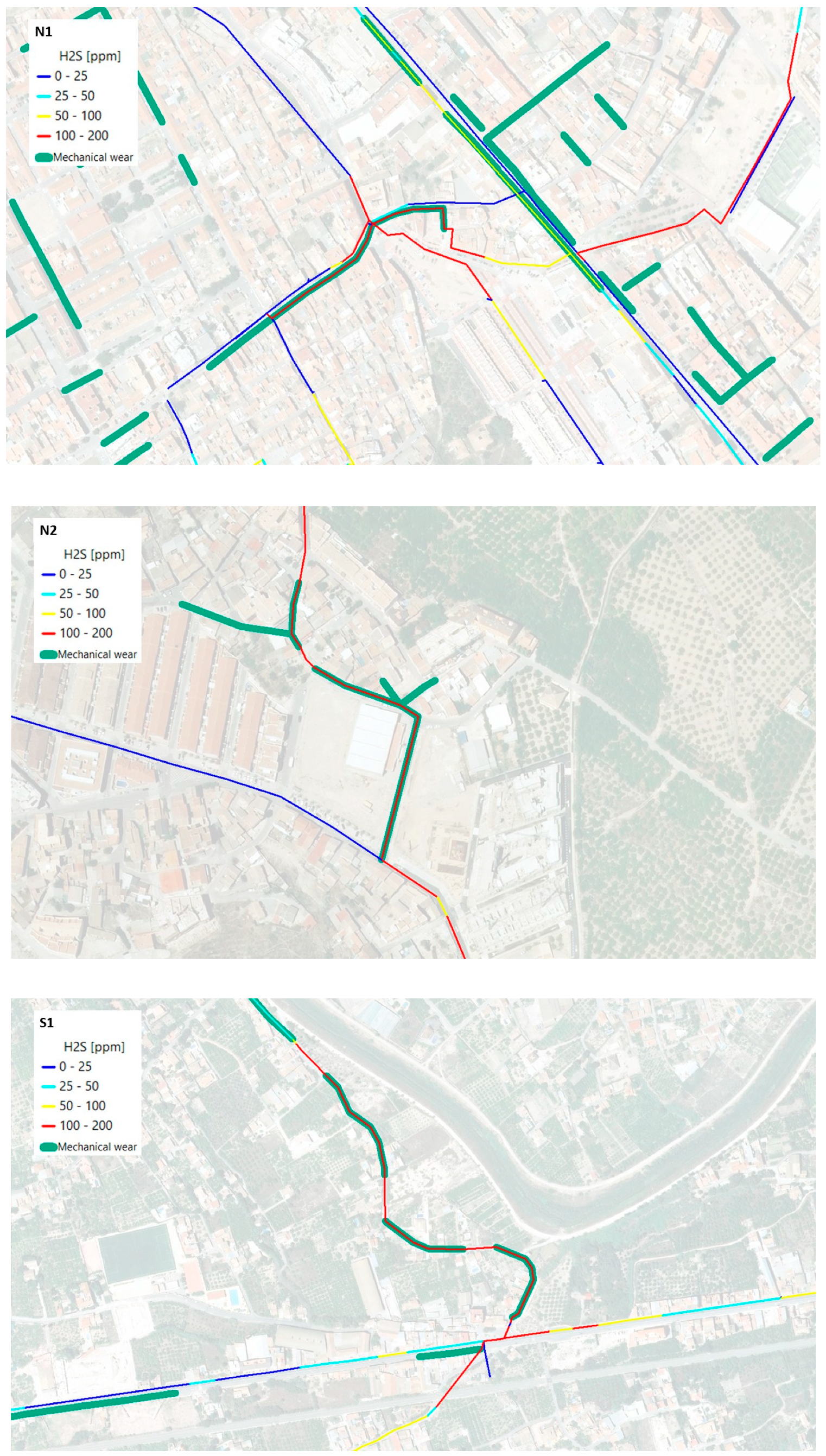
The pipes with the higher values of H₂S—100–200 ppm—are found in areas presenting some of these features:

• Pipes located downstream of a pump station;
• Overloaded pipes where the gas phase represents a low surface;
• Higher values of slope or a combination of these.

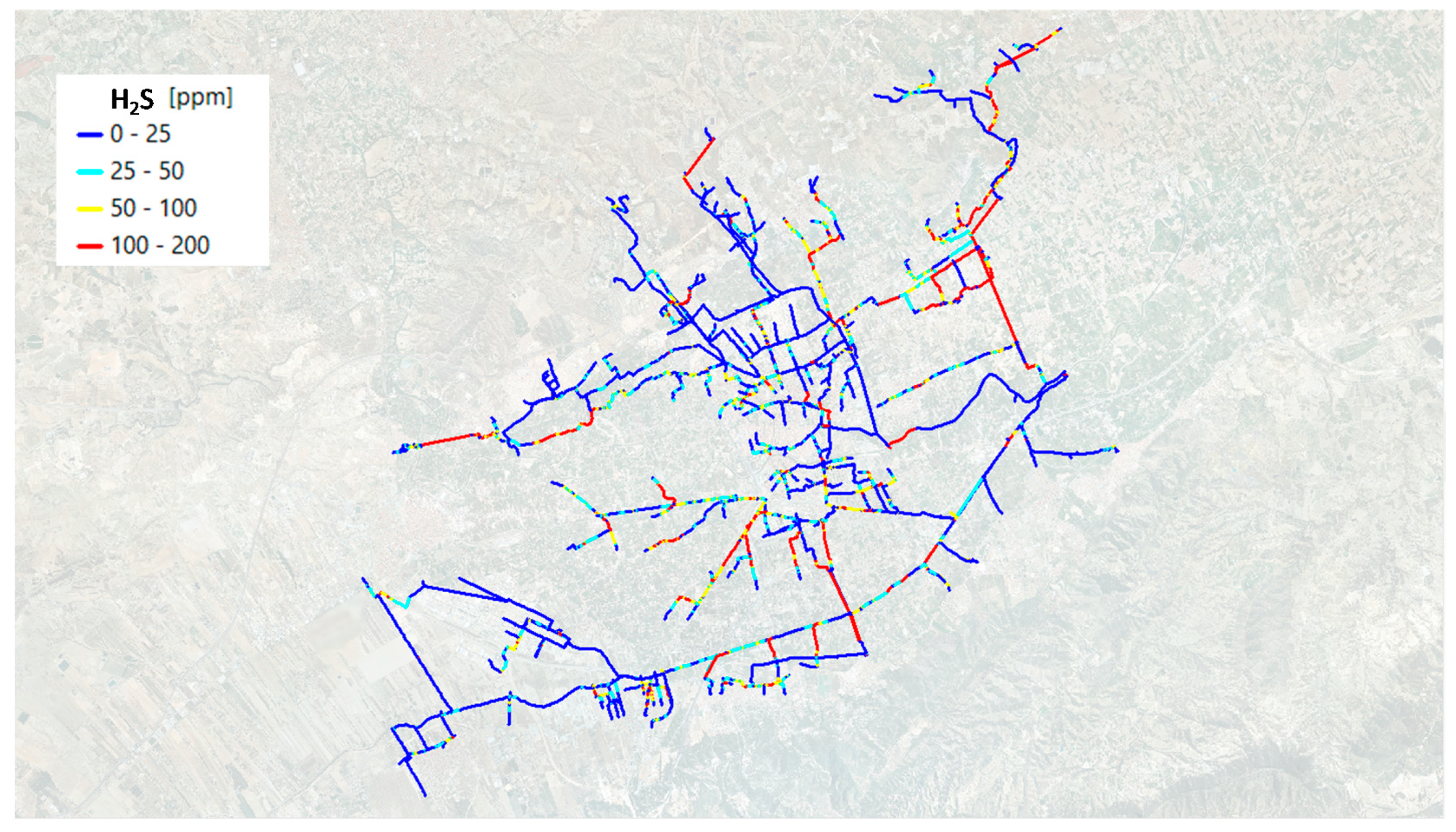
From the simulation results, a map of the annual average H₂S concentration in the gas phase of each pipe was created as a tool that can contribute to asset management. Information on sections with the highest annual average concentrations were obtained, which could be considered in a prioritizing matrix for the decision of the rehabilitation, coating, or renewal of pipes. The calculated annual concentrations were compared with the map of mechanical deterioration of pipes obtained from CCTV. Mechanical deterioration of the pipes has its origin in diverse causes, not only corrosion from H₂S, although sections where high sulfide concentrations coincide with a high degree of mechanical wear could be prioritized for rehabilitation. The sulfide modeling provides valuable information that can be used for better asset management of the sewer network. The H₂S concentration enables the loss of thickness of the wall’s pipes along the time to be calculated, which is a factor to include in any life-cycle analysis of the pipes in conjunction with some other factors [38,39].

References

1. Jiang, G.; Sun, J.; Sharma, K.; Yuan, Z. Corrosion and odor management in sewer systems. Curr. Opin. Biotechnol. 2015, 33, 192–197. [Google Scholar] [CrossRef] [PubMed]
2. Center for Environmental Research Information. Odor and Corrosion Control in Sanitary Sewerage Systems and Treatment Plants: Design Manual; EPA: Washington, DC, USA, 1985.
3. Hvitved-Jacobsen, T.; Vollertsen, J.; Nielsen, A.H. Sewer Processes: Microbial and Chemical Process Engineering of Sewer Networks; CRC Press: Cleveland, OH, USA, 2013. [Google Scholar]
4. García, J.T.; Ruiz-Martínez, D.; Vigueras-Rodríguez, A.; Castillo, L.G.; Carrillo, J.M.; Solano, P.D.; Santos, S.N. Análisis de sensibilidad en la generación de sulfuros en redes de saneamiento. Caso de la ciudad de Murcia. In Proceedings of the Jornadas de Ingeniería del Agua JIA Coruña, Escuela Técnica Superior de Ingenieros de Caminos, A Coruña, Spain, 25–26 October 2017. [Google Scholar]
5. Romanova, A.; Mahmoodian, M.; Alani, A. Influence and interaction of temperature, H2S and pH on concrete sewer pipe corrosion. Int. J. Civ. Environ. Struct. Constr. Archit. Eng. 2014, 8, 621–624. [Google Scholar]
6. Pikaar, I.; Sharma, K.; Hu, S.; Gernjak, W.; Keller, J.; Yuan, Z. Reducing sewer corrosion through integrated urban water management. Science 2014, 345, 812–814. [Google Scholar] [CrossRef]
7. Wells, T.; Melchers, R.E.; Bond, P. Factors involved in the long term corrosion of concrete sewers. In Australasian Corrosion Association Proceedings of Corrosion and Prevention, Coffs Harbour, Australia; Semantic Scholar: Seattle, WA, USA, 2009. [Google Scholar]
8. Koch, G.H.; Brongers, M.P.; Thompson, N.G.; Virmani, Y.P.; Payer, J.H. Corrosion Cost and Preventive Strategies in the United States 2002 (No. FHWA-RD-01-156, R315-01); Federal Highway Administration: Washington, DC, USA, 2002. [Google Scholar]
9. Tscheikner-Gratl, F.; Caradot, N.; Cherqui, F.; Leitão, J.P.; Ahmadi, M.; Langeveld, J.G.; Le Gat, Y.; Scholten, L.; Roghani, B.; Rodríguez, J.P.; et al. Sewer asset management—State of the art and research needs. Urban Water J. 2019, 16, 662–675. [Google Scholar] [CrossRef] [Green Version]
10. Li, B.; Fan, X.; Zhang, J.; Wang, Y.; Chen, F.; Kodagoda, S.; Cunningham, D. Predictive Analytics Toolkit for H2S Estimation and Sewer Corrosion; OZWater: St Leonards, Australia, 2017. [Google Scholar]
11. Caradot, N.; Sonnenberg, H.; Kropp, I.; Ringe, A.; Denhez, S.; Hartmann, A.; Rouault, P. The relevance of sewer deterioration modelling to support asset management strategies. Urban Water J. 2017, 14, 1007–1015. [Google Scholar] [CrossRef]
12. Mahmoodian, M.; Alani, A. Sensitivity analysis for failure assessment of concrete pipes subjected to sulfide corrosion. Urban Water J. 2016, 13, 637–643. [Google Scholar]
13. Sydney, R.; Esfandi, E.; Surapaneni, S. Control concrete sewer corrosion via the crown spray process. Water Environ. Res. 1996, 68, 338–347. [Google Scholar] [CrossRef]
14. García, J.T.; Vigueras-Rodriguez, A.; Castillo, L.G.; Carrillo, J.M. Evaluation of sulfide control by air-injection in sewer force mains: Field and laboratory study. Sustainability 2017, 9, 402. [Google Scholar] [CrossRef] [Green Version]
15. Oviedo, E.R.; Johnson, D.; Shipley, H. Evaluation of hydrogen sulfide concentration and control in a sewer system. Environ. Technol. 2012, 33, 1207–1215. [Google Scholar]
16. Sutherland-Stacey, L.; Corrie, S.; Neethling, A.; Johnson, I.; Gutierrez, O.; Dexter, R.; Yuan, Z.; Keller, J.; Hamilton, G. Continuous measurement of dissolved sulfide in sewer systems. Water Sci. Technol. 2008, 57, 375–381. [Google Scholar] [CrossRef]
17. Liu, Y.; Sharma, K.; Fluggen, M.; O’Halloran, K.; Murthy, S.; Yuan, Z. Online dissolved methane and total dissolved sulfide measurement in sewers. Water Res. 2015, 68, 109–118. [Google Scholar] [CrossRef] [PubMed]
18. Gutierrez, O.; Sudarjanto, G.; Sharma, K.; Keller, J.; Yuan, Z. SCORe-CT: A new method for testing effectiveness of sulfide-control chemicals used in sewer systems. Water Sci. Technol. 2011, 64, 2381–2388. [Google Scholar] [CrossRef] [PubMed]
19. Hvitved-Jacobsen, T.; Vollertsen, J.; Tanaka, N. Wastewater quality changes during transport in sewers—An integrated aerobic and anaerobic model concept for carbon and sulfur microbial transformations. Water Sci. Technol. 1998, 38, 257–264, Printed in errata of 39(2). [Google Scholar] [CrossRef]
20. Vollertsen, J.; Nielsen, A.H.; Jensen, H.S.; Rudelle, E.A.; Hvitved-Jacobsen, T. Modeling the corrosion of concrete sewers. In Proceedings of the 12th International Conference on Urban Drainage, Porto Alegre, Brazil, 11–16 September 2011; pp. 1–8. [Google Scholar]
21. Matos, J.S.; De Sousa, E.R. The forecasting of hydrogen sulfide gas build-up in sewerage collection systems. Water Sci. Technol. 1992, 26, 915–922. [Google Scholar] [CrossRef]
22. Pomeroy, R.D.; Parkhurst, J.D. The forecasting of sulfide build-up rates in sewers. In Proceedings of the Eighth International Conference on Water Pollution Research, Sydney, Australia, 17–22 October 1976; pp. 621–628. [Google Scholar]
23. Boon, A.; Lister, A. Formation of sulfide in rising main sewers and its prevention by injection of oxygen. Prog. Wat. Tech. 1975, 7, 289–300. [Google Scholar]
24. Elmaleh, S.; Delgado, S.; Álvarez, M.; Gómez, L.E.R.; Aguiar, E. Forecasting of HS build-up in a reclaimedwastewater pipe. Water Sci. Technol. 1998, 38, 241–248. [Google Scholar] [CrossRef]
25. Yongsiri, C.; Vollertsen, J.; Hvitved-Jacobsen, T. Hydrogen sulfide emission in sewer networks: A two-phase modeling approach to the sulfur cycle. Water Sci. Technol. 2004, 50, 161–168. [Google Scholar] [CrossRef]
26. Yongsiri, C.; Vollertsen, J.; Hvitved-Jacobsen, T. Air-water transfer of hydrogen sulfide—An approach for application in sewer networks. Proc. Water Environ. Fed. 2002, 2002, 109–122. [Google Scholar] [CrossRef]
27. Lahav, O.; Lu, Y.; Shavit, U.; Loewenthal, R.E. Modeling hydrogen sulfide emission rates in gravity sewage collection systems. J. Environ. Eng. 2004, 130, 1382–1389. [Google Scholar] [CrossRef] [Green Version]
28. Nielsen, A.H.; Vollertsen, J.; Jensen, H.S.; Madsen, H.I.; Hvitved-Jacobsen, T. Aerobic and anaerobic transformations of sulfide in a sewer system—Field study and model simulations. Water Environ. Res. 2008, 80, 16–25. [Google Scholar] [CrossRef]
29. Nielsen, A.H.; Yongsiri, C.; Hvitved-Jacobsen, T.; Vollertsen, J. Simulation of sulfide buildup in wastewater and atmosphere of sewer networks. Water Sci. Technol. 2005, 52, 201–208. [Google Scholar] [CrossRef] [PubMed]
30. Marleni, N.; Park, K.; Lee, T.; Navaratna, D.; Shu, L.; Jegatheesan, V.; Feliciano, A. A methodology for simulating hydrogen sulfide generation in sewer network using EPA SWMM. Desalin. Water Treat. 2015, 54, 1308–1317. [Google Scholar] [CrossRef]
31. Vollertsen, J.; Revilla, N.; Hvitved-Jacobsen, T.; Nielsen, A.H. Modeling sulfides, pH and hydrogen sulfide gas in the sewers of San Francisco. Water Environ. Res. 2015, 87, 1980–1989. [Google Scholar] [CrossRef] [PubMed]
32. Matias, N.; Matos, R.V.; Ferreira, F.; Vollertsen, J.; Matos, J.S. Release of hydrogen sulfide under intermittent flow conditions—The potential of simulation models. Water Sci. Technol. 2017, 77, 777–787. [Google Scholar] [CrossRef] [PubMed]
33. Sharma, K.; de Haas, D.W.; Corrie, S.; O’Halloran, K.; Keller, J.; Yuan, Z. Predicting hydrogen sulfide formation in sewers: A new model. Water 2008, 35, 132–137. [Google Scholar]
34. InfoSewer Pro Suite INNOVIZE®. Available online: https://www.innovyze.com/en-us/products/infosewer (accessed on 25 July 2020).
35. Sun, X.; Jiang, G.; Bond, P.L.; Keller, J. Impact of fluctuations in gaseous H2S concentrations on sulfide uptake by sewer concrete: The effect of high H2S loads. Water Res. 2015, 81, 84–91. [Google Scholar] [CrossRef] [PubMed] [Green Version]
36. Teplý, B.; Rovnaníková, M.; Řoutil, L.; Schejbal, R. Time-variant performance of concrete sewer pipes undergoing biogenic sulfuric acid degradation. J. Pipeline Syst. Eng. Pr. 2018, 9, 04018013. [Google Scholar] [CrossRef]
37. Zamanian, S.; Hur, J.; Shafieezadeh, A. A high-fidelity computational investigation of buried concrete sewer pipes exposed to truckloads and corrosion deterioration. Eng. Struct. 2020, 221, 111043. [Google Scholar] [CrossRef]
38. Mahmoodian, M.; Li, C. Service life prediction of underground concrete pipes subjected to corrosion. In Concrete Solutions; CRC Press: Cleveland, OH, USA, 2011; pp. 551–556. [Google Scholar]
39. Ahammed, M.; Melchers, R.E. Probabilistic analysis of underground pipelines subject to combined stresses and corrosion. Eng. Struct. 1997, 19, 988–994. [Google Scholar] [CrossRef]
40. Rossman, L.A.; Boulos, P.F.; Altman, T. Discrete volume-element method for network water-quality models. J. Water Resour. Plan. Manag. 1993, 119, 505–517. [Google Scholar] [CrossRef] [Green Version]
41. Rossman, L.A.; Clark, R.M.; Grayman, W.M. Modeling chlorine residuals in drinking-water distribution systems. J. Environ. Eng. 1994, 120, 803–820. [Google Scholar] [CrossRef]
42. Rossman, L.A.; Boulos, P.F. Numerical methods for modeling water quality in distribution systems: A comparison. J. Water Resour. Plan. Manag. 1996, 122, 137–146. [Google Scholar] [CrossRef]
43. García, J.T.; Espín-Leal, P.; Vigueras-Rodriguez, A.; Castillo, L.G.; Carrillo, J.M.; Martinez-Solano, P.; Nevado-Santos, S. Urban runoff characteristics in combined sewer overflows (CSOs): Analysis of storm events in southeastern Spain. Water 2017, 9, 303. [Google Scholar] [CrossRef]
44. García, J.T.; Espín-Leal, P.; Vigueras-Rodriguez, A.; Carrillo, J.M.; Castillo, L.G. Synthetic pollutograph by prediction indices: An evaluation in several urban sub-catchments. Sustainability 2018, 10, 2634. [Google Scholar] [CrossRef] [Green Version]
45. Martinez-Solano, P.; Leal, P.E.; Santos, S.N.; Bermejo, J.T.G. Dimensionado de depósitos de retención de contaminación mediante caracterización de las descargas de sistemas unitarios en la ciudad de Murcia. Rev. Recur. Hídricos 2019, 40, 55–64. [Google Scholar] [CrossRef]
46. Pomeroy, R. Generation and control of sulfide in filled pipes. Sew. Ind. Wastes 1959, 31, 1082–1095. [Google Scholar]
47. Pomeroy, R.D.; Parkhurst, J.D. Forecasting of sulfide buildup rates in sewers. Prog. Water Technol. 1977, 9, 621–628. [Google Scholar]
48. U.S. EPA. Process Design Manual for Sulfide Control and in Sanitary Sewerage Systems; USEPA: Washington, DC, USA, 1974.
49. Moriasi, D.N.; Arnold, J.G.; Van Liew, M.W.; Bingner, R.L.; Harmel, R.D.; Veith, T.L. Model evaluation guidelines for systematic quantification of accuracy in watershed simulations. Trans. ASABE 2007, 50, 885–900. [Google Scholar] [CrossRef]
50. Krause, P.; Boyle, D.P.; Bäse, F. Comparison of different efficiency criteria for hydrological model assessment. Adv. Geosci. 2005, 5, 89–97. [Google Scholar] [CrossRef] [Green Version]
51. García, J.T.; Harrington, J.R. Fine sediment modeling during storm-based events in the River Bandon, Ireland. Water 2019, 11, 1523. [Google Scholar] [CrossRef] [Green Version]
Figure 1. (a) View of the degradation of a sewer in Corredera Street in the town of Javalí Nuevo (Murcia, Spain). (b) Detail of degraded pipe because of the action of hydrogen sulfide (H2S) proposed in Odor and Corrosion Control in Sanitary Sewerage Systems and Treatment Plants: Design Manual [2].
Sustainability 12 07643 g001
Figure 2. View of part of the map of the pipelines with mechanical deterioration observed with CCTV inspection in the city of Murcia by Municipal Sanitation Utility of Murcia (EMUASA).
Sustainability 12 07643 g002
Figure 3. View of the hydraulic model of the main sewers of the city of Murcia in the Storm Water Management Model (SWMM) where some of the calibration nodes are indicated.
Sustainability 12 07643 g003
Figure 4. Daily curve of temperature and biochemical oxygen demand (BOD5) of the wastewater that circulates through the network in dry weather.
Sustainability 12 07643 g004
Figure 5. Location of sulfide calibration nodes in the main sewer network of the city of Murcia.
Sustainability 12 07643 g005
Figure 6. Simulated and observed values of H2S in the gas phase of the sewers in the calibration nodes in different time periods.
Sustainability 12 07643 g006
Figure 7. Sensitivity of the H2S concentration in the gas phase of node 23,309.
Sustainability 12 07643 g007
Figure 8. Simulated and observed values of dissolved H2S in the wastewater of the sewers at node 27,291. The calculated values are shown by a continuous blue line, whilst the measured samples are represented with red crosses.
Sustainability 12 07643 g008aSustainability 12 07643 g008b
Figure 9. Annual average sulfide concentrations at pipe scale of the main sewer network of the city of Murcia.
Sustainability 12 07643 g009
Figure 10. General view of the comparison of mechanical deterioration observed with CCTV inspection and average sulfide concentration where the investigated zones are marked.
Sustainability 12 07643 g010
Figure 11. Comparison of mechanical deterioration observed with CCTV inspection and average sulfide concentration at the area marked as S1 in Figure 10.
Sustainability 12 07643 g011