The Utilization of Normalized Difference Vegetation Index to Map Habitat Quality in Turin (Italy)

Abstract

The integration of ecosystem service mapping in decision-making is crucial to place effective urban design and sustainable planning solutions. Nonetheless, often ecosystem service maps are the product of different data inputs that influences the final modeling output thus affecting final decisions, especially when a finer and site-specific assessment is required to design practical and effective solutions. In this work, the city of Turin (Northwest Italy) was selected as a test site for an empirical experiment of ecosystem service mapping using the software Integrated Valuation of Ecosystem Services and Tradeoffs (InVEST): two habitat quality models of the city were compared in a Geographic Information System environment, the first using the “traditional” sensitivity employed during the LIFE SAM4CP European research while the second using the natural difference vegetation index to re-assign the sensitivity scores. Results demonstrate that the integration of site-specific information in the habitat quality input model generates a different result, which is capable of differentiating all those dense built-up areas of the dense settlement system that provide ecosystem supporting functions at the city-level. These differences were analyzed to define new green hotspots in the compact city while furnishing a new perspective for sustainable city planning.

1. Introduction

Urban green infrastructure (UGI) aims to develop green networks on limited space in compact cities [1]. UGIs are mainly designed to provide multifunctional spaces [2,3], whereas multifunctionality is here intended as the ability of green spaces to provide multiple benefits concurrently [2,4,5]. The basic meaning of multifunctionality is that UGI—and more broadly, urban green spaces—offers a variety of functions, for example, ecological, social, and economic ones [6,7,8]. Multifunctionality is also described as the capacity of green spaces to provide multiple ecosystem services (ESs) [2,9,10,11].

Combining different functions to maximize the ecological benefits in limited spaces is particularly important in dense urban areas, where greenery is scarce, and even more in compact cities [12]. This view is crucial since the effectiveness of ESs provision increases when they are located close to the demand areas and, therefore, where the city is compact and densely populated [13,14]. Urban areas are the ones where the ESs supply meets at its maximum the demand for green and healthier spaces [15].

On this ground, significant challenges remain in assessing and valuing individual urban ESs, especially those that represent supporting ones [16,17], as well as in understanding the spatial distribution, tradeoffs, and synergies of multiple services at the citywide scale [18,19]. In this view, one of the most relevant supporting ecosystem services in urban areas is the ecological integrity of green spaces [20,21,22].

There is a huge amount of bibliography that employed many land-use-driven indexes to determine the environmental quality of urban areas, especially to differentiate the different ecological values in the dense settlement and the surrounding open fields. As it has been originally pointed out by McHargh [23], the ecological approach to urban systems evaluates the “integrity” of places based on a coupled integration of different biophysical factors that are mainly addressed by employing land-use classification and its interaction with different sources of threats [24].

Indexes of biodiversity range from the biological territorial capacity, which has been used to set the minimum environmental quality of land-use transformations, to the ecological quality, which is considered one of the most relevant supporting ecosystem services for the natural capital [25,26,27].

These indexes are the output of statistical procedures that uses benefit-transfer methods, while the need for site-specific baseline data derived from mapping ESs (using software such as Integrated Valuation of Ecosystem Services and Tradeoffs—InVEST) increased during recent years while requiring in-depth input data and site-specific knowledge of the local situation.

Among different methodological assessments, mapping the habitat quality (HQ) of urban systems has become pivotal for environmental analysis especially in all those dense urban areas where green spaces are considered essential for many ESs and the well-being of citizens [2,21,28].

Nevertheless, while in theory, the capacity of urban green areas to provide multiple benefits is well-recognized, the qualitative distinction on urban green spaces in compact cities is more generally determined by their social accessibility, their extension, or their land-use composition and less by their intrinsic biophysical properties [24,29,30].

Urban Ecosystem Services

Urban systems are characterized by high spatial heterogeneity that complicates environmental analysis and requires data at an excellent spatial and spectral resolution, which is often unavailable or time-consuming and expensive to obtain [31,32]. To overcome the issue, a new kind of data is highly needed to support the design of UGI, shortening the long-time processing that affects ESs mapping and providing consistent and updated data to aid the definition of effective environmental policies in urban areas [33,34].

From a general and theoretical point of view, the environmental quality of green urban areas is generally considered low, since fragmentation has been found to be the most threatening cause of ecological degradation [35]. This is true to a certain extent since this approach is undoubtedly valid at the higher-landscape level. However, if it is assumed that green urban areas are fragmented for their objective condition (urban green areas are located in the core of the built-up settlement system), and besides that, an irreversible “anthropic” character weakens the original ecological integrity, the need to adopt a differential biophysical distinction becomes crucial to prioritize areas of intervention and the kind of specific solution that is required to develop healthier urban transformations while greening the city [31,36]. Here, “differential” is referred to as the internal distinction to classify the urban green elements with different degrees of thematic accuracy [37], which is opposed to the macroscopic “absolute” distinction between the low-value urban green and the high-value rural or natural environment [35].

On this premise, a detailed quantitative biophysical assessment should be developed, delivering fine-grained results and capturing the broad range of values relevant for planning aiding urban design solutions during the decision-making phases supported by ES maps [11].

Recently, the Piedmont Region (Northwest Italy) introduced the first normalized difference vegetation index (NDVI) as a resource that helps to monitor the state of the environment. The index synthesizes the presence/health of vegetation and its consistency in all the regions. This information is crucial to set how urban and sub-urban areas differ in their vegetation density and quality, giving a quick and easy-to-understand representation of the green “health” both in the densely built environment and the open agricultural fields [38,39].

In this paper, the NDVI was employed to define the sensitivity of the land-use/land-cover (LULC) table to the HQ model (InVEST), looking at how the output performs when used for urban design purposes (e.g., UGI design) [40].

The question that this paper tries to answer is how the integration of a quantitative index such as the NDVI can capture the internal difference of urban green elements while helping in defining the HQ input sensitivity table and providing better ES modeling outputs. Notably, within this research, the table for the sensitivity of each LULC type to threats was revised according to an analytical assessment of the NDVI.

In terms of utilization, the NDVI represents the state of the environment since it is the product of an infrared digital image that can be downloaded from Copernicus Services [41] while habitat quality is the product of an ecosystem service modeling output that mixes two sources of input [9]: the land use with a specific sensitivity score and the source of threats with a defined distance of disturbance.

The NDVI is derived by hourly released sat-images, freely downloadable and objective in their description of the ecological integrity. With near-infrared detectors, remotely sensed images can measure the intensity of light coming off the Earth in visible and near-infrared wavelengths and quantify the photosynthetic capacity of the vegetation in a given unit of space. In general, a high near-infrared wavelength represents dense vegetation that contains forests. On the other hand, less intensity of near-infrared wavelengths reflected may mean grassland, tundra, or desert. NDVI results are being increasingly used to monitor the forest dynamics or to check the seasonal growth of plants or crops to maximize the production. At the urban scale, the NDVI detects small green objects (green roof, vertical green, little plants, riparian vegetation, street planting systems, etc.) while furnishing optimal support in those urban design tools that aims at modifying the urban systems by micro-transformations in dense built-up space (e.g., brownfield redevelopment).

It is well-known that sat-images are sensitive to seasonal changes in the land uses, but this kind of problem also affects the digitalization process employed for a LULC dataset, which is the crucial input variable of habitat quality. Therefore, the research conducted here took the available information (input data) of HQ modeled during the Life SAM4CP research and compared the standard values with a new modeling output that is based on the utilization of the NDVI as a new proxy of sensitivity [42,43,44]. Both HQ models were produced using the latest version of InVEST (suite of models produced by the Natural Capital Project, Stanford University, Stanford, California v. 3.7.0) sharing the same catchment area of Turin to see how the two outputs differ in each zone of the city.

Maps were statistically and visually compared to detect significant synergies and differences to see which modeling output best reflects the urban “differential” character of the environment and how the systematic utilization of the result should better support the definition of UGI.

In section two, the methodology of assessment is defined with a detailed explanation of data sources and HQ modeling, while in part three, the discussion focuses on the data interpretation and the comparison between the baseline HQ and the new NDVI-based HQ. Results sum up the relevant information derived from this empirical test, displaying that the NDVI is a quite useful input for ES modeling, especially in urban areas where the vegetation canopy influences the environmental performance of the dense built-up system, revealing that traditional modeling analysis that associates site-specific indexes to land uses fails to address the diversity of specific sites. In the conclusions, this method is used to extract the high HQ areas that support the land-use regulation at the local scale, providing an example of UGI structure in the city of Turin [45].

2. Materials and Methods

2.1. The Context of the Study

The city of Turin is located in the northwest of Italy and is among the most populated municipalities of the country (it is the fourth-biggest city according to the national census of 2011, see Figure 1). It counts around 882,000 citizens distributed in an administrative area that spans about 130 km² [46].

The city is placed at 240 m above the sea level since it has been developed at the foot of the Western Alps, while in the east and south, the city is bordered by hilly landscapes of Turin and Monferrato. The orography of the town is conditioned by the fluvial evolution of the Po River and its tributaries (mainly the Sangone, Dora, and Stura that cross the city).

The settlement system is densely constructed with compact urban development and a high degree of impermeable areas. According to the Digital Topographic Geodatabase of 2018, more than 7400 hectares of the city are sealed, with an average sealing rate that equals to 57.55% (calculated as the fraction of sealed surface on the total administrative area).

From an ecological perspective, the city is surrounded by high-quality peri-urban green areas as demonstrated by the “Corona Verde” project [47] where fluvial corridors along the main water streams define the structural connection between the green backbone of the Po River, including the eastern hill, and the western part of the city that is connected by radial green axes along with fluvial areas (Dora and Stura Rivers, see Figure 2).

2.2. Data

2.2.1. The Normalized Difference Vegetation Index

The normalized difference vegetation index detects the consistency of vegetation by measuring the difference between near-infrared (which is reflected by vegetation) and red light (which is absorbed by the plant) [48].

Healthy vegetation reflects more near-infrared (NIR) and green light compared to other wavelengths. However, it absorbs more red and blue light. The index values range from −1 (highly likely to be water that entirely reflects solar radiation) to +1 (highly likely to be dense green leaves that absorb solar radiation) and cover all kinds of land uses (this means that the green roofs and small vegetated areas in the urban compact built-up system are well-recognized by this index).

When the indicator tends to zero, the possibility is that it represents settlements.

In the end, the NDVI measures the quality of vegetation. Compared with the traditional soil sealing/high-resolution imperviousness layer that measures the quantity of soil covered or uncovered by impermeable surface, the NDVI contains another type of information that represents well the quality, instead of the quantity, of the permeable land. Therefore, this kind of information in the dense urban catchment helps in understanding the quality of urban green lots, even those of low and small size, achieving an increased comprehension of the overall environmental conditions of urban areas, which reflect both the presence and the quality of the permeable space in urban areas.

The NDVI employed in this research was provided by the Regional Agency for Environmental Protection in Piedmont (ARPA Piemonte) and obtained by Sentinel 2A image of 2016 (Copernicus Program). Images were mosaicked by three bands that correspond to monitor canals of spring, summer, and autumn 2016. For the purpose of this research, Band-2 (June 2016) was selected since it was cloud-free at 100%, then the raster was ranked with values from 0 to 1 indicating low to high green quality (Figure 3).

2.2.2. Habitat Quality Model

The HQ model expresses the ability of the ecosystem to provide appropriate conditions for individual and population persistence. The index is calculated using InVEST, which is a freely accessible and downloadable suite of tools to map and assess the ES provision for different types of services. The HQ final output reflects both the proximity of the habitat to anthropic land uses and the threats caused by anthropic areas. The model can be employed to allow the user to obtain a map of suitable habitat for certain fauna, or it can be employed more generally, while getting a general assessment of the quality of habitats for all species. In the latter case, HQ is considered a synthetic indicator thus representing a proxy of the quality of the landscape.

The HQ model requires (i) inputs on the LULC map, (ii) threats to habitats articulated in the maximum distance over which each threat affects each habitat, and (iii) the habitat type and sensitivity of each habitat type to the threats.

The last value (habitat type) is fundamental since it assigns to each LULC a specific value to habitats, ranging from 0 to 1, that is normally defined by bibliographic research and not by empirical research or an expert’s judgment. Nonetheless, often scoring sensitivity is crucial to the modeling results, and this assignment is (i) generally adapted from original bibliographic parametric sources and (ii) often de-contextualized, while the map of HQ represents a relative value that should be site-specifically designed.

Therefore, the habitat index input variable is essential since the model works by assigning an initial value to each land cover. Then it defines the interaction of the habitat with the threats by generating a degradation trend of each habitat type with linear or exponential decaying functions.

What we tested in this work was how the HQ model differs while using a “traditional sensitivity table” (the one employed during the SAM4CP research activities) and a new “NDVI-driven” sensitivity table which was revised using the average value of the NDVI index calculated in the land-use/land-cover input. The “traditional” sensitivity input table was set with a “typical” bibliographic parametric approach and then adjusted by an expert-based evaluation supported by the SAM4CP research partner of ISPRA (the National Superior Institute for Environmental Research and Protection), while the second sensitivity table was remote-sensing-derived (scores were assigned calculating the mean NDVI value for each LULC). Therefore, the two methodologies differ in substantial terms since the first is the product of a qualitative evaluation while the second is the product of quantitative measurement. For this reason, the two outputs are not properly “comparable”, and thus our intention is limited to check which of the two best aid the decision-making phase of defining a hypothetical UGI.

We are well-aware of the fact that the NDVI is an index that holds certain limits in representing the ecological integrity of urban areas; nonetheless, our scope is not to demonstrate which is the “best” sensitivity input table but to find a stepwise approach to increase the quality of ecosystem mapping. In addition, our scope is to empirically demonstrate if the introduction of quantitative remotely sensed data in the input produces a tangible effect of HQ values in the dense urban areas of Turin while contributing to the design of urban green infrastructure.

2.3. Procedure

As introduced, the procedure hereafter presented served to re-define the input parameter of habitat in the input “Sensitivity table”. The analysis was conducted using Esri ArcGIS v. 10.6 (Environmental Systems Research Institute, Redlands, California) for GIS data while employing Microsoft Excel to determine the final average values of habitat for each LULC class.

Firstly, the NDVI and the LULC raster of the Piedmont Region were pre-processed by clipping the borders in the administrative area of Torino and its surrounding municipalities to obtain a new HQ model that does not contain the edging effect [27]. Edging refers to the possible interference that is generated in the perimeters of raster inputs, where the multiple interactions between threats and sensitivities are affected by the limits of the geometrical features.

Secondly, each raster file was vectorized using the “raster to polygon” function. Then, the two datasets were intersected while obtaining a new shapefile where each LULC category was associated with an NDVI value.

Finally, MS Excel was used to set the final average NDVI value for each LULC category. For this operation, the following procedure was applied. The new intersected shapefile (NDVI with LULC) was statistically evaluated through the utilization of the .dbf file. A Microsoft Office pivot table was settled linking each row (LULC code) with the average value of the NDVI. The new value was evaluated against the original one (see

Table 1. Comparison between SAM4CP and NDVI-driven sensitivity values. LULC: land-use/land-cover.

LULC	LULC Desc	SAM4CP Habitat Values	NDVI-Driven Habitat Values
Macro-category 1	Urban Areas	0.09	0.48
Macro-category 2	Agricultural Land	0.42	0.66
Macro-category 3	Natural and Seminatural	0.85	0.75
Macro-category 4	Humid areas	1.00	0.91
Macro-category 5	Water	0.74	0.40

) to have a direct representation of the major discrepancies between the two inputs.

In Table 1 the two values of sensitivity are compared. For easier comprehension, the original values of sensitivity were titled “SAM4CP habitat values” while the new results “NDVI-driven habitat values”.

On average, the sensitivity values in the two columns differ by 152.5% with a marked distinction in urban areas, where the NDVI sensitivity values are slightly higher than the SAM4CP values. The difference is less evident in the macro-category of agricultural land (NDVI values are averagely higher by 69.81% than SAM4CP values) while it is less relevant in the natural and seminatural areas (in that case NDVI values are, on average, lower by 10.13% than SAM4CP values).

It has to be declared that Macro-category 5 of LULC (water) is affected by the NDVI detection since the index tends to be equal to 0 where the reflectance of water streams is detected (therefore the average negative difference between the NDVI and SAM4CP of 8.35% should be evaluated bearing this limit in mind). As it is well-known, water streams provide ESs. Nonetheless, for this scope, this limitation is negligible since (i) we aim to evaluate the quality of soil ESs leaving apart considerations regarding watercourses and water streams and (ii) the employed dataset has a fine resolution, and thus the detection of the canopy of trees bordering the streams reduces this limit.

Once the new NDVI-driven values were assigned to each LULC category, the new HQ model was launched using the common .csv input threats data (see

Table 2. Table of threats.

THREAT	MAX_DIST	WEIGHT	DECAY
1111	1.70	0.80	linear
1113	1.70	0.80	linear
1121	1.70	0.80	linear
1123	1.70	0.80	linear
1211	1.70	0.80	linear
1213	1.70	0.80	linear
1221	1.60	0.90	linear
1222	1.60	0.60	linear
1223	1.70	0.80	linear
1240	1.70	0.80	linear
1300	1.70	0.80	linear
1310	1.70	0.80	linear
1321	1.70	0.80	linear
1332	1.70	0.80	linear
1422	1.70	0.80	linear

).

The model produced two results: SAM4CP and NDVI-driven that were analyzed and processed, considering the limitations mentioned above.

3. Results

The two HQ maps were preliminary observed and visually compared (see Figure 4). Outputs were displayed using 1-Band pseudo-colors (green-to-red) indicating a good (green) or bad (red) performance of the HQ indicator. Both raster outputs were generated with the same pixel resolution (columns and rows: 3093, 2960; number of bands: 1; cell size: 5 × 5 m; format: grid).

The left image represents the SAM4CP raster output, while the right image is the NDVI-driven HQ output. At a first look, between the two maps, it is quite visible the shifting of intense red colors to a lighter rose (representing a diffused higher quality in the urban catchment) tone while reaching a flattened and less-contrasted distribution of HQ in the urban area in the NDVI output. While, in the left image, the contrast is more visible (dark and contrasted), the right image appears to be less contrasted (light and diffused) because the NDVI-driven “sensitivity” table inputted higher habitat values to all densely-built urbanized areas.

As earlier introduced, it is quite visible the difference in water streams, where the dark green of the SAM4CP model becomes light green in the NDVI-driven output. Nonetheless, this result is the product of the limitation mentioned above.

At a first look, it seems that relevant differences are present in the densely built-up area, which is divided into two primary tonalities of red in the SAM4CP output while in mashed in a lighter mixed-up rose-to-red tonality in the NDVI-driven output. Dark green areas remain the same while decreasing their “darkness” in the hill and the city river streams in the NDVI-driven output. Therefore, the “visible” result indicates the NDVI-driven output as less capable of making a marked distinction between higher and lower HQ clusters in the urban environment.

However, this first-look judgment is only partial and limited to a first assessment. To test this heuristic result, the statistical distribution of the two outputs was calculated, discovering the differences between the two outputs. First, the two rasters were vectorized by the raster-to-polygon function, and then statistical analysis was employed to compare the data; the results are summarized in

Table 3. Statistics table of the output features between SAM4CP and NDVI-driven habitat quality.

	SAM4CP HQ Output	NDVI HQ Output
Min	0.00	0.46
Max	1.00	0.83
Mean	0.12	0.55
Standard Deviation	0.17	0.04

Then a clustering analysis was performed, and finally, a visualization of the distribution of values was commented on.

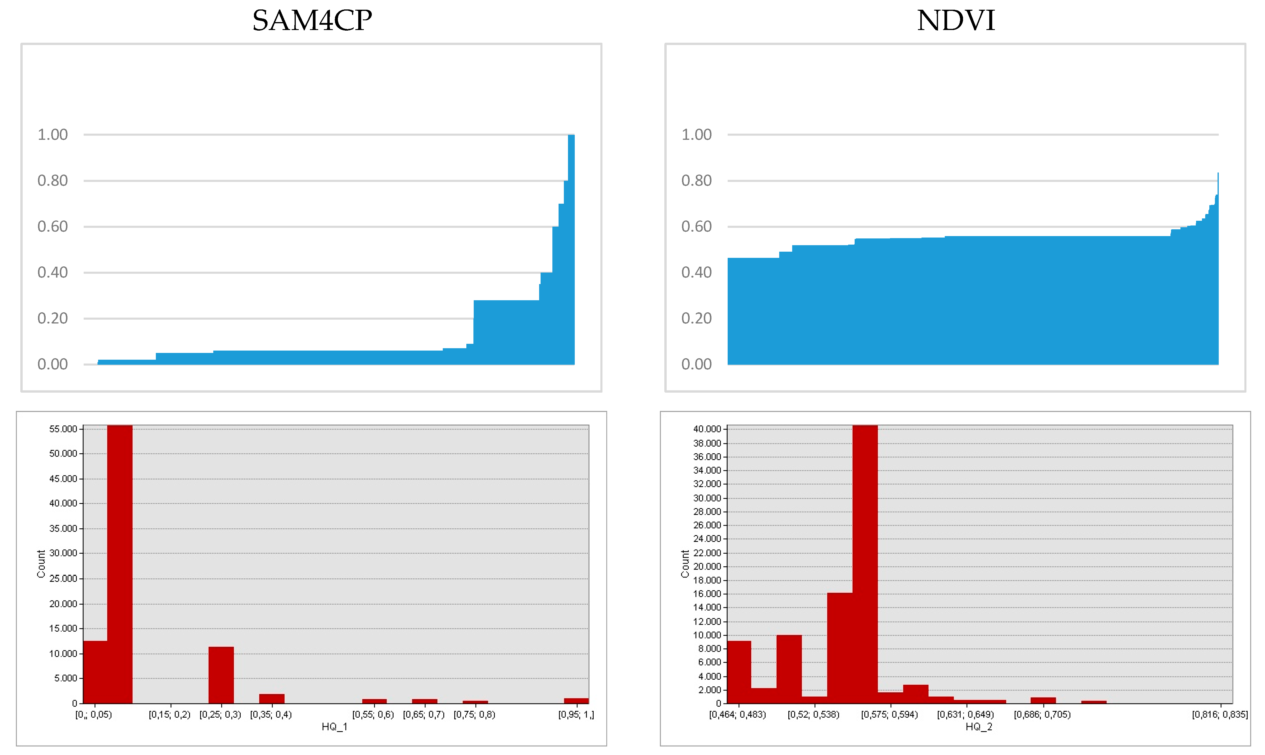
Table 3 shows the statistic of outputs: while the SAM4CP HQ generates values ranging from 0 to 1, the NDVI HQ output ranges from 0.46 to 0.83, narrowing the “extremes” of the original variance between the observed values. Nevertheless, the mean of NDVI HQ is much higher (0.55) than the mean of SAM4CP (0.12), indicating that the two results differ significantly.

Statistics confirm the “visual” judgment, reflecting the more “dark and contrasted” (higher standard deviation) vs. “light and diffused” interpretation of the pseudo-color image (Figure 3).

Nonetheless, to deepen the interpretation of results, the clustering analysis using the spatial analysis statistics tools (high/low clustering) was applied, discovering the following: given the z-score of 63.1, the SAM4CP habitat values present a high-clustered pattern while, on the contrary, given the z-score of -44.3 the NDVI-driven habitat value presents a low-clustered pattern. Therefore, even the clustering analysis confirms the NDVI output as less capable of providing a marked distinction between high/low values in the catchment. However, the main question of what kinds of differences there are between the two outputs remains unanswered and, to answer this question, a distribution and frequencies of HQ values between the outputs were analyzed (see Figure 5).

The graph represented in Figure 5 displays that the values have a significantly different distribution. At first, even if it is true that the general variance of values is higher in the SAM4CP output (y values are distributed approximating an exponential curve with a few extreme values in the SAM4CP while the distribution of NDVI is “flattened” with a “peak” when y > 0.55), the frequencies demonstrate that the SAM4CP output variance is mainly conditioned by the strong polarization around 0.05 to 0.10 class (with a frequency above the 55,000 features), while the NDVI output frequencies are less polarized reaching one peak around 0.55 to 0.56 (of 40,000 features) and then presenting at least three other peaks between 0.46 and 0.55 values.

To simplify the concept, the “dark and contrasted” configuration of the SAM4CP output is affected by a high concentration of low values on the built-up environment with a few outliers in the frequencies, while the NDVI output displays an averagely highly-scattered pattern with at least four peaks between 0.4 and 0.6 HQ values. Statistically, the NDVI output appears to be more reliable since it is capable of classifying the internal differentiation of HQ urban values, while, on the other hand, SAM4CP output is more suitable to indicate the “absolute” differentiation of urban land (low HQ) vs. rural land (high HQ).

Indeed, even if the difference between “red” and “green” (Figure 4) areas is less visible in the NDVI output, there is a wider “internal” distribution of features around higher values in the urban area, revealing the possibility to better classify and distinguish the HQ values of the dense settlements. On the other hand, SAM4CP displays more contrast, but it is highly conditioned by a few high/low clusters.

This happens because the NDVI-driven “sensitivity” values capture the heterogeneity of internal built-up dense vegetated areas. The dense built-up zones of the city of Turin are porous, with large private spaces of trees and brushes and well-planted parks. Furthermore, road axes in Turin have permeable planted spaces with certain central areas dedicated to green pedestrian corridors and boulevards designed with the ancient road-design approach of the 19th century. All these elements are somehow “detected” by the NDVI thus influencing the new HQ output.

Figure 6 helps in understanding where the two results greatly differ. The two maps were superimposed with a spatial intersection, then the difference between each feature value was colored from dark blue (NDVI values are far less than SAM4CP values) to red (NDVI values are far more than SAM4CP values).

As already mentioned, the dense urban settlement of the city displays a higher mean value in the NDVI output, with a few urban features where the NDVI is far higher than the SAM4CP: the monumental cemetery (that is an urban feature that hosts biodiversity with a large unpaved area and a good tree density) and the dumpsite and the adjacent “Basse di Stura” which are two places representing typical ex-industrial sites that during the last twenty years experienced a process of re-naturalization while achieving a better environmental quality than in the past. However, the NDVI output has a far lower value in the hill and in the peri-urban agricultural land where the diffuse urbanization lowers the environmental quality of open spaces.

In the end, while flattening the extremely low/high values, the NDVI distribution captures the broad range of differences that exists at the city-scale, offering an interesting modeling output.

4. Discussion

To support the empirical argumentation of results, a further analytical step was applied to simplify the NDVI modeling output and achieve an easy-to-understand map where those areas of the city that display good HQ values emerge to be well-identified. This final analytical step was made to aid the analytical discussion around the utilization of HQ models to support the decision-making process in urban planning.

Therefore, the NDVI HQ map was post-processed with a hotspot analysis, obtaining a grouped distribution of values around intervals of “significance” or “non-significance” [4,49,50]. Hot spots and cold spots are clusters of statistically relevant values that represent spatially auto-correlated clusters (red and blue) or areas of no relevance (white).

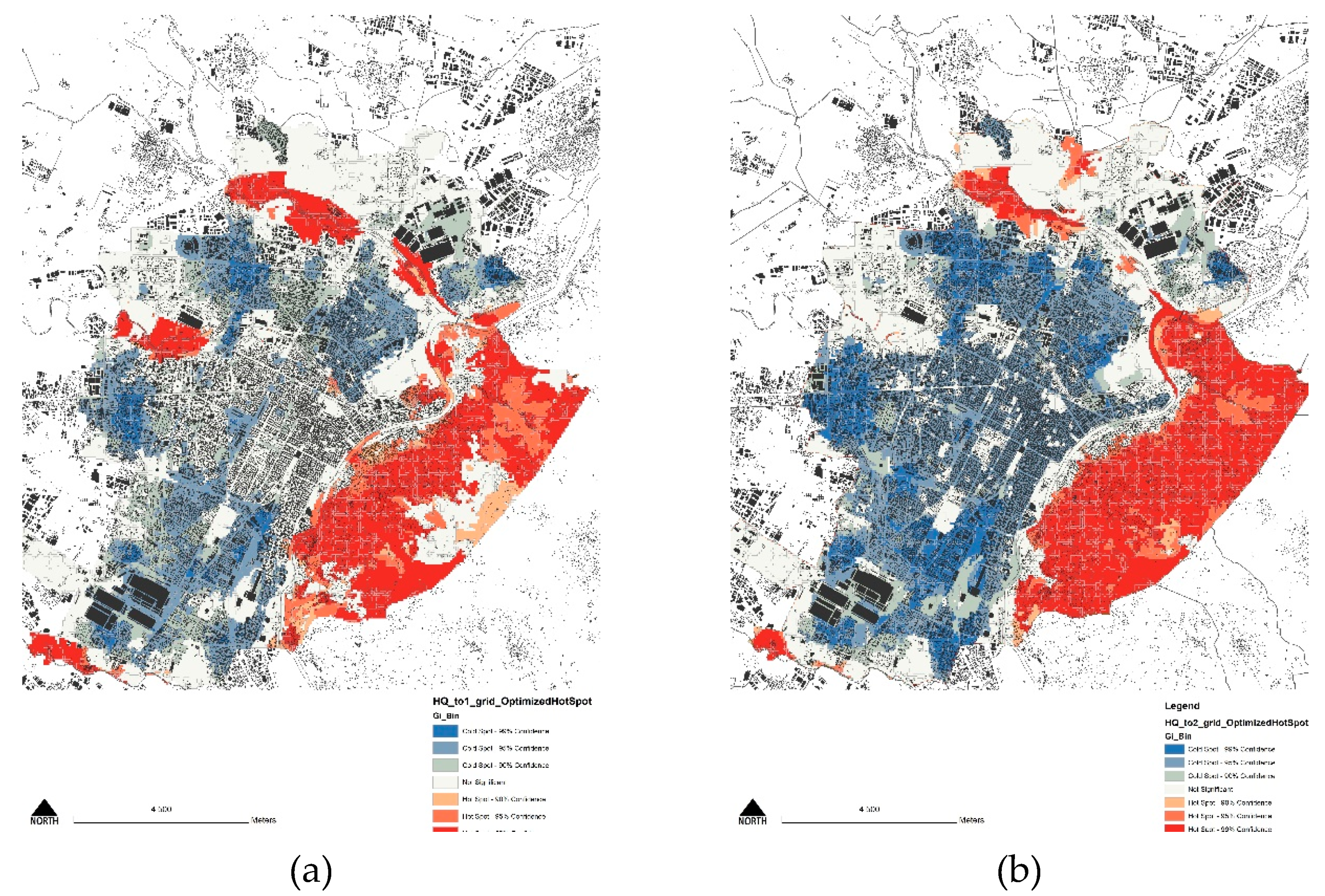
The obtained result (see Figure 7) is a map where the red color identified the well-known green areas of the city and, vice-versa, all those densely built-up spaces that are most critical from an environmental point of view.

As expected, while the most famous “green” areas (the hill, the confluence of the Po and Stura Rivers) are colored of red (clusters of high HQ values) in both outputs, the two representations differ in their “cold spots” (blue patches) and the different configuration of the “gaps” among the cold and hot spots (white areas) in the dense urban catchment.

As it can be seen in Figure 7, while in the SAM4CP output the large majority of the densely built-up area is neither a hot nor cold spot, in the NDVI-driven result, white areas are concentrated to certain points of the city, indicating that where the HQ values are not too low (cold spots), there are a few urban catchments that display “in-between” HQ values that should be graduated acknowledging a differential analysis of the environmental status in the densely built-up system.

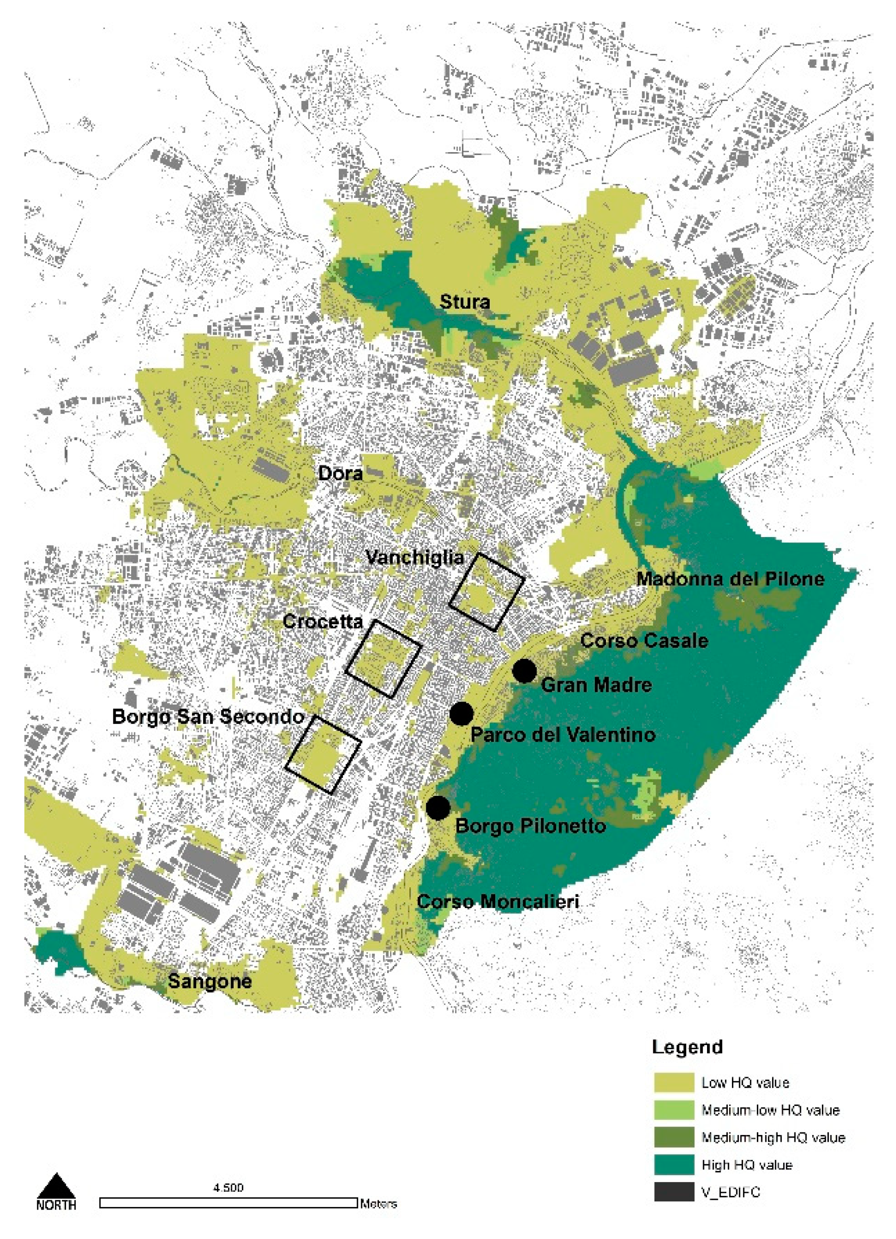
To deepen this heuristic argumentation, once the “blue” parts of the hotspot in the NDVI-driven output were removed from the map according to their statistically significant spatial autocorrelation (clusters of low HQ values), the remaining areas (red and white) were superimposed to the city base map keeping an eye on their geographical distribution in the city of Turin. The exported selection of white and red areas from the hotspot (Figure 7) was re-colored in green (Figure 8) while recognizing that the selected areas overlap the most relevant public and private urban green features that characterize the settlement system of the city. Some of these places are already included in the ecological “conservation and valorization” strategies of the city while others shape the structure and the characterization of the green infrastructure of Turin.

The Corso Casale/Corso Moncalieri axes and their connection with the city hill bordering the Po River until the Madonna del Pilone and Sassi fraction in the north and the Parco del Valentino, Borgo Pilonetto, and the Sangone River confluence in the south are among the greenest and most valuable urban-green settlements of Turin. However, the northern part along the Stura stream, even if characterized by a mixed-up productive, industrial, and logistic land use, is among the most porous urban areas of the city, with a high capability to support many ecosystem services. Finally, the Vanchiglia, Vanchiglietta, and the Crocetta with the Borgo San Secondo quarters are well-identified in the map (Figure 7) and are equally recognized as typical garden-city morphologies of the city.

The above-mentioned quarters are not to be considered properly “open-space green areas” since they represent urban features that mostly include private lots of various functions with a huge presence of healthy vegetation planted in unsealed green spaces. Nonetheless, these parts of the city are among the most valuable, characteristic, and ecosystemically-compatible of the Turin urban morphology that needs a particular planning regulation and maintenance.

The interpretation of this final analytical procedure was used to highlight some discursive considerations around the utilization of HQ results and does not pretend to contain any regulative or methodological implication while revealing that if well-inputted, the HQ can generate a different background to design UGI at the local scale. Nevertheless, the methodology reported here can be adopted in any other context where the habitat quality was modeled while looking at how a remotely sensed dataset such as the NDVI can support the re-definition of the sensitivity input table.

Far from being interpreted as a background for UGI development [1,51], this result remains of great value to support the technical knowledge of ES mapping while aiding the decision-making processes. Particularly, if the process of modeling HQ is delivered by employing site-specific datasets, such as the NDVI, then the interpretation of results is much appreciable in terms of reliability and direct utilization for designing the green network of the city.

Light and dark green areas in the above-represented image (Figure 8) are the ones that range from insignificant to positively statistically significant HQ values, whereas the light green values are the ones that include the small and medium or big public lots and private gardens of the densely built-up area with high porous and planted soil that is directly facing the settlement system and the road and infrastructural network. The medium green areas are represented by three different main typologies: the historical densely built-up area of Gran Madre that interfaces the Po River and the Turin Hill; and the inland hilly areas and some of the Po riverbanks. Finally, the dark green areas are represented by the most famous urban forests that are distributed on the city borders, at the interface between the densely built-up area and the residual rural/hilly environment around. The map recognizes well the parts of the densely built-up city that require particular attention in framing a local regulation that maximizes the ecosystem provisioning capacity.

Within this comparison, it is not our intention to indicate which is the best model, since HQ represents a relative index that does not quantify any biophysical property of the landscape; thus this empirical comparison is far from representing a sensitivity test of the HQ model to its inputs. Nonetheless, what we can observe, is that the integration of a new sensitivity score by quantitative indexing, in this case, produced a more accurate definition of the urban green network with good identification of all those parts of the city that support ecosystem functioning and structure even in small urban lots.

5. Conclusions

Often obtaining ES modeling results is not enough to pose effective support while designing landscape plans and UGI at the local level [7,45,51].

The scientific improvement of the relations between input/output of modeling can improve ES assessment, especially when outputs are used to improve real urban planning processes. This manuscript tried to empirically test two outputs of habitat quality modeling using different sensitivity values [6,52,53].

Results demonstrate that while, at first, the results seem to be less representative in supporting the heuristic argumentation around the ecological situation of the compact city of Turin, after a detailed analysis of statistics, the new NDVI-driven output provides a more comprehensive and finer frequency of habitat values at the urban catchment level. The increased frequency of HQ classification allowed to identify by hotspot extraction those areas that can be employed to frame a green network in the city [30,54].

Far away from identifying the NDVI as the best input indicator for HQ modeling, this empirical test demonstrated that site-specific urban datasets are highly relevant to provide different modeling results. This achievement should be evaluated not as an alternative to the traditional modeling method but as a complementary one while answering the need of expanding the practical experience around HQ modeling which is still far from being reached.

We are aware that the NDVI has several limitations in being used to set the sensitivity since the health of vegetation does not represent the suitability to keep biodiversity and support the development of various habitats for different flora and fauna species. Nonetheless, if well-used, this indicator can be employed to adjust/correct/implement the input parameters while obtaining a higher statistical differentiation of the output.

Within this heuristic argumentation, we want to encourage also the contemporary research on urban ecosystems to trace further steps in providing differentiated solutions, while overcoming the traditional macro-evaluation of urban green spaces. Therefore, we encourage the testing of the methodology in similar contexts of study where compact and dense urban areas are surrounded by an extensive peri-urban system while preserving an internal characterization of open spaces with different degrees of ecological quality. Within a growing number of comparative results, we can link this experience with other potential research and planning projects while filling the gap between theoretical and practical utilization of ES in planning.