Seismic Vulnerability Assessment and Mapping of Gyeongju, South Korea Using Frequency Ratio, Decision Tree, and Random Forest


Abstract
:1. Introduction
2. Study Area and Data
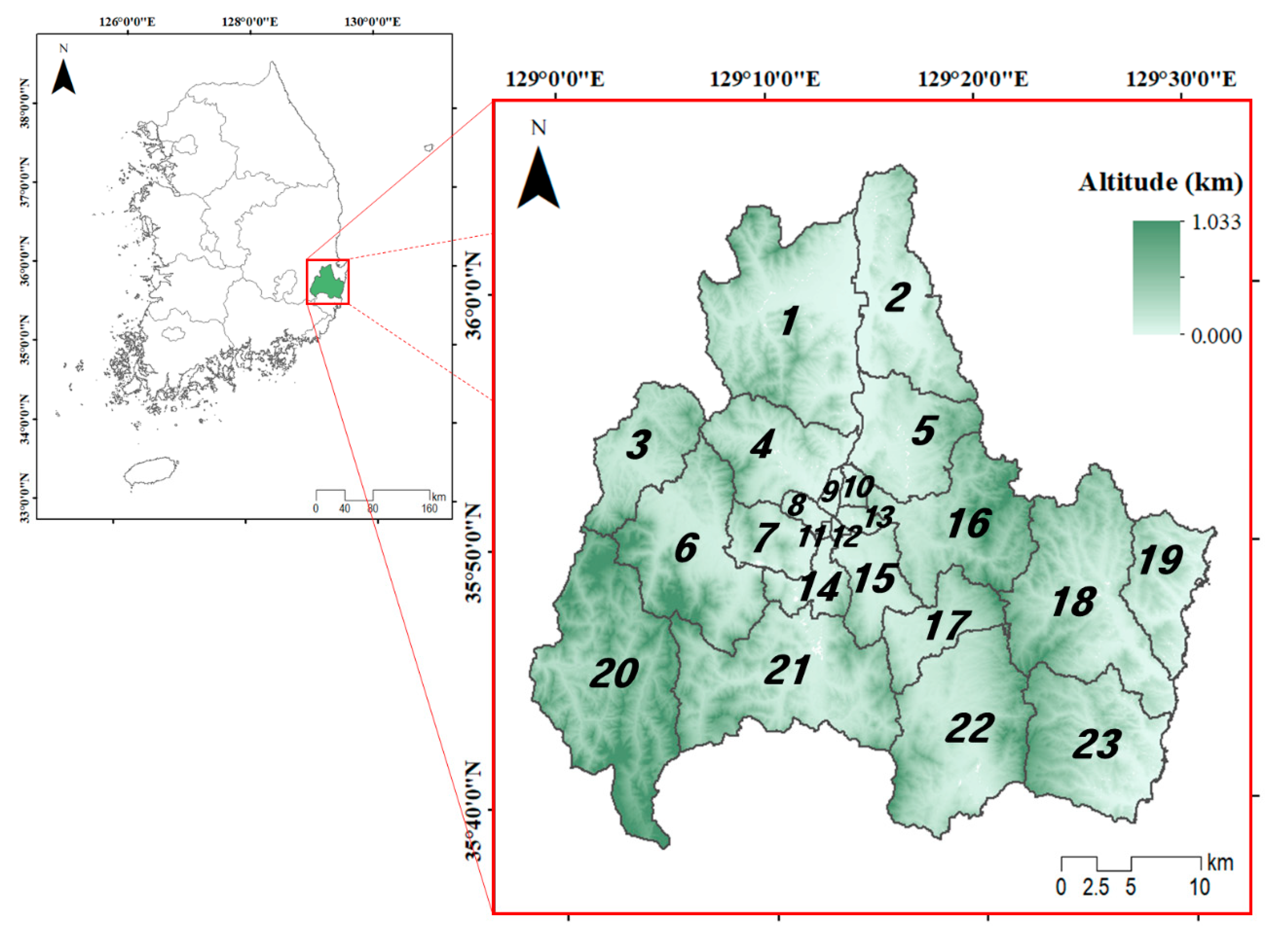
2.1. Study Area
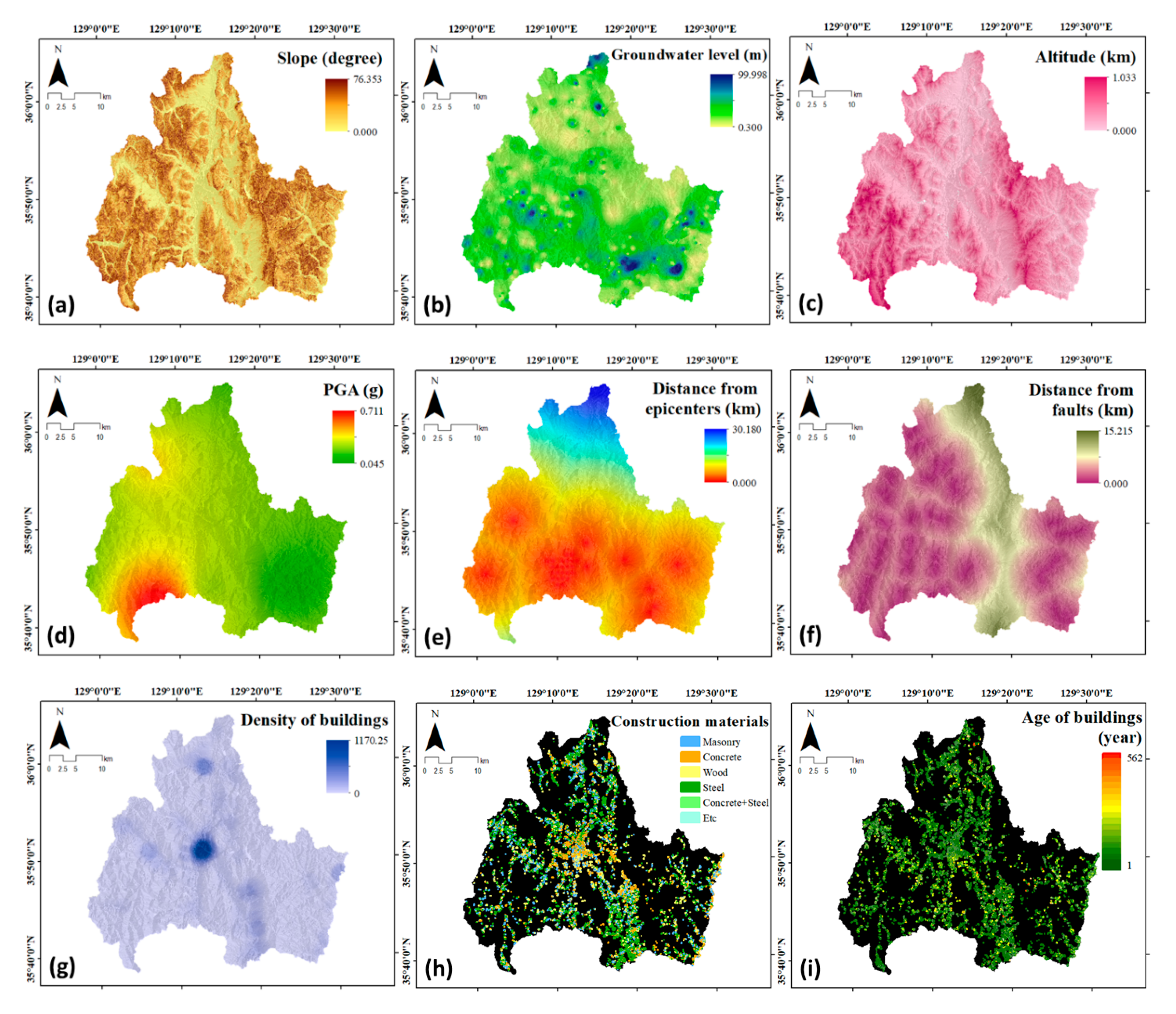
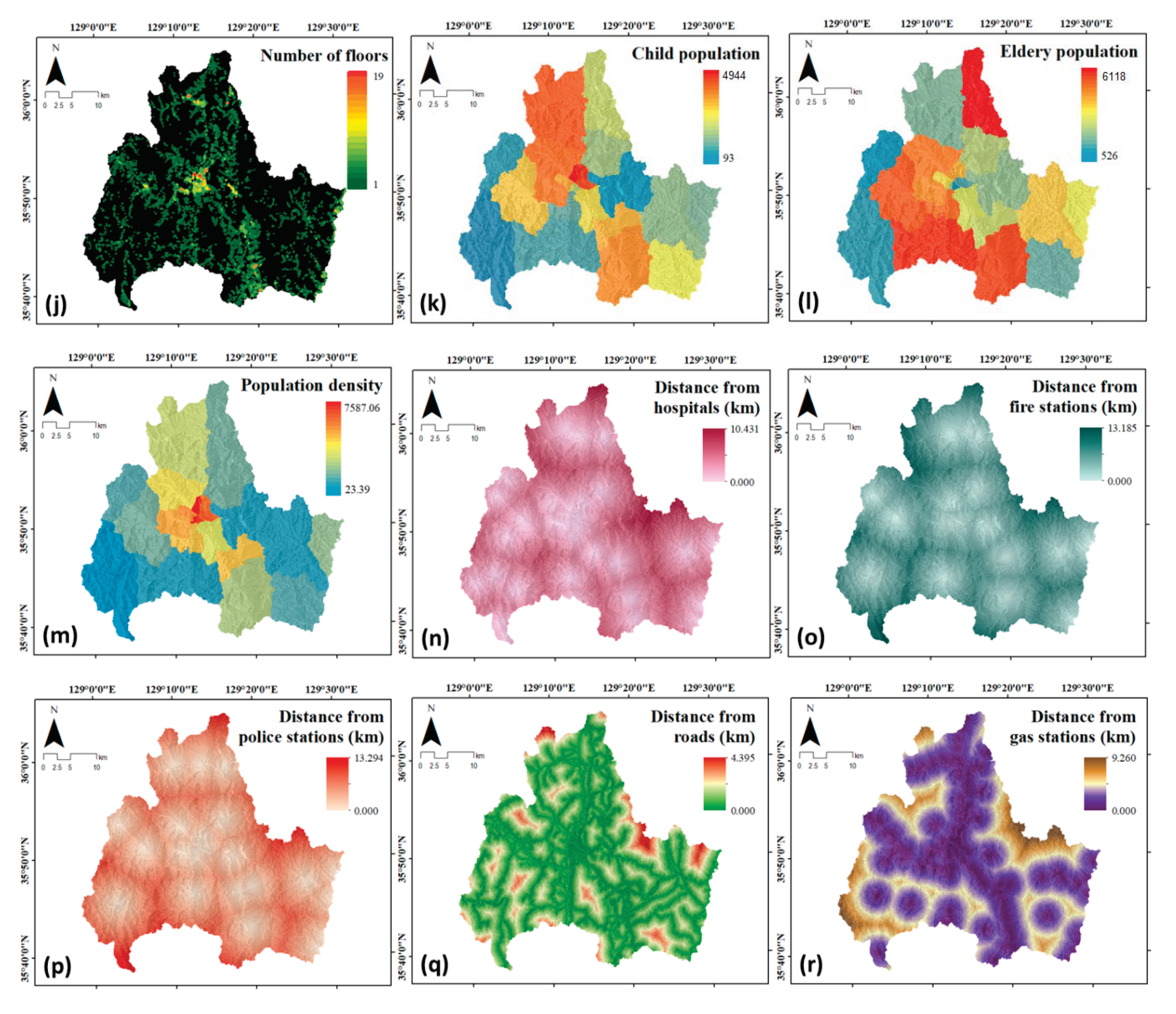
2.2. Data
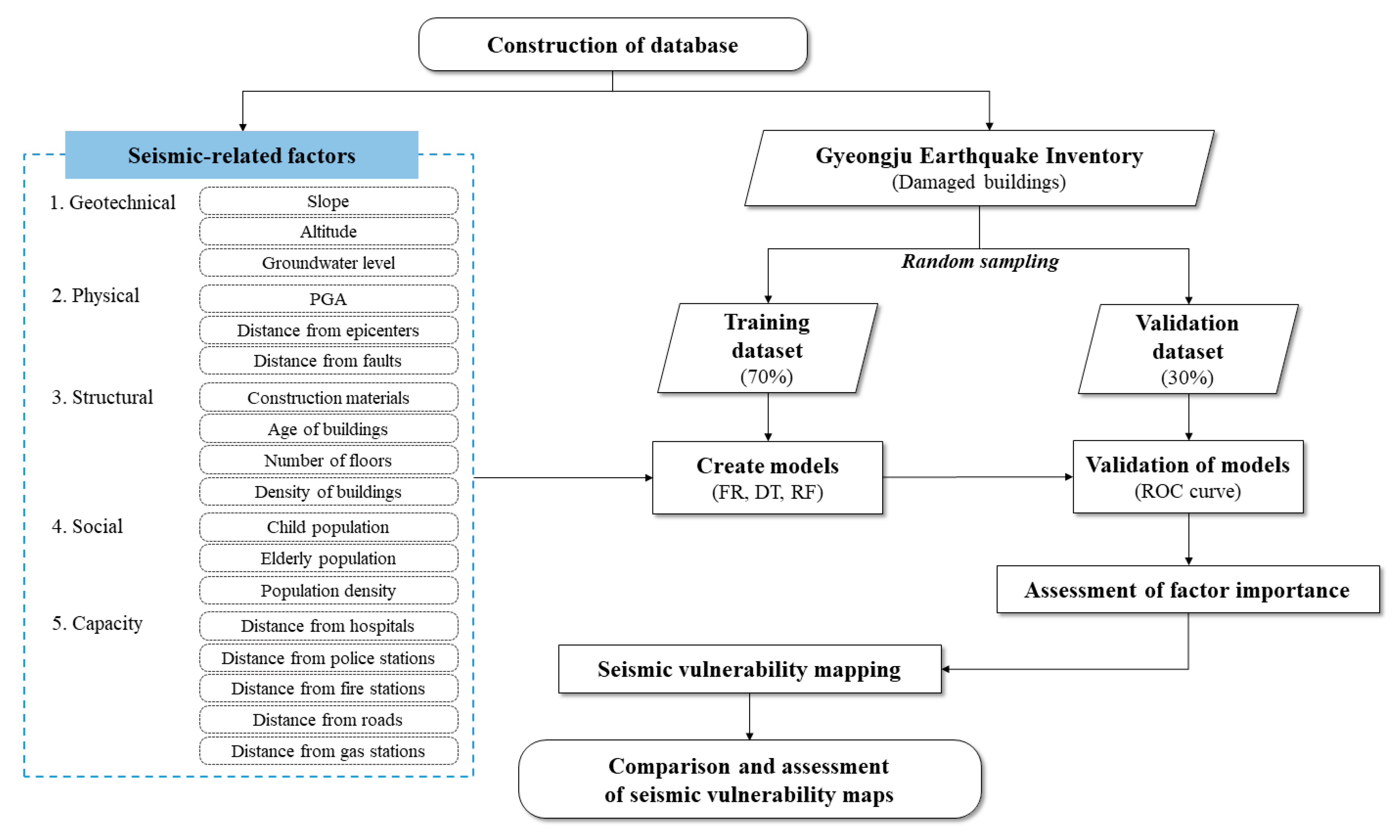
3. Methodology
3.1. FR Model
- TGFC: Training Grid of Factor Class
- WTG: Whole Training Grid
- FC: Factor Class Grid
- WG: Whole Grid
3.2. DT Model
3.3. RF Model
3.4. Assessment of Model Performance
4. Results
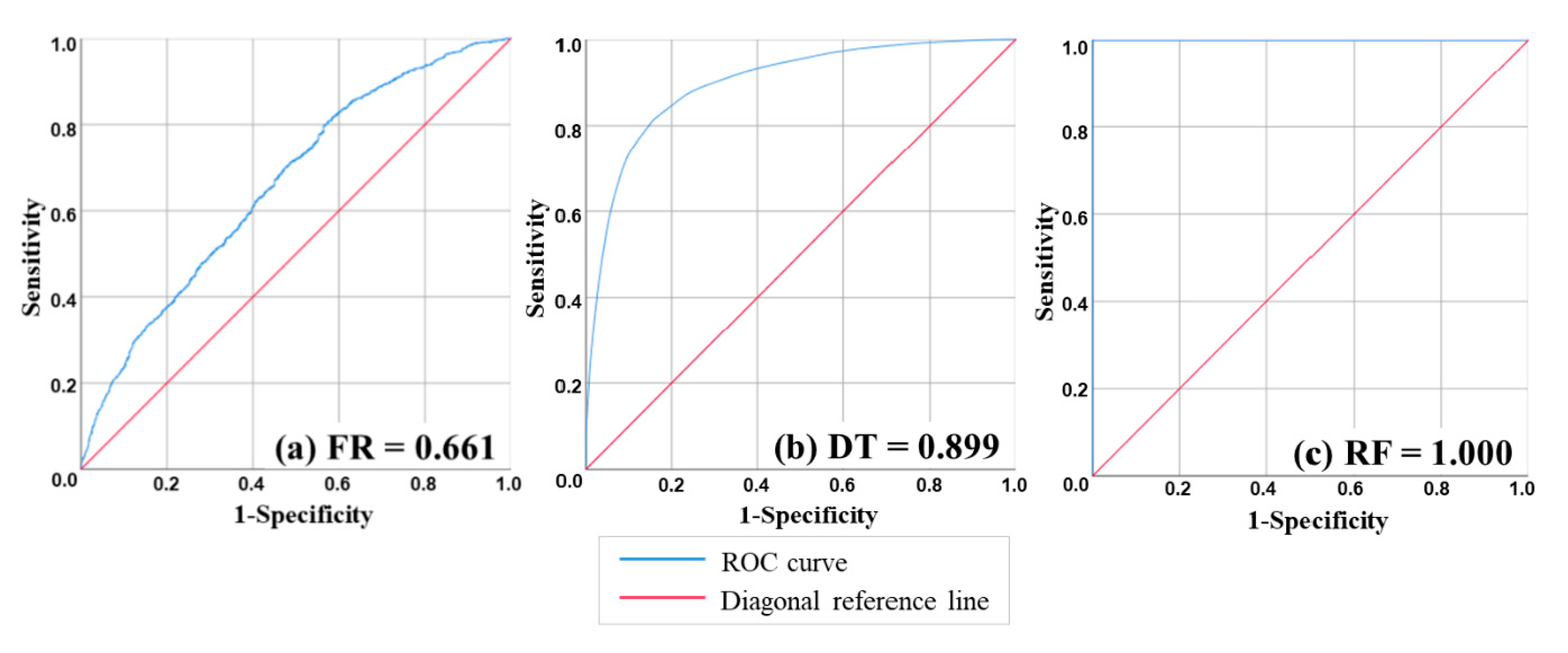
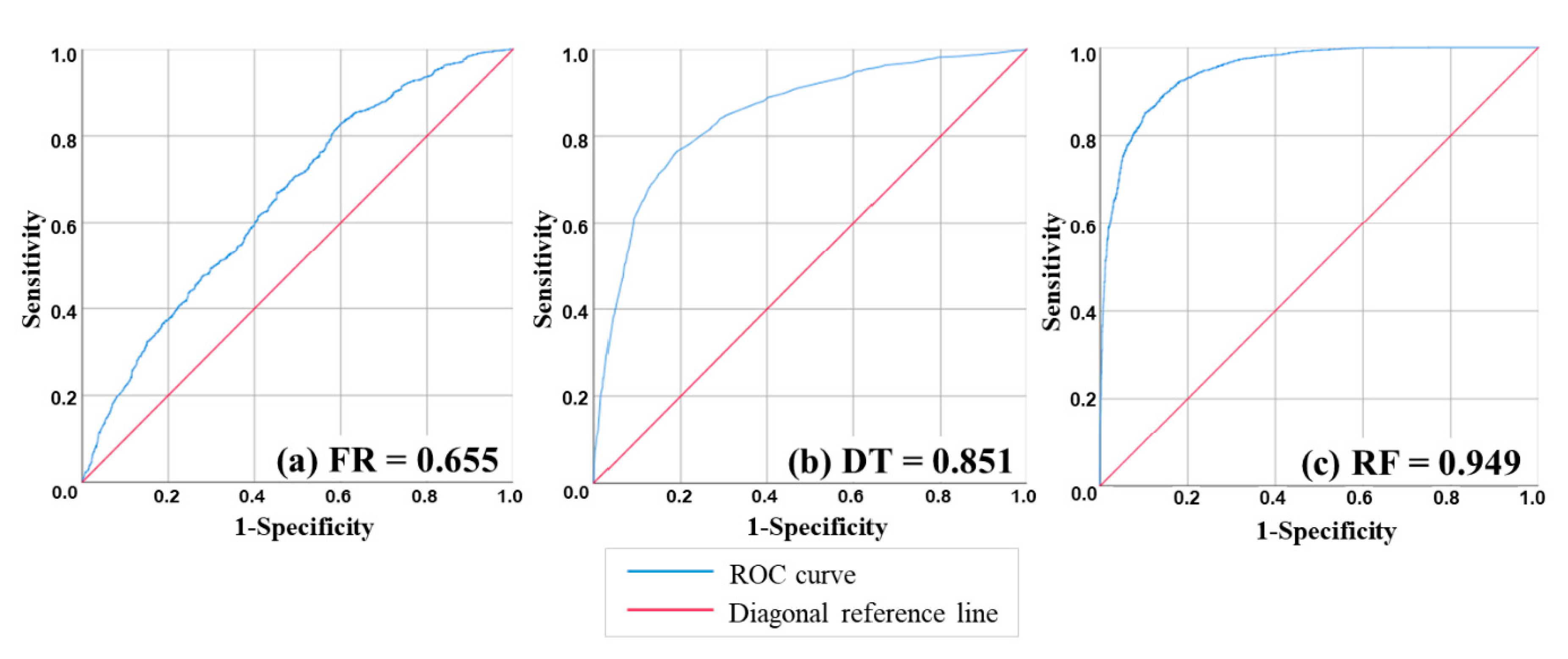
4.1. Model Validation and Comparison
4.2. Relative Importance of Factors
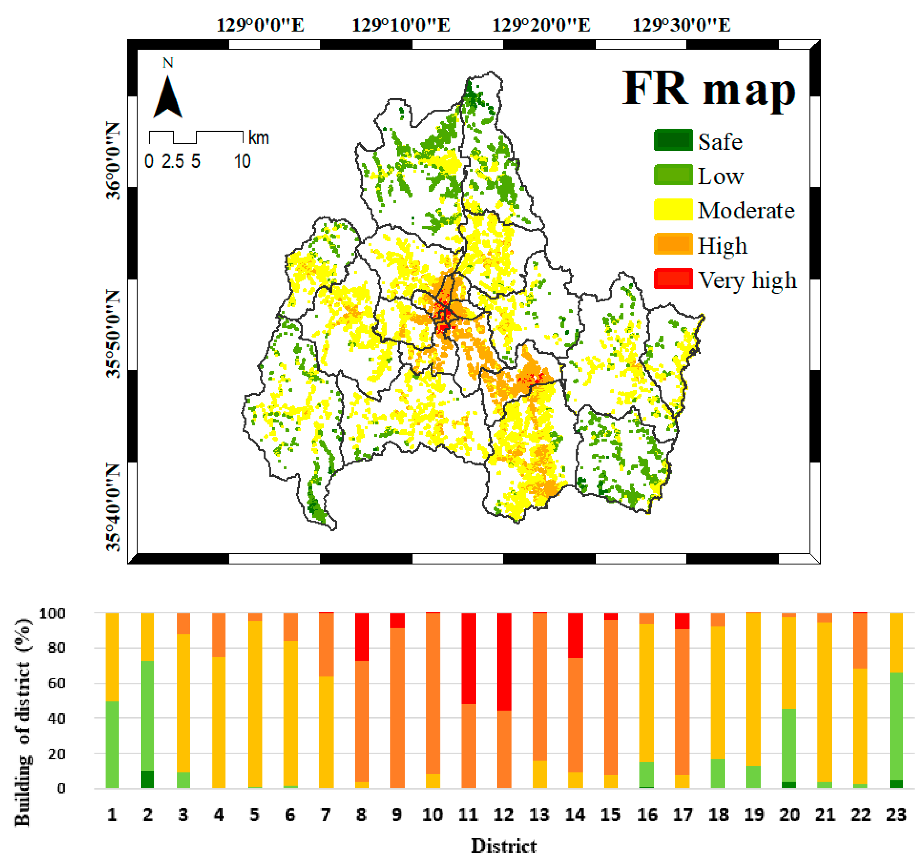
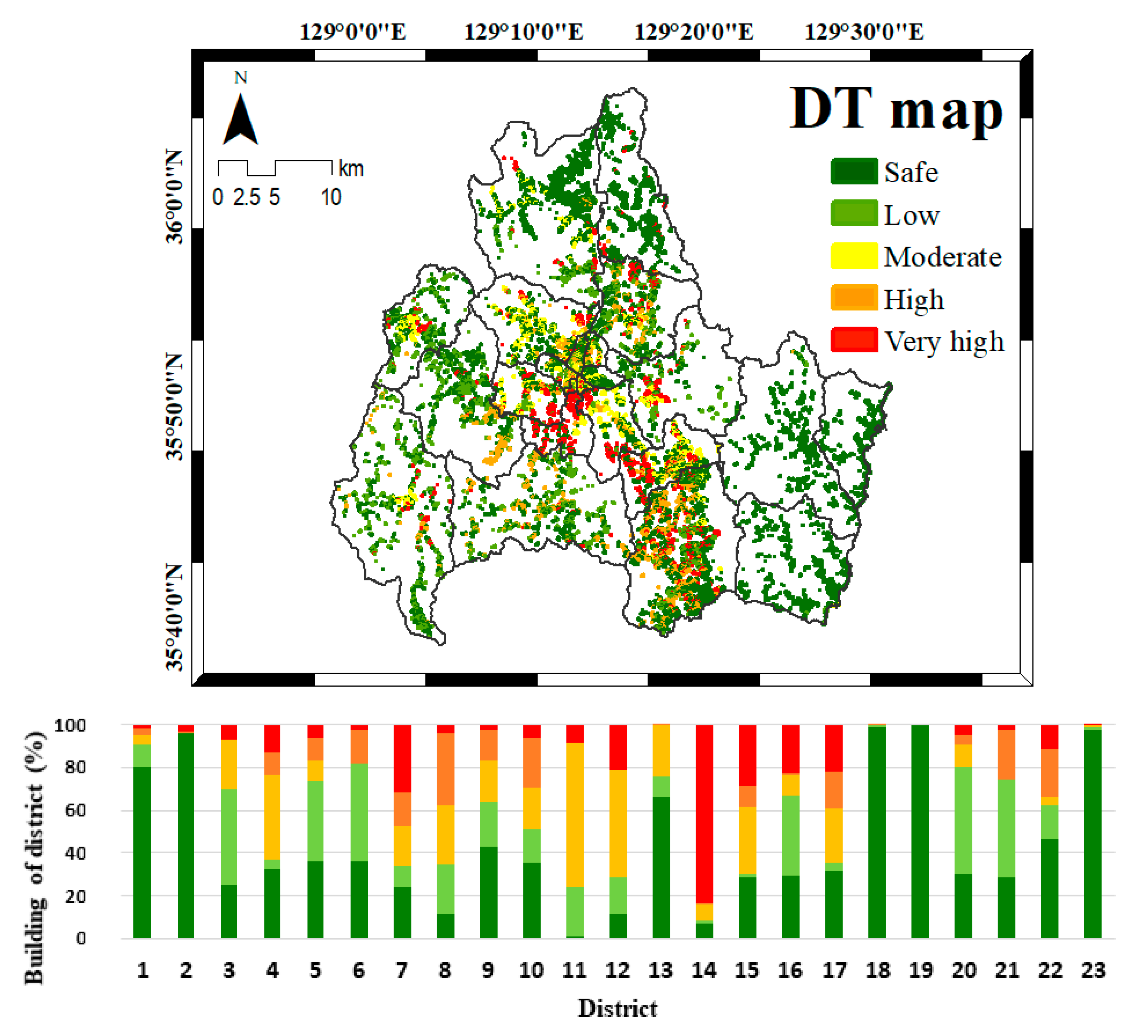
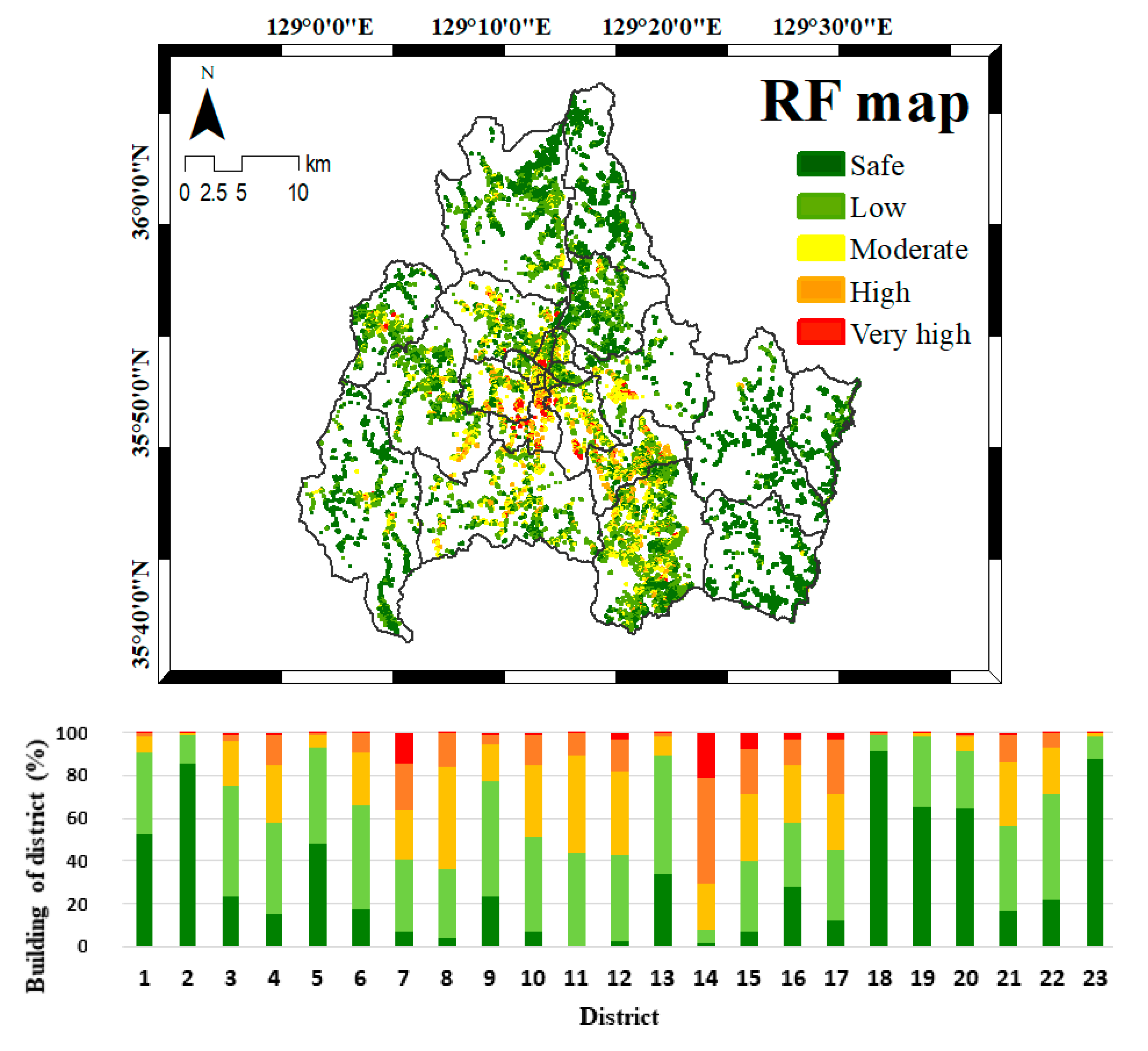
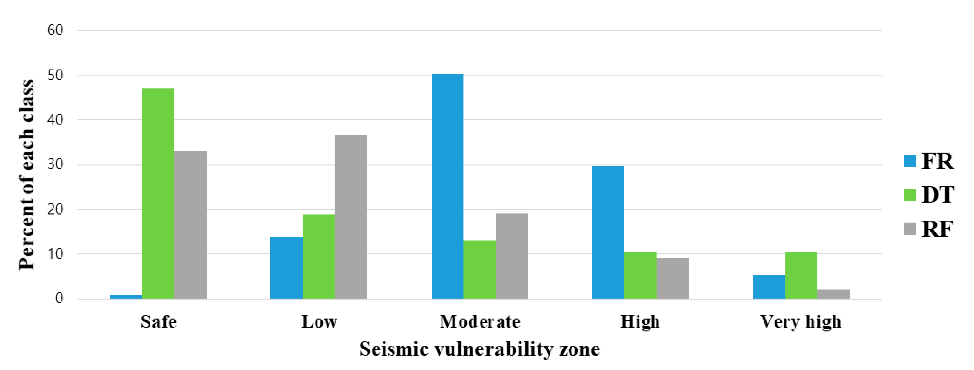
4.3. Seismic Vulnerability Mapping
5. Discussion
6. Conclusions
Author Contributions
Funding
Acknowledgments
Conflicts of Interest
References
- Kim, Y.; Rhie, J.; Kang, T.S.; Kim, K.H.; Kim, M.; Lee, S.J. The 12 September 2016 Gyeongju Earthquakes: 1. Observation and Remaining Questions. Geosci. J. 2016, 20, 747–752. [Google Scholar] [CrossRef]
- Kim, K.H.; Kang, T.S.; Rhie, J.; Kim, Y.; Park, Y.; Kang, S.Y.; Han, M.; Kim, J.; Park, J.; Kim, M. The 12 September 2016 Gyeongju Earthquakes: 2. Temporary Seismic Network for Monitoring Aftershocks. Geosci. J. 2016, 20, 753–757. [Google Scholar] [CrossRef]
- Ministry of Public Safety and Security (MPSS). Report on the 9.12 Earthquake and Countermeasures; MPSS: Seoul, Korea, 2017.
- Wallemacq, P. Economic Losses, Poverty & Disasters: 1998–2017; Centre for Research on the Epidemiology of Disasters: Brussels, Belgium, 2018. [Google Scholar]
- Armaş, I. Multi-Criteria Vulnerability Analysis to Earthquake Hazard of Bucharest, Romania. Nat. Hazards 2012, 63, 1129–1156. [Google Scholar] [CrossRef]
- Walker, B.B.; Taylor-Noonan, C.; Tabbernor, A.; Bal, H.; Bradley, D.; Schuurman, N.; Clague, J.J. A Multi-Criteria Evaluation Model of Earthquake Vulnerability in Victoria, British Columbia. Nat. Hazards 2014, 74, 1209–1222. [Google Scholar] [CrossRef]
- Sadrykia, M.; Delavar, M.R.; Zare, M. A GIS-Based Decision Making Model using Fuzzy Sets and Theory of Evidence for Seismic Vulnerability Assessment Under Uncertainty (Case Study: Tabriz). J. Intell. Fuzzy Syst. 2017, 33, 1969–1981. [Google Scholar] [CrossRef] [Green Version]
- Panahi, M.; Rezaie, F.; Meshkani, S. Seismic Vulnerability Assessment of School Buildings in Tehran City Based on AHP and GIS. Nat. Hazards Earth Syst. Sci. 2014, 14, 969–979. [Google Scholar] [CrossRef] [Green Version]
- Nath, S.; Adhikari, M.; Devaraj, N.; Maiti, S. Seismic Vulnerability and Risk Assessment of Kolkata City, India. Nat. Hazards Earth Syst. Sci. 2015, 15, 1103. [Google Scholar] [CrossRef] [Green Version]
- Rezaie, F.; Panahi, M. GIS Modeling of Seismic Vulnerability of Residential Fabrics Considering Geotechnical, Structural, Social and Physical Distance Indicators in Tehran using Multi-Criteria Decision-Making Techniques. Nat. Hazards Earth Syst. Sci. 2015, 15, 461–474. [Google Scholar] [CrossRef] [Green Version]
- Bahadori, H.; Hasheminezhad, A.; Karimi, A. Development of an Integrated Model for Seismic Vulnerability Assessment of Residential Buildings: Application to Mahabad City, Iran. J. Build. Eng. 2017, 12, 118–131. [Google Scholar] [CrossRef]
- Alizadeh, M.; Alizadeh, E.; Asadollahpour Kotenaee, S.; Shahabi, H.; Beiranvand Pour, A.; Panahi, M.; Bin Ahmad, B.; Saro, L. Social Vulnerability Assessment using Artificial Neural Network (ANN) Model for Earthquake Hazard in Tabriz City, Iran. Sustainability 2018, 10, 3376. [Google Scholar] [CrossRef] [Green Version]
- Moradi, M.; Delavar, M.R.; Moshiri, B. A GIS-Based Multi-Criteria Decision-Making Approach for Seismic Vulnerability Assessment using Quantifier-Guided OWA Operator: A Case Study of Tehran, Iran. Ann. GIS 2015, 21, 209–222. [Google Scholar] [CrossRef]
- Nyimbili, P.H.; Erden, T.; Karaman, H. Integration of GIS, AHP and TOPSIS for Earthquake Hazard Analysis. Nat. Hazards 2018, 92, 1523–1546. [Google Scholar] [CrossRef]
- Alam, M.S.; Haque, S.M. Assessment of Urban Physical Seismic Vulnerability using the Combination of AHP and TOPSIS Models: A Case Study of Residential Neighborhoods of Mymensingh City, Bangladesh. J. Geosci. Environ. Prot. 2018, 6, 165. [Google Scholar] [CrossRef] [Green Version]
- Lee, S.; Panahi, M.; Pourghasemi, H.R.; Shahabi, H.; Alizadeh, M.; Shirzadi, A.; Khosravi, K.; Melesse, A.M.; Yekrangnia, M.; Rezaie, F. Sevucas: A Novel Gis-Based Machine Learning Software for Seismic Vulnerability Assessment. Appl. Sci. 2019, 9, 3495. [Google Scholar] [CrossRef] [Green Version]
- Yariyan, P.; Avand, M.; Soltani, F.; Ghorbanzadeh, O.; Blaschke, T. Earthquake Vulnerability Mapping using Different Hybrid Models. Symmetry 2020, 12, 405. [Google Scholar] [CrossRef] [Green Version]
- Riedel, I.; Guéguen, P.; Dalla Mura, M.; Pathier, E.; Leduc, T.; Chanussot, J. Seismic Vulnerability Assessment of Urban Environments in Moderate-to-Low Seismic Hazard Regions using Association Rule Learning and Support Vector Machine Methods. Nat. Hazards 2015, 76, 1111–1141. [Google Scholar] [CrossRef]
- Guettiche, A.; Guéguen, P.; Mimoune, M. Seismic Vulnerability Assessment using Association Rule Learning: Application to the City of Constantine, Algeria. Nat. Hazards 2017, 86, 1223–1245. [Google Scholar] [CrossRef]
- Han, J.; Park, S.; Kim, S.; Son, S.; Lee, S.; Kim, J. Performance of Logistic Regression and Support Vector Machines for Seismic Vulnerability Assessment and Mapping: A Case Study of the 12 September 2016 ML5. 8 Gyeongju Earthquake, South Korea. Sustainability 2019, 11, 7038. [Google Scholar] [CrossRef] [Green Version]
- Liu, Y.; Li, Z.; Wei, B.; Li, X.; Fu, B. Seismic Vulnerability Assessment at Urban Scale using Data Mining and GIScience Technology: Application to Urumqi (China). Geomat. Nat. Hazards Risk 2019, 10, 958–985. [Google Scholar] [CrossRef] [Green Version]
- Youssef, A.M.; Pradhan, B.; Sefry, S.A. Flash Flood Susceptibility Assessment in Jeddah City (Kingdom of Saudi Arabia) using Bivariate and Multivariate Statistical Models. Environ. Earth Sci. 2016, 75, 12. [Google Scholar] [CrossRef]
- Al-Abadi, A.M. Mapping Flood Susceptibility in an Arid Region of Southern Iraq using Ensemble Machine Learning Classifiers: A Comparative Study. Arab. J. Geosci. 2018, 11, 218. [Google Scholar] [CrossRef]
- Choubin, B.; Moradi, E.; Golshan, M.; Adamowski, J.; Sajedi-Hosseini, F.; Mosavi, A. An Ensemble Prediction of Flood Susceptibility using Multivariate Discriminant Analysis, Classification and Regression Trees, and Support Vector Machines. Sci. Total Environ. 2019, 651, 2087–2096. [Google Scholar] [CrossRef]
- Tehrany, M.S.; Kumar, L.; Shabani, F. A Novel GIS-Based Ensemble Technique for Flood Susceptibility Mapping using Evidential Belief Function and Support Vector Machine: Brisbane, Australia. PeerJ 2019, 7, e7653. [Google Scholar] [CrossRef] [PubMed]
- Chen, W.; Li, Y.; Xue, W.; Shahabi, H.; Li, S.; Hong, H.; Wang, X.; Bian, H.; Zhang, S.; Pradhan, B. Modeling Flood Susceptibility using Data-Driven Approaches of Naïve Bayes Tree, Alternating Decision Tree, and Random Forest Methods. Sci. Total Environ. 2020, 701, 134979. [Google Scholar] [CrossRef] [PubMed]
- Yalcin, A.; Reis, S.; Aydinoglu, A.C.; Yomralioglu, T. A GIS-Based Comparative Study of Frequency Ratio, Analytical Hierarchy Process, Bivariate Statistics and Logistics Regression Methods for Landslide Susceptibility Mapping in Trabzon, NE Turkey. Catena 2011, 85, 274–287. [Google Scholar] [CrossRef]
- Bui, D.T.; Tuan, T.A.; Klempe, H.; Pradhan, B.; Revhaug, I. Spatial Prediction Models for Shallow Landslide Hazards: A Comparative Assessment of the Efficacy of Support Vector Machines, Artificial Neural Networks, Kernel Logistic Regression, and Logistic Model Tree. Landslides 2016, 13, 361–378. [Google Scholar]
- Youssef, A.M.; Pourghasemi, H.R.; Pourtaghi, Z.S.; Al-Katheeri, M.M. Landslide Susceptibility Mapping using Random Forest, Boosted Regression Tree, Classification and Regression Tree, and General Linear Models and Comparison of their Performance at Wadi Tayyah Basin, Asir Region, Saudi Arabia. Landslides 2016, 13, 839–856. [Google Scholar] [CrossRef]
- Shrestha, S.; Kang, T.; Suwal, M. An Ensemble Model for Co-Seismic Landslide Susceptibility using GIS and Random Forest Method. ISPRS Int. J. Geo-Inf. 2017, 6, 365. [Google Scholar] [CrossRef] [Green Version]
- Park, S.; Hamm, S.; Kim, J. Performance Evaluation of the Gis-Based Data-Mining Techniques Decision Tree, Random Forest, and Rotation Forest for Landslide Susceptibility Modeling. Sustainability 2019, 11, 5659. [Google Scholar] [CrossRef] [Green Version]
- Wang, Y.; Wu, X.; Chen, Z.; Ren, F.; Feng, L.; Du, Q. Optimizing the Predictive Ability of Machine Learning Methods for Landslide Susceptibility Mapping using Smote for Lishui City in Zhejiang Province, China. Int. J. Environ. Res. Public Health 2019, 16, 368. [Google Scholar] [CrossRef] [Green Version]
- Nhu, V.; Shirzadi, A.; Shahabi, H.; Chen, W.; Clague, J.J.; Geertsema, M.; Jaafari, A.; Avand, M.; Miraki, S.; Talebpour Asl, D. Shallow Landslide Susceptibility Mapping by Random Forest Base Classifier and its Ensembles in a Semi-Arid Region of Iran. Forests 2020, 11, 421. [Google Scholar] [CrossRef] [Green Version]
- Nhu, V.; Shirzadi, A.; Shahabi, H.; Singh, S.K.; Al-Ansari, N.; Clague, J.J.; Jaafari, A.; Chen, W.; Miraki, S.; Dou, J. Shallow Landslide Susceptibility Mapping: A Comparison between Logistic Model Tree, Logistic Regression, Naïve Bayes Tree, Artificial Neural Network, and Support Vector Machine Algorithms. Int. J. Environ. Res. Public Health 2020, 17, 2749. [Google Scholar] [CrossRef]
- Avand, M.; Janizadeh, S.; Naghibi, S.A.; Pourghasemi, H.R.; Khosrobeigi Bozchaloei, S.; Blaschke, T. A Comparative Assessment of Random Forest and k-Nearest Neighbor Classifiers for Gully Erosion Susceptibility Mapping. Water 2019, 11, 2076. [Google Scholar] [CrossRef] [Green Version]
- Garosi, Y.; Sheklabadi, M.; Conoscenti, C.; Pourghasemi, H.R.; Van Oost, K. Assessing the Performance of GIS-Based Machine Learning Models with Different Accuracy Measures for Determining Susceptibility to Gully Erosion. Sci. Total Environ. 2019, 664, 1117–1132. [Google Scholar] [CrossRef]
- Pourghasemi, H.R.; Yousefi, S.; Kornejady, A.; Cerdà, A. Performance Assessment of Individual and Ensemble Data-Mining Techniques for Gully Erosion Modeling. Sci. Total Environ. 2017, 609, 764–775. [Google Scholar] [CrossRef] [PubMed] [Green Version]
- Tien Bui, D.; Shirzadi, A.; Shahabi, H.; Chapi, K.; Omidavr, E.; Pham, B.T.; Talebpour Asl, D.; Khaledian, H.; Pradhan, B.; Panahi, M. A Novel Ensemble Artificial Intelligence Approach for Gully Erosion Mapping in a Semi-Arid Watershed (Iran). Sensors 2019, 19, 2444. [Google Scholar] [CrossRef] [PubMed] [Green Version]
- Nhu, V.; Janizadeh, S.; Avand, M.; Chen, W.; Farzin, M.; Omidvar, E.; Shirzadi, A.; Shahabi, H.; Clague, J.J.; Jaafari, A. Gis-Based Gully Erosion Susceptibility Mapping: A Comparison of Computational Ensemble Data Mining Models. Appl. Sci. 2020, 10, 2039. [Google Scholar] [CrossRef] [Green Version]
- Miraki, S.; Zanganeh, S.H.; Chapi, K.; Singh, V.P.; Shirzadi, A.; Shahabi, H.; Pham, B.T. Mapping Groundwater Potential using a Novel Hybrid Intelligence Approach. Water Resour. Manag. 2019, 33, 281–302. [Google Scholar] [CrossRef]
- Nhu, V.; Rahmati, O.; Falah, F.; Shojaei, S.; Al-Ansari, N.; Shahabi, H.; Shirzadi, A.; Górski, K.; Nguyen, H.; Ahmad, B.B. Mapping of Groundwater Spring Potential in Karst Aquifer System using Novel Ensemble Bivariate and Multivariate Models. Water 2020, 12, 985. [Google Scholar] [CrossRef] [Green Version]
- Tien Bui, D.; Shirzadi, A.; Chapi, K.; Shahabi, H.; Pradhan, B.; Pham, B.T.; Singh, V.P.; Chen, W.; Khosravi, K.; Bin Ahmad, B. A Hybrid Computational Intelligence Approach to Groundwater Spring Potential Mapping. Water 2019, 11, 2013. [Google Scholar] [CrossRef] [Green Version]
- Chen, W.; Li, Y.; Tsangaratos, P.; Shahabi, H.; Ilia, I.; Xue, W.; Bian, H. Groundwater Spring Potential Mapping using Artificial Intelligence Approach Based on Kernel Logistic Regression, Random Forest, and Alternating Decision Tree Models. Appl. Sci. 2020, 10, 425. [Google Scholar] [CrossRef] [Green Version]
- Chen, W.; Zhao, X.; Tsangaratos, P.; Shahabi, H.; Ilia, I.; Xue, W.; Wang, X.; Ahmad, B.B. Evaluating the Usage of Tree-Based Ensemble Methods in Groundwater Spring Potential Mapping. J. Hydrol. 2020, 583, 124602. [Google Scholar] [CrossRef]
- Şengezer, B.; Ansal, A.; Bilen, Ö. Evaluation of Parameters Affecting Earthquake Damage by Decision Tree Techniques. Nat. Hazards 2008, 47, 547–568. [Google Scholar] [CrossRef]
- Borfecchia, F.; De Cecco, L.; Pollino, M.; La Porta, L.; Lugari, A.; Martini, S.; Ristoratore, E.; Pascale, C. Active and Passive Remote Sensing for Supporting the Evaluation of the Urban Seismic Vulnerability. Ital. J. Remote Sens. 2010, 42, 129–141. [Google Scholar] [CrossRef]
- Ahmed, M.; Morita, H. An Analysis of Housing Structures’ Earthquake Vulnerability in Two Parts of Dhaka City. Sustainability 2018, 10, 1106. [Google Scholar] [CrossRef] [Green Version]
- Gyeongju City Hall. Available online: http://www.gyeongju.go.kr/ (accessed on 10 March 2020).
- Korea Meteorological Administration. Available online: http://www.weather.go.kr/ (accessed on 17 March 2020).
- Kim, Y.; Kim, T.; Kyung, J.B.; Cho, C.S.; Choi, J.; Choi, C.U. Preliminary Study on Rupture Mechanism of the 9.12 Gyeongju Earthquake. J. Geol. Soc. Korea 2017, 53, 407–422. [Google Scholar] [CrossRef]
- Han, J.; Kim, J. A GIS-Based Seismic Vulnerability Mapping and Assessment using AHP: A Case Study of Gyeongju, Korea. Korean J. Remote Sens. 2019, 35, 217–228. [Google Scholar]
- Lee, M.; Kang, J. Predictive Flooded Area Susceptibility and Verification using GIS and Frequency Ratio. J. Korean Assoc. Geogr. Inf. Stud. 2012, 15, 86–102. [Google Scholar] [CrossRef] [Green Version]
- Son, J. Susceptibility Assessment of Landslide and Land Subsidence Applying the Radius of Influence to Frequency Ratio Model. Ph.D. Thesis, Graduate School of Seoul National University, Seoul, Korea, 2017. [Google Scholar]
- Wang, L.; Guo, M.; Sawada, K.; Lin, J.; Zhang, J. A Comparative Study of Landslide Susceptibility Maps using Logistic Regression, Frequency Ratio, Decision Tree, Weights of Evidence and Artificial Neural Network. Geosci. J. 2016, 20, 117–136. [Google Scholar] [CrossRef]
- Saito, H.; Nakayama, D.; Matsuyama, H. Comparison of Landslide Susceptibility Based on a Decision-Tree Model and Actual Landslide Occurrence: The Akaishi Mountains, Japan. Geomorphology 2009, 109, 108–121. [Google Scholar] [CrossRef]
- Pradhan, B. A Comparative Study on the Predictive Ability of the Decision Tree, Support Vector Machine and Neuro-Fuzzy Models in Landslide Susceptibility Mapping using GIS. Comput. Geosci. 2013, 51, 350–365. [Google Scholar] [CrossRef]
- Breiman, L.; Friedman, J.; Stone, C.J.; Olshen, R.A. Classification and Regression Trees; CRC Press: Boca Raton, FL, USA, 1984. [Google Scholar]
- Choi, J.; Seo, D. Application of Data Mining Decision Tree. Res. Stat. Anal. 1999, 4, 61–83. [Google Scholar]
- Kavzoglu, T.; Sahin, E.K.; Colkesen, I. An Assessment of Multivariate and Bivariate Approaches in Landslide Susceptibility Mapping: A Case Study of Duzkoy District. Nat. Hazards 2015, 76, 471–496. [Google Scholar] [CrossRef]
- Chen, W.; Xie, X.; Wang, J.; Pradhan, B.; Hong, H.; Bui, D.T.; Duan, Z.; Ma, J. A Comparative Study of Logistic Model Tree, Random Forest, and Classification and Regression Tree Models for Spatial Prediction of Landslide Susceptibility. Catena 2017, 151, 147–160. [Google Scholar] [CrossRef] [Green Version]
- Breiman, L. Random Forests. Mach. Learn. 2001, 45, 5–32. [Google Scholar] [CrossRef] [Green Version]
- Liaw, A.; Wiener, M. Classification and Regression by randomForest. R News 2002, 2, 18–22. [Google Scholar]
- Park, S.; Kim, J. Landslide Susceptibility Mapping Based on Random Forest and Boosted Regression Tree Models, and a Comparison of their Performance. Appl. Sci. 2019, 9, 942. [Google Scholar] [CrossRef] [Green Version]
- Kavzoglu, T.; Colkesen, I.; Sahin, E.K. Machine learning techniques in landslide susceptibility mapping: A survey and a case study. In Landslides: Theory, Practice and Modelling; Springer: Cham, Switzerland, 2019; pp. 283–301. [Google Scholar]
- Kim, J.; Lee, S.; Jung, H.; Lee, S. Landslide Susceptibility Mapping using Random Forest and Boosted Tree Models in Pyeong-Chang, Korea. Geocarto Int. 2018, 33, 1000–1015. [Google Scholar] [CrossRef]
- Taalab, K.; Cheng, T.; Zhang, Y. Mapping Landslide Susceptibility and Types using Random Forest. Big Earth Data 2018, 2, 159–178. [Google Scholar] [CrossRef]
- Paul, S.S.; Li, J.; Li, Y.; Shen, L. Assessing Land use–land Cover Change and Soil Erosion Potential using a Combined Approach through Remote Sensing, RUSLE and Random Forest Algorithm. Geocarto Int. 2019, 1–15. [Google Scholar] [CrossRef]
- Kang, T.H.; Jeong, S.Y.; Kim, S.; Hong, S.; Choi, B.J. A Comparative Case Study of 2016 Gyeongju and 2011 Virginia Earthquakes. J. Earthq. Eng. Soc. Korea 2016, 20, 443–451. [Google Scholar] [CrossRef]
- Arredondo Parra, Á. Application of Machine Learning Techniques for the Estimation of Seismic Vulnerability in the City of Port-au-Prince (Haiti). Master’s Thesis, Universidad Politécnica de Madrid, Madrid, Spain, 2019. [Google Scholar]
- Xiao, T.; Yin, K.; Yao, T.; Liu, S. Spatial Prediction of Landslide Susceptibility using GIS-Based Statistical and Machine Learning Models in Wanzhou County, Three Gorges Reservoir, China. Acta Geochim. 2019, 38, 654–669. [Google Scholar] [CrossRef]
- Pham, B.T.; Khosravi, K.; Prakash, I. Application and Comparison of Decision Tree-Based Machine Learning Methods in Landside Susceptibility Assessment at Pauri Garhwal Area, Uttarakhand, India. Environ. Process. 2017, 4, 711–730. [Google Scholar] [CrossRef]


| Training Dataset | Test Dataset | |||||
|---|---|---|---|---|---|---|
| FR | DT | RF | FR | DT | RF | |
| TP | 5628 | 5614 | 6890 | 2573 | 2257 | 2545 |
| TN | 2862 | 5804 | 6890 | 939 | 2394 | 2609 |
| FP | 4031 | 1089 | 3 | 2015 | 560 | 345 |
| FN | 1265 | 1279 | 3 | 381 | 697 | 409 |
| Sensitivity | 0.816 | 0.814 | 1.000 | 0.871 | 0.764 | 0.862 |
| Specificity | 0.415 | 0.842 | 1.000 | 0.318 | 0.810 | 0.883 |
| Precision | 0.583 | 0.838 | 1.000 | 0.561 | 0.801 | 0.881 |
| Accuracy | 0.616 | 0.828 | 1.000 | 0.594 | 0.787 | 0.872 |
| F1-score | 0.584 | 0.826 | 1.000 | 0.616 | 0.782 | 0.881 |
| AUC | 0.661 | 0.899 | 1.000 | 0.655 | 0.851 | 0.949 |
| Class | No. of Pixels in Building | Building (%) | No. of Pixels in Damaged Building | Damaged Building (%) | Frequency Ratio | |
|---|---|---|---|---|---|---|
| Altitude (m) | 1.545–46.289 | 40,284 | 43.96 | 4221 | 42.87 | 0.98 |
| 46.289–86.061 | 24,840 | 27.11 | 2399 | 24.36 | 0.90 | |
| 86.061–138.262 | 17,421 | 19.01 | 2308 | 23.44 | 1.23 | |
| 138.262–220.292 | 6468 | 7.06 | 746 | 7.58 | 1.07 | |
| 220.292–366.952 | 1787 | 1.95 | 164 | 1.67 | 0.85 | |
| 366.952–635.414 | 842 | 0.92 | 9 | 0.09 | 0.10 | |
| Slope (degree) | 0–1.716 | 47,128 | 51.43 | 5278 | 53.60 | 1.04 |
| 1.716–4.291 | 23,371 | 25.50 | 2778 | 28.21 | 1.11 | |
| 4.291–7.725 | 13,189 | 14.39 | 1264 | 12.4 | 0.89 | |
| 7.725–12.016 | 5533 | 6.04 | 380 | 3.86 | 0.64 | |
| 12.016–18.597 | 1996 | 2.18 | 113 | 1.15 | 0.53 | |
| 18.597–72.959 | 425 | 0.46 | 34 | 0.35 | 0.74 | |
| Groundwater level (m) | 0.346–7.377 | 30,754 | 33.56 | 2399 | 24.36 | 0.73 |
| 7.377–12.845 | 39,133 | 42.70 | 4469 | 45.38 | 1.06 | |
| 12.845–21.047 | 15,209 | 16.60 | 2080 | 21.12 | 1.27 | |
| 21.047–37.061 | 5153 | 5.62 | 813 | 8.26 | 1.47 | |
| 37.061–83.346 | 1075 | 1.17 | 73 | 0.74 | 0.63 | |
| 83.346–99.947 | 318 | 0.35 | 13 | 0.13 | 0.38 | |
| Distance from faults (km) | 0–1.973 | 25,199 | 27.50 | 2825 | 28.69 | 1.04 |
| 1.973–3.947 | 29,228 | 31.89 | 3021 | 30.68 | 0.96 | |
| 3.947–6.124 | 15,147 | 16.53 | 1376 | 13.97 | 0.85 | |
| 6.124–7.946 | 10,904 | 11.90 | 1479 | 15.01 | 1.26 | |
| 7.946–9.768 | 6947 | 7.58 | 758 | 7.70 | 1.02 | |
| 9.768–12.906 | 4217 | 4.60 | 389 | 3.95 | 0.86 | |
| Distance from epicenters (km) | 0.028–3.183 | 17,765 | 19.39 | 2368 | 24.05 | 1.24 |
| 3.183–6.112 | 35,244 | 38.46 | 4529 | 45.99 | 1.20 | |
| 6.112–10.731 | 21,506 | 23.47 | 1931 | 19.61 | 0.84 | |
| 10.731–16.590 | 5767 | 6.29 | 686 | 6.97 | 1.11 | |
| 16.590–21.886 | 9184 | 10.02 | 326 | 3.31 | 0.33 | |
| 21.886–28.758 | 2176 | 2.37 | 7 | 0.07 | 0.03 | |
| PGA (g) | 0.045–0.182 | 12,241 | 13.36 | 536 | 5.44 | 0.41 |
| 0.182–0.244 | 23,945 | 26.13 | 2985 | 30.31 | 1.16 | |
| 0.244–0.288 | 38,745 | 42.28 | 4878 | 49.54 | 1.17 | |
| 0.288–0.371 | 14,222 | 15.52 | 1187 | 12.05 | 0.78 | |
| 0.371–0.510 | 1966 | 2.15 | 236 | 2.40 | 1.12 | |
| 0.510–0.705 | 523 | 0.57 | 25 | 0.25 | 0.44 | |
| Age of buildings (year) | 1–17 | 36,688 | 40.03 | 3606 | 36.62 | 0.91 |
| 18–32 | 34,320 | 37.45 | 3584 | 36.40 | 0.97 | |
| 33–59 | 13,275 | 14.49 | 1964 | 19.95 | 1.38 | |
| 60–98 | 6243 | 6.81 | 569 | 5.78 | 0.85 | |
| 99–172 | 1050 | 1.15 | 119 | 1.21 | 1.05 | |
| 173–562 | 66 | 0.07 | 5 | 0.05 | 0.71 | |
| Number of floors | 1–2 | 72,680 | 79.31 | 7121 | 72.32 | 0.91 |
| 3–4 | 12,901 | 14.08 | 1870 | 18.99 | 1.35 | |
| 5–7 | 3967 | 4.33 | 651 | 6.61 | 1.53 | |
| 8–12 | 1071 | 1.17 | 128 | 1.30 | 1.11 | |
| 13–16 | 786 | 0.86 | 62 | 0.63 | 0.73 | |
| 17–20 | 237 | 0.26 | 15 | 0.15 | 0.59 | |
| Construction materials | Masonry | 17,578 | 19.18 | 1642 | 16.68 | 0.7 |
| Concrete | 27,048 | 29.51 | 3684 | 37.41 | 1.27 | |
| Wood | 11,096 | 12.11 | 1258 | 12.78 | 1.06 | |
| Steel | 35,262 | 38.48 | 3167 | 32.16 | 0.84 | |
| Concrete + Steel | 621 | 0.68 | 96 | 0.97 | 1.44 | |
| Etc. | 37 | 0.04 | 0 | 0.00 | 0.00 | |
| Density of buildings | 0.476–156.351 | 65,002 | 70.93 | 6401 | 65.00 | 0.92 |
| 156.351–376.410 | 10,396 | 11.34 | 914 | 9.28 | 0.82 | |
| 376.410–596.469 | 3409 | 3.39 | 412 | 4.18 | 1.23 | |
| 596.469–770.682 | 4205 | 4.59 | 675 | 6.85 | 1.49 | |
| 770.682–949.480 | 4586 | 5.00 | 732 | 7.43 | 1.49 | |
| 949.480–1169.540 | 4344 | 4.74 | 713 | 7.24 | 1.53 | |
| Child population (age < 15) | 93–183 | 7735 | 8.44 | 868 | 8.81 | 1.04 |
| 183–329 | 15,254 | 16.65 | 1823 | 18.51 | 1.11 | |
| 329–603 | 14,290 | 15.59 | 1431 | 14.53 | 0.93 | |
| 603–1020 | 8821 | 9.63 | 944 | 9.59 | 1.00 | |
| 1020–1279 | 20,238 | 22.08 | 2628 | 26.69 | 1.21 | |
| 1279–4944 | 25,304 | 27.61 | 2153 | 21.86 | 0.79 | |
| Elderly population (age ≥ 65) | 526 | 2414 | 2.63 | 503 | 5.11 | 1.94 |
| 526–1553 | 23,499 | 25.64 | 1441 | 14.63 | 0.57 | |
| 1553–2032 | 23,470 | 25.61 | 3026 | 30.73 | 1.20 | |
| 2032–2432 | 10,406 | 11.36 | 1354 | 13.75 | 1.21 | |
| 2432–3951 | 27,009 | 29.47 | 3410 | 34.63 | 1.17 | |
| 3951–6118 | 4844 | 5.29 | 113 | 1.15 | 0.22 | |
| Population density | 23.390–82.713 | 16,580 | 18.09 | 1414 | 14.36 | 0.79 |
| 82.713–201.358 | 41,645 | 45.44 | 3256 | 33.07 | 0.73 | |
| 201.358–586.957 | 11,329 | 12.36 | 2138 | 21.71 | 1.76 | |
| 586.957–2603.934 | 2674 | 2.92 | 40 | 4.09 | 1.40 | |
| 2603.934–5599.739 | 10,414 | 11.36 | 1065 | 10.82 | 0.95 | |
| 5599.739–7587.056 | 9000 | 9.82 | 1571 | 15.95 | 1.62 | |
| Distance from police stations (km) | 0–1.205 | 36,638 | 39.98 | 4626 | 46.98 | 1.18 |
| 1.205–2.458 | 19,864 | 21.68 | 2006 | 20.37 | 0.94 | |
| 2.458–3.807 | 17,359 | 18.96 | 1468 | 14.91 | 0.79 | |
| 3.807–5.350 | 10,379 | 11.33 | 1201 | 12.20 | 1.08 | |
| 5.350–8.145 | 6883 | 7.51 | 540 | 5.48 | 0.73 | |
| 8.145–12.291 | 519 | 0.57 | 6 | 0.06 | 0.11 | |
| Distance from fire stations (km) | 0–1.431 | 34,930 | 38.12 | 4363 | 44.31 | 1.16 |
| 1.431–2.766 | 22,245 | 24.27 | 2233 | 22.68 | 0.93 | |
| 2.766–4.102 | 14,318 | 15.62 | 1357 | 13.78 | 0.88 | |
| 4.102–5.533 | 12,231 | 13.35 | 1212 | 12.31 | 0.92 | |
| 5.533–8.204 | 7425 | 8.10 | 670 | 6.80 | 0.84 | |
| 8.204–12.164 | 493 | 0.54 | 12 | 0.12 | 0.23 | |
| Distance from hospitals (km) | 0–0.828 | 35,977 | 39.26 | 4115 | 41.79 | 1.06 |
| 0.828–1.919 | 20,364 | 22.22 | 1976 | 20.07 | 0.90 | |
| 1.919–3.011 | 15,086 | 16.46 | 1637 | 16.62 | 1.01 | |
| 3.011–4.216 | 10,804 | 11.79 | 1044 | 10.60 | 0.90 | |
| 4.216–5.646 | 6744 | 7.36 | 840 | 8.53 | 1.16 | |
| 5.646–9.599 | 2667 | 2.91 | 235 | 2.39 | 0.82 | |
| Distance from roads (km) | 0–0.116 | 54,351 | 59.31 | 6110 | 62.05 | 1.05 |
| 0.116–0.311 | 22,932 | 25.02 | 2371 | 24.08 | 0.96 | |
| 0.311–0.610 | 9430 | 10.29 | 993 | 10.08 | 0.98 | |
| 0.610–1.025 | 2706 | 2.95 | 258 | 2.62 | 0.89 | |
| 1.025–1.609 | 1674 | 1.83 | 103 | 1.05 | 0.57 | |
| 1.609–3.310 | 549 | 0.60 | 12 | 0.12 | 0.20 | |
| Distance from gas stations (km) | 0–0.680 | 47,099 | 51.39 | 5860 | 59.51 | 1.16 |
| 0.680–1.391 | 19,988 | 21.81 | 2006 | 20.37 | 0.93 | |
| 1.391–2.195 | 13,483 | 14.71 | 1158 | 11.76 | 0.80 | |
| 2.195–3.091 | 6706 | 7.32 | 571 | 5.80 | 0.79 | |
| 3.091–4.390 | 3363 | 3.67 | 216 | 2.19 | 0.60 | |
| 4.390–7.884 | 1003 | 1.09 | 36 | 0.37 | 0.33 | |
| Sub-indicators | Decision Tree | Random Forest | |
|---|---|---|---|
| Importance | %IncMSE | IncNodePurity | |
| Altitude | 279.939 | 287.574 | 254.792 |
| Slope | 54.361 | 274.164 | 158.876 |
| Groundwater level | 202.317 | 233.859 | 243.677 |
| Distance from faults | 277.124 | 286.898 | 228.597 |
| Distance from epicenters | 404.310 | 337.065 | 287.309 |
| PGA | 434.591 | 313.262 | 271.752 |
| Age of buildings | 152.917 | 298.006 | 222.635 |
| Number of floors | 93.618 | 166.177 | 96.625 |
| Construction materials | |||
| Materials1 (masonry) | 23.931 | 117.912 | 21.721 |
| Materials2 (concrete) | 43.296 | 68.501 | 20.897 |
| Materials3 (wood) | 0.000 | 84.983 | 13.467 |
| Materials4 (steel) | 72.115 | 122.198 | 47.492 |
| Materials5 (concrete + steel) | 0.000 | 39.827 | 2.189 |
| Materials6 (etc.) | 0.000 | 0.000 | 0.051 |
| Density of buildings | 240.093 | 287.399 | 202.289 |
| Child population | 169.186 | 124.942 | 62.086 |
| Elderly population | 273.094 | 114.642 | 81.323 |
| Population density | 192.077 | 168.966 | 115.059 |
| Distance from police stations | 284.950 | 308.095 | 201.307 |
| Distance from fire stations | 307.873 | 325.576 | 206.928 |
| Distance from hospitals | 211.459 | 290.069 | 204.312 |
| Distance from roads | 86.381 | 286.063 | 157.197 |
| Distance from gas stations | 251.988 | 302.629 | 198.339 |
© 2020 by the authors. Licensee MDPI, Basel, Switzerland. This article is an open access article distributed under the terms and conditions of the Creative Commons Attribution (CC BY) license (http://creativecommons.org/licenses/by/4.0/).
Share and Cite
Han, J.; Kim, J.; Park, S.; Son, S.; Ryu, M. Seismic Vulnerability Assessment and Mapping of Gyeongju, South Korea Using Frequency Ratio, Decision Tree, and Random Forest. Sustainability 2020, 12, 7787. https://0-doi-org.brum.beds.ac.uk/10.3390/su12187787
Han J, Kim J, Park S, Son S, Ryu M. Seismic Vulnerability Assessment and Mapping of Gyeongju, South Korea Using Frequency Ratio, Decision Tree, and Random Forest. Sustainability. 2020; 12(18):7787. https://0-doi-org.brum.beds.ac.uk/10.3390/su12187787
Chicago/Turabian StyleHan, Jihye, Jinsoo Kim, Soyoung Park, Sanghun Son, and Minji Ryu. 2020. "Seismic Vulnerability Assessment and Mapping of Gyeongju, South Korea Using Frequency Ratio, Decision Tree, and Random Forest" Sustainability 12, no. 18: 7787. https://0-doi-org.brum.beds.ac.uk/10.3390/su12187787