Optimum Design and Control of Heat Pumps for Integration into Thermohydraulic Networks

Abstract

Germany has become one of the leading players in the transformation of the electricity sector, now having up to 42% of electricity coming from renewable sources. However, the transformation of the heating sector is still in its infancy, and especially the provision of industrial process heating is highly dependent on unsustainable fuels. One of the most promising heating technologies for renewable energies is power-to-heat, especially heat pump technology, as it can use renewable electricity to generate heat efficiently. This research explores the economic and technical boundary conditions regarding the integration of heat pumps into existing industrial thermohydraulic heating and cooling networks. To calculate the optimum design and control of heat pumps, a mixed-integer linear programming model (MILP) is developed. The model seeks the most cost-efficient configuration of heat pumps and stratified thermal storage tanks. Additionally, it optimizes the operation of all energy converters and stratified thermal storage tanks to meet a specified heating and cooling demand over one year. The objective function is modeled after the net present value (NPV) method and considers capital expenditures (costs for heat pumps and stratified thermal storage tanks) and operational expenditures (electricity costs and costs for conventional heating and cooling). The comparison of the results via a simulation model reveals an accuracy of more than 90%.

1. Introduction

Germany is in the midst of transforming its electricity sector, presently having up to 42% renewable generation. However, the decarbonization of the heating sector is lagging behind, especially in industrial process heating—even in low-temperature areas (40–150 °C)—with over 90% of unsustainable fuels [1,2]. Therefore, this research aims to assess methods of sustainable industrial processes for heating and cooling, suitable for the climate protection program 2030 of the German government (“Klimaschutzprogramm 2030”) [3]. CO₂ pricing and the funding program for energy efficiency and process heating from renewable energies will lead industrial companies to adopt new designs for process heating [3] (p. 93). Regardless of the German government’s decarbonization goals, the integration of heat pumps offers a financial and technical advantage, with potential final energy savings of 6.3% in the German industry [4] (p. 22). To achieve the best efficiency possible, the parallel provision of heating and cooling in thermohydraulic networks with a heat pump should be analyzed in future design processes [5] (p. 30).

1.1. Industrial Heating and Cooling Networks

To further understand the concept of the integration process thermohydraulic systems are explained. Thermohydraulic systems can be divided into several subsystems: generation circuit, distribution circuit, hydraulic circuit (closed system with its own mass flow rate), hydraulic network (combination of hydraulic circuits), and energy transfer unit. Distribution circuits control the distribution of heating and cooling by means of fluids (water) from the generators to consumers [6] (p. 4). Generator circuits are responsible for generating the required heating or cooling energy. Potential facilities for the generation of heating or cooling include boilers, heat pumps, cooling machines, and systems with heat exchangers for the use of solar energy [6] (p. 8). Generation and distribution circuits can be realized as single-circuit systems or two-circuit systems with complex network structures. The transfer technology in heating and cooling networks depends on application requirements. Possible transfer units include storages or heat exchangers [6] (p. 4).

1.2. Heat Pumps in Industrial Sites

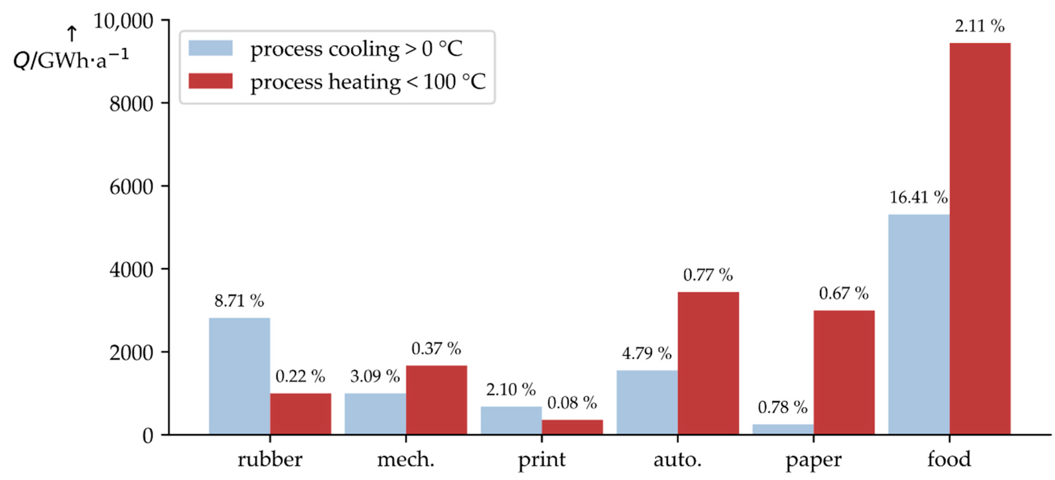
The application of heat pumps in thermal generation circuits in industrial sites is limited because of their temperature range. Heat pumps in industrial applications can generate temperatures up to 100 °C if the heat source provides a sufficient temperature (higher temperatures are possible) [4] (p. 27). The temperature level depends on the industrial application, and therefore, heat pump operation should focus on industries requiring temperature levels below 100 °C. As Figure 1 shows, potential industries include plastics and rubber, mechanical engineering, publication and printing, automotive, paper, and food as they require not only process heating below 100 °C but process cooling with temperatures over 0 °C, which can be provided by heat pump technology [7] (p. 53). The parallel provision of process heating and cooling enables the heat pump to unleash its full potential, which could result in a 30,532 GWh·a⁻¹ annual energy provision by heat pump operation [8] (pp. 82–83) [9] (p. 6). Figure 1 displays the energy percentage that operates below 100 °C (for heating) or over 0 °C (for cooling) according to the industry, for example, 8.71% of the total process cooling demand are over 0 °C and are consumed in the rubber industry [8] (pp. 82–83) [9] (p. 6). Despite these promising numbers, few companies presently leverage the potential of heat pumps. The potential even increases if cooling energy for air conditioning is explored as well. One of the main reasons for this unused potential is the complexity of heat pump integration, especially when both heating and cooling are part of the integration process.

1.3. Methods for Optimal Integration of Heat Pumps

Currently, optimization techniques such as mixed-integer linear programming (MILP) are used to support planners in the heat pump integration process [10,11]. Such algorithms require several simplifications in the modeling of a heat pump and often do not consider design, control, and partial load behavior in combination [12,13,14,15]. Instead of focusing on the simultaneous supply of heating and cooling, only one of them is considered [12,13,14,15]. Therefore, this research addresses the design and control of a heat pump in one MILP algorithm, including state-of-the-art technology (partial load) [16], and simultaneous heating and cooling supply.

In conclusion, a tool was developed to help industrial companies to decarbonize their process heating and cooling supply. The tool calculates the optimal design and operation of heat pumps to integrate them into a thermohydraulic network. The tool is based on a MILP model, which designs the optimal constellation and operation of heat pumps, stratified thermal storage tanks, and a conventional energy converter. The optimization aims to maximize the net present value (NPV), considering an operation period of one year.

The MILP model is elaborated in Section 2. Section 3 validates the MILP model with a sensitivity analysis followed by a comparison with a simulation model, to accurately render the performance of the MILP model [17] (p. 32). In the final section, experiences and limitations of the approach are discussed and concluded.

2. Materials and Methods

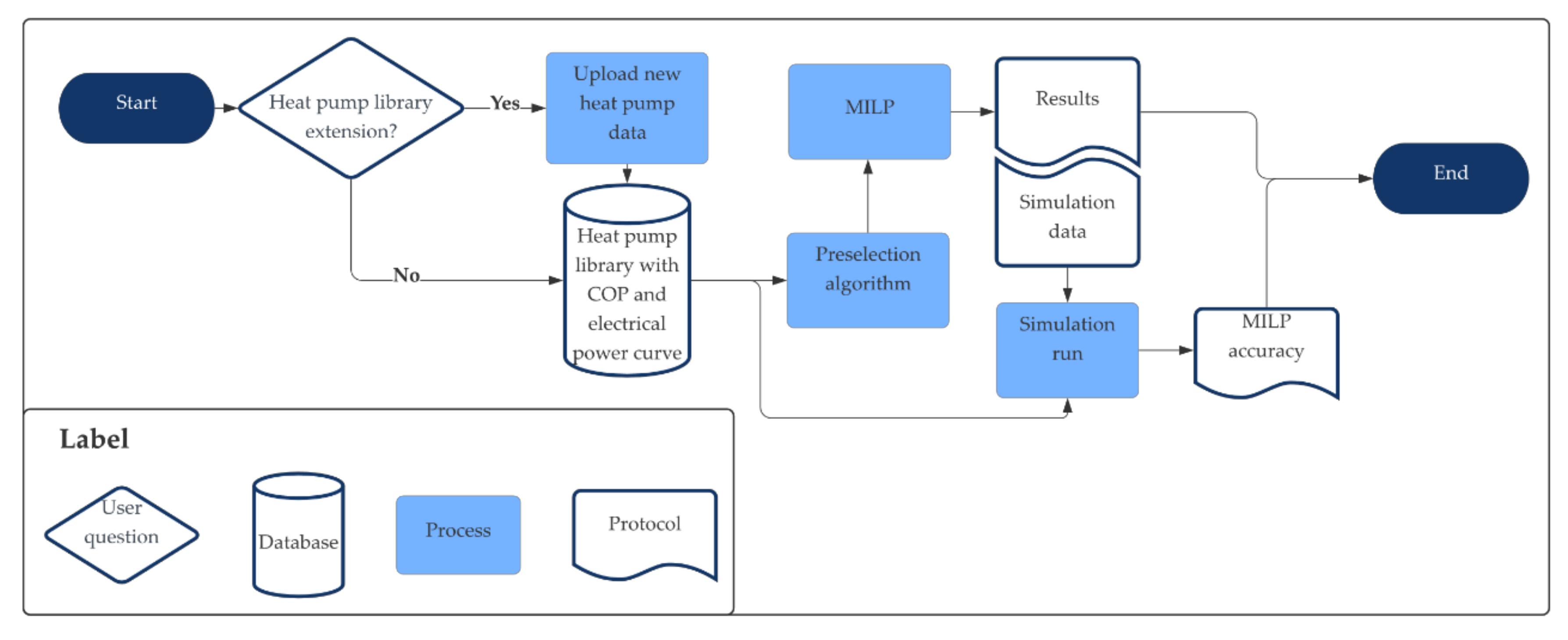
The planning process for the optimal integration of heat pumps is divided into four steps, displayed in Figure 2. In the first step, a potential library for heat pumps is extended by uploading new heat pump models. The optimization model uses this library, as only existing heat pumps should be considered. The library contains heat pump data in terms of the efficiency curve and electrical power curve. The library is then passed to a preselection algorithm to reduce the computational time of the optimization model. In the third step, the optimization model calculates the optimum constellation of heat pumps and stratified thermal storage tanks for a heating and cooling network to meet respective demand within the optimized operation of one year. The optimization model is formulated as a mathematical model from the problem class MILP consisting of a goal function, a solution space as well as decision variables. As MILP representation, the boundary conditions are formulated linearly while the decision variables can also consist of integer variables. The boundary conditions (here the thermohydraulic system) limit the solution space. The optimization computes the minimum or maximum of the objective function [11]. The last step is the optional comparison of the MILP results with a simulation model. The simulation model displays the MILP model in the modeling and simulation environment Dymola and is directly connected with the results from the MILP model through a functional mock-up interface (FMI) [18,19]. The MILP results are then passed to the user in an Excel sheet containing the configuration of heat pumps and stratified thermal storage tanks as well as their operations at each time step (on/off, heat/cold flow rate).

2.1. Mathematical Model

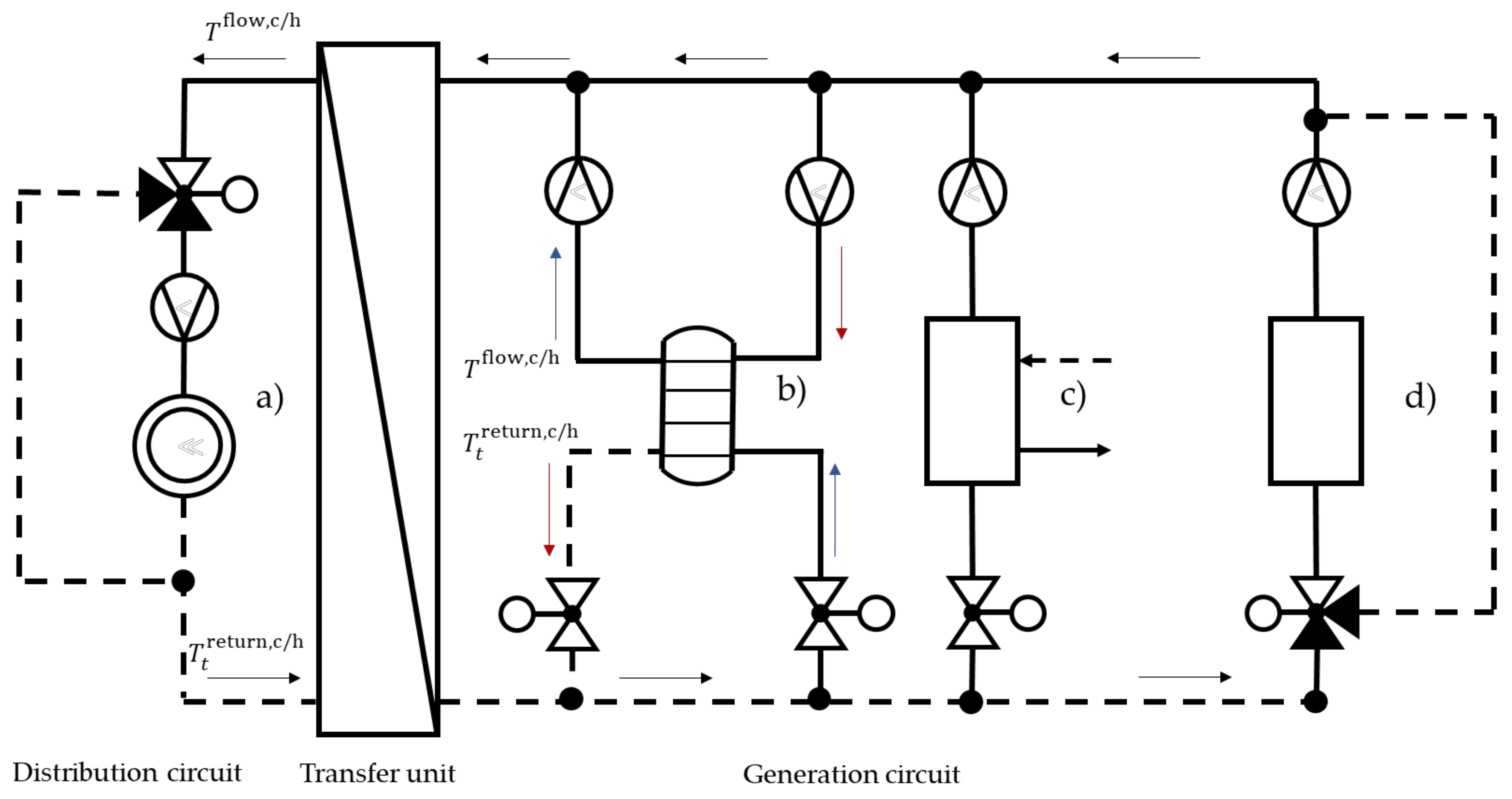
Figure 3 displays a thermohydraulic equivalent circuit of a heating network consisting of a generator circuit (right), a transfer unit (middle), and a distribution circuit (left). Thermal energy is generated by a heat pump (c) and a conventional energy converter (d). The heat pump is connected to a heat source (in this case a cooling network). To offer the heat pump flexibility on the generation side, a stratified thermal storage tank (later referred to as storage) (b) is installed. During the loading process of the storage, a heat rate flows from the flow to the return through the storage layers while the unloading process operates vice versa. The generated energy is transferred through a heat exchanger to the consumer (a).

A MILP model is developed to depict the four components (heat pump, storage, conventional energy converter, consumer) mathematically. All mathematical expressions can be viewed in

Table A5. Symbols (own representation).

Symbol	Unit	Description
$am$	-	amount of purchases of the same heat pump model
$A$	a	payback period
$b_i$	-	binary buying option of heat pump i chosen by optimizer
$c$	J·(kgK)−1	specific heat capacity of water
$c^{\mathrm{c}}$	€·kWh−1	specific costs for cooling energy
$c^{\mathrm{el}}$	€·kWh−1	specific costs for electricity
$c^{\mathrm{h}}$	€·kWh−1	specific costs for heating energy
$c^{\mathrm{st}}$	€·m−3	specific volume price for stratified thermal storage tank
$C_i^{\mathrm{HP}}$	€	price for heat pump i
$C^{\mathrm{tot},\mathrm{opti}}$	€	NPV of optimization (objective function value) chosen by optimizer
$C^{\mathrm{tot},\mathrm{sim}}$	€	NPV of simulation (objective function value)
$CO{P}_{i,t}$	-	COP of heat pump i at time step t
$CO{P}_i^{\mathrm{av}}$	-	averaged COP of heat pump i
$CO{P}_{}^{\mathrm{prep}}$	-	constant COP for preselection algorithm
$E_t^{\mathrm{c}/\mathrm{h}}$	kJ	SOC of the storage (hot/cold) at time step t chosen by optimizer
$Er$	-	error between simulation ($C^{\mathrm{tot},\mathrm{sim}}$) and optimization ($C^{\mathrm{tot},\mathrm{opti}}$)
$i$	-	heat pump
$\Delta m$	kg·s−1	mass flow rate for loading and unloading the storage
$ms$	-	heat pump models
$M$	-	Big-M-Coefficient
$n$	-	number of heat pumps
$P_{i,t}$	kW	electrical power of heat pump i at time step t chosen by optimizer
$P_{i,t}^{\max }$	kW	max. electrical power of heat pump i at time step t
$P_i^{\min }$	kW	min. electrical power of heat pump i
$P_{i,t}^{\mathrm{sim}}$	kW	electrical power of heat pump i at time step t in the simulation
${\dot{Q}}_{}^{}$	kW	heat/cold flow rate
${\dot{Q}}_t^{\mathrm{cd}/\mathrm{hd}}$	kW	heating/cooling demand at time step t
${\dot{Q}}_t^{\mathrm{con},\mathrm{c}/\mathrm{h}}$	kW	conv. heat/cold flow rate at time step t chosen by optimizer
${\dot{Q}}_t^{\mathrm{sim},\mathrm{con},\frac{\mathrm{c}}{\mathrm{h}}}$	kW	conv. heat/cold flow rate at each time step t in the simulation
${\dot{Q}}_{i,t}^{\mathrm{HP},\mathrm{c}/\mathrm{h}}$	kW	heat/cold flow rate of heat pump i at time step t chosen by optimizer
${\dot{Q}}_{}^{\mathrm{nom},\mathrm{h}}$	kW	nominal heat flow rate of heat pump
$S_t^{\mathrm{in}/\mathrm{out},\mathrm{c}/\mathrm{h}}$	kW	heat/cold flow rate for storage loading/unloading at time step t chosen by optimizer
$t$	-	time step of optimization
$\Delta t$	-	time step length
$T_{}^{\mathrm{flow},\mathrm{c}/\mathrm{h}}$	K	cold/hot flow temperature
$T^{\min }$	min	minimum runtime of heat pump
$T_t^{\mathrm{return},\mathrm{c}/\mathrm{h}}$	K	cold/hot return temperature at time step t
$u_{i,t}$	-	binary variable for on-/off-switch of heat pump i at time step t chosen by optimizer
$V_{}^{\mathrm{st},\mathrm{c}/\mathrm{h}}$	m3	cold/hot water storage volume chosen by optimizer
${\vartheta }_t$	-	binary variable to forbid bidirectional flow chosen by optimizer
${\mu }^{\frac{\mathrm{in}}{\mathrm{out}}}$	-	loading/unloading efficiency
$\rho$	kg·m−3	density of the fluid (water)
$\tau$	-	number of time steps
${\tau }_{}^{\mathrm{p}}$	h	operating hours
$\omega$	-	energy efficiency of the storage from time step $t-1$ to $t$

. The model integrates storages and heat pumps into an existing thermohydraulic network consisting of a distribution circuit, transfer unit, and generation circuit with a conventional energy converter. The thermohydraulic equivalent circuit represents the heating and cooling networks, which are modeled analogously to each other. The major assumption of the model is that all energy converters and the storage feed into the network with the same temperature $T_{}^{\mathrm{flow},\mathrm{c}/\mathrm{h}}$ and receive the same return temperature $T_t^{\mathrm{return},\mathrm{c}/\mathrm{h}}$ from the transfer unit (heat exchanger). However, the storage feed into the flow strand could be lower than $T_{}^{\mathrm{flow},\mathrm{c}/\mathrm{h}}$ if all layers do not have the flow temperature. This results in a mixing temperature lower than the required demand temperature.

The MILP model seeks the most cost-efficient configuration of heat pumps and flexibility options (storages). The cost-efficient objective is achieved by optimizing the operation of the generation circuit to meet the demand over one year with a temporal resolution of $\Delta t$. The objective function is modeled after the NPV method [20] (p. 24). The costs are divided into capital expenditures (capex) and operational expenditures (opex). The capex consist of the sum of all heat pump prices $C_i^{\mathrm{HP}}$ with the buying option $b_i$ and the storage prices (hot and cold water storage), which are calculated with a volume-specific price of $c^{\mathrm{st}}$ and the storage dimension ($V_{}^{\mathrm{st},\mathrm{c}/\mathrm{h}}$). The capex do not include investments for conventional energy converters that are assumed to have been integrated into the thermohydraulic network previously. Meanwhile, opex are divided into unoptimized opex and optimized opex. The optimized opex consist of heat pump costs $c^{\mathrm{el}}$ for electric power P_i,t, costs for conventional heating $c^{\mathrm{h}}$ with a heat flow rate ${\dot{Q}}_t^{\mathrm{con},\mathrm{h}}$, and costs for conventional cooling $c^{\mathrm{c}}$ with a cold flow rate ${\dot{Q}}_t^{\mathrm{con},\mathrm{c}}$. The unoptimized opex are the operational cost of meeting the heating and cooling demand ${\dot{Q}}_t^{\mathrm{con},\mathrm{c}/\mathrm{h}}$ with conventional heating and cooling. The profit is calculated by subtracting the optimized opex from the unoptimized opex. The profit is discounted over a payback period $A$ with an interest rate $z$. To achieve the most cost-efficient configuration, the objective function $C^{\mathrm{tot},\mathrm{opti}}$ must be maximized:

$$\begin{gathered} \max C^{\mathrm{tot},\mathrm{opti}}=-\left[\left({\displaystyle \sum }_{i=1}^n(C_i^{\mathrm{HP}}\times b_i)\right)+c^{\mathrm{st}}\times \left(V_{}^{\mathrm{st},\mathrm{c}}+V_{}^{\mathrm{st},\mathrm{h}}\right)\right] \\ +\Delta t\times \left[c^{\mathrm{c}}\times {\displaystyle \sum }_{t=1}^{\tau }{\dot{Q}}_t^{\mathrm{cd}}+c^{\mathrm{h}}\times {\displaystyle \sum }_{t=1}^{\tau }{\dot{Q}}_t^{\mathrm{hd}}-c^{\mathrm{c}}\times {\displaystyle \sum }_{t=1}^{\tau }{\dot{Q}}_t^{\mathrm{con},\mathrm{c}}-c^{\mathrm{h}}\times {\displaystyle \sum }_{t=1}^{\tau }{\dot{Q}}_t^{\mathrm{con},\mathrm{h}}-c^{\mathrm{el}}\times {\displaystyle \sum }_{i=1}^n{\displaystyle \sum }_{t=1}^{\tau }{P}_{i,t}\right] \\ \times \frac{{\left(1+z\right)}^A-1}{{\left(1+z\right)}^A\times z}. \end{gathered}$$

(1)

The satisfaction of heating or cooling demand ${\dot{Q}}_t^{\mathrm{cd}/\mathrm{hd}}$ is ensured by the following condition:

$${\dot{Q}}_t^{\mathrm{cd}/\mathrm{hd}}={\displaystyle \sum }_{i=1}^n{\dot{Q}}_{i,t}^{\mathrm{HP},\mathrm{c}/\mathrm{h}}+S_t^{\mathrm{out},\mathrm{c}/\mathrm{h}}-S_t^{\mathrm{in},\mathrm{c}/\mathrm{h}}+{\dot{Q}}_t^{\mathrm{con},\mathrm{c}/\mathrm{h}} \forall i=1, \dots ,n,\forall t=1,\dots ,\tau ,$$

(2)

where $S_t^{\mathrm{out},\mathrm{c}/\mathrm{h}}$ is the heat/cold flow rate out of the storage, $S_t^{\mathrm{in},\mathrm{c}/\mathrm{h}}$ is the heat/cold flow rate into the storage, and ${\dot{Q}}_{i,t}^{\mathrm{HP},\mathrm{c}/\mathrm{h}}$ is the heat/cold flow rate for every heat pump.

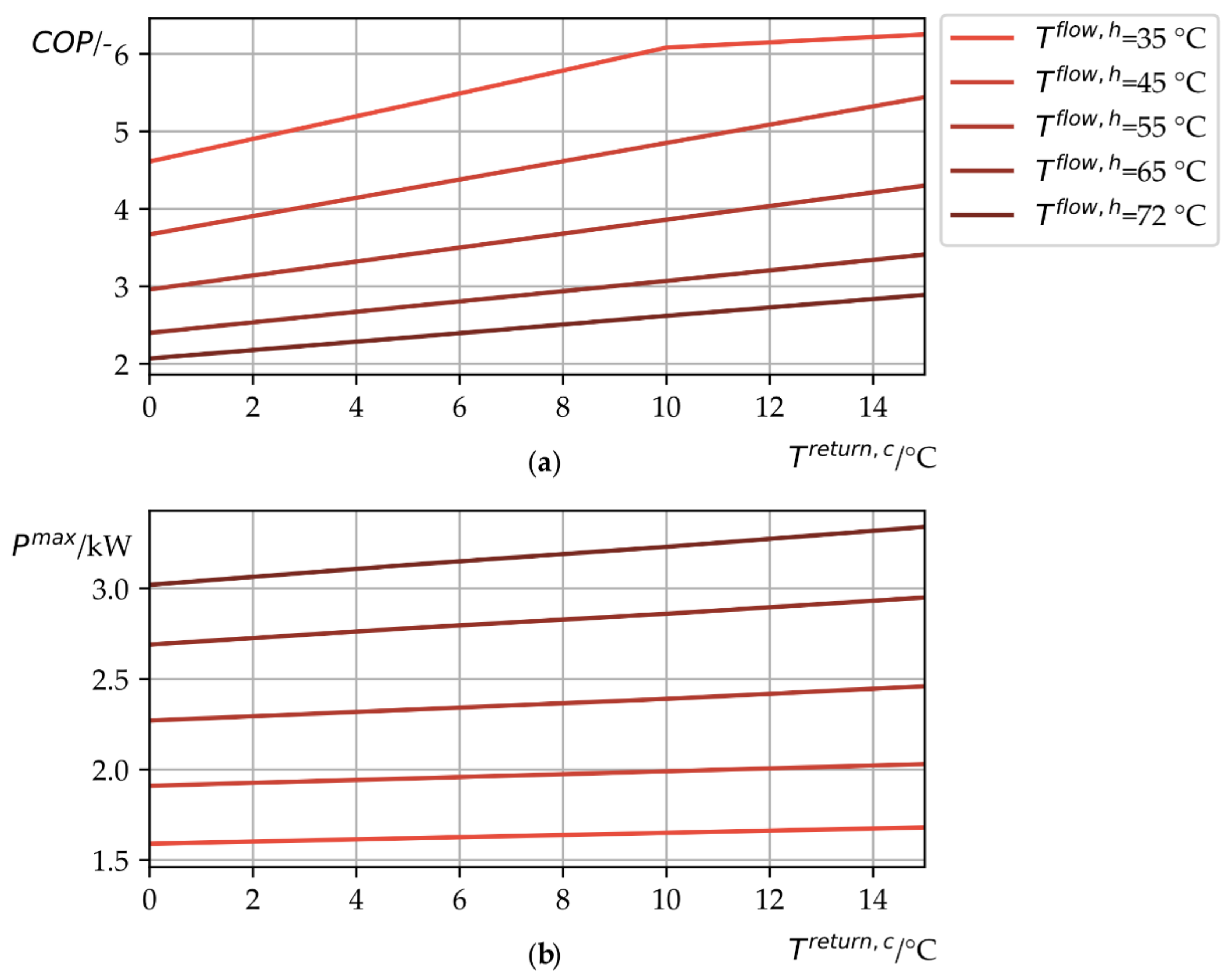
The heat pump is modeled as a quasi-stationary process, and its heat/cold flow rate is calculated with the coefficient of performance (COP) [21] (pp. 312–314). It is assumed that the temperatures of the network do not change with the integration of the heat pumps and, therefore, are given (assumption is checked in Section 3.3). The COP and the electrical power curve are then linearized with a multiple linear regression [22] (pp. 51–53). An example data sheet is provided in Appendix A (Figure A1). The COP and the maximum electrical power depend on the flow temperature in the heating circuit and the return temperature in the cooling circuit [7]. These temperatures are assumed to be given in 15 min time steps over one year. With the regressor functions for every heat pump and the given temperatures at each time step, the $CO{P}_{i,t}$, the maximum electrical power $P_{i,t}^{\max }$, and the minimum electrical power $P_i^{\min }$ (time independent) can be calculated for one year production prior to the optimization. This results in the linear calculation of the heat flow rate ${\dot{Q}}_{i,t}^{\mathrm{HP},\mathrm{h}}$ for every heat pump i at each time step t [21] (pp. 312–314):

$${\dot{Q}}_{i,t}^{\mathrm{HP},\mathrm{h}}=P_{i,t}\times CO{P}_{i,t} i=1, \dots ,n,\forall t=1,\dots ,\tau .$$

(3)

The electrical power $P_{i,t}$ of a heat pump, $i$, can be chosen by the optimizer and is limited by the regressor function for the maximum electrical power $P_{i,t}^{\max }$ and minimum electrical power $P_i^{\min }$ of the heat pump $i$, with

$$u_{i,t}\times P_i^{\min }\le P_{i,t}\le u_{i,t}\times P_{i,t}^{\max } \forall i=1, \dots ,n,\forall t=1,\dots ,\tau ,$$

(4)

$$P_{i,t}\le b_i\times P_{i,t}^{\max } \forall i=1, \dots ,n,\forall t=1,\dots ,\tau ,$$

(5)

where $b_i$ in Equation (5) is the binary buying option and where $u_{i,t}$ in Equation (4) is the binary on-/off-switch for the heat pump. Equation (4) gives the optimizer the flexibility option of partial load by choosing $P_{i,t}$ between the maximum and minimum electrical power feed into the heat pump. The cold flow rate ${\dot{Q}}_{i,t}^{\mathrm{HP},\mathrm{c}}$ is calculated analogically to Equation (3) with [23]:

$${\dot{Q}}_{i,t}^{\mathrm{HP},\mathrm{c}}=P_{i,t}\times (CO{P}_{i,t}-1) \forall i=1, \dots ,n,\forall t=1,\dots ,\tau .$$

(6)

Every heat pump can be turned on and off to offer the optimizer another flexibility option with the binary variable $u_{i,t}$. The power circuit of a heat pump should not be interrupted too frequently; therefore, a minimum runtime $T^{\min }$ is ensured with the following:

$$T^{\min }\times \left(u_{i,t}-u_{i,\left(t-1\right)}\right)\le {\displaystyle \sum }_{t^{\prime }=1}^{T^{\min }-1}{u}_{i,t^{’}} \forall i=1, \dots ,n,\forall t=1,\dots ,\tau -T^{\min }-1,$$

(7)

The most important element of flexibility in the MILP model is related to storage. The optimizer can choose its dimension freely and is limited only by the space $V^{\max }$ that the user can offer for hot and cold water storages ($V_{}^{\mathrm{st},\mathrm{h}}, V_{}^{\mathrm{st},\mathrm{c}}$):

$$0\le V_{}^{\mathrm{st},\mathrm{h}}+V_{}^{\mathrm{st},\mathrm{c}}\le V^{\max }.$$

(8)

The storage loading (marked as a red arrow) and unloading (marked as a blue arrow) in Figure 3 are modeled as the power flow of an electric battery:

$$E_t^{\mathrm{c}/\mathrm{h}}=\omega \times E_{t-1}^{\mathrm{c}/\mathrm{h}}+\Delta t\times \left({\mu }^{\mathrm{in}}\times S_t^{\mathrm{in},c/h}-\frac{1}{{\mu }^{\mathrm{out}}}\times S_t^{\mathrm{out},c/h}\right) \forall t=2,\dots ,\tau .$$

(9)

The current state of charge (SOC) is $E_t^{\mathrm{c}/\mathrm{w}}$ (current energy level). It is calculated by the sum of SOC from time step $t-1$ and the heat/cold flow rate $S_t^{\mathrm{in},\mathrm{c}/\mathrm{h}}$ to load the storage over a time step length $\Delta t$. The heat/cold flow rate $S_t^{\mathrm{out},\mathrm{c}/\mathrm{h}}$ to unload the storage over a time step length $\Delta t$ is subtracted. The efficiencies for loading and unloading the storage are expressed by ${\mu }^{\mathrm{in}}$ and ${\mu }^{\mathrm{out}}$. The energy losses of the storage from time step $t-1$ to $t$ are expressed by multiplying $E_t^{\mathrm{c}/\mathrm{w}}$ with an efficiency $\omega$. The energy level of the storage is limited by the current return temperature $T_t^{\mathrm{return},\mathrm{c}/\mathrm{h}}$ and the constant flow temperature $T_{}^{\mathrm{flow},\mathrm{c}/\mathrm{h}}$:

$$0\le E_t^{\mathrm{h}}\le c\times V_{}^{\mathrm{st},\mathrm{h}}\times \rho \times \left(T_{}^{\mathrm{flow},\mathrm{h}}-T_t^{\mathrm{return},\mathrm{h}}\right) \forall t=1,\dots ,\tau ,$$

(10)

$$0\le E_t^{\mathrm{c}}\le c\times V_{}^{\mathrm{st},\mathrm{c}}\times \rho \times \left(T_t^{\mathrm{return},\mathrm{c}}-T_{}^{\mathrm{flow},\mathrm{c}}\right) \forall t=1,\dots ,\tau ,$$

(11)

where $\rho$ is the density of water and where $c$ is the specific heat capacity of water. The storage is modeled as stratified storage, and these equations follow the assumption that the energy level of the storage is equal to zero if all layers have the return temperature $T_t^{\mathrm{return},\mathrm{c}/\mathrm{h}}$. The energy level of the storage is at its maximum if all layers have the flow temperature $T_{}^{\mathrm{flow},\mathrm{c}/\mathrm{h}}$. Furthermore, it is assumed that the storage unloads and loads always with the flow temperature $T_{}^{\mathrm{flow},\mathrm{c}/\mathrm{h}}$. The unloading and loading process is limited according to the following:

$$0\le S_t^{\mathrm{in}/\mathrm{o}ut,\mathrm{c}/\mathrm{h}}\le \Delta m\times c\times \left(T_{}^{\mathrm{flow},\mathrm{h}}-T_t^{\mathrm{return},\mathrm{h}}\right) \forall t=1,\dots ,\tau ,$$

(12)

$$0\le S_t^{\mathrm{in}/\mathrm{o}ut,\mathrm{c}/\mathrm{h}}\le \Delta m\times c\times \left(T_t^{\mathrm{return},\mathrm{c}}-T_{}^{\mathrm{flow},\mathrm{c}}\right) \forall t=1,\dots ,\tau ,$$

(13)

where $\Delta m$ is the mass flow rate to load or unload the storage. To ensure stable flow conditions during the loading and unloading process, bidirectional flow is forbidden:

$$S_t^{\mathrm{in},\mathrm{c}/\mathrm{h}}\le {\vartheta }_t\times M \forall t=1,\dots ,\tau ,$$

(14)

$$S_t^{\mathrm{o}ut,\mathrm{c}/\mathrm{h}}\le \left(1-{\vartheta }_t\right)\times M \forall t=1,\dots ,\tau ,$$

(15)

where ${\vartheta }_t$ is a binary variable and $M$ is a Big-M-Coefficient [11] (p. 219). The binary variable ensures that during the loading process $S_t^{\mathrm{o}ut,\mathrm{c}/\mathrm{h}}$ will be equal to zero because ${\vartheta }_t$ will be one: $\left(1-1\right) · M=0$. During the unloading process ${\vartheta }_t$ will be equal to zero to forbid loading the storage: $0·M=0$. For the Big-M-Coefficient applies $M\gg S_t^{\mathrm{in},\mathrm{c}/\mathrm{h}}$ and $M\gg S_t^{\mathrm{out},\mathrm{c}/\mathrm{h}}$, therefore, the loading and unloading process is only limited by Equations (12) and (13).

In addition to the mathematical formulation, it should be noted that all parameters (technical or economic) can be easily changed (e.g., efficiencies, fluid parameters). Although the heat pump library is static, it can also be modified by the user. The model can select from all available heat pumps, which results in an exponential rise of the computational time, and therefore, an algorithm is developed to reduce computational time by preselecting possible options.

2.2. Preselection Algorithm

The preselection algorithm consists of a power limit through the nominal heat output and an efficiency comparison. The assumed spread between the cooling and heating demands in the industry is typically quite large, where ${\dot{Q}}_t^{\mathrm{cd}}\ll {\dot{Q}}_t^{\mathrm{hd}}$, which means that the cooling demand would be the limiting factor of the heat pump operation [24]. That said, the nominal heat output ${\dot{Q}}_{}^{\mathrm{nom},\mathrm{h}}$ of a heat pump with a constant $CO{P}_{}^{\mathrm{prep}}$ is limited by the cumulative cooling demand $Q_{}^{\mathrm{cd}}$ over the period ${\tau }_{}^{\mathrm{p}}$ with [4] (p. 54):

$${\dot{Q}}_{}^{\mathrm{nom},\mathrm{h}}\le \frac{Q_{}^{\mathrm{cd}}}{{\tau }_{}^{\mathrm{p}}}\times \frac{CO{P}_{}^{\mathrm{prep}}}{CO{P}_{}^{\mathrm{prep}}-1}.$$

(16)

In addition to the power limit of the heat pump, the algorithm calculates the average $CO{P}_i^{\mathrm{av}}$ for every heat pump $i$ depending on the given temperatures $T_t^{\mathrm{return},\mathrm{c}/\mathrm{h}}$ and $T_{}^{\mathrm{flow},\mathrm{c}/\mathrm{h}}$. Then, a defined number of heat pump models with the highest $CO{P}_i^{\mathrm{av}}$ are selected. The algorithm preselects certain heat pump models ($ms$) and limits their amount ($am$) of purchases of the same heat pump model. These parameters can be modified and significantly change computational time.

2.3. Simulation Model

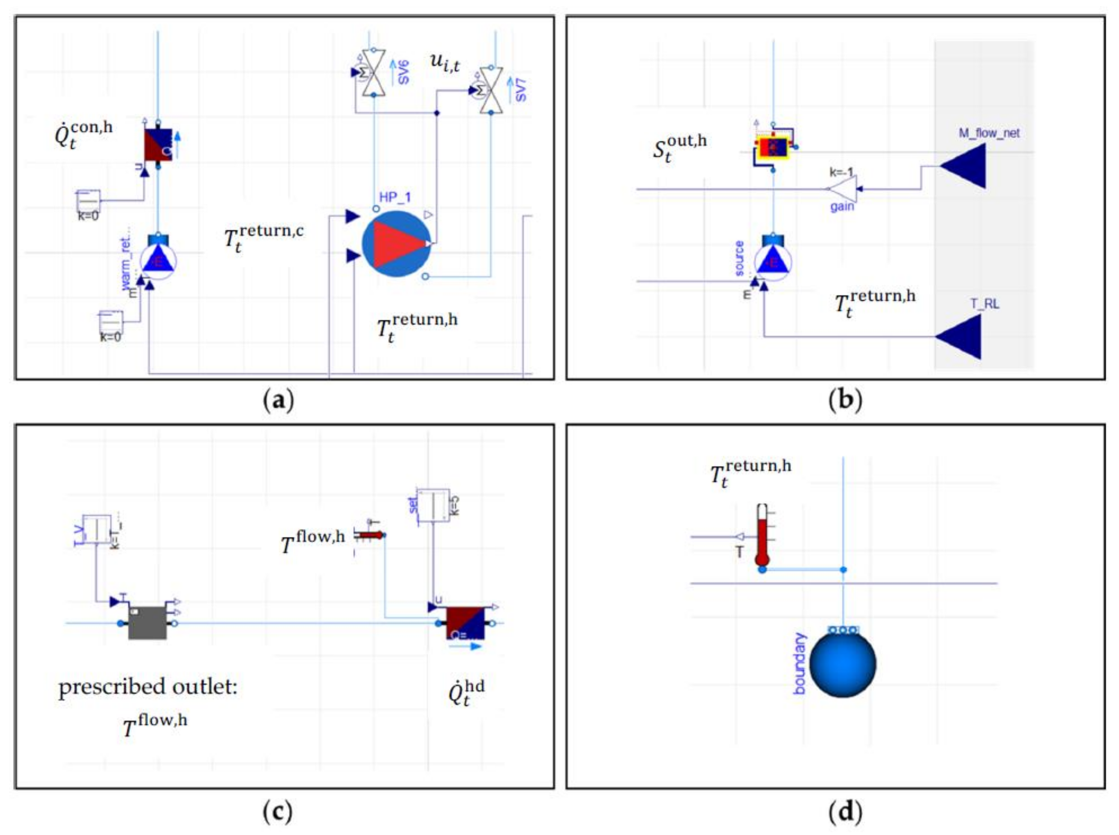
A simulation model was developed for validation purposes (see Figure 4).

The model was developed in the Modelica modeling language using the libraries: “ModelicaStandardLibrary” and “Buildings” [25]. The generator circuit receives a signal with the current return temperature from the boundary block in Figure 4d (“Modelica.Fluid.Sources.FixedBoundary”). The return strand is modeled by a source block (see Figure 4b—“Modelica.Fluid.Sources.MassFlowSource_T”), which feeds into the generators with the corresponding return temperature. The respective mass flow rate is calculated for each generator based on the MILP results ($S_t^{\mathrm{in}/\mathrm{o}ut,\mathrm{c}/\mathrm{h}}$, ${\dot{Q}}_t^{\mathrm{HP},\mathrm{c}/\mathrm{h}}$, ${\dot{Q}}_t^{\mathrm{con},\mathrm{c}/\mathrm{h}}$). The energy converter is modeled by a heating/cooling block (see Figure 4a—“Buildings.Fluid.HeatExchangers.HeaterCooler_u”) and receives a signal u of the current heat flow rate ${\dot{Q}}_t^{\mathrm{con},\mathrm{c}/\mathrm{h}}$. The heat pumps’ and storages’ inflow is controlled by a valve (SV6 or SV7 in Figure 4a—“Modelica.Fluid.ValvesIncompressible”). The storage is modeled as stratified storage (see Figure 4b—“Buildings.Fluid.Storage.Stratified”). The heat pumps (HP_1) cooling component is modeled by a heating/cooling block as well (“Buildings. Fluid.HeatExchangers.HeaterCooler_u”). It receives a signal of the current cold flow rate calculated by the COP and the electrical power, which are based on the regressor function from the MILP model and have the cold return temperature of every simulation step and the hot flow temperature as an input. A heating block (“Buildings. Fluid.HeatExchangers. Heater_T”) receives the electrical power, the COP, the maximum heat flow rate, and the needed heat flow temperature as inputs. The output of this block is the actual heat flow rate, which is needed to calculate the electrical power for the NPV $C^{\mathrm{tot},\mathrm{sim}}$. Before the fluid flows into the consumer, its temperature is adjusted to the prescribed flow temperature $T_{}^{\mathrm{flow},\mathrm{c}/\mathrm{h}}$ with the first block in Figure 4c (“Buildings. Fluid.HeatExchangers.PrescribedOutlet”). The consumer is modeled with a heating/cooling block (“Buildings. Fluid.HeatExchangers.HeaterCooler_u”), and it receives the current demand ${\dot{Q}}_t^{\mathrm{cd}/\mathrm{hd}}$. Afterward, the fluid flows into the boundary block.

The results of the MILP model are necessary inputs for the simulation model. The simulation model requires information about the heat pump constellation ($b_i$) (heat pump model and purchase amount) and the storage size for the heating and cooling network, if needed. The operation signals of every energy converter in the generation circuit (including the storages) and the distribution circuit are passed to the simulation model as well. In conclusion, the following results and parameters are given to the simulation:

• flow temperatures $T_{}^{\mathrm{flow},\mathrm{c}/\mathrm{h}}$ to adjust the heat pump operation,
• regression function to calculate the $CO{P}_{it}$ and the maximum electrical power $P_{i,t}^{\max }$ for the heat pump operation in the simulation with the simulation’s return temperature and the passed flow temperature $T_{}^{\mathrm{flow},\mathrm{c}/\mathrm{h}}$,
• minimum electrical power $P_i^{\min }$ to limit the heat pumps’ operation in the simulation,
• time step $\Delta t$ to adjust the time series in the simulation,
• buying decision $b_i$ to implement the heat pump constellation into the simulation,
• storage volumes $V_{}^{\mathrm{st},\mathrm{c}}$ and $V_{}^{\mathrm{st},\mathrm{h}}$ to pass the dimension into the simulation,
• heating and cooling demand ${\dot{Q}}_t^{\mathrm{cd}/\mathrm{hd}}$ at each time step $t$ to model the consumer in the simulation,
• conventional heating and cooling ${\dot{Q}}_t^{\mathrm{con},\mathrm{c}/\mathrm{h}}$ at each time step $t$ to model a conventional energy converter in the simulation,
• value of the objective function $C^{\mathrm{tot},\mathrm{opti}}$ to insert it into Equation (17),
• heat and cold flow rate ${\dot{Q}}_{i,t}^{\mathrm{HP},\mathrm{c}/\mathrm{h}}$ of every heat pump at each time step to calculate the mass flow rates in the simulation,
• loading and unloading heat flow rate $S_t^{\mathrm{in}/\mathrm{o}ut,\mathrm{c}/\mathrm{h}}$ for the storage to set it in the simulation.

The listing is summarized in

Table A4. A list of passed objects from the optimizer to the simulation and their objective (own representation).

Passed Object	Type of Parameter	Information
regressor function for $CO{P}_{i,t}$ and $P_{i,t}^{\max }$	equation	calculates the $CO{P}_{it}$ and $P_{it}^{\max }$ depending on the temperatures in the simulation
$P_i^{\min }$	initial parameter	limits the electrical power of every heat pump
$\Delta t$	parameter for equation	time information (time step length)
$b_i$	initial parameter	purchased heat pumps to be installed in the simulation
$V_{}^{\mathrm{st},\mathrm{c}/\mathrm{h}}$	initial parameter	dimension of the storages in the simulation
${\dot{Q}}_t^{\mathrm{cd}/\mathrm{hd}}$	time-dependent parameter	heating and cooling demand for the simulation
${\dot{Q}}_t^{\mathrm{con},\mathrm{c}/\mathrm{h}}$	time-dependent parameter	conventional heating and cooling at each time step for the simulation
$T_{}^{\mathrm{flow},\mathrm{c}/\mathrm{h}}$	initial parameter	flow temperatures are set before the simulation start
$C^{\mathrm{tot},\mathrm{opti}}$	initial parameter	value of the objective function for comparison
$S_t^{\mathrm{in}/\mathrm{o}ut,\mathrm{c}/\mathrm{h}}$	time-dependent parameter	storage loading and unloading at each time step for the simulation
${\dot{Q}}_t^{\mathrm{HP},\mathrm{c}/\mathrm{h}}$	time-dependent parameter	heat/cold flow rate to calculate mass flow rates for every heat pump at each time step

. The COP and the electrical power input of every heat pump are recalculated in each time step based on the resulting temperatures in the simulation (see regressor function in Table A4). The heat and cold flow rates of the heat pumps in the simulation model are calculated in analogy with the mathematical model; however, the simulation has a much sharper resolution of 60 s time steps. In the simulation model, the fluid in front of the consumer is forced to emerge with the flow temperature $T_{}^{\mathrm{flow},\mathrm{c}/\mathrm{h}}$. In case of incorrect calculations in the mathematical optimization resulting in an incorrect flow temperature, the additional power to lift or lower the fluid’s temperature is added in terms of amount to the conventional energy converter ${\dot{Q}}_t^{\mathrm{sim},\mathrm{con},\mathrm{c}/\mathrm{h}}$. After the simulation is finished, the new values for electrical power $P_{i,t}^{\mathrm{sim}}$ and conventional heating/cooling ${\dot{Q}}_t^{\mathrm{sim},\mathrm{con},\mathrm{c}/\mathrm{h}}$ are inserted into Equation (1) to calculate the objective function value $C^{\mathrm{tot},\mathrm{sim}}$ for the simulation run. The error $Er$ between the objective values $C^{\mathrm{tot},\mathrm{sim}}$ and $C^{\mathrm{tot},\mathrm{opti}}$ is calculated using the following formula:

$$Er=\frac{\sqrt{{\left(C^{\mathrm{tot},\mathrm{sim}}-C^{\mathrm{tot},\mathrm{opti}}\right)}^2}}{C^{\mathrm{tot},\mathrm{opti}}}\times 100.$$

(17)

3. Results

The presented method and model were applied to an industrial use case. Firstly, a parameter study was conducted to analyze the behavior of the mathematical model. Secondly, the method, including the preselection, mathematical model, and simulation model, was applied. Thus, the results of the MILP model and the simulation model can be compared to evaluate the error $Er$ and proof the temperature assumptions (see Section 2.1).

3.1. Industrial Use Case

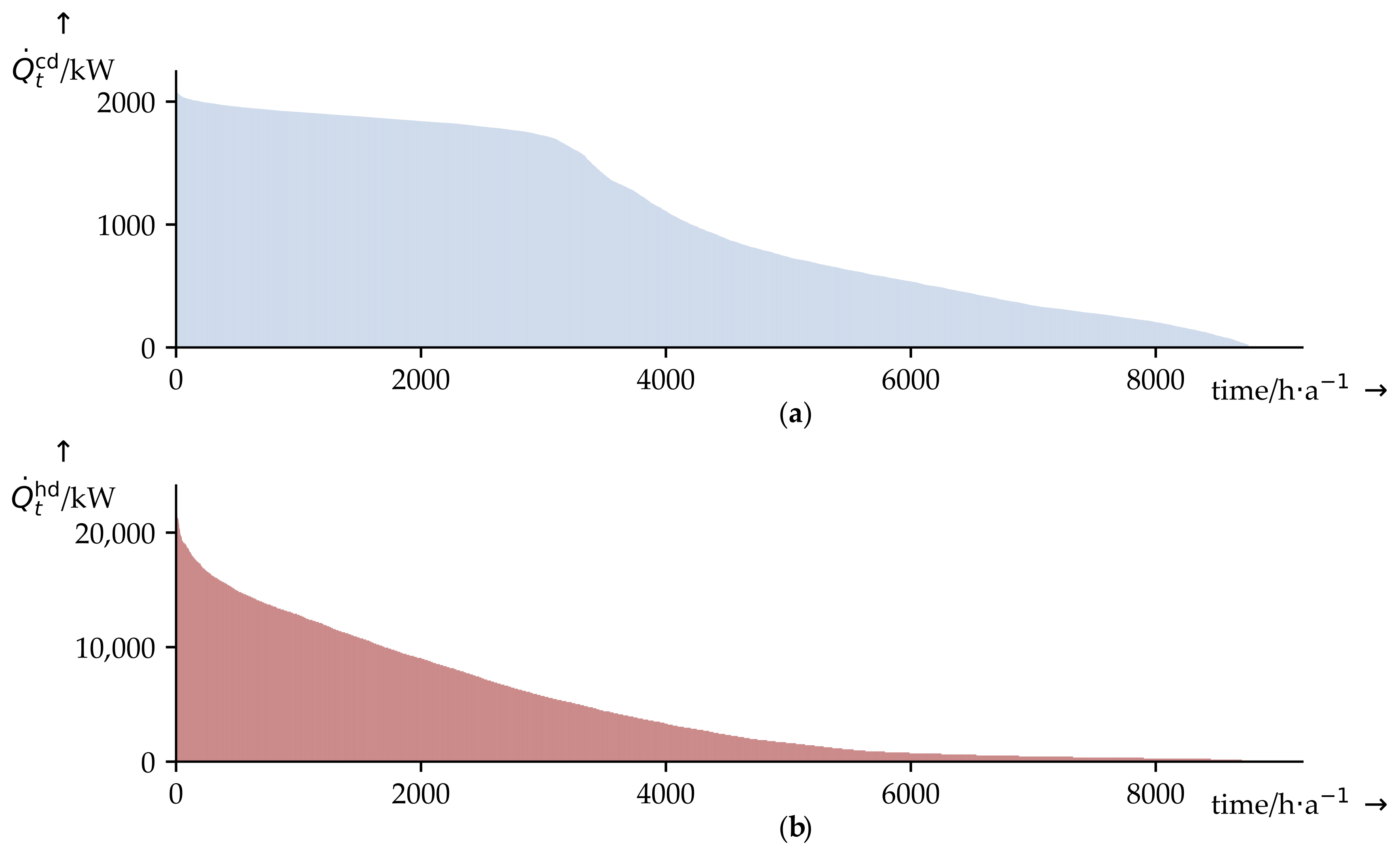
An industrial use case serves as the basis for the sensitivity analysis. Figure 5 displays the cumulative heating (b) and cooling demand (a) of the industrial example. The demands differ by a factor of 10, and the major cooling power operates below 1 MW while the major heating power operates below 3 MW. The heating demand has peaks up to 20 MW while the cooling demand reaches its maximum around 2 MW.

The heat pumps considered for the industrial use case can be found in [7] (pp. 10–14, 23–26, 49–51, 55–57). The power output ($P_{i,t}^{\max }$, $P_i^{\min }$, ${\dot{Q}}_{}^{\mathrm{nom},\mathrm{h}}$) is scaled up by a factor of 10 to adapt the heat pumps to the demand of industrial example. The scale up has no influence on the heat pumps’ temperature range according to their datasheet, and its purpose is the proper analysis.

Table 1. Heat pump library [7].

Heat Pump	${\dot{\mathit{Q}}}_{}^{\mathbf{nom},\mathbf{h}}/\mathbf{kW}$	${\mathit{C}}_{\mathit{i}}^{\mathbf{HP}}/€$	Heat Pump	${\dot{\mathit{Q}}}_{}^{\mathbf{nom},\mathbf{h}}/\mathbf{kW}$	${\mathit{C}}_{\mathit{i}}^{\mathbf{HP}}/€$
BWC 201 A06	57.6	18,642.24	BW 301 A08	103.6	24,166.07
BWC 201 A08	76.3	21,109.58	BW 301 A10	134	27,077.49
BWC 201 A10	97.4	23,515.66	BW 301 A13	171.3	30,182.80
BWC 201 A13	130	26,717.13	BW 351 A07	73.5	20,763.52
BWC 201 A17	172	30,237.27	BW 351 A18	186.5	31,338.81
BWT 221 A06	59	18,841.22	BWC 351 A07	73.3	20,738.53
BWT 221 A08	77	21,194.98	BW 301 A06	78.6	21,388.57
BWT 221 A10	100	23,791.15

displays all heat pumps in the library with their scaled values for the nominal heat flow rate and their respective price depending on ${\dot{Q}}_{}^{\mathrm{nom},\mathrm{h}}$ calculated with an empirical survey from 2012 [4] (p. 24).

3.2. Sensitivity Analysis

The sensitivity analysis is divided into several parameter studies and is performed without the validation of the simulation model (validation follows in Section 3.3).

Table 2. Parameters set before the optimization, referred to as the standard.

Symbol	Value	Symbol	Value
${\tau }^{\mathrm{p}}$	6000 h [4] (p. 54)	$\Delta T_{}^{\max }$	6 K
$CO{P}_{}^{\mathrm{prep}}$	6 [4] (p. 66)	$c^{\mathrm{h}}$	0.04 €·kWh−1
${\dot{m}}_t^{\mathrm{c}}$	85 kg·s−1	$c^{\mathrm{c}}$	0.06 €·kWh−1
${\dot{m}}_t^{\mathrm{h}}$	1000 kg·s−1	$c^{\mathrm{el}}$	0.12 €·kWh−1 [26] (p. 2)
$z$	0.06 [20] (p. 14)	$\Delta t$	60 min
$A$	5 a [27] (p. 5)	$T_{}^{\min }$	60 min [28] (p. 7)
$c^{\mathrm{st}}$	3186.36 €·m−3 [29] (pp. 288–290)	$\alpha$	$\approx$1
$\Delta m$	10 kg·s−1	${\mu }^{\mathrm{in}/\mathrm{o}ut}$	0.98
$c$	4.182 kJ·kg−1·K−1 [30] (p. 97)	$ms$	5
$\rho$	997 kg·m−3 [30] (p. 92)	$am$	8
$T_{}^{\mathrm{flow},\mathrm{h}}$	60 °C	$M$	108
$T_{}^{\mathrm{flow},\mathrm{c}}$	16 °C

presents the input for the MILP model, which serves as a comparative example (standard) for the parameter study. The mass flow rates for the heating and cooling network ${\dot{m}}_t^{\mathrm{c}/\mathrm{h}}$ are calculated using the demand and the given temperatures [21] (pp. 327–328). The maximum temperature spread $\Delta T_{}^{\max }$ between the flow and return temperature is 6 K, and the time step is set to 60 min for the parameter study.

Table 3. Parameter variation for the parameter study (own representation).

Name	Parameter	Variation
1. Standard case	none	none
2. Demand	${\dot{Q}}_t^{\mathrm{hd}}$	80% ${\dot{Q}}_t^{\mathrm{hd}}$, 60% ${\dot{Q}}_t^{\mathrm{hd}},$40% ${\dot{Q}}_t^{\mathrm{hd}}$
	${\dot{Q}}_t^{\mathrm{cd}}$	80% ${\dot{Q}}_t^{\mathrm{cd}},$60% ${\dot{Q}}_t^{\mathrm{cd}},$40% ${\dot{Q}}_t^{\mathrm{cd}}$
	${\dot{Q}}_t^{\mathrm{cd}/\mathrm{hd}}$	80% ${\dot{Q}}_t^{\mathrm{cd}/\mathrm{hd}},$60% ${\dot{Q}}_t^{\mathrm{cd}/\mathrm{hd}},$40% ${\dot{Q}}_t^{\mathrm{cd}/\mathrm{hd}}$
3. Temperature	$T_{}^{\mathrm{flow},\mathrm{c}}$, $T_{}^{\mathrm{flow},\mathrm{h}}$	$T_{}^{\mathrm{flow},\mathrm{c}}$ = 5 °C and $T_{}^{\mathrm{flow},\mathrm{h}}$ = 60 °C $T_{}^{\mathrm{flow},\mathrm{c}}$ = 5 °C and $T_{}^{\mathrm{flow},\mathrm{h}}$ = 66 °C $T_{}^{\mathrm{flow},\mathrm{c}}$ = 5 °C and $T_{}^{\mathrm{flow},\mathrm{h}}$ = 75 °C
4. Costs	$c^{\mathrm{h}}$, $c^{\mathrm{c}}$, $c^{\mathrm{el}}$	$c^{\mathrm{c}}$ = 0.04 €·kWh−1 $c^{\mathrm{h}}$ = 0.02 €·kWh−1 $c^{\mathrm{el}}$ = 0.14 €·kWh−1
5. Storage	$V^{\max }$	$V^{\max }$ = 0
6. Preselection algorithm	$ms$, $am$	$ms$ = 15 and $am$ = 3

displays the parameter variation for the parameter study. Demands are reduced individually and collectively to examine the influence of the respective demand (heating/cooling). Furthermore, temperature changes are investigated to evaluate their influence on efficiency and to understand how the tool reacts. The change in the specific costs should highlight the benefit of the heat pump and how the specific costs differently affect the NPV. The influence of the storage is determined, as well. The variation of the heat pump selection and the buying amount of one model primarily examines the influence of the preselection algorithm. An example of the heat pump selection would be two possible heat pump models ($ms=2$) and each model can be purchased three times ($am=3$).

3.2.1. Standard Case

For comparative reasons, the standard run or reference case of the MILP model (Table 3) is briefly introduced.

Table 4. Results of the standard run (own representation).

Heat Pump	$\mathit{C}\mathit{O}{\mathit{P}}_{\mathit{i}}^{\mathbf{av}}$	$\mathit{a}\mathit{m}$
BWC 351 A07	4.39	0
BW 351 A07	4.29	0
BW 351 A18	4.27	8
BW 301 A10	4.25	0
BW 301 A08	4.08	0

presents the heat pumps from the preselection with the average efficiency $CO{P}_i^{\mathrm{av}}$ overall time steps and their purchase amount. The optimization of the standard run results in a 2658 L cold water storage and calculates an NPV of 2.63 million (Mill.) € with an investment of 259,179 € for the storage and eight heat pumps of the model BW 351 A18.

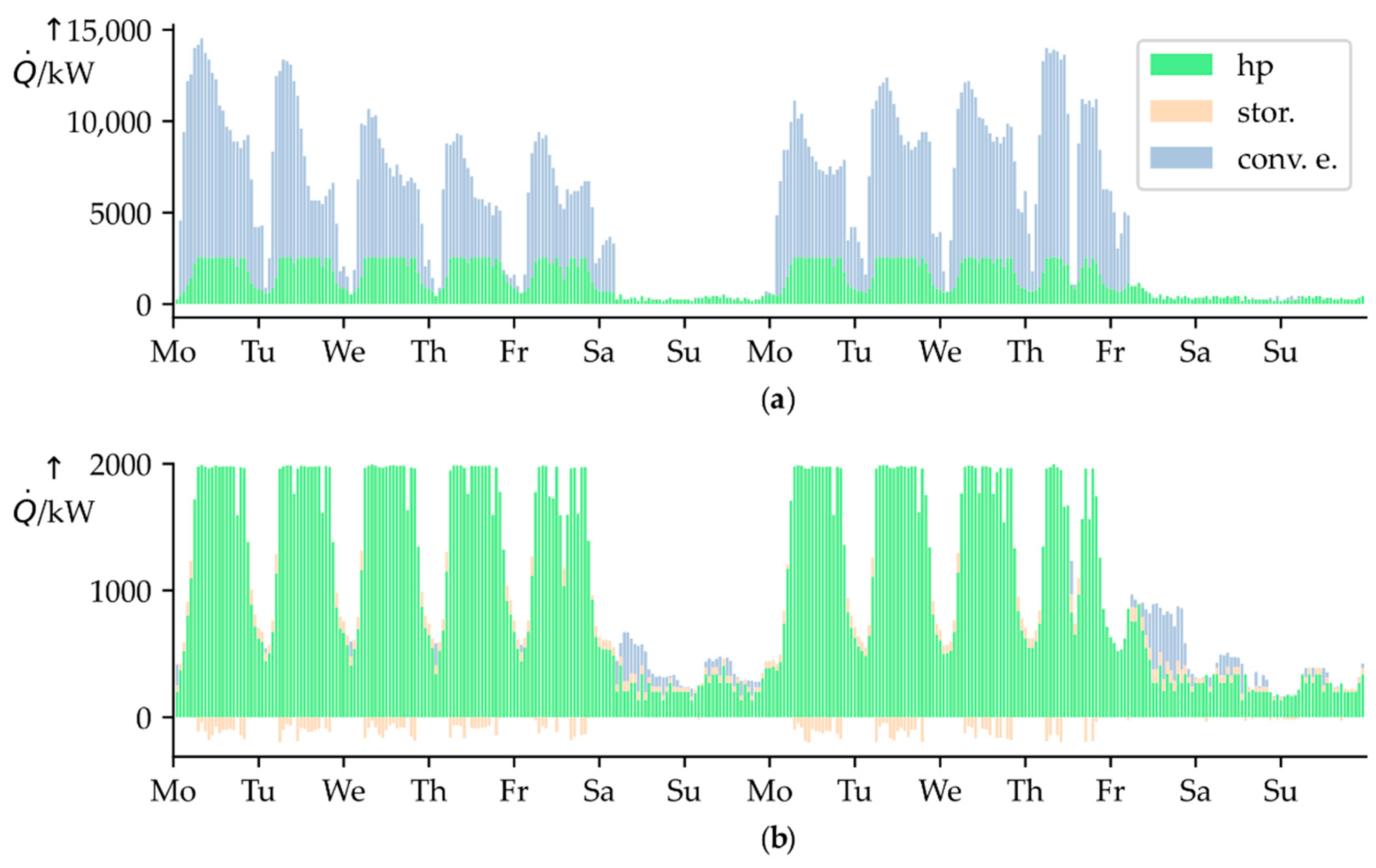
The storage is primarily unloaded during the weekend when the heating demand (see Figure 6) is not sufficiently high to run all heat pumps available. During the week, heat pump operation is limited only by cooling demand, as observable in Figure 6. Notably, the storage is more loaded than unloaded (11.9%), which results in unused energy over the year. Therefore, the storage size calculated by the model should be viewed critically.

In conclusion, the heat pump operation during the week is very stable, because of the flattened slope of the cooling demand (Figure 5). The coverage of demand in Figure 6 and the high NPV suggest that the tool attempts to completely cover cooling demand with heat pumps regardless of parameter variation. Exceptions might include variations of specific costs and temperatures.

3.2.2. Demand

For the parameter variation of demand, it is reduced from 80% to 60% to 40%. First, the heating demand is reduced, followed by the cooling demand, and then both demands. The mass flow rate is adjusted so that the temperatures in the thermohydraulic network remain constant. The preselection of heat pumps remains the same as for the standard run because the algorithm calculates its preselection with the averaged cooling demand and not the heating demand. Other thermodynamic parameters stay unchanged.

The reduction of the heating demand has almost no effect on the results because even a 40% heating demand allows complete coverage of the cooling demand by heat pump operation. In addition, the heat pump constellation stays the same for all three reduction steps (80%, 60%, 40%), as

Table 5. Results of the 80%, 60% and 40% heating demand run (own representation).

Heat Pump	$\mathit{C}\mathit{O}{\mathit{P}}_{\mathit{i}}^{\mathbf{av}}$	$\mathit{a}\mathit{m}$
BWC 351 A07	4.39	2
BW 351 A07	4.29	0
BW 351 A18	4.27	6
BW 301 A10	4.25	0
BW 301 A08	4.08	0

demonstrates. However, the tool decides to buy two small heat pumps instead of one large-scale heat pump, which can be justified by a greater need for flexibility in low-peak areas of the heating demand. This decision results in a lower NPV compared to the standard run.

The reduction of the cooling demand results in a much more significant change because the reduced demand limits heat pump operation. The tool decides to buy three small heat pumps (BWC 351 A07) and five large-scale heat pumps (BW 351 A18). Moreover, it selects cold water storage with a volume of 1528 L. The ratio of loading to unloading is 16.75%; the tool loads the storage without unloading it to cover more heating demand with the heat pumps. This raises the question of whether the cold water storage size for this application makes sense in practice. The NPV is reduced by almost 20% in comparison to the standard; this reduction of cooling demand by 20% has a greater impact than reducing heating demand by 60%.

A similar development as for the 80% cooling demand is observed with the 60% cooling demand. The NPV is drastically reduced, fewer heat pumps are purchased (four large-scale heat pumps—BW 351 A18, two small heat pumps—BWC 351 A07), and the cold water storage size is reduced to 835 L (loading/unloading ratio of 22.5%). Apparently, larger storage is no longer economical, and the energy surplus in the storage indicates that the choice of the cold water storage is again critical and should, if necessary, be lower in practice. Here, the NPV has been reduced by 38% compared with the standard. The cooling demand remains almost completely covered by heat pumps. The test run with a 40% cooling demand results in the purchase of three large-scale heat pumps (BW 351 A18) and cold water storage with a volume of 777 L, whose loading surplus is 21.6%. The NPV is reduced by 59% and develops in line with the other reduction steps of the cooling demand.

Within the joint stepwise reduction of the demand, a similar behavior as that of the reduction of the cooling demand is to be expected, since here, a clear dependence is presented. Therefore, the tool arrives at similar results, with the 80% heating and 80% cooling demand, as for the 80% cooling demand. The tool selects the same heat pump configuration as that of the 20% cooling demand reduction. The purchased cold water storage has a volume of 1940 L and a loading surplus of 15.5%. The excess in the storage is lower because the heating demand is reduced as well. The coverage of demand is analogous to the case of the 80% cooling demand. The NPV has been reduced by 21%, which differs slightly (<1%) from the case of the 80% cooling demand.

The cases for the reduction of the cooling and heating demand by 40% and 60% result in a similar configuration as with the cases for the cooling demand reduction by 40% and 60%. The NPV is 4% lower with the 40% reduction of heating and cooling demand and 6% lower with the 60% reduction of heating and cooling demand.

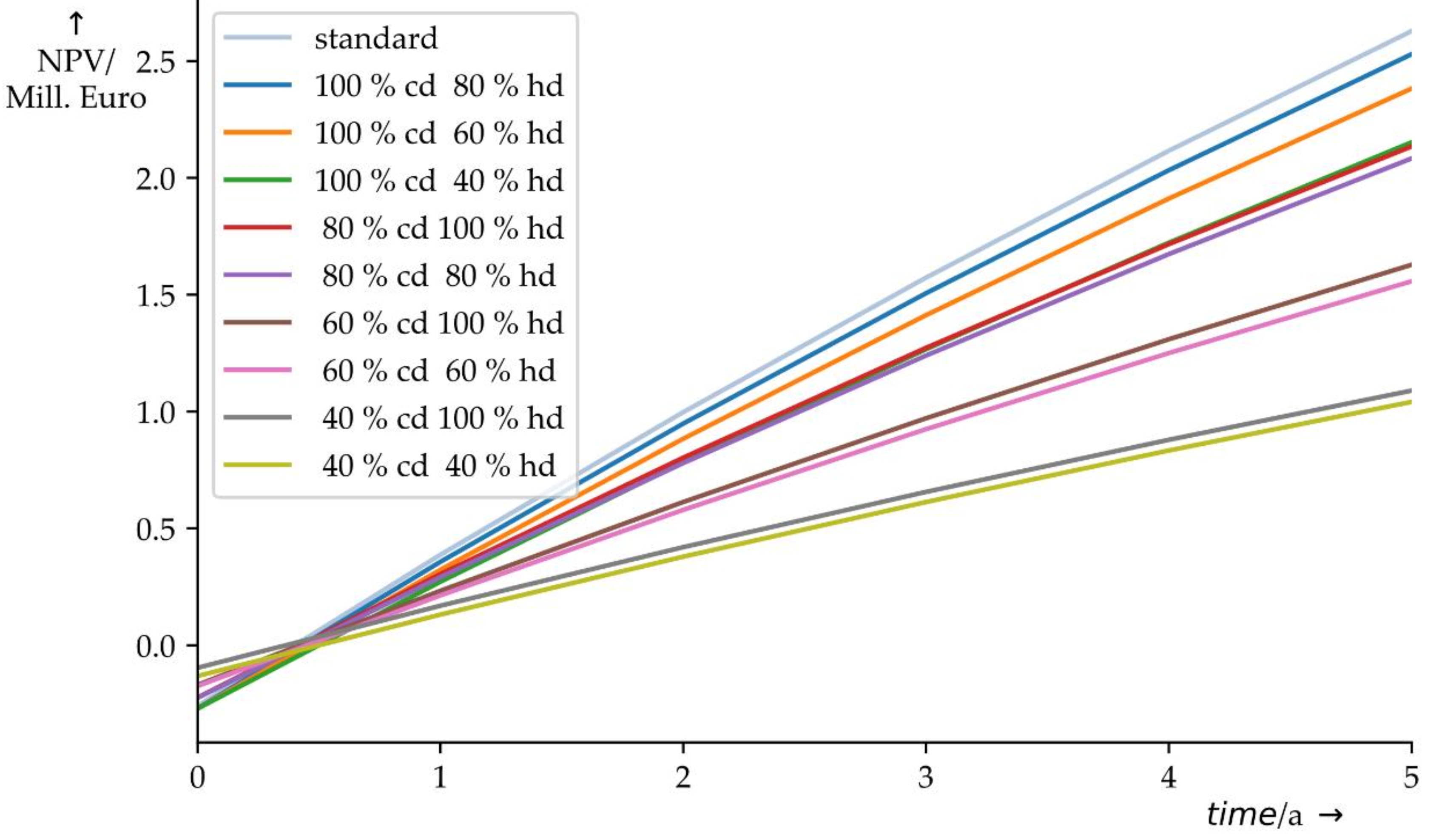
Figure 7 displays the NPV development of all changes in demand. In sum, the following insights can be gained from the change in demand:

• The tool will always try to completely cover the lower demand with heat pumps (in this example, this refers to the cooling demand).
• The chosen volume of storage might not make sense despite the tool’s selection, as it may be primarily loaded.
• The size of cold water storage depends on both the heating and cooling demand.
• The NPV is primarily dependent on the lower demand curve (in this example, this refers to the cooling demand).

3.2.3. Temperature

For the temperature variation, the flow temperatures are changed. The difference between the return and flow temperature remains a maximum of 6 K in both networks. Regardless of the temperatures, no changes are made to the specified standard. Furthermore, it is possible that the preselection changes, as other heat pumps in the temperature area, may have a better COP. The temperature change will have little effect on the coverage of demand; therefore, the focus lies on the development of the NPV.

Table A1. Results of $T_{\mathrm{flow},\mathrm{c}}$ = 5 °C and $T_{\mathrm{flow},\mathrm{w}}$ = 60 °C run with a 1945 L cold water storage and an NPV of 2.16 Mill. € (own representation).

Heat Pump	$\mathit{C}\mathit{O}{\mathit{P}}_{\mathit{i}}^{\mathbf{av}}$	$\mathit{a}\mathit{m}$
BWC 351 A07	3.44	6
BW 351 A07	3.38	0
BW 351 A18	3.44	8
BW 301 A10	2.89	0
BWC 201 A17	2.83	0

,

Table A2. Results of $T_{\mathrm{flow},\mathrm{c}}$ = 5 °C and $T_{\mathrm{flow},\mathrm{w}}$ = 66 °C run with a 1977 L cold water storage and an NPV of 1.8 Mill. € (own representation).

Heat Pump	$\mathit{C}\mathit{O}{\mathit{P}}_{\mathit{i}}^{\mathbf{av}}$	$\mathit{a}\mathit{m}$
BW 351 A18	3.02	8
BWC 351 A07	2.97	8
BW 351 A07	2.93	1
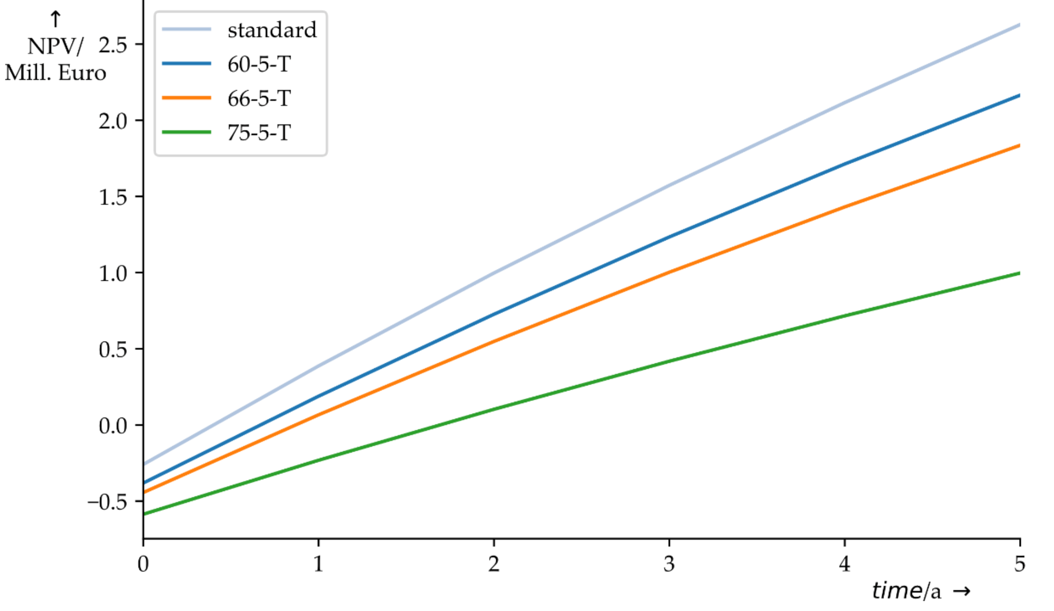
BWC 201 A17	2.19	0
BW 301 A10	2.18	0

and

Table A3. Results of $T_{\mathrm{flow},\mathrm{c}}$ = 5 °C and $T_{\mathrm{flow},\mathrm{w}}$ = 75 °C run with a 1097 L cold water storage and an NPV of 1 Mill. € (own representation).

Heat Pump	$\mathit{C}\mathit{O}{\mathit{P}}_{\mathit{i}}^{\mathbf{av}}$	$\mathit{a}\mathit{m}$
BW 351 A18	2.39	8
BWC 351 A07	2.26	8
BW 351 A07	2.25	8
BWC 201 A17	1.23	0
BWC 201 A10	1.13	0

reveal that the tool increases the number of heat pumps to fully cover the cooling demand with the heat pump operation. Due to the decrease in the COP caused by a higher temperature spread, more heat pumps are needed. Additionally, the NPV decreases with the temperature spread (see Figure 8) as expected because the starting investment increases and because the financial advantage of heat pump operation decreases with their COP. If the flow temperature of the heating circuit is equal to 90 °C and the flow temperature of the cooling circuit is equal to 5 °C, the purchase of a heat pump is no longer economical.

The temperature variation leads to the following conclusions:

• A rising temperature spread between the heat source and the heat sink leads to lower efficiency.
• As long as the purchase of a heat pump is economical, the cooling demand will be covered fully by heat pumps.
• With a flow temperature of the cooling circuit of 5 °C and a flow temperature of the heating circuit of 90 °C, the purchase of a heat pump is no longer economical.

3.2.4. Costs

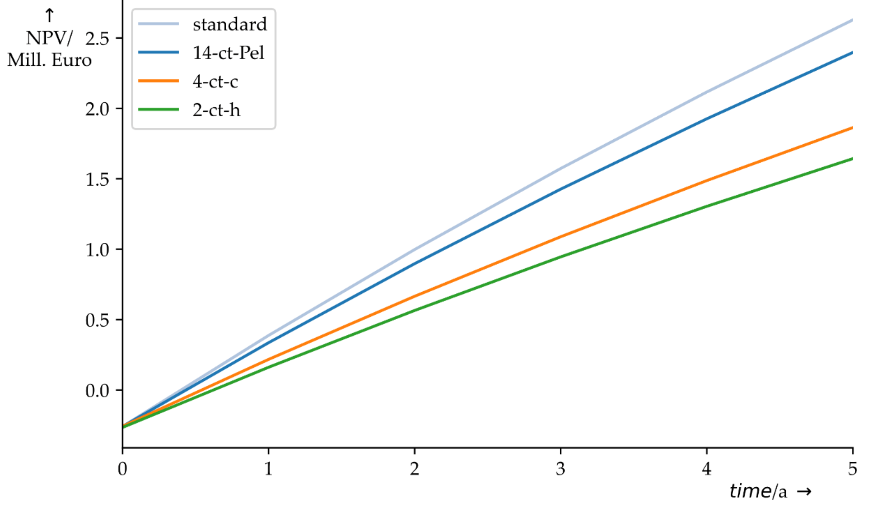
The variation of specific costs does not influence preselection or COP; therefore, the preselected heat pumps are the same as for the standard run (Table 4). Figure 9 displays the reduction of specific costs for heating and cooling by 2 ct·kWh⁻¹, and it can be observed that the reduction of specific heating costs results in a much gentler slope of the NPV function than the reduction of specific cooling costs. This slope difference can be justified by Equations (3) and (6). If a heat pump is running, it can provide more heating energy than cooling energy; therefore, less heat must be provided by the conventional energy converter. Additionally, it can be noted that the increase in specific costs for electricity has the lowest influence on the NPV because of the COP (see Equations (3) and (6)).

Even if the specific costs for heating and cooling are reduced to 2 ct·kWh⁻¹, it remains economical to purchase a heat pump. The high demand for the industrial use case allows for refinancing the heat pump to reach the break-even point after the payback period with an NPV of approximately 150,000 €. Only if either of the specific costs is reduced to 1 ct·kWh⁻¹, the tool will not decide to purchase a heat pump.

3.2.5. Storage

To further analyze the influence of storage integration, a model without the flexibility option is tested. For this run, the input parameters for the MILP model remain unchanged; therefore, the preselection and average of the COP remain the same.

The tool decides to buy another small heat pump (BWC 351 A07) on top of the heat pump configuration of the standard run. This decision can be justified by a lack of flexibility to cover the acyclic demand for heating and cooling, which results in a slightly lower NPV of 2.577 Mill. €. Therefore, the storage model has a reason to exist in the MILP model.

3.2.6. Preselection Algorithm

The altering of the preselection will test the algorithm and its influence on the optimization. To test the algorithm, the preselection allows all 15 heat pumps ($ms=15$), and the tool is allowed to purchase each heat pump three times ($am=3$). This high variety of heat pump models (standard run: $ms=5$) reveals whether any heat pumps are purchased that have not passed the preselection in the standard run. This faulty selection can occur primarily because the optimizer classifies the nominal heat flow rate as a more important criterion than the COP. However, if all heat pumps pass the nominal heat flow rate criterion (Equation (16)) then the preselection algorithm selects—for the standard run—the five models with the highest COP. These five models may have a much lower nominal heat flow rate than other models, but now the optimizer can only choose between the five models.

The tool decides to purchase three large-scale heat pumps of the same model (BWC 201 A17), which has not passed preselection in the standard run. The optimizer’s decision can be justified by the large nominal heat flow rate of 172 kW. This shows that the preselection negatively affects the outcome of the optimizer, as it reduces the variety of selection. However, without the preselection, the standard run with 15 min time steps computes over one week, while the preselection reduces the computational time to 14 h on a machine with an Intel(R) Core(TM) i7-7700K central processing unit of 4.20 GHz and random-access memory of 16 GB.

3.3. Analysis with the Simulation Model

The comparison of the simulation model and the optimization model checks the assumption that the heat pump implementation does not change the temperatures in the network, and therefore, the COP and the maximum electrical power of the heat pumps can be calculated prior to the optimization. Validation via the simulation model is performed using an optimization run with 15 min time steps to improve accuracy. The standard input parameters are used. The preselection is reduced to three heat pumps that can be purchased five times to reduce computational time. A large-scale heat pump (BW 351 A18) has been purchased five times, and seven small heat pumps (five times BWC 351 A07, twice BW 351 A07) have been purchased. In addition, cold water storage with a volume of 6100 L has been selected. The NPV of the optimization has a value of 2.5 Mill. € and the simulation calculates a value of 2.3 Mill. €, which results in an error of 7.68% (Equation (17)).

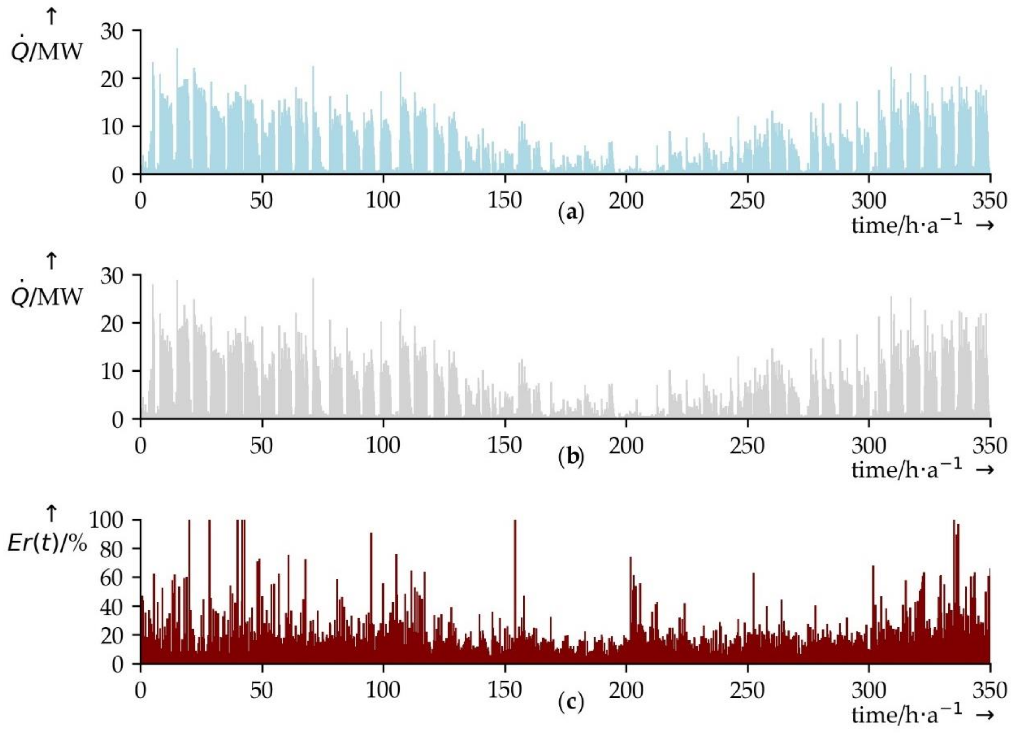
Figure 10 provides more information about the actual difference of heat pump operation between the simulation and the optimization than the error does. The heat flow rate of the conventional energy converter is displayed for the optimization (a) and the simulation (b). The difference between these rates (c) is also observed. If the simulated conventional energy converter requires more or less power to reach the flow temperature than the optimized conventional energy converter, it will indicate a failure of the assumption concerning the temperatures in the network. This failure would result in a false optimization since the COP is calculated prior to the MILP run. However, both conventional energy converters behave similarly. The analysis with the aid of the simulation model provides valuable knowledge regarding the application area of the tool. The assumption for the temperatures appears to be especially critical for peak areas greater than 7 MW (heating demand). This development in peak areas leads to the conclusion that an application of the tool is favorable for demands where high base loads of heating and cooling must be covered.

4. Discussion and Conclusions

This paper presents a method to calculate the optimal integration of heat pumps into industrial thermohydraulic networks by considering design decisions and operation strategies. The method consists of a heat pump database, a preselection algorithm, a mathematical model, and a simulation model. The mathematical model, as a MILP representation, can model heat pump integration combining design and optimal control with consideration of partial load behavior and simultaneous provision of heating and cooling. Additionally, the integration of storages for heating and cooling is displayed.

The parameter analysis has considered, for example, varying energy demands, temperatures, and costs, showing that the mathematical model behaves correctly within its framework and that the results of the analysis are logically valid. Moreover, the results of the calculations show that the integration of heat pumps in combination with energy storage is highly energy-efficient which positively affects the opex, as shown in the high NPVs. However, the chosen industrial example is seemingly ideal for heat pump utilization based on the developed application tool, as cooling demand can be covered by heat pumps alone. This good fit explains the extremely high profits achieved in the test runs. To tackle the relatively high calculation times of the mathematical model, a preselection algorithm has been implemented. On the one hand, this may lead to a less-than-optimal configuration of heat pumps and storages; on the other hand, the reduced calculation time makes the tool applicable. A first parameter study indicates that the preselection algorithm decides properly which technologies should be included in the optimization run.

The integrated simulation model primarily verifies assumptions about temperature development and, thus, allows for new modeling of heat pumps by calculating the COP in the baseload range beforehand. This assumption is correct in most cases, especially in baseload scenarios in which heat pumps can be used efficiently. Nevertheless, the simulation model shows a relatively high error in peak load scenarios, in the use case in ranges higher than 7 MW. The overall error between the mathematical and the simulation model is 7.7% within the use case. Nevertheless, the tool offers optimum control of heat pumps, conventional energy converters, and storages, giving it a decisive advantage over conventional designs.

In conclusion, the parameter analysis shows three major important outcomes. Firstly, the tool reacts sensibly to the variation of cooling demand because it limits heat pump operation. Therefore, a clear dependence of the NPV on the lower demand curve is shown. Secondly, the effect of the temperature spread between the heating and cooling network also has a major impact on the NPV because a high temperature spread results in a lower COP. Lastly, the specific costs obviously affect the outcome of the objective function. However, the specific cost for electricity has a much lower impact on the NPV than do costs for heating and cooling (see Figure 9). This differential impact occurs because the generated heating and cooling energy is larger than the necessary electrical input for the heat pump if the COP is over 1 (see Equations (3) and (6)). This clearly emphasizes the importance of heat pumps in the industry and especially the parallel provision of heating and cooling by heat pump operation. Additionally, the model provides users with a heat pump library to select from, which can be customized for their purposes instead of assuming a static heat pump integration [12,13,14,15]. Another asset of the model is the storage integration because the significant difference in the demand curves cannot efficiently be covered by heat pump operation, as shown in Section 3.2.5.

Overall, the presented method can provide the optimum design of heat pumps and storages, based on the control strategy for 15 min time steps over one year depending on historical data from the thermohydraulic network. The comparison of the NPV from the MILP model ($C^{\mathrm{tot},\mathrm{opti}}$) and the simulation model ($C^{\mathrm{tot},\mathrm{sim}}$) reveals an accuracy of the optimization model of more than 90% (see Equation (17)). As the model does not consider all costs of a planning and implementation process (planning costs, costs for pipes and construction, etc.), in future works, these costs should be analyzed and integrated into the tool. The method shows that the planning process should involve a detailed simulation model to verify the thermohydraulic design of the optimization output. In addition to the design, the simulation can react to the optimized operation to further improve the control of generators. Lastly, a more detailed storage model in the simulation would positively impact the decision-making certainty of a planner. A graphical user interface would increase the usability of the planning tool.

References

- Ittershagen, M. Erneuerbare Energien in Zahlen. Available online: https://www.umweltbundesamt.de/themen/klima-energie/erneuerbare-energien/erneuerbare-energien-in-zahlen#uberblick (accessed on 1 July 2020).
- Hüttmann, M. CO2-Freie Wärme für Industrie und Gewerbe mit Solarthermie. Available online: https://www.dgs.de/news/en-detail/211218-co2-freie-waerme-fuer-industrie-und-gewerbe-mit-solarthermie/ (accessed on 7 September 2020).
- Deutscher Bundestag. Klimaschutzprogramm 2030 der Bundesregierung zur Umsetzung des Klimaschutzplans 2050. Available online: https://www.bundesregierung.de/resource/blob/975226/1679914/e01d6bd855f09bf05cf7498e06d0a3ff/2019-10-09-klima-massnahmen-data.pdf?download=1 (accessed on 1 July 2020).
- Wolf, S.; Fahl, U.; Blesl, M.; Voß, A.; Jakobs, R. Analyse des Potenzials von Industriewärmepumpen in Deutschland; Final Report to Federal Ministry for Economic Affairs and Energy (BMWi) and Energy Baden-Wuerttemberg AG (EnBW); Institute for Energy Economics and Rational Energy Use (IER) and Information Center for Heat Pumps and Refrigeration Technology (IZW): Stuttgart, Germany, 2014. [Google Scholar]
- Nowak, T. Heat Pumps. In Integrating Technologies to Decarbonise Heating and Cooling; Technical Report of European Copper Institute: Brussels, Belgium, 2018. [Google Scholar]
- Verein Deutscher Ingenieure. Hydraulik in Anlagen der Technischen Gebäudeausrüstung Hydraulische Schaltungen, 23.100.01, 91.140.10 (VDI 2073). Available online: https://www.vdi.de/richtlinien/details/vdi-2073-blatt-2-hydraulik-in-anlagen-der-technischen-gebaeudeausruestung-hydraulischer-abgleich-1 (accessed on 8 October 2019).
- Viessmann. Planungsanleitung. Sole/Wasser- und Wasser/Wasser-Wärmepumpenein- und Zweistufig, 5,8 bis 117,8 kW. Available online: https://www.manualslib.de/manual/441762/Viessmann-Vitocal-300-G-Typ-Bw-301-A.html#manual (accessed on 11 August 2020).
- Heinrich, C.; Wittig, S.; Albring, P.; Richter, L.; Safarik, M.; Böhm, U.; Hantsch, A. Nachhaltige Kälteversorgung in Deutschland an den Beispielen Gebäudeklimatisierung und Industrie. Clim. Chang. 2014, 25, 82–83. [Google Scholar]
- Frisch, S.; Pehnt, M.; Otter, P.; Nast, M. Prozesswärme im Marktanreizprogramm. In Zwischenbericht zu Perspektivische Weiterentwicklung des Marktanreizprogramms FKZ 03MAP123; Interim Report to Federal Ministry for Economic Affairs and Energy (BMWi); Institute for Energy and Environmental Research (ifeu): Heidelberg, Germany; German Aerospace Center (DLR): Stuttgart, Germany, 2010. [Google Scholar]
- Vardakas, J.S.; Zorba, N.; Verikoukis, C.V. A Survey on Demand Response Programs in Smart Grids: Pricing Methods and Optimization Algorithms. IEEE Commun. Surv. Tutor. 2014, 17, 152–178. [Google Scholar] [CrossRef]
- Hart, W.E. Pyomo-Optimization Modeling in Python, 2nd ed.; Springer: Cham, Switzerland, 2017; ISBN 978-3-319-58819-3. [Google Scholar]
- Schütz, T.; Harb, H.; Streblow, R.; Mueller, D. Comparison of models for thermal energy storage units and heat pumps in mixed integer linear programming. In Proceedings of the 28th International Conference on Efficiency, Cost, Optimization, Simulation and Environmental Impact of Energy Systems (ECOS), Pau, France, 29 June 2015. [Google Scholar]
- Fang, C.; Xu, Q.; Wang, S.; Ruan, Y. Operation optimization of heat pump in compound heating system. Energy Procedia 2018, 152, 45–50. [Google Scholar] [CrossRef]
- Schlosser, F.; Seevers, J.-P.; Peesel, R.-H. System efficient integration of standby control and heat pump storage systems in manufacturing processes. Energy 2019, 181, 395–406. [Google Scholar] [CrossRef]
- Kanga, Z.; Zhoua, X.; Zhaoa, Y.; Wanga, R.; Wang, X. Study on Optimization of Underground Water Source Heat Pump. Procedia Eng. 2017, 205, 1691–1697. [Google Scholar] [CrossRef]
- Held, E. Wie funktioniert eigentlich eine Wärmepumpe? Gezügelte Leistung. SBZ Monteur 2017, 21, 10–15. [Google Scholar]
- Oppelt, T. Modell zur Auslegung und Betriebsoptimierung von Nah- und Fernkältenetzen. Ph.D. Thesis, Technical University of Chemnitz, Chemnitz, Germany, 2015. Available online: https://monarch.qucosa.de/api/qucosa%3A20314/attachment/ATT-0/ (accessed on 30 October 2020).
- Malherbe, A. DYMOLA Systems Engineering. Available online: https://www.3ds.com/de/produkte-und-services/catia/produkte/dymola/ (accessed on 15 July 2020).
- Functional Mock-Up Interface. Available online: https://fmi-standard.org/ (accessed on 15 July 2020).
- Konstantin, P. Praxisbuch Energiewirtschaft: Energieumwandlung, Transport und Beschaffung, Übertragungsnetzausbau und Kernenergieausstieg, 4th ed.; Springer: Berlin/Heidelberg, Germany, 2017; p. 14. ISBN 978-3-662-49822-4. [Google Scholar]
- Chiasson, A. Geothermal heat pump and heat engine systems. In Theory and Practice; Wiley: Hoboken, NJ, USA, 2016; pp. 312–314, 327–328. ISBN 9781118961971. [Google Scholar]
- Weisberg, S. Applied Linear Regression, 4th ed.; Wiley: Hoboken, NJ, USA, 2014; pp. 51–53. ISBN 9781118386088. [Google Scholar]
- Müller, C. Leistungszahlen für Kälte-, Klima- und Wärmepumpensysteme. Friscaldo 2008, 1, 31–33. [Google Scholar]
- Hülsken, C. Erneuerbare energie für die industrie: Prozesswärme aus bioenergie sorgt für unabhängigkeit und klimaschutz. Renews Kompakt 2017, 38, 1–5. [Google Scholar]
- Modelica Association. Modelica Libraries. Available online: https://www.modelica.org/libraries (accessed on 8 October 2020).
- Grave, K.; Hazrat, M.; Boeve, S.; Blücher, F.V.; Bourgault, C.; Bader, N.; Breitschopf, B.; Friedrichsen, N.; Arens, M.; Aydemir, A.; et al. Stromkosten der energieintensiven Industrie. In Ein Internationaler Vergleich; Technical Report to Federal Ministry for Economic Affairs and Energy (BMWi); Fraunhofer ISI and ECOFYS Germany GmbH: Berlin, Germany, 2015. [Google Scholar]
- Illner, B.; Bünting, F. Industrie 4.0: Finanzierung von Investitionen. Available online: https://www.vdma.org/documents/105628/878344/Investitionen+in+Industrie+40.pdf/abafbde7-51d8-4281-af3e-f567361ef979 (accessed on 9 October 2019).
- Stiebel Eltron. OPERATION AND INSTALLATION: DHW Heat Pump. Available online: https://www.stiebel-eltron.com.au/download/1540529916_STIEBEL_ELTRON_Operation_and_Installation_WWK.pdf (accessed on 16 September 2020).
- Viessmann. Preisliste 2018 DE Heizsysteme. Available online: https://www.meinhausshop.de/media/pdf/meinhausshop-Viessmann-Hetzsysteme-Teil%201.PDF (accessed on 17 October 2019).
- Pang, X.-F. Water. In Molecular Structure and Properties; World Scientific Publishing Company: Singapore, 2014; pp. 92, 97. ISBN 9789814440431. [Google Scholar]
Figure 1.
Process heating and cooling in Germany depending on the industry, temperature range, and energy with the percentage of total process heating and cooling demand [8] (pp. 82–83) [9] (p. 6).
Figure 2.
Method for the planning tool with the MILP model as backbone.
Figure 3.
Concept of the model for a thermohydraulic network (heating or cooling) with the following four components: (a) consumer, (b) storage, (c) heat pump, and (d) conventional energy converter. The heat pump (c) has a connection to the second thermohydraulic network. The storage loading process is represented by a red arrow and the unloading process by a blue arrow [6] (p. 22).
Figure 4.
Simulation model in Dymola with the generation units (a) (heat pump and conventional energy converter), the storage (b), the distribution circuit (c), and a boundary (d).
Figure 5.
Annual duration line for cooling demand (a) and heating demand (b) (sensitive data from a company).
Figure 6.
Cumulative coverage of the heating demand (a) and cooling demand (b) for the standard in kW with heat pumps (green), storage (yellow), and conventional energy converter (blue) (own representation).
Figure 7.
NPV development over time for standard with the percentage reduction (80%, 60%, 40%) of heating demand, cooling demand, and both demands (own representation).
Figure 8.
NPV development over time for standard, = 5 °C and = 60 °C (60-5-T), = 5 °C and = 66 °C (66-5-T), = 5 °C and = 75 °C (75-5-T) (own representation).
Figure 9.
NPV development over time for standard, specific heating costs of 2 ct·kWh−1 (2-ct-h), specific cooling costs of 4 ct·kWh−1 (4-ct-c), and specific electric costs of 14 ct·kWh−1 (14-ct-Pel) (own representation).
Figure 10.
Heat flow rate of the optimized conventional energy converter (a), of the simulated conventional energy converter (b) and the error (c) between both heat flow rates (own representation).